Primer on Axion Physics

Abstract

I review the canonical axion potential, with an emphasis on the field theory underlying radial and angular modes of complex scalar fields. I present the explicit calculation of the instanton-induced breaking of the Goldstone field direction necessary to derive the canonical axion mass and decay constant relation. The primer is intended to serve an audience with elementary quantum field theory expertise.

I Introduction

Axions are hypothesized particles originally proposed to resolve the strong CP problem of the Standard Model. The essential mechanism of the axion solution is that the quantum chromodynamics (QCD) instanton-generated potential for the axion is minimized when the vacuum expectation value of the axion exactly cancels the (unknown) original $\bar{\Theta}$ parameter, leaving an effective $\bar{\Theta}_{\text{eff}}$ parameter that is vanishing. In this review, we will see the fundamental distinction between the axion potential and other, more common scalar potentials usually considered in quantum field theories, such as the Higgs potential of the Standard Model. We will also analyze the field theory from the modern viewpoint of Peccei-Quinn (PQ) symmetry, again making a distinction between the role of PQ symmetries relevant for axion physics and the more traditional electroweak gauge symmetry emphasized in Higgs physics. The goals of this primer are to derive and motivate the axion potential as a characteristic and benchmark model of pseudo-Nambu-Goldstone boson (pNGB) Lagrangians as well as to develop the basic phenomenological signals of axion and axion-like particles as ultralight dark matter candidates. Several excellent reviews of axion physics include Kim:2008hd ; Kawasaki:2013ae ; Graham:2015ouw ; Irastorza:2018dyq ; Hook:2018dlk ; DiLuzio:2020wdo ; Reece:2023czb , as well as the ever-evolving Particle Data Group review ParticleDataGroup:2022pth , which expertly cover the breadth of axion physics in cosmology, particle physics, and field theory at a high level. In contrast, this primer is designed to build axion physics from the ground up, assuming only a beginning level of quantum field theory knowledge.

The mathematical framework for fundamental laws of Nature, in particular the Standard Model, is quantum field theory, which is based on the quantum action $S=\int d^{4}x\mathcal{L}$, where the Lagrangian $\mathcal{L}$ (technically, the Lagrangian density, but we always call it the Lagrangian) is required to respect Poincaré invariance. Poincaré symmetry is Lorentz symmetry $\oplus$ translation symmetry, and is required to establish the familiar energy-momentum conservation laws as well as the characterization of particles according to half-integer representations for spin-angular momentum. This motivates starting with the simplest quantum field theory, namely that of a scalar field whose excitations are scalar particles with spin $0$.

II Scalar field theory

We begin with the field theory of a single scalar field $\phi$. Scalar fields assign a pure real number to every spacetime point, and thus they take the spacetime coordinate as their argument. For a scalar field with mass $m$ and no interactions, we can write the Lagrangian (density) as

$$\mathcal{L}=\frac{1}{2}\left(\partial_{\mu}\phi\right)^{2}-\frac{1}{2}m^{2}\phi^{2}\ .$$ (1)

Analyzing the Euler-Lagrange equation of motion dictated by this Lagrangian will recover the familiar Klein-Gordon equation governing free scalars with a mass $m$, assuming $m>0$.

If there is a second scalar field with exactly the same mass, then the two fields can be combined into a single complex scalar field $\Phi$, where the real part of $\Phi$ is the number assigned by the original $\phi$ field and the imaginary part of $\Phi$ represents the second scalar field. Clearly, the Lagrangian in this case can be written as

$$\mathcal{L}=\left|\partial_{\mu}\Phi\right|^{2}-m^{2}|\Phi|^{2}\ .$$ (2)

Note the prefactors of the kinetic and mass term are twice as large as the real scalar Lagrangian, reflecting the existence of two distinct real degrees of freedom.

To connect to Higgs physics and the phenomenon of spontaneous symmetry breaking, we can now add a quartic interaction. We have

$$\mathcal{L}=\left|\partial_{\mu}\Phi\right|^{2}-m^{2}|\Phi|^{2}\ -\lambda|\Phi|^{4}\ .$$ (3)

We remark that the Lagrangian is always the kinetic energy minus potential energy, and so we can analyze the potential

$$V=m^{2}|\Phi|^{2}+\lambda|\Phi|^{4}\ .$$ (4)

In order for the potential to be bounded from below, we require $\lambda>0$, but we now have two possibilities for the sign of $m^{2}$. If $m^{2}>0$, the origin in field space is stable and the field has no vacuum expectation value (vev). If $m^{2}<0$, the origin in field space is unstable and the equation of motion for the scalar is extremized by a nonzero vev, $|\Phi|^{2}=v^{2}=-m^{2}/\lambda$. In either case, as we go to large excursions in field space, the potential energy grows because of $\lambda>0$, but the behavior near the origin in field space will distinguish the two potentials. As an aside, if we coupled the complex scalar field to a $U(1)$ gauge symmetry, replacing $\partial_{\mu}$ by a covariant derivative $D_{\mu}$ in the equation above, then the above Lagrangian would be the scalar part of the Abelian Higgs model, and the vev of the Higgs field would give a mass for the $U(1)$ gauge boson.

Importantly, the vacuum state of the theory is controlled by one constraint equation, $|\Phi|^{2}=v^{2}$, and therefore we have one degree of freedom that is unconstrained by the vacuum requirement. This is most evident when we change from a “Cartesian” field space parametrization to a “polar” parametrization,

$$\Phi=\left(\frac{v+h}{\sqrt{2}}\right)\exp(ia/v)\ ,$$ (5)

where $h$ and $a$ are the radial and angular modes of the complex field $\Phi$. When we write the original Lagrangian with this parametrization, we get

$$\mathcal{L}=\frac{1}{2}\left(\partial_{\mu}h\right)^{2}+\frac{1}{2}\left(\partial_{\mu}a\right)^{2}+\frac{1}{4}\lambda v^{4}-\lambda v^{2}h^{2}-\lambda vh^{3}-\frac{1}{4}\lambda h^{4}\ ,$$ (6)

where we notice that the angular field $a$ does not appear in the potential anymore while the radial field $h$ has a mass term $m_{h}=\sqrt{2\lambda}v$ as well as cubic and quartic self-interactions. We also remark the appearance of a constant energy (density) term in the potential, which plays no role in the dynamics at hand but would be relevant for the cosmological constant problem. The key point is that the angular field is a completely free and massless (pseduo)scalar field, and its (currently vanishing) dynamics are independent of the dynamics of the radial mode.

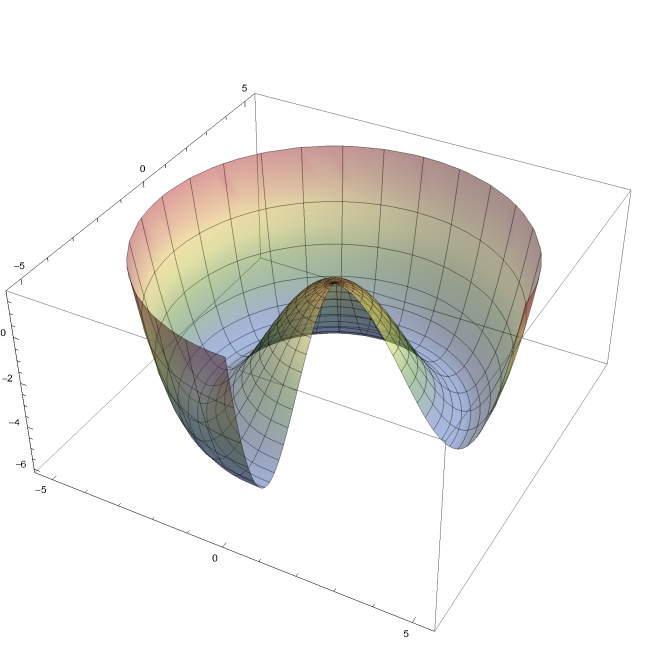
Figure 1: Schematic of the typical Higgs potential from a negative mass-squared term and a positive quartic term. The rotational symmetry is manifest for every point in field space and represents the Goldstone field direction.

We remark that the pseudoscalar nature of the $a$ field in Eq. (6) is only meaningful in the context of the embedding as the angular mode of the original complex scalar field $\Phi$. In particular, comparing Eq. (1) and the $a$-dependent term in Eq. (6) shows that Eq. (1) reduces to the $a$-dependent kinetic term if we neglect the mass $m$ in Eq. (1) and relabel $\phi$ to $a$. While this relabeling seems entirely safe given that the Lagrangians now coincide, we have to recall that $a$ is defined as a compact field direction via Eq. (5) while the original free scalar field $\phi$ lies on a noncompact field space. Formally, this distinction about compactness is reflected in the fact that the action $S$ has an extra periodic redundancy for $a\to a+2\pi v$ but not for a massless $\phi$, as evident from the polar decomposition in Eq. (5).

Importantly, the “zero point” in field space for $a$ is entirely degenerate and lies along the entirety of the circle in Fig. 1, as a result of the vev only being defined by its square. This is self-consistent with the Goldstone nature of $a$ having a continuous shift symmetry in Eq. (6), where any finite shift of $a$ leaves the Lagrangian invariant. In fact, the absence of an origin in field space is crucial for the axion solution to the strong CP problem, since it allows the axion to render any arbitrary $\bar{\Theta}$ starting value to (effectively) zero via the PQ mechanism.

III Instantons in Yang-Mills theory and the $\Theta$ vacuum energy

In this section, we review the non-perturbative calculation of the instanton-induced vacuum energy of Yang-Mills theory. This calculation is taken from the tour-de-force publicaation of ’t Hooft tHooft:1976snw and related literature on instantons Callan:1976je ; Callan:1977gz .

At the close of the last section, we demonstrated that the angular mode in a Higgsed potential is a free field with only a kinetic term. In more formal terms, the angular mode is a pseudoscalar field that has a continuous shift symmetry, meaning that any shift in the field has no effect on the Lagrangian. In particular, the field has no mass terms and no interactions, since masses and interactions violate the continuous shift symmetry. We remark that the generic nature of Goldstone bosons arising in ultraviolet extensions of the Standard Model can typically be mapped to the field theory at hand, although the key requirements to satisfy are that the ultraviolet fields exhibit Goldstones traversing a compact field space and the ultraviolet continuous symmetries are not gauged. This will be relevant for the extension of the axion parameter space to axion-like particles.

The continuous shift symmetry of the angular mode is explicitly broken if the symmetry has an anomaly. Anomalies are, by definition, quantum origins of symmetry breaking, and in the context of the axion, originate from the fact that the continuous shift symmetry for the pseudoscalar field is broken to a periodic shift symmetry from its axial coupling to fermions carrying color charges. The fact that the continuous shift symmetry has a nonzero anomaly with respect to the SM color gauge group is the defining property of Peccei-Quinn symmetries, and this $U(1)_{\text{PQ}}\times SU(3)_{c}^{2}$ anomaly explicitly breaks $U(1)_{\text{PQ}}$ to a periodic shift symmetry and reflected in the coupling of the axion field to the dual field strength tensor of QCD. At low energies, the dual field strength tensor of QCD leads to an instanton-induced potential for the axion, which we will derive in this section. We remark that the periodicity condition Eq. (5) and the color anomaly quantizes the vacuum structure of the axion field space according to a topological winding number, permitting domain wall solutions of the $a$ field interpolating between energetically degenerate but topologically distinct vacuum states.

III.1 Yang-Mills theory and Instantons

Instantons are a feature of Yang-Mills theories. The Yang-Mills action for an $SU(N)$ gauge theory in Minkowski metric is

$$\mathcal{L}=-\frac{1}{4}G_{\mu\nu}^{a}G^{\mu\nu,a},$$ (7)

where $G_{\mu\nu}^{a}\equiv\partial_{\mu}A_{\nu}^{a}-\partial_{\nu}A_{\mu}^{a}+g_{s}f^{abc}A_{\mu}^{b}A_{\nu}^{c}$. The simplest method for deriving the instanton solution follows Belavin, Polyakov, Schwartz, and Tyupkin (BPST) Belavin:1975fg .

First, we define $\tilde{G}^{a}=\frac{1}{2}\epsilon_{\mu\nu\rho\sigma}G^{a}_{\rho\sigma}$ for the totally antisymmetric tensor $\epsilon_{\mu\nu\rho\sigma}$ and $\epsilon_{0123}=1$. Then, since $G\tilde{G}$ is a total derivative, and since we are looking for classical field solutions to the action with minimized action, a unit instanton satisfies the quantization constraint

$$\int d^{4}x_{E}\frac{g_{s}^{2}}{32\pi^{2}}G\tilde{G}=\int d^{4}x_{E}\frac{g_{s}^{2}}{64\pi^{2}}\epsilon^{\mu\nu\rho\sigma}G_{\mu\nu}^{a}G_{\rho\sigma}^{a}=1\ ,$$ (8)

where $x_{E}$ is the Euclidean spacetime coordinate. We will relate this quantization constraint to the Chern-Simons topological current shortly.

The procedure from BPST is to consider the minimal action of the gauge fields arising from the inequality

$$0 \leq\int d^{4}x_{E}\left(G_{\mu\nu}^{a}\pm\frac{1}{2}\epsilon_{\mu\nu\rho\sigma}G_{\rho\sigma}^{a}\right)^{2}$$

$$=\int d^{4}x_{E}\left(G_{\mu\nu}^{a}\pm\epsilon_{\mu\nu\rho\sigma}G_{\mu\nu}^{a}G_{\rho\sigma}^{a}+\frac{1}{4}\epsilon_{\mu\nu\rho\sigma}\epsilon_{\mu\nu\eta\theta}G_{\rho\sigma}^{a}G_{\eta\theta}^{a}\right)$$

$$=\int d^{4}x_{E}\left[2(G_{\mu\nu})^{2}\pm 2\left(\frac{1}{2}\epsilon_{\mu\nu\rho\sigma}G_{\mu\nu}^{a}G_{\rho\sigma}^{a}\right)\right]\ .$$ (9)

In order to saturate the extremization condition, we must solve the first-order differential equation

$$G_{\mu\nu}^{a}=\pm\frac{1}{2}\epsilon_{\mu\nu\rho\sigma}G_{\rho\sigma}^{a}\ ,$$ (10)

for $A_{\mu}$ field solutions, where $+$ denotes self-dual fields and $-$ indicates anti-self-dual fields. The explicit profile of the instanton solution is essentially a monopole in group space, and can be written using ’t Hooft symbols tHooft:1976snw ; Shifman:2022shi . For example, an $SU(2)$ instanton can be written in temporal gauge ( $A_{0}(\vec{x})=0$ ) as the gauge field

$$A_{i}(\vec{x})=iU_{1}(\vec{x})\partial_{i}U_{1}^{\dagger}(\vec{x}),$$ (11)

where the $i=1,2,3$ subscripts refer to $\hat{x}$, $\hat{y}$, and $\hat{z}$ components of the vector field and $U_{1}(\vec{x})$ is the $SU(2)$-valued group matrix

$$U_{1}(\vec{x})=\exp\left(i\pi\vec{x}\cdot\vec{\tau}/\sqrt{|\vec{x}|^{2}+\rho^{2}}\right),$$ (12)

where $\vec{\tau}=\vec{\sigma}/2$ are the $SU(2)$ generators and $\rho$ is a parameter characterizing the instanton size. This prescription generalizes to higher winding numbers by replacing $U_{1}$ by $U_{n}\equiv U_{1}^{n}$ for the desired winding number $n$. An additional complication arises when considering instanton solutions for groups larger than $SU(2)$, but a fortunate simplification arises from the fact that all $SU(N)$ groups share the same homotopy classifcation $\Pi_{3}(SU(N))=\mathbb{Z}$, which essentially means that all instanton solutions of a given winding number in an $SU(N)$ group are smoothly deformable into each other. Thus, it is sufficient to characterize instanton solutions in an arbitrary $SU(N)$ group by first considering a convenient $SU(2)$ subgroup and then augmenting the solutions by an appropriate “index of embedding” that keeps track of the dimensionality of the larger group space Shifman:2022shi ; Csaki:1998vv .

We remark that a standard introduction to instantons motivates Eq. (11) as gauge-equivalent to $0$. From this perspective, we note that (still in temporal gauge) trivial $A_{i}=0$ solutions to the field equations obviously minimize the Yang-Mills action. Yet since the action is defined by an integral over (Euclidean) spacetime, we should simultaneously consider all gauge field configurations that are equivalent to the trivial $A_{i}=0$ solution, which motivates us to consider “pure gauge” field configurations for $A_{i}$ as written in Eq. (11). Imposing the (anti-)self-duality condition from Eq. (10) then leads to the BPST (anti-)instanton solution.

III.2 The $\Theta$-vacuum in Yang-Mills

The main consequence of instanton solutions in Yang-Mills theory is its impact on the vacuum structure. We first illustrate this point by noting the unit instanton solution satisfying Eq. (8) corresponds to the flow of the Chern-Simons current Shifman:2022shi

$$K^{\mu}=2\epsilon^{\mu\nu\alpha\beta}\left(A_{\nu}^{a}\partial_{\alpha}A_{\beta}^{a}+\frac{g}{3}f^{abc}A_{\nu}^{a}A_{\alpha}^{b}A_{\beta}^{c}\right)\ ,$$ (13)

where the charge of the $K^{\mu}$ current is the usual integral of $K^{0}$ over three-dimensional space,

$$\mathcal{K}=\frac{g^{2}}{32\pi^{2}}\int d^{3}xK^{0}(x)\ .$$ (14)

While the Chern-Simons current is not gauge-invariant and hence not a physical current, its divergence is gauge-invariant and actually the familiar $G\tilde{G}$ operator,

$$\partial_{\mu}K^{\mu}=G\tilde{G},$$ (15)

which allows us to identify the unit instanton as carrying Chern-Simons topological charge. Consequently, the vacuum state of Yang-Mills theory is an infinitely degenerate vacuum state with “pre-vacua” labeled by Chern-Simons charge, as required from the homotopy classification.

We now calculate the vacuum energy of $SU(2)$ Yang-Mills theory, which can be obtained using the functional integral method. We start with

$$\exp\ ({-\mathcal{E}~{}V\cdot T}) =\int\mathcal{D}A\exp(-S_{E}\left[A\right])\ ,$$ (16)

where $S_{E}[A]$ is the Euclidean action corresponding to Eq. (7) and $\mathcal{E}$ is the vacuum energy density and $V\cdot T$ is the volume of Euclidean spacetime. The functional integral is a sum over topological sectors with winding numbers $w$ as

$$\exp\ ({-\mathcal{E}~{}V\cdot T}) =1\times\int\left[\mathcal{D}A\right]_{w=0}\exp\left[-\int\frac{1}{2}\delta A\cdot(-\partial^{2})\delta A\right]$$

$$+\exp(-8\pi^{2}/g^{2})\times 2\int\left[\mathcal{D}A\right]_{w=\pm 1}\exp\left[-\int\frac{1}{2}\delta A\cdot(-\partial^{2})\delta A\right]$$

$$+\ldots\ ,$$ (17)

where the $\ldots$ indicate a sum over higher topological sectors that are further suppressed by higher powers of the instanton action. The remaining path integral is calculated over variations $\delta A$ centered around the instanton background with fixed $w$ tHooft:1976snw ; Callan:1976je ; Callan:1977gz and essentially distills into an evaluation of the determinantal operator associated with the eigenvalues of $-\partial^{2}$, which must be regularized and renormalized. Eschewing the technical aspects of the calculation, the evaluation of the path integral modifies the $1/g^{2}$ coupling in instanton action prefactor into a running coupling, where $1/g^{2}(\rho)$ is to be evaluated at the appropriate instanton size.

In addition, the overall path integral suffers divergences from the integration of symmetries of the instanton solution. Namely, there are eight transformations that leave the classical solution invariant: four translations, one dilatation and three $SU(2)$ rotations. The three $SU(2)$ rotations are handled by an integration over Euler angles specifying the orientation of the unit instanton solution in group space. We parametrize the translations by a shift of $x_{E}^{j}\to x_{E}^{j}+x_{0}^{j}$, $j=1,2,3,4$, which serve to shift the center of the instanton solution in Eq. (11) and Eq. (12) but do not change its topological index, and we have already introduced the instanton size parameter $\rho$ in Eq. (12). Simply stated, the path integral is a discrete sum over all instantons of a given topological index, and thus the zero mode redundancies of solutions with the same topological index must be parametrized as explicit integration variables. Hence, the zero modes for translation symmetry and dilatation symmetry are left as indefinite integrals over $d^{4}x_{0}$ and $d\rho$, giving

$$\exp\ ({-\mathcal{E}~{}V\cdot T}) =\text{ const.}\left(1+2\int d^{4}x_{0}\int\frac{d\rho}{\rho^{5}}~{}C\frac{1}{g^{8}}\exp\left(-8\pi^{2}/g^{2}(\rho)\right)+\ldots\right)\ ,$$ (18)

where $C=2^{10}\pi^{6}e^{7.0539\ldots.}$ from the classic ’t Hooft calculation tHooft:1976snw . The $\frac{1}{\rho^{5}}$ comes from dimensional analysis, and the $1/g^{8}$ factor comes from the Jacobian for change of variables from the integral over zero modes. Subsequent terms corresponding to $n_{+}$ instantons and $n_{-}$ anti-instantons, denoted by $\ldots$ in Eq. (18), are given by

$$\frac{1}{n_{+}!~{}n_{-}!}\left[\int d^{4}x_{0}\int\frac{d\rho}{\rho^{5}}~{}C\frac{1}{g^{8}}\exp(-8\pi^{2}/g^{2}(\rho))\right]^{n_{+}+n_{-}}\ ,$$ (19)

which is the basis for the dilute gas approximation where the instantons are well-separated. We remark that as $\rho$ becomes large, $g^{2}(\rho)$ grows and the semiclassical approximation breaks down.

We can now reshuffle the sum over instantons and anti-instantons to a summation over net topological number, $n_{+}-n_{-}$, with

$$\exp\ ({-\mathcal{E}\,V\cdot T}) =\text{ const.}~{}\times$$

$$\left(1+2\sum\limits_{\begin{subarray}{c}n_{+},n_{-}\\ n_{+}-n_{-}=1\end{subarray}}\frac{1}{n_{+}!~{}n_{-}!}\left[\int d^{4}x_{0}\int\frac{d\rho}{\rho^{5}}~{}C~{}\frac{1}{g^{8}}\exp(-8\pi^{2}/g^{2}(\rho))\right]^{n_{+}+n_{-}}+\ldots\right)$$

$$\simeq\exp\left(2\int d^{4}x_{0}\frac{d\rho}{\rho^{5}}C\frac{1}{g^{8}}\exp(-8\pi^{2}/g^{2}(\rho))\right)\ .$$ (20)

In the last line, we have used the identity

$$\exp(2x)=\sum_{n_{1}}\sum_{n_{2}}\frac{1}{n_{1}!}~{}\frac{1}{n_{2}!}e^{n_{1}x}`~{}e^{n_{2}x}\ .$$ (21)

From Eq. (20), we note that $V\cdot T=\int d^{4}x_{0}$ is the volume of Euclidean spacetime, and we thus conclude that the vacuum energy density from the instanton configurations is

$$\mathcal{E}=-2\int\frac{d\rho}{\rho^{5}}~{}C~{}\frac{1}{g^{8}}\exp\left[-8\pi^{2}/g^{2}(\rho)\right]\ .$$ (22)

Now, we consider the contribution to the vacuum energy density when the Yang-Mills Lagrangian (again in Minkowski metric) includes a $\Theta$ term,

$$\mathcal{L}=-\frac{1}{4}G_{\mu\nu}^{a}G^{\mu\nu,a}+\Theta\frac{g_{s}^{2}}{32\pi^{2}}G_{\mu\nu}^{a}\tilde{G}^{a,\ \mu\nu}\ .$$ (23)

The only effect on the previous computation is a new factor of $e^{i~{}\Theta~{}(n_{+}-n_{-})}$ in Eq. (19), since the $G\tilde{G}$ term integrates to a net topological winding number. Carrying this through, the sum over net winding number in Eq. (20) now evaluates to

$$\exp\ ({-\mathcal{E}~{}V\cdot T}) \simeq\exp\left[\left(e^{i~{}\Theta}+e^{-i~{}\Theta}\right)\int d^{4}x_{0}\int\frac{d\rho}{\rho^{5}}~{}C~{}\frac{1}{g^{8}}\exp\left[-8\pi^{2}/g^{2}(\rho)\right]\right]\ ,$$ (24)

and we obtain the vacuum energy density expression

$$\mathcal{E}=-2\cos\Theta\int\frac{d\rho}{\rho^{5}}~{}C~{}\frac{1}{g^{8}}\exp\left[-8\pi^{2}/g^{2}(\rho)\right]\ .$$ (25)

Given the integral over instanton size is evaluated with an infrared cutoff, the vacuum energy density induced by instanton configurations in the dilute instanton gas approximation has a cosine dependence on $\Theta$. We can now distill the PQ mechanism into simple energetics: by coupling the QCD axion to this non-perturbatively generated vacuum potential, the axion field acquires a vacuum expectation value that cancels the $\Theta$ parameter in Eq. (23), solving the strong CP problem.

IV The strong CP problem in the Standard Model and the axion solution

In the Standard Model, the non-observation of an electric dipole moment (EDM) for the neutron puts severe constraints on the $\bar{\Theta}$ parameter,

$$\bar{\Theta}\equiv\Theta+\arg\det Y_{u}Y_{d}\ ,$$ (26)

where $\Theta$ is the same parameter as in the Yang-Mills Lagrangian Eq. (23) and $Y_{u}$ and $Y_{d}$ are the (unknown) original Yukawa matrices for up and down quarks in the Standard Model (SM).

The current constraint on the neutron EDM comes from the nEDM collaboration, with $|d_{n}|<1.8\times 10^{-26}$ $e$ cm Abel:2020pzs . Following Ref. Pospelov:1999mv , this upper bound constrains the $\bar{\Theta}$ parameter since $d_{n}=C_{\text{EDM}}e\bar{\Theta}$, where $C_{\text{EDM}}=2.4\times 10^{-16}$ in the SM. As a result, the current nEDM upper bound leads to

$$\bar{\Theta}<7.5\times 10^{-11}\ ,$$ (27)

which quantifies the strong CP problem. Returning to Eq. (26), we emphasize that $\bar{\Theta}$ has two profoundly distinct origins. First, the $\Theta$ parameter of QCD has a domain $(-\pi,\pi]$, and thus would generally be expected to be an $\mathcal{O}(1)$ number. Second, the $Y_{u}$ and $Y_{d}$ matrices are similarly not measured in the Standard Model: we only know the eigenvalues of these matrices after rotating to the fermion mass basis, and we also know that the combination of the unitary matrices that diagonalize $Y_{u}$ and $Y_{d}$ gives the Cabibbo-Kobayashi-Maskawa matrix that has a Jarlskog invariant $CP$-violating measure of $3.08\times 10^{-5}$ ParticleDataGroup:2022pth . Hence, the strong CP problem stems from the fact that two unrelated origins for $\bar{\Theta}$ must be radically aligned and canceled to achieve an acceptable value allowed by nEDM constraints, which is exacerbated by the large domain for each underlying phase parameter. As an aside, we can mention that the massless up quark solution for the strong CP problem, albeit excluded by lattice measurements Fodor:2016bgu , is reflected in the structure of Eq. (26). Namely, if the up quark were massless, the $\arg\det Y_{u}Y_{d}$ term becomes undefined, since the argument of $0$ is arbitrary, reflecting an enhanced axial symmetry in the fermion mass basis that can be used to rotate $\Theta$. As another aside, an alternative class of models solving the strong CP problem are Nelson-Barr models Nelson:1983zb ; Barr:1984qx , where CP violation is introduced via spontaneous breaking at a high scale. A recent review of Nelson-Barr models can be found in Ref. Dine:2015jga .

In this primer, we focus of course on the axion solution to the strong CP problem. As alluded to in the previous section, we can use the energetics of the $\bar{\Theta}$ parameter to cause the axion field to develop a tadpole and cancel the original $\bar{\Theta}$ as a result. It is necessary and sufficient to couple the axion field to a colored fermion $\psi$ via an axial-vector current,

$$\mathcal{L}=\left(\frac{\partial_{\mu}a}{f_{a}}\right)\bar{\psi}\gamma^{\mu}\gamma^{5}\psi\ ,$$ (28)

where we have introduced the decay constant $f_{a}$ on dimensional grounds. We recognize that the classical shift symmetry for the axion is preserved by this interaction term since the axion is derivatively coupled. Crucially, the derivative coupling of the axion is precisely a current coupling to the Adler-Bell-Jackiw chiral anomaly for $\psi$ Adler:1969gk ; Bell:1969ts , and by using the equation of motion for $\psi$, we can realize the desired coupling of $a$ to the dual field strength tensor of the gluons,

$$\mathcal{L}=N\frac{a}{f_{a}}\frac{g_{s}^{2}}{32\pi^{2}}G_{\mu\nu}\tilde{G}_{\mu\nu}\ ,$$ (29)

where $N$ denotes the PQ anomaly with respect to the color group.

Comparing the $\bar{\Theta}$ term with Eq. (29), we remark that a finite shift in the $a$ field redefines the $\bar{\Theta}$ term, and hence $a$ acts as a spurion for $\bar{\Theta}$. It is crucial to recall that since $a$ is a Goldstone field at the classical level, the lack of an origin in field space for $a$ is the necessary requirement for this spurion interpretation. Using the spurion argument (see Refs. Kim:2008hd ; Kivel:2022emq ), we can now observe that below the scale of QCD confinement, instantons induce a periodic potential for the axion leading the axion field to acquire a tadpole offset that minimizes the overall vacuum energy and adjusts the $\Theta$ parameter to zero:

$$\mathcal{L}=\Lambda_{\text{QCD}}^{4}\cos\left(\frac{Na}{f_{a}}+\Theta\right)\ ,$$ (30)

where $\Lambda_{\text{QCD}}$ is the scale of QCD confinement, about 200 MeV, and is formally related to the topological susceptibility of QCD. After shifting the axion field to absorb the constant $\Theta$ vacuum angle (and setting $N=1$ to avoid domain wall problems), we perform a Taylor expansion of the cosine to obtain an axion mass squared of $m_{a}^{2}f_{a}^{2}\sim\Lambda_{\text{QCD}}^{4}\sim m_{\pi}^{2}f_{\pi}^{2}$.

Since the axion decay constant $f_{a}$ is generally required to be very large, $\mathcal{O}(10^{9})$ GeV from supernovae constraints ParticleDataGroup:2022pth , the axion mass is typically very small, with

$$m_{a}=5.70(7)\left(\frac{10^{9}~{}\text{GeV}}{f_{a}}\right)\text{ meV}\ .$$ (31)

Given there are no QCD states below this mass, the only possible Standard Model final states allowed for axion decays are photons and perhaps neutrinos. The neutrino decay is typically discarded since they may not be kinematically allowed and also the rate is suppressed by the neutrino mass divided by $f_{a}$. On the other hand, the diphoton rate is dictated by the PQ anomaly with respect to the electromagnetic field strength,

$$\mathcal{L}=\frac{a}{f_{a}}\left(\frac{E}{N}-1.92\right)\frac{e^{2}}{16\pi^{2}}F_{\mu\nu}\tilde{F}^{\mu\nu}\ ,$$ (32)

where we have rescaled the $f_{a}$ scale by $1/N$ to move the $N$ dependence purely into the electromagnetic coupling and the $-1.92$ value arises from the axion mixing with the QCD mesons. In benchmark axion models, the EM anomaly is fixed by the color and EM charges of the fermions coupling to the axion, such as $8/3$ for the Dine-Fischler-Srednicki-Zhitnitsky model Dine:1981rt ; Zhitnitsky:1980tq and $E/N=0$ for the Kim-Shifman-Vainshtein-Zakharov model Kim:1979if ; Shifman:1979if . We remark that the lifetime of the axion exceeds the age of the universe for $m_{a}<20$ eV with $E/N=0$ ParticleDataGroup:2022pth , and thus light axions are a prime cold dark matter candidate.

We close by noting that the Peccei-Quinn mechanism relies upon the classical nature of the Peccei-Quinn symmetry to a high degree in order for the axion to enjoy an instanton-induced potential that naturally aligns the axion tadpole to the desired $\bar{\Theta}$ cancellation. But as a global $U(1)$ symmetry, the Peccei-Quinn symmetry is, at least, generally expected to be broken by higher dimensional operators suppressed by the Planck scale, notwithstanding possible explicit breaking terms arising from ultraviolet completions of the Standard Model that can include new sources of CP violation. The difficulty in protecting the Peccei-Quinn symmetry from these possible ultraviolet corrections is called the axion quality problem. An exemplary study of the axion quality problem and its requisite fine-tuned effects on axion phenomenology can be found in Ref. Elahi:2023vhu . Furthermore, many contemporary studies focus on axion-like particles (ALPs), where the mass and decay constant relationship is not derived by the QCD topological susceptbility, and thus the ALP mass and its couplings to SM particles are taken as free parameters. Primary references for the phenomenology of ALPs and their effective Lagrangian coupling to the SM include Brivio:2017ije ; Bauer:2017ris ; Gavela:2019cmq .

V Conclusions

We have introduced the basic physics of axions as the angular mode associated with a complex scalar field charged under a Peccei-Quinn symmetry. We have seen that the Peccei-Quinn anomaly with the color gauge group leads to an instanton-induced potential that breaks the classical, continuous shift symmetry into a periodic shift symmetry, resulting in a light axion mass proportional to the QCD confinement scale and inversely proportional to the axion decay constant. The EM anomaly and the mixing with QCD mesons dictate the axion couplings to photons, leading to a rich set of experimental signals across decades in couplings and masses. Thus, since the diphoton coupling is essentially fixed given the axion mass, axions serve as a one-parameter model for dark matter. We close by remarking that axion-like particles relax the relationship between the mass and the axion decay constant by using a non-QCD topological susceptibility to determine their relationship, which helps to populate the entire $(m_{a},f_{a})$ plane probed by axion experimental efforts.

References

- [1] J. E. Kim and G. Carosi, “Axions and the Strong CP Problem,” Rev. Mod. Phys. 82, 557-602 (2010) [erratum: Rev. Mod. Phys. 91, no.4, 049902 (2019)] [arXiv:0807.3125 [hep-ph]].
- [2] M. Kawasaki and K. Nakayama, “Axions: Theory and Cosmological Role,” Ann. Rev. Nucl. Part. Sci. 63, 69-95 (2013) [arXiv:1301.1123 [hep-ph]].
- [3] P. W. Graham, I. G. Irastorza, S. K. Lamoreaux, A. Lindner and K. A. van Bibber, “Experimental Searches for the Axion and Axion-Like Particles,” Ann. Rev. Nucl. Part. Sci. 65, 485-514 (2015) [arXiv:1602.00039 [hep-ex]].
- [4] I. G. Irastorza and J. Redondo, “New experimental approaches in the search for axion-like particles,” Prog. Part. Nucl. Phys. 102, 89-159 (2018) [arXiv:1801.08127 [hep-ph]].
- [5] A. Hook, “TASI Lectures on the Strong CP Problem and Axions,” PoS TASI2018, 004 (2019) [arXiv:1812.02669 [hep-ph]].
- [6] L. Di Luzio, M. Giannotti, E. Nardi and L. Visinelli, “The landscape of QCD axion models,” Phys. Rept. 870, 1-117 (2020) [arXiv:2003.01100 [hep-ph]].
- [7] M. Reece, “TASI Lectures: (No) Global Symmetries to Axion Physics,” [arXiv:2304.08512 [hep-ph]].
- [8] R. L. Workman et al. [Particle Data Group], “Review of Particle Physics,” PTEP 2022, 083C01 (2022).
- [9] G. ’t Hooft, “Computation of the Quantum Effects Due to a Four-Dimensional Pseudoparticle,” Phys. Rev. D 14, 3432-3450 (1976) [erratum: Phys. Rev. D 18, 2199 (1978)].
- [10] C. G. Callan, Jr., R. F. Dashen and D. J. Gross, “The Structure of the Gauge Theory Vacuum,” Phys. Lett. B 63, 334-340 (1976).
- [11] C. G. Callan, Jr., R. F. Dashen and D. J. Gross, “Toward a Theory of the Strong Interactions,” Phys. Rev. D 17, 2717 (1978).
- [12] A. A. Belavin, A. M. Polyakov, A. S. Schwartz and Y. S. Tyupkin, “Pseudoparticle Solutions of the Yang-Mills Equations,” Phys. Lett. B 59, 85-87 (1975).
- [13] M. Shifman, “Advanced Topics in Quantum Field Theory,” Cambridge University Press, 2022, ISBN 978-1-108-88591-1, 978-1-108-84042-2.
- [14] C. Csaki and H. Murayama, “Instantons in partially broken gauge groups,” Nucl. Phys. B 532, 498-526 (1998) [arXiv:hep-th/9804061 [hep-th]].
- [15] C. Abel, S. Afach, N. J. Ayres, C. A. Baker, G. Ban, G. Bison, K. Bodek, V. Bondar, M. Burghoff and E. Chanel, et al. “Measurement of the Permanent Electric Dipole Moment of the Neutron,” Phys. Rev. Lett. 124, no.8, 081803 (2020) [arXiv:2001.11966 [hep-ex]].
- [16] M. Pospelov and A. Ritz, “Theta vacua, QCD sum rules, and the neutron electric dipole moment,” Nucl. Phys. B 573, 177-200 (2000) [arXiv:hep-ph/9908508 [hep-ph]].
- [17] Z. Fodor, C. Hoelbling, S. Krieg, L. Lellouch, T. Lippert, A. Portelli, A. Sastre, K. K. Szabo and L. Varnhorst, “Up and down quark masses and corrections to Dashen’s theorem from lattice QCD and quenched QED,” Phys. Rev. Lett. 117, no.8, 082001 (2016) [arXiv:1604.07112 [hep-lat]].
- [18] A. E. Nelson, “Naturally Weak CP Violation,” Phys. Lett. B 136, 387-391 (1984).
- [19] S. M. Barr, “Solving the Strong CP Problem Without the Peccei-Quinn Symmetry,” Phys. Rev. Lett. 53, 329 (1984).
- [20] M. Dine and P. Draper, “Challenges for the Nelson-Barr Mechanism,” JHEP 08, 132 (2015) [arXiv:1506.05433 [hep-ph]].
- [21] S. L. Adler, “Axial vector vertex in spinor electrodynamics,” Phys. Rev. 177, 2426-2438 (1969).
- [22] J. S. Bell and R. Jackiw, “A PCAC puzzle: in the model,” Nuovo Cim. A 60, 47-61 (1969).
- [23] A. Kivel, J. Laux and F. Yu, “Supersizing axions with small size instantons,” JHEP 11, 088 (2022) [arXiv:2207.08740 [hep-ph]].
- [24] M. Dine, W. Fischler and M. Srednicki, “A Simple Solution to the Strong CP Problem with a Harmless Axion,” Phys. Lett. B 104, 199-202 (1981).
- [25] A. R. Zhitnitsky, “On Possible Suppression of the Axion Hadron Interactions. (In Russian),” Sov. J. Nucl. Phys. 31, 260 (1980).
- [26] J. E. Kim, “Weak Interaction Singlet and Strong CP Invariance,” Phys. Rev. Lett. 43, 103 (1979).
- [27] M. A. Shifman, A. I. Vainshtein and V. I. Zakharov, “Can Confinement Ensure Natural CP Invariance of Strong Interactions?,” Nucl. Phys. B 166, 493-506 (1980).
- [28] F. Elahi, G. Elor, A. Kivel, J. Laux, S. Najjari and F. Yu, “Lighter QCD axion from anarchy,” Phys. Rev. D 108, no.3, L031701 (2023) [arXiv:2301.08760 [hep-ph]].
- [29] I. Brivio, M. B. Gavela, L. Merlo, K. Mimasu, J. M. No, R. del Rey and V. Sanz, “ALPs Effective Field Theory and Collider Signatures,” Eur. Phys. J. C 77, no.8, 572 (2017) [arXiv:1701.05379 [hep-ph]].
- [30] M. Bauer, M. Neubert and A. Thamm, “Collider Probes of Axion-Like Particles,” JHEP 12, 044 (2017) [arXiv:1708.00443 [hep-ph]].
- [31] M. B. Gavela, J. M. No, V. Sanz and J. F. de Trocóniz, “Nonresonant Searches for Axionlike Particles at the LHC,” Phys. Rev. Lett. 124, no.5, 051802 (2020) [arXiv:1905.12953 [hep-ph]].