Star formation in the centre of NGC 1808 as observed by ALMA

Abstract

We present Atacama Large Millimeter/submillimeter Array (ALMA) observations of 85.69 and 99.02 GHz continuum emission and H42$\alpha$ and H40$\alpha$ lines emission from the central 1 kpc of NGC 1808. These forms of emission are tracers of photoionizing stars but unaffected by dust obscuration that we use to test the applicability of other commonly star formation metrics. An analysis of the spectral energy distributions shows that free-free emission contributes about 60 to 90 per cent of the continuum emission in the 85-100 GHz frequency range, dependent on the region. The star formation rate (SFR) derived from the ALMA free-free emission is $3.1\pm 0.3$ M_⊙ yr^-1. This is comparable to the SFRs measured from the infrared emission, mainly because most of the bolometric energy from the heavily obscured region is emitted as infrared emission. The radio 1.5 GHz emission yields a SFR 25 per cent lower than the ALMA value, probably because of the diffusion of the electrons producing the synchrotron emission beyond the star-forming regions. The SFRs measured from the extinction-corrected H$\alpha$ line emission are about 40 to 65 per cent of the SFR derived from the ALMA data, likely because this metric was not calibrated for high extinction regions. Some SFRs based on extinction-corrected ultraviolet emission are similar to those from ALMA and infrared data, but given that the ultraviolet terms in the extinction correction equations are very small, these metrics seem inappropriate to apply to this dusty starburst.

1 Introduction

Extragalactic star formation rates (SFRs) are usually calculated from ultraviolet continuum emission, optical and near-infrared recombination lines (e.g., H$\alpha$), mid- and far-infrared continuum emission, and radio continuum emission. Each of these SFR tracers has different advantages and disadvantages (Kennicutt & Evans, 2012). The main advantage of ultraviolet continuum emission and optical and near-infrared recombination lines is that they can directly trace young stellar populations and are therefore more directly related to SFR than most other tracers. However, ultraviolet continuum emission and optical recombination lines are heavily affected by dust obscuration. Although dust obscuration has less of an influence on near-infrared recombination line emission, it is still an issue in dusty starburst galaxies (e.g., Marconi et al., 2000). Infrared dust continuum emission and radio continuum emission are unaffected by dust obscuration in general, but the chief disadvantage of both is that they cannot directly trace the young stellar populations. The infrared continuum emission is a tracer of bolometric stellar luminosity, and hence using it to calibrate the SFR may result in an overestimate if numerous older evolved stars are present. Since the radio continuum emission is a combination of free-free continuum emission and synchrotron radiation, the two must be separated from each other to accurately measure SFRs. In addition, the most widely used calibration of the conversion from radio continuum emission to SFR is not based on first principles but on the empirical radio-IR correlation, which introduces extra systematic uncertainties.

SFRs can be measured by free–free continuum and recombination line emission at millimetre wavelengths as well. On the one hand, unlike infrared or radio continuum SFR metrics, millimetre free–free continuum and millimetre recombination line emission is produced by photoionized gas, so it can directly trace young stellar populations. On the other hand, unlike ultraviolet, optical, and near-infrared SFR metrics, the millimetre continuum and recombination line emission are generally unaffected by dust attenuation. Additionally, unlike recombination line emission at centimetre or longer wavelengths, which is generally affected by a mix of masing effects and opacity issues in the photoionized gas, such effects are negligble at millimetre wavelengths (Gordon & Walmsley, 1990).

Previous works have rarely employed millimetre recombination line emission to measure SFRs because it is difficult to detect such faint line emission. Before the Atacama Large Millimeter/submillimeter Array (ALMA) went into operation, the extragalactic millimetre recombination line emission had only been detected in M82 (Seaquist et al., 1994; Seaquist et al., 1996), NGC 253 (Puxley et al., 1997) and Arp 220 (Anantharamaiah et al., 2000). However, ALMA has been capable of detecting millimetre continuum and recombination line emission in more nearby infrared-luminous galaxies (Scoville & Murchikova, 2013), and ALMA detections of recombination line emission have been published for NGC 253 (Bendo et al., 2015; Meier et al., 2015), NGC 4945 (Bendo et al., 2016), NGC 5253 (Bendo et al., 2017), NGC 3256 (Michiyama et al., 2020) and the Circinus Galaxy (Wang et al., 2023). Additionally, potential recombination line emission has been detected from from Arp 220 (Scoville et al., 2015), although it is also noteworthy that no recombination line emission was detected from NGC 1068 (Izumi et al., 2016). The analyses of Bendo et al. (2015, 2016); Bendo et al. (2017) included the comparisons of SFRs from free–free continuum and millimetre recombination line emission with other star formation tracers, which can provide us with opportunities to examine the fundamental assumptions behind various star formation metrics in specific situations. For instance, the inconsistencies between SFRs from millimetre recombination line emission and mid-infrared continuum emission in NGC 4945 illustrate that the heavy dust obscuration in this galaxy strongly affects star formation metrics based on mid-infrared data (Bendo et al., 2016). Meanwhile, in the metal-poor dwarf galaxy NGC 5253, the individual infrared bands yielded different SFRs because the shape of the spectral energy distribution (SED) of the galaxy differs significantly from what is found in standard spiral galaxies (Bendo et al., 2017). Given how useful these studies have been, any additional measurements of SFRs from millimetre recombination line emission in particular but also from millimetre free-free continuum emission could be very useful for evaluating the accuracy of other SFR tracers and providing insights into the conditions under which these tracers cease to work accurately.

In this paper, we report on the ALMA detections of 85.69 and 99.02 GHz continuum emission and H42$\alpha$ and H40$\alpha$ lines emission from the centre of NGC 1808. This object is a nearby (9.5$\pm$2.0 Mpc; Tully et al. 2016) barred spiral galaxy (de Vaucouleurs et al., 1991) with a starburst nucleus. The galaxy is known for its peculiar hot spots in its dusty central region (Morgan, 1958; Sérsic & Pastoriza, 1965) where there are supernova remnants (e.g., Saikia et al., 1990; et al., 1992; Collison et al., 1994) and young star clusters (e.g., Krabbe et al., 1994; Kotilainen et al., 1996; Tacconi-Garman et al., 1996; Galliano et al., 2005; Galliano & Alloin, 2008). It is unclear whether the galaxy contains an active galactic nucleus (AGN) at the centre, but even if an AGN is present, it may be a relatively weak energy source (e.g., Phillips, 1993; Krabbe et al., 2001; Jiménez-Bailón et al., 2005; Dopita et al., 2015; Busch et al., 2017). Salak et al. (2016, 2017, 2018, 2019) and Audibert et al. (2021) have studied this galaxy using ALMA data, but their analysis has primarily focused on the molecular gas. The compact circumnuclear starburst in NGC 1808 has one of the highest infrared and radio fluxes in the nearby universe, so is an ideal object for calibrating SFRs using millimetre continuum and recombination line emission and other star formation metrics.

The outline of this paper is as follows. We present the description of data in Section 2. The multi-wavebands images and the ALMA spectra for the centre of NGC 1808 are presented in Section 3. We present the analysis of SEDs in Section 4 and the derivation of electron temperatures in Section 5. Section 6 presents the measurements and comparisons of SFRs from ALMA and other data. A brief summary of our main results is given in Section 7.

2 Data

This project is focused on the ALMA observations in project 2016.1.00562.S (PI: G. J. Bendo) of the H40$\alpha$ (99.02 GHz) and H42$\alpha$ (85.69 GHz) recombination lines emission and the underlying free-free emission from NGC 1808. However, our analysis depends on accurately characterizing the SEDs at these frequencies so that we can remove the contribution of synchrotron and dust emission, so we also use archival ALMA Band 3, 6, and 7 data as well as the National Radio Astronomy Observatory (NRAO) Very Large Array (VLA; Condon et al., 1998) L-, C-, X-, U-band data to create an SED spanning from 1 to 360 GHz. Additional ultraviolet, H$\alpha$, and infrared data from online archives are used to calculate alternate SFRs that can be compared to those from ALMA.

2.1 ALMA Data

2.1.1 Observations

The ALMA observations for project 2016.1.00562.S were performed on 2017 Jan 05 using the main (12 m) array. The observations consist of a single pointing aimed at the centre of NGC 1808. The spectral windows, including the H40$\alpha$ and H42$\alpha$ lines, were centred on observed 98.69 and 85.40 GHz, respectively. Both contained 1920 channels with a width of 976.6 kHz (3.0 km s^-1 for H40$\alpha$ and 3.4 km s^-1 for H42$\alpha$) and included both XX and YY polarizations.

For the continuum imaging at other frequencies, we used all other available ALMA Band 3, 6, and 7 observations from both the 12 m and 7 m Array, including not only data from project 2016.1.00562.S but also data from 2012.1.01004.S, 2013.1.00911.S, and 2017.1.00984.S. General information for these ALMA observations is listed in Table 1. We did not include any ALMA total power observations in our analysis because those data cannot be used for continuum imaging.

Table 1: General information of ALMA observations^a.

Band	Project	Array	Scheduling	$5\%$-$80\%$ of	Angular	Maximum	Observed	Number
	code		Block	baselines	resolutionc	recoverable	frequency	of
				rangeb		scalec	range	channels
				(m)	(arcsec)	(arcsec)	(GHz)
3	2016.1.00562.S	12 m	NGC_1808_a_03_TM1	31-182	2.1	21.3	84.42-86.29	1920
							86.29-88.17	1920
							96.34-98.22	1920
							98.22-100.09	1920
	2012.1.01004.S	7 m	NGC1808_Band3_ACA	9-33	9.7	64.1	100.00-101.92	124
							101.89-103.81	124
							111.95-113.87	124
							113.90-115.90	4080
		12 m	NGC1808_Band3_12m	35-195	1.7	16.4	99.96-101.95	128
							101.86-103.84	128
							111.91-113.90	128
							113.96-115.84	3840
	2013.1.00911.S	12 m	NGC1808_a_03_TC	25-159	2.3	26.7	85.58-87.46	1920
							87.48-89.35	1920
							97.58-97.81	240
							99.42-101.41	128
			NGC1808_a_03_TE	102-580	0.66	6.4	85.58-87.4	1920
							87.48-89.35	1920
							97.58-97.81	240
							99.42-101.41	128
6	2017.1.00984.S	7 m	NGC1808_a_06_7M	9-33	4.6	28.9	227.05-229.03	128
							229.15-231.14	512
							242.77-244.77	512
							244.55-246.53	128
			NGC1808_b_06_7M	9-31	5.1	30.2	217.46-219.46	512
							219.01-221.01	512
							231.03-233.02	512
							233.22-235.21	128
		12 m	NGC1808_a_06_TM1	27-186	4.8	9.5	227.05-229.03	128
							229.21-231.08	480
							242.83-244.70	480
							244.55-246.53	128
			NGC1808_b_06_TM1	28-191	5.1	9.6	217.52-219.40	480
							219.07-220.94	480
							231.09-232.96	480
							233.22-235.21	128
7	2013.1.00911.S	7 m	NGC1808_a_07_7M	7-29	3.5	24.8	341.93-343.85	124
							343.70-345.69	124
							354.59-356.58	510
							355.88-357.80	510
		12 m	NGC1808_a_07_TE	30-169	0.60	5.7	341.90-343.89	128
							343.76-345.63	480
							354.65-356.52	480
							355.85-357.83	128

^aThe information is retrieved from ALMA Science Archive (http://almascience.org/asax/).

^bThese values are $5\%$ and $80\%$ of all projected baselines calculated from the $uv$ distributions.

^cThese values are estimated based on the used baselines.

2.1.2 Data calibration and imaging

The ALMA visibility data were reprocessed using the common astronomy software applications (casa; CASA Team et al. 2022). The general recommendation for pipeline-calibrated data is to use the same version of casa that was originally used to calibrate the data. Therefore, for data from project 2016.1.00562.S, we used casa version 4.7.0, and for data from project 2017.1.00984.S, we used casa version 5.1.1.

The other archival data from projects 2012.1.01004.S and 2013.1.00911.S were not originally pipeline calibrated, so we manually calibrated these data using casa version 6.2.1. We first applied phase corrections based on water vapour radiometer measurements, amplitude corrections based on system temperatures, and antenna position corrections to the data. Next, we visually inspected the data and flagged any noisy or anomalous visibility data. After this, we derived and applied corrections to the bandpass, phase, and amplitude. According to the ALMA Proposers’ Guide (Privon et al., 2022), the typical flux calibration uncertainties are 5 per cent for Band 3 and 10 per cent for Band 6 and 7 data.

Table 2: Information of ALMA continuum imaging.

Band	Project	Observed	$uv$ range	Beam
	code	frequency	for imaging	FWHM⋆
		(GHz)	(m)	($\rm{arcsec^{2}}$)
3	2016.1.00562.S	86.29	34-442	3.4$\times$2.0
		98.22	30-230	3.2$\times$2.2
	2012.1.01004.S	101.90	29-194	3.0$\times$2.3
		113.86	26-168	3.0$\times$2.4
	2013.1.00911.S	87.43	34-268	3.1$\times$2.3
		100.46	29-213	3.0$\times$2.3
6	2017.1.00984.S	219.23	13-84	2.8$\times$2.5
		229.09	13-79	2.8$\times$2.5
		233.12	13-79	2.8$\times$2.5
		244.66	12-74	2.8$\times$2.5
7	2013.1.00911.S	343.80	9-50	2.7$\times$2.6
		356.23	8-48	2.7$\times$2.6

$\star$ All final beam FWHM are 2.7 arcsec ($\sim$120 pc for a distance of 9.5 Mpc), calculated by $\sqrt{a\times b}$, where $a$ and $b$ are the length of the major and minor axis, respectively.

These processed visibility data were converted into recombination lines and continuum image cubes using tclean in casa version 6.2.1. To begin with, we created image cubes without any continuum subtraction to identify the line-free regions in the data. Next, two continuum images were created in the spectral windows containing the H40$\alpha$ (99.02 GHz) and H42$\alpha$ (85.69 GHz) lines; these images will be used for comparison to the line emission. Additionally, continuum images for the SED analysis were created based on every two adjacent spectral windows with comparable frequencies of the visibility data. When creating these images, the $uv$ coverages were adjusted so that the images have the same full width at half-maximum (FWHM) of the restoring beam (2.7 arcsec) of the 85.69 GHz continuum data and the same maximum recoverable scale (12.7 arcsec) of the 357 GHz data. The details of the continuum imaging are listed in Table 2.

After this, the H40$\alpha$ and H42$\alpha$ image cubes were constructed from the continuum-subtracted visibility data. To ensure a signal-to-noise ratio greater than 5 for both lines, the image cube channels are set to be 15 times the width of the visibility channels, which results in an image cube channel width of 14.65 MHz, equivalent to a velocity width of 44 km s^-1 for H40$\alpha$ and 51 km s^-1 for H42$\alpha$.

When these continuum images and recombination lines image cubes were created, we selected the Högbom cleaning algorithm because it is effective for imaging data with relatively low signal-to-noise ratios. For the continuum images, we used natural weighting to recover extended emission and to maximize the signal-to-noise ratio. For the image cubes covering the recombination lines, we set the weighting parameter to briggsbwtaper, which includes frequency-related adjustments across the bandwidth of the cube, and we set the robust parameter to 2 to make the weighting similar to natural weighting. Primary beam corrections were applied to all images and image cubes. The pixel scales are set as 0.4 arcsec to subsample the beam effectively and the image dimensions are set as 320$\times$320 spaxels (128$\times$128 $\rm{arcsec^{2}}$, corresponding to $\sim$6 kpc at a distance of 9.5 Mpc) to cover the primary beam.

2.2 VLA Data

Table 3: Information of VLA continuum imaging.

Band	Project	Observing	Observed	$uv$ range	Beam
	ID	dates	frequency	for imaging	FWHM⋆
			(GHz)	(m)	($\rm{arcsec^{2}}$)
L	AV116	1985 Feb 21	1.51	1938-25000	5.0$\times$1.4
C	AU25	1986 Jun 21	4.89	598-3980	3.0$\times$2.3
	AB1020	2002 Jan 28	4.89
X	AW278	1991 Sep 01	8.46	345-2085	2.8$\times$2.5
	AB1020	2002 Jan 28	8.49

$\star$ All final beam FWHM are 2.7 arcsec, same as Table 2

The radio visibility data used in this work, which span from 1.5 to 8.5 GHz, were downloaded from the NRAO VLA Archive Survey (NVAS; Crossley et al., 2007, 2008), which processed the VLA raw visibility data from 1976 to 2006 with Astronomical Image Processing System VLA pipeline to make the archive data easily accessible to the astronomical community. For our SED analysis, we only used the calibrated visibility data with $uv$ ranges that allowed us to create images with beam FHWMs and maximum recoverable scales that are comparable to our ALMA continuum images. It is worth noting that NVAS also provides visibility data at 14.9 GHz, but its $uv$ coverage cannot be adjusted to have the same maximum recoverable scale as that of ALMA images, so we did not include these data.

The data from the NVAS were not in a format that could be read by tclean, so we used clean in casa version 5.1.1 to image these data. We again used the Högbom algorithm and natural weighting. The final VLA images have pixel sizes of 0.4 arcsec and dimensions of 128$\times$128 arcsec² to match the ALMA images. The VLA 1.51 GHz image has an astrometry coordinate issue that we corrected using the world coordinate systems from the ALMA and other VLA images. Based on the information from the VLA Observational Status Summary 2023A the flux scaling uncertainties are 5 per cent for the L-band data and 15 per cent for the C-, X-, and U-band data. General information for the VLA continuum images is shown in Table 3.

2.3 Infrared Data

Table 4: Technical information for infrared images.

Telescope	Instrument	Wavelength	Frequency	Beam	Flux	Pixel	References for
				FWHM	calibration	scale	technical information
		($\mu$m)	(GHz)	(arcsec)	uncertainty	(arcsec)
WISE		22	13636	17a	2%	1.375	Cutri et al. (2013)b
Herschel	PACS	70	4286	5.6	6%	1.6	Exter et al. (2019)c
Herschel	PACS	100	3000	6.8	6%	1.6	Exter et al. (2019)c
Herschel	PACS	160	1875	10.7	8%	3.2	Exter et al. (2019)c
Herschel	SPIRE	250	1200	18.4	5.5%	6	Bendo et al. (2013),Valtchanov et al. (2018)d

^a While the original beam FWHM is 12 arcsec, the beam FWHM in the final atlas tiles is 17 arcsec.

^b This reference is available from http://wise2.ipac.caltech.edu/docs/release/allwise/expsup/index.html .

^c This reference is available from https://www.cosmos.esa.int/web/herschel/legacy-documentation-pacs .

^d This reference is available from https://www.cosmos.esa.int/web/herschel/legacy-documentation-spire .

The infrared-based SFRs used in this work were calculated using 22 $\mu$m data from the Wide-field Infrared Survey Explorer (WISE; Wright et al., 2010) and 70-250 $\mu$m archival data from the Herschel Space Observatory (Pilbratt et al., 2010). The technical details for the infrared data used in this work are listed in Table 4.

The WISE 22 $\mu$m image used in our analysis is the atlas tile 0776m379_ac51 produced by the WISE Science Data System version 6.0. This image is a 1^∘.56 square and includes the entire galaxy. While Spitzer Space Telescope (Werner et al., 2004) 24 $\mu$m data are also available for this galaxy, those data are saturated, which is why we used the WISE 22 $\mu$m data.

The 70, 100, and 160 $\mu$m images were acquired with the Photoconductor Array Camera and Spectrometer (PACS; Poglitsch et al., 2010) on Herschel in four observations (Observation IDs 1342204260, 1342204261, 1342204262 and 1342204263). The former two observations produced 70 and 160 $\mu$m images while the latter two observations produced 100 and 160 $\mu$m images. Each pair of observations is a set of scan maps made using a scan speed of 20 arcsec s^-1 in orthogonal directions to cover 12$\times$12 arcmin² regions. The data were processed using the standard SPIRE pipeline in HIPE version v14.2.0.

The 250 $\mu$m image was acquired with the Spectral and Photometric Imaging REceiver (SPIRE; Griffin et al., 2010) instrument on Herschel in observation 1342203633. The observation is a large scan map of a 30$\times$15 arcmin² region, which was scanned in two orthogonal directions at a speed of 30 arcsec s^-1. The data were processed using the standard SPIRE pipeline in HIPE version v14.1.0 and calibration tree spire_cal_14_3.

2.4 H$\alpha$ Data

The H$\alpha$ data was acquired with the Multi Unit Spectroscopic Explorer (MUSE; Bacon et al., 2010) on the Very Large Telescope. The observations of NGC 1808 were taken in the Wide Field Mode in four observations (Program ID 0102.B-0617(A); Perna et al. 2021). We used the data from the ESO Phase 3 Data Release (Hanuschik & Dobrzycka, 2023, labelled “MUSE-DEEP”) which are reduced with MUSE pipeline muse-2.6.2 (Weilbacher et al., 2020) by removing instrument signature and combining all products from that step into the data cube available from the archive. The image covers a field of view of 1$\times$1 arcmin² and has a sampling of 0.2$\times$0.2 arcsec² and a FWHM of 0.89 arcsec. The spectra have a resolution of $\sim$2.6 Å at 6500 Å and a sampling of 1.25 Å across the wavelength range from 4750 to 9350 Å.

Before we created the integrated H$\alpha$ image of the data, we need to correct missing data in the image cubes from 2 pixels near the galactic centre and 13 pixels offset by $\sim$3 arcsec that are saturated at $\sim 6563$Å. Since the $\hbox{H$\alpha$}/\hbox{H$\beta$}$ ratios should not vary significantly in such small spatially adjacent pixels (9 pc), we assumed these saturated spectra pixels have the same ratios as the average $\hbox{H$\alpha$}/\hbox{H$\beta$}$ ratios from spatially adjacent pixels. We therefore used H$\beta$ flux densities measured within the H$\alpha$ saturated spectra pixels multiplied by average $\hbox{H$\alpha$}/\hbox{H$\beta$}$ ratios of spatially adjacent pixels to fill in the missing H$\alpha$ flux densities. Our results based on H$\alpha$ data remain unchanged even if we directly use the maximum measured H$\alpha$ value to fill in the missing data because the number of H$\alpha$ saturated pixels is only a small fraction (15/7794) of the central 22 arcsec diameter region.

The final image of the integrated H$\alpha$ flux was created by first subtracting the continuum emission and then integrating the image cube data over the observed wavelength range at $\sim 6563$Å. To do the continuum subtraction, we first created a spectrum integrated over the central 22 arcsec (1 kpc) diameter region. Next, we used the Penalized PiXel-Fitting (pPXF; Cappellari 2017) package to perform a joint fitting with the Gaussian emission lines templates and stellar population models based on the Medium resolution Isaac Newton Library of Empirical Spectra (Vazdekis et al., 2010) to the spectrum after it was corrected for Galactic extinction given by (Schlegel et al., 1998) and shifted it to the rest frame. Following this, the continuum emission for each image cube was determined by assuming the same continuum shape as the average continuum emission within the central 22 arcsec (1 kpc) diameter region. After we subtracted the continuum emission for each image cube, we created the final image of the integrated H$\alpha$ flux by integrating the image cube data over the observed wavelength range from 6556 to 6569 Å, which covers the H$\alpha$ line over a velocity width of $600\,{\rm km\,s}^{-1}$ while excluding the adjacent [NII] lines.

2.5 Ultraviolet Data

The far-ultraviolet (FUV) and near-ultraviolet (NUV) images were acquired with the Galaxy Evolution Explorer (GALEX; Martin et al. 2005) in Observation ID 2504214835575652352 as part of the GALEX ultraviolet atlas of nearby galaxies (Gil de Paz et al., 2007). The images cover a circular field of view of 1.2 degrees and have pixel scales of 1.5 arcsec. The FWHM of the FUV and NUV images are 4.2 and 5.3 arcsec, respectively. The photometric calibration yields flux accuracies of 5 per cent and 3 per cent for the FUV and NUV images (Morrissey et al., 2007). Using the extinction coefficients for the GALEX bands given by Yuan et al. (2013) and the Galactic extinction given by Schlafly & Finkbeiner (2011), we derived FUV and NUV foreground extinctions of 0.153 and 0.227 mag.

3 Images and Spectra

3.1 Multi-waveband images

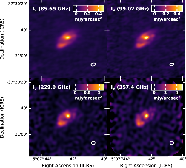
Figure 1: Images of the ALMA 85.69 GHz, 99.02 GHz, 229.9 GHz and 357.4 GHz continuum in the central 60 arcsec of NGC 1808. In each panel, the restoring beam is illustrated as the white open ellipse at the lower-right side.

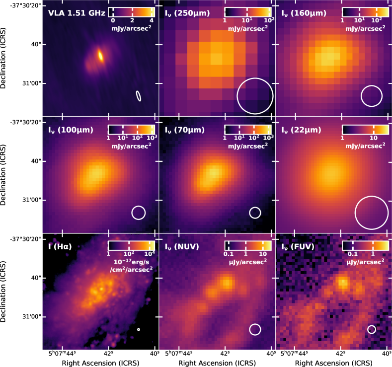
Figure 2: Multiwaveband images of the VLA 1.51 GHz continuum, Herschel 250 $\mu$m, 160 $\mu$m, 100 $\mu$m and 70 $\mu$m continuum, WISE 22 $\mu$m continuum, MUSE H$\alpha$ line, and GALEX NUV and FUV continuum emission in the central 60 arcsec of NGC 1808.

The images of ALMA observations in the central 60 arcsec of NGC 1808 are displayed in the Figure 1. The 85.69 GHz and 99.02 GHz continuum emission are mainly produced by photoionized gas (see more in Section 4) and unaffected by dust obscuration. These two images show that the star formation is mainly concentrated in the nucleus, but several other star-forming regions (e.g., the southeastern one) also produce continuum emission detectable by ALMA. The 229.9 GHz and 357.4 GHz continuum emission are dominated by thermal dust emission (Section 4), but they also trace structures that are similar to what is seen in the 85.69 GHz and 99.02 GHz images at comparable spatial resolution. This is probably because the dust within the central NGC 1808 absorbed the energy from the star-forming regions that are traced by the ALMA Band 3 continuum emission.

The images of other star formation tracers within the centre of NGC 1808 are displayed in the Figure 2. The morphologies differ among these bands.

The nuclear and extended emission is also visible in the 1.51 GHz continuum images. Although the orientation of the beam in the 1.51 GHz image differs from the beam of the ALMA images, the structures in the ALMA and VLA data are largely identical.

The beam sizes of the infrared images shown in Figure 2 are much larger than those of the other images used in this analysis. The beams are so large in the 22 and 250$\mu$m images that the central structure is unresolved. In the 70, 100, and 160 $\mu$m data, however, extended structures can be seen that are similar to what is seen in the ALMA data, although these structures are more poorly resolved in these infrared data.

The last three panels of Figure 2 show images of the MUSE H$\alpha$ line emission and the GALEX ultraviolet continuum emission, which can directly trace the young stellar populations, similar to free-free emission. However, their morphologies appear different from those of the millimetre continuum emission because they are heavily affected by dust obscuration in the centre of the galaxy. This is indicated by the $\hbox{H$\alpha$}/\hbox{H$\beta$}$ flux ratio of $\sim$7 and FUV$-$NUV colour of $\sim$1.7 within the central 1 kpc region, both of which are significantly higher than what is found in nearby star-forming galaxies (Kennicutt et al., 2009; Hao et al., 2011). Compared to the millimetre continuum emission, the H$\alpha$ line emission traces a more extended disc that includes the nucleus and multiple sources of comparable brightness, while the ultraviolet continuum emission traces a few unresolved bright sources and an arc structure. The ultraviolet continuum emission from the galactic center is heavily obscured, but strong emission is seen from two neighbouring sources. The brightest ultraviolet source, which is located $\approx 4$ arcsec (180 pc) northwest from where the millimetre continuum emission peaks, has a counterpart in H$\alpha$ line emission but not in millimetre continuum emission. This location appears to be relatively unobscured, which would explain why the region produces strong ultraviolet emission, but at the same time, the SFR in the region may be relatively low, which would explain the relatively weak millimetre emission. The millimetre-bright southern star-forming region corresponds to a relatively modest, clumpy H$\alpha$ source but not to any ultraviolet source.

3.2 ALMA spectra

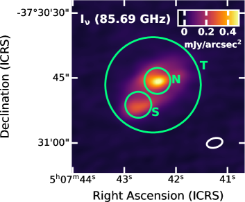
Figure 3: The image of 85.69 GHz continuum emission in the central 40 arcsec of NGC 1808. The solid green circles identify the locations where we extracted spectra, including the total (T), nucleus (N) and south (S) apertures with diameters of 22 arcsec (1 kpc) , 6 arcsec (280 pc) and 6 arcsec (280 pc). The restoring beam is shown as the white open ellipse in the lower-right corner.

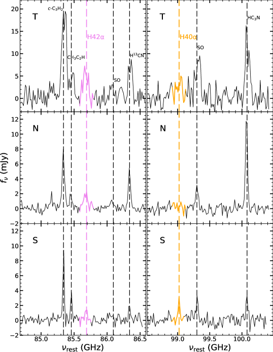
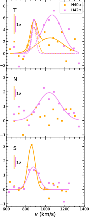
Figure 4: Spectra for the regions illustrated in Figure 3. The left and middle panels show the spectra measured within the entire spectral windows. The frequencies have been separately shifted to the rest frame using the velocities of 990, 990 and 860 $\,{\rm km\,s}^{-1}$ for the T, N and S regions (see text for the measurement). The dashed lines mark the locations of the H42$\alpha$ (purple) and H40$\alpha$ (orange) line emission. The panels on the right show the spectra in detail at the locations of the H40$\alpha$ and H42$\alpha$ lines. The solid lines for the T region (top) show the best fit with two Gaussian functions, and the dotted lines show the individual Gaussian components in these fits. The solid lines for the N region (middle) and S region (bottom) show the profiles fit with single Gaussian functions for the recombination lines. The parameters for all of these functions are listed in Table 5.

Figure 3 shows the locations where we extracted spectra for analysis of the recombination lines. Two measurement apertures with diameters of 6 arcsec (280 pc) were centred on the nucleus (N) and the bright continuum source to the south (S). A third measurement aperture (T) with a diameter of 22 arcsec (1 kpc) was used to measure the total detectable emission from the central region.

Figure 4 shows the spectra of H40$\alpha$ and H42$\alpha$ lines extracted from these three regions. These spectral also reveal the presence of multiple other molecular lines, including $c$-C₃H₂, CH₃C₂H, SO and H¹³CN in the lower frequency spectral window and SO and HC₃N in the higher frequency spectral window. We used single Gaussian functions to fit the CH₃C₂H and H¹³CN lines, which are the most significant line emission in their spectra windows, and obtained average relativistic velocities of $990\pm 10$ $\,{\rm km\,s}^{-1}$ and $860\pm 10$ $\,{\rm km\,s}^{-1}$ for the N and S regions, which we used to shift the frequencies to the rest frame. We also adopted 990 $\,{\rm km\,s}^{-1}$ as the rest frequency for the T region.

Significant H42$\alpha$ line emission is detected in both the N and S regions, and the emission can be fit by single Gaussian functions. The mean relativistic velocity ($v_{0}$) measured in the S region is $\approx$160 $\,{\rm km\,s}^{-1}$ lower that that of the N region. This difference produces a double-peaked line profile in the T region, which we have fitted with two Gaussian functions.

H40$\alpha$ line emission is detected in the S region, and this emission can be described by a single Gaussian function as well. However, no significant H40$\alpha$ line emission is detected in the N region; the signal is lower than the rms noise. We also fit the profile of the H40$\alpha$ line in the T region using two Gaussian functions. The parameters for these Gaussian functions are listed in Table 5.

Table 5: Parameters for Gaussian functions fit to the H42$\alpha$ and H40$\alpha$ lines.

		H42$\alpha$		H40$\alpha$
Region	Component	$v_{0}$	FWHM	$v_{0}$	FWHM
		($\,{\rm km\,s}^{-1}$)	($\,{\rm km\,s}^{-1}$)	($\,{\rm km\,s}^{-1}$)	($\,{\rm km\,s}^{-1}$)
Total	lower $v_{0}$	880 $\pm$ 40	50 $\pm$ 50	880 $\pm$ 20	90 $\pm$ 60
	higher $v_{0}$	1070 $\pm$ 30	240 $\pm$ 70	1050 $\pm$ 90	300 $\pm$ 190
Nucleus	single	1040 $\pm$ 20	260 $\pm$ 50	/	/
South	single	880 $\pm$ 10	130 $\pm$ 30	860 $\pm$ 10	90 $\pm$ 10

It is strange that the H40$\alpha$ line emission is detected in the S region but not the N region while the H42$\alpha$ line emission is detected in both. Notably, in the N region, the noise in the spectrum of the H40$\alpha$ line is approximately twice as larger as the noise in the spectrum of the H42$\alpha$ line. It may be possible the H40$\alpha$ line is not detected in this region simply because of the higher noise levels and the relatively low line flux. However, other scenarios could explain why H42$\alpha$ emission but not H40$\alpha$ emission is detected. We discuss these scenarios below.

The first scenario is that the H40$\alpha$ line emission cannot be detected in the N region because of calibration errors or other related technical issues. However, the H40$\alpha$ emission is still detected in the S region with an integrated signal-to-noise level that is comparable to the H42$\alpha$ emission, which would be difficult to achieve if the H40$\alpha$ line specifically was affected by calibration issues. It therefore seems unlikely that any observing or data processing issues affected the H40$\alpha$ line from the nuclear (N) region specifically.

The second scenario is that the H42$\alpha$ emission from the nucleus is unusually enhanced. The analysis from Gordon & Walmsley (1990) indicates that the H40$\alpha$ and H42$\alpha$ emission should be spontaneous emission and that nonlinear effects should only gradually appear in higher order lines starting with H50$\alpha$. With the exception of a claim by Báez-Rubio et al. (2018) that the H26$\alpha$ emission exhibits masing from a subregion in NGC 253 but H30$\alpha$ does not (in a location on the edge of a much brighter source, which makes the analysis difficult), no one has reported observations of strongly enhanced emission in specific individual recombination lines in any extragalactic sources. It would therefore seem unlikely that such an unusual jump in flux from H40$\alpha$ to H42$\alpha$ emission in the nucleus of NGC 1808 could be explained by line-specific nonlinear effects.

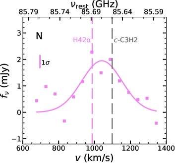
Figure 5: Spectra of the H42$\alpha$ line for the N region illustrated in Figure 3. The gray dashed line shows the location of the $c$-C₃H₂ ($4_{32}$$\rightarrow$$4_{23}$) line.

The last scenario is that the line emission at $\sim$ 85.69 GHz from the galactic nucleus is blended with other spectral lines. The H42$\alpha$ line in the N region has a FWHM approximately twice the FWHM of the molecular lines in the same spectra window (e.g., $c$-C₃H₂, CH₃C₂H, and H¹³CN). While it is possible that the velocity dispersion of the ionized gas is higher than for the molecular gas in that region, it is also possible that the higher FWHM is indicative that the H42$\alpha$ line is blended with another line. Figure 5 shows that the $4_{32}$$\rightarrow$$4_{23}$ transition of $c$-C₃H₂ at 85.65 GHz is close to the frequency of the H42$\alpha$ line. The much stronger $2_{12}$$\rightarrow$$1_{01}$ transition of $c$-C₃H₂ is detected at a rest frequency of 85.34 GHz (the left column of panels in Figure 4). In the starburst/AGN composite galaxy, NGC 4945, Henkel et al. (2018) and Emig et al. (2020) have found that the H42$\alpha$ line emission is probably blended with the $c$-C₃H₂ ($4_{32}$$\rightarrow$$4_{23}$) line, and this contamination effect may increase the flux density by a factor of between $\sim$ 1.1 to 1.6 based on different assumptions. If the H42$\alpha$ emission is blended with $c$-C₃H₂ emission in the nucleus of NGC 1808, the combined line emission could have been easier to detect than the H40$\alpha$ emission. However, the two lines are so close that it is difficult to either confirm or quantify the relative fraction of the emission originating from the $c$-C₃H₂ in our spectra. Additionally, it is unclear if the line ratios estimated from the NGC 4945 are applicable to NGC 1808. If we exclude the channels covering the potential $c$-C₃H₂ ($4_{32}$$\rightarrow$$4_{23}$) line between 85.63 and 85.66 GHz, corresponding to a velocity range of $\sim$ 100 $\,{\rm km\,s}^{-1}$, the H42$\alpha$ line flux will be reduced by $\sim$ 40 per cent, which is broadly consistent with the line flux ratios found in NGC 4945 (Emig et al., 2020). Having said this, the millimeter continuum emission, which is dominated by free-free emission (see in Section 4), clearly peaks in the nucleus, which indicates the presence of the photoionized gas that would be expected to have recombination line emission associated with it. This implies that it is more likely that the line emission at 85.69 GHz is predominantly H42$\alpha$ emission.

Given the discrepancies in the measurements of the H40$\alpha$ and H42$\alpha$ lines from the N region, we will treat quantities calculated from these lines as the lower and upper limits. We also discuss how excluding the channels covering the potential $c$-C₃H₂ emission between 85.63 and 85.66 GHz may affect these quantities.

4 Spectral Energy Distribution

Table 6: Continuum measurements for SED analysis.

Rest frame	Flux density
frequency	T region	N region	S region
(GHz)	(mJy)	(mJy)	(mJy)
1.52	182 $\pm$ 18	60 $\pm$ 6	29 $\pm$ 4
4.91	99 $\pm$ 10	36 $\pm$ 4	16 $\pm$ 2
8.50	46 $\pm$ 5	18 $\pm$ 2	8 $\pm$ 1
86.58	26 $\pm$ 1	8 $\pm$ 0.4	5 $\pm$ 0.3
87.72	28 $\pm$ 1	8 $\pm$ 0.4	6 $\pm$ 0.3
98.55	25 $\pm$ 1	7 $\pm$ 0.4	5 $\pm$ 0.3
100.79	25 $\pm$ 1	7 $\pm$ 0.4	5 $\pm$ 0.3
102.24	24 $\pm$ 1	7 $\pm$ 0.4	5 $\pm$ 0.2
114.24	22 $\pm$ 1	7 $\pm$ 0.3	5 $\pm$ 0.3
219.96	66 $\pm$ 7	19 $\pm$ 2	14 $\pm$ 1
229.86	69 $\pm$ 7	18 $\pm$ 2	16 $\pm$ 2
233.90	71 $\pm$ 7	19 $\pm$ 2	16 $\pm$ 2
245.47	80 $\pm$ 8	22 $\pm$ 2	18 $\pm$ 2
344.95	202 $\pm$ 20	59 $\pm$ 6	49 $\pm$ 5
357.41	249 $\pm$ 25	69 $\pm$ 7	63 $\pm$ 6

For our analysis, we need to identify the fraction of continuum emission in ALMA Band 3 that originates from free-free emission. To do this, we use all the ALMA and VLA continuum data between 1 and 360 GHz in the T, N and S regions to construct SEDs, which we then fit with functions representing synchrotron, free-free, and thermal dust emission. The continuum measurements used in our SED analysis are listed in Table 6. We model the synchrotron emission and thermal dust emission as power laws where the scales and spectral indices are set as free parameters. We use the Gaunt factor ($g_{ff}$) given by Draine (2011) to set the shape of the free–free emission. This function is given as

$$g_{ff}=0.5535\ln\left|\left[\frac{T_{e}}{\mbox{K}}\right]^{1.5}\left[\frac{\nu}{\mbox{GHz}}\right]^{-1}Z^{-1}\right|-1.682.$$ (1)

where $\nu$ is the frequency and $Z$ is the charge of the ions, which is set to 1. The scale of the free-free emission was treated as a free parameter. For fitting the SED, we set $T_{e}$ to 5000 K, which is comparable to the numbers derived in Section 5 as well as to electron temperatures derived in other nearby starburst galaxies (Bendo et al., 2015, 2016); our measurements of the flux density from free-free emission varies by $\leq 5$ per cent when $T_{e}$ varies from 1000 to 10000 K.

Using the lmfit package (Newville et al. 2022), we first used a Levenberg-Marquardt algorithm to fit the SED in a logarithmic space, and then we applied the Maximum likelihood via Monte-Carlo Markov Chain method in 1,000 iterations to sample the posterior distributions of the fitting parameters. Based on the fitting parameters, we calculated the fractions of synchrotron, free-free, and thermal dust emission to the total emission. Our measurements and associated uncertainties are derived from the medians and half the difference between the 15.8 and 84.2 percentiles of the posterior distributions, which is equivalent to the inner 68% of the distributions.

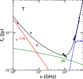
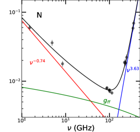
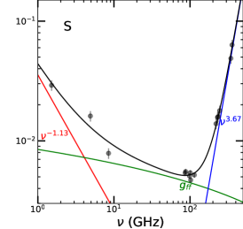
Figure 6: The SEDs for the T, N and S regions of NGC 1808. The black lines show the best fitting SED model for the data. The red lines represent synchrotron emission. The green lines represent free–free emission based on the Gaunt factor with $T_{e}$ fixed at 5000 K. The blue lines correspond to thermal dust emission.

Table 7: SED analysis results.

	Synchrotron emission			Free-free emission		Thermal dust emission
Region	Spectra	Fraction at	Fraction at	Fraction at	Fraction at	Spectra	Fraction at	Fraction at
	index	85.69 GHz (%)	99.02 GHz (%)	85.69 GHz (%)	99.02 GHz (%)	index	85.69 GHz (%)	99.02 GHz (%)
T	$-0.99\pm 0.16$	$12\pm 7$	$10\pm 7$	$83\pm 8$	$81\pm 7$	$3.66\pm 0.18$	$5\pm 1$	$9\pm 2$
N	$-0.74\pm 0.14$	$33\pm 15$	$30\pm 14$	$62\pm 15$	$62\pm 14$	$3.63\pm 0.16$	$5\pm 1$	$8\pm 1$
S	$-1.13\pm 0.20$	$5\pm 4$	$4\pm 3$	$89\pm 4$	$86\pm 4$	$3.67\pm 0.15$	$6\pm 1$	$10\pm 2$

The best fitting parameters from the SED fits are listed in Table 7, and the SEDs and the best-fitting functions are shown in Figure 6. According to the best fitting SED model for the data, the free-free emission dominates between 20 and 150 GHz and produces $\sim$80 per cent of the total observed emission (with an uncertainty of $\lesssim$8 per cent) at the rest frequencies of the H40$\alpha$ and H42$\alpha$ lines, while the synchrotron and dust emission produce the remaining $\sim$20 per cent of the emission. The fraction of the total emission from synchrotron emission is almost seven times greater in the N region than in the S region, which may arise from the presence of the AGN or more supernovae in the galactic nucleus. However, the widths of hydrogen recombination line are $\lesssim 300\,{\rm km\,s}^{-1}$, so even if an AGN is present in the nucleus, it should be a relatively weak energy source.

The spectral indices of the millimetre and radio continuum emission in the centre of NGC 1808 have been explored in several previous studies. Dahlem et al. (1990) reported a mean spectral index of $-0.88$ for the nonthermal radiation in the central starburst based on 20 cm (1.5 GHz) and 6 cm (4.9 GHz) VLA data with a resolution of 20 arcsec. The spectral index of $-0.99\pm 0.16$ that we measured in the T region from our SED analysis is in good agreement with their measurement despite the fact that the data and methodology that we used to estimate the spectral index are different from theirs. This agreement suggests that the synchrotron radiation dominates the 1.5 GHz emission from the central starburst.

Salak et al. (2016) calculated spectra indices at each pixel from 102 and 114 GHz ALMA data and found that the indices varied significantly within the central region, ranging from $-3$ to 1 in the central 2 arcsec diameter region and equalling about $-1$ in the galactic centre. However, these spectra index variations were affected by pixel-to-pixel variations in low signal-to-noise data. Salak et al. (2017) performed a follow-up analysis of the 21 to 350 GHz SED of the central 2 arcsec diameter region using both ALMA and eVLA data, and they determined that 72 per cent of the 93 GHz emission originates from free-free emission, with 22 per cent arising from synchrotron and 6 per cent from dust. The proportions of free-free emission, synchrotron emission and dust emission we measured in the nuclear region are comparable to those presented by Salak et al. (2017), although the relative fractions of synchrotron emission and free-free emission measured by Salak et al. (2017) are about 10 per cent different from our measurements. The variations between these results and ours are probably related to the different spatial resolution of data, the different apertures used to make the measurements, and the different methods used to fit SEDs (e.g., the Gaunt factor for free-free emission and unrestricted spectra indices of synchrotron and dust emission). If we fixed the spectral indices of synchrotron emission and dust emission to the values used by Salak et al. (2017), then we obtained 76 per cent of the 93 GHz emission originating from free-free emission and 19 per cent originating from synchrotron, which are consistent with their measurements.

More recently, Audibert et al. (2021) measured the spectral index from 8 to 93 GHz in the central 2 arcsec diameter region to be $-1$, which they interpreted as consistent with emission originating entirely from synchrotron emission in these bands, and they measured the spectral index from 350 to 500 GHz in the same region to be 3.6, which they used as evidence to indicate that dust emission dominated these bands. Although we also conclude that the emission from 350 to 500 GHz is dominated by dust emission, our results show that the SED bends between 8 and 93 GHz (see Figure 6), which would indicate that using a single spectral index to characterize the emission between these bands, as done by Audibert et al. (2021), will provide an inadequate description of the shape of the SED.

Aside from NGC 1808, the extragalactic SEDs from far-infrared continuum to radio continuum emission have only been published for M82 (Condon, 1992; Peel et al., 2011), NGC 253 (Peel et al., 2011; Bendo et al., 2015), NGC 4945 (Peel et al., 2011; Bendo et al., 2016) and NGC 3256 (Michiyama et al., 2020). Although the proportions measured varied among the galaxies and although different groups obtained slightly different results for specific galaxies, these SED results still demonstrate that the dominant source of continuum emission from 84 to 116 GHz, corresponding to the frequency range of ALMA Band 3, is free-free emission. Our SED results for NGC 1808 are largely consistent with this. Additionally, these results from these other galaxies and our results for NGC 1808 show that dust emission is consistently the dominant source of emission seen in ALMA Bands 6 and 7.

5 Electron Temperatures

The ratio of the hydrogen recombination line emission integrated over velocity $v$, $\int f_{\nu}$(line)$dv$, to the free–free emission, $f_{\nu}$(ff), can be written as

$$\begin{split}\frac{\int f_{\nu}(\mbox{line})dv}{f_{\nu}(\mbox{ff})}\left[\frac{\mbox{Jy}}{\mbox{Jy km s}^{-1}}\right]=\ \ \ \ \ \ \ \ \ \ \ \ \ \ \ \ \ \ \ \ \ \ \ \ \ \ \ \ \ \ \ \ \ \ \ \ \ \ \ \ \ \ \ \ \ \ \ \ \\ 4.38\times 10^{33}g_{ff}^{-1}\left[\frac{\epsilon_{\nu}}{\mbox{erg s}^{-1}\mbox{ cm}^{-3}}\right]\left[\frac{\nu}{\mbox{~{}GHz}}\right]^{-1}\left[\frac{T_{e}}{\mbox{~{}K}}\right]^{0.5},\end{split}$$ (2)

which we can use to derive electron temperatures ($T_{e}$), as presented by Bendo et al. (2016) based on equations from Draine (2011) and Scoville & Murchikova (2013). $\epsilon_{\nu}$ is the emissivity from Storey & Hummer (1995), and while it does not change significantly as a function of electron density ($n_{e}$) between $10^{2}$ and $10^{5}$ cm^-3, it varies strongly as a function of $T_{e}$ in the range of 500-30000 K. We therefore use $\epsilon_{\nu}$ corresponding to case B recombination with a fixed $n_{e}$ value of $10^{3}$ cm^-3 but interpolate $\epsilon_{\nu}$ for different $T_{e}$. In addition, $g_{ff}$ is also allowed to vary with $T_{e}$ for our analysis, although the maximum variation of $g_{ff}$ with $T_{e}$ is only $\sim 2\times$ over the range of 2000-20000 K. Two separate electron temperature measurements are made based on the two separate spectral lines.

Table 8: $T_{e}$ analysis results.

Region	85.69 GHz	H42$\alpha$	H42$\alpha$	$T_{e}$	99.02 GHz	H40$\alpha$	H40$\alpha$	$T_{e}$
	free–free	line	line/free-free	from H42$\alpha$	free–free	line	line/free-free	from H40$\alpha$
	flux density	flux	emission ratio	line/free-free	flux density	flux	emission ratio	line/free-free
	(mJy)	(mJy $\,{\rm km\,s}^{-1}$)	(mJy $\,{\rm km\,s}^{-1}$ mJy-1)	(K)	(mJy)	(mJy $\,{\rm km\,s}^{-1}$)	(mJy $\,{\rm km\,s}^{-1}$ mJy-1)	(K)
T	$26\pm 2$	$1610\pm 170$	$63\pm 9$	$3800\pm 500$	$23\pm 2$	$980^{\star}\pm 200$	$42\pm 9$	$6400^{\star}\pm 1500$
N	$5\pm 1$	$420\pm 30$	$81\pm 20$	$3000\pm 700$	$5\pm 1$	$90^{\star}\pm 50$	$18\pm 11$	$13700^{\star}\pm 8000$
S	$5\pm 0.2$	$200\pm 30$	$40\pm 6$	$5700\pm 900$	$5\pm 0.2$	$270\pm 40$	$57\pm 9$	$4900\pm 700$

^⋆ These values are affected by the non-detected H40$\alpha$ line emission in the N region.

Note. These line flux and free-free flux density measurements do not include calibration uncertainties, as the ratios and the $T_{e}$ derived from the ratios should be independent of the calibration. However, the uncertainties in the fraction of continuum emission that originates from free-free emission are incorporated into these data.

Table 8 lists all the free-free flux densities, spectra line fluxes and electron temperatures measured in the three regions shown in Figure 3. The spectra line fluxes are directly measured from the data (and not based on Gaussian fits). To integrate the flux for the H42$\alpha$ lines in each spectra and for the H40$\alpha$ line in the S spectrum, we selected channels that would give line fluxes with optimized signal-to-noise ratios; the relativistic velocity widths covered by the channels in the T, N, and S spectra are 350 $\,{\rm km\,s}^{-1}$, 250 $\,{\rm km\,s}^{-1}$ and 150 $\,{\rm km\,s}^{-1}$. For the H40$\alpha$ lines in the T and N spectra, which have a low signal-to-noise, we used the same velocity ranges as used for the H42$\alpha$ line. The free-free flux densities and spectra line fluxes within the N and S regions are approximately 40 per cent of that within the T region, which implies that the central 1 kpc diameter region also encompasses additional fainter star-forming regions.

The $T_{e}$ measured in the T region is 6400 K based on the H40$\alpha$/99.02 GHz free-free emission ratio but only 3800 K based on the H42$\alpha$/86.59 GHz free-free emission ratio. The difference of $T_{e}$ arises from the missing H40$\alpha$ line emission in the N region, as discussed in Section 3.2. If we remove the channels covering the $c$-C₃H₂ ($4_{32}$$\rightarrow$$4_{23}$) line (using 100 $\,{\rm km\,s}^{-1}$ for the assumed line width), the electron temperatures from the H42$\alpha$/86.59 GHz free-free continuum ratio will increase to $5900\pm 1000$ K and $4700\pm 1100$ K for the T and N regions, respectively. Since the $T_{e}$ values measured from the N region are not robust, we will not rely on them for the rest of our analysis. We therefore use the average electron temperature of $5200\pm 500$ K from the T and S regions in the calculation of SFRs in Section 6.

The average electron temperature for the central starburst of NGC 1808 is comparable to that of the central region of the Milky Way (e.g., Shaver et al., 1983; Paladini et al., 2004), the central starburst of NGC 4945 (Bendo et al., 2016) and the northern starburst nucleus of NGC 3256 (Michiyama et al., 2020), while it is slightly higher than that of the centre of NGC 253 (Bendo et al., 2015). If we assume only half of the 86.59 GHz continuum emission originated from free-free emission, then the resulting electron temperature from the T region would be $\sim 2300$ K, which seems unreasonably low compared to that of nearby galaxies. We can therefore infer that the free-free emission comprises more than half of the total 85.69 GHz continuum emission for the central starburst of NGC 1808.

6 Star Formation Rates

6.1 SFR measurements from ALMA data

The SFR can be calculated from the photoionizing photon production rate ($Q$) using

$$\frac{\mbox{SFR}}{\mbox{M}_{\odot}~{}\mbox{yr}^{-1}}=7.29\times 10^{-54}\frac{Q}{\mbox{s}^{-1}},$$ (3)

where the conversion was derived from Murphy et al. (2011) using the Starburst99 model (Leitherer et al., 1999) with solar metallicity ($Z_{\odot}$ = 0.020), a Kroupa (2002) initial mass function (IMF) for a mass range of $0.1-100$ M_⊙ and no stellar rotation. While different conversions that account for the stellar rotation from Leitherer et al. (2014) were used in previous studies (Bendo et al., 2015, 2016; Bendo et al., 2017), these conversions are not widely used and also produce significantly different SFRs from other conversion equations. To simplify our comparison of SFRs, we use a standard conversion that includes no rotation effects.

The hydrogen recombination line emission integrated over velocity and free–free emission can be related to the values to $Q$ by applying

$$Q=\alpha_{B}n_{e}n_{p}V$$ (4)

from Scoville & Murchikova (2013). $\alpha_{B}$ is the effective recombination coefficient from Storey & Hummer (1995), which varies strongly with $T_{e}$, but changes little for $n_{e}$ values ranging from $10^{2}$ to $10^{5}$ cm^-3. We therefore keep the electron density $n_{e}$=$10^{3}$ cm^-3 constant and use an $\alpha_{B}$ corresponding to the $T_{e}$ value of 5200 K, which is the average derived from the T and S region in Section 5. Following this, we can convert the free-free and recombination line emission to SFRs using

$$\begin{split}\frac{\mbox{SFR}(\mbox{ff})}{\mbox{M}_{\odot}\mbox{ yr}^{-1}}=1.28\times 10^{11}\ \ \ \ \ \ \ \ \ \ \ \ \ \ \ \ \ \ \ \ \ \ \ \ \ \ \ \ \ \ \ \ \ \ \ \ \ \ \ \ \ \ \ \ \ \ \ \ \ \ \ \ \\ \times g_{ff}^{-1}\left[\frac{\alpha_{B}}{\mbox{ cm}^{3}\mbox{ s}^{-1}}\right]\left[\frac{T_{e}}{\mbox{~{}K}}\right]^{0.5}\left[\frac{D}{\mbox{ Mpc}}\right]^{2}\left[\frac{f_{\nu}(\mbox{ff})}{\mbox{Jy}}\right]\end{split}$$ (5)

and

$$\begin{split}\frac{\mbox{SFR}(\mbox{line})}{\mbox{M}_{\odot}\mbox{ yr}^{-1}}=2.91\times 10^{-23}\left[\frac{\alpha_{B}}{\mbox{ cm}^{3}\mbox{ s}^{-1}}\right]\ \ \ \ \ \ \ \ \ \ \ \ \ \ \ \ \ \ \ \ \ \ \ \ \ \ \ \ \ \ \\ \times\left[\frac{\epsilon_{\nu}}{\mbox{erg s}^{-1}\mbox{ cm}^{-3}}\right]^{-1}\left[\frac{\nu}{\mbox{~{}GHz}}\right]\left[\frac{D}{\mbox{ Mpc}}\right]^{2}\left[\frac{\int f_{\nu}(\mbox{line})dv}{\mbox{Jy km s}^{-1}}\right],\end{split}$$ (6)

where $D$ is the distance, and $f_{\nu}$(ff) and $\int f_{\nu}$(line)$dv$ are listed Table 8. Because the two different hydrogen line measurements from the galactic nucleus yield different results, SFR(line) is calculated only for comparison to SFR(ff).

Table 9: SFR measurments from ALMA data.

Region	85.69 GHz	H42$\alpha$	99.02 GHz	H40$\alpha$
	free-free	line	free-free	line
	(M⊙ yr-1)	(M⊙ yr-1)	(M⊙ yr-1)	(M⊙ yr-1)
T	$3.2\pm 0.4$	$4.5\pm 0.7$	$3.0\pm 0.4$	$2.4^{a}\pm 0.6$
N	$0.63\pm 0.16$	$1.16\pm 0.15$	$0.63\pm 0.15$	$<0.65^{b}$
S	$0.62\pm 0.05$	$0.55\pm 0.10$	$0.59\pm 0.05$	$0.64\pm 0.11$

^a This value is affected by the non-detected H40$\alpha$ line emission.

^b This upper limit is estimated with 5$\sigma$ uncertainty.

The final SFRs measured from the ALMA data are listed in Table 9. The average of the free-free SFRs integrated over the central starburst (T region) is $3.1\pm 0.3$ M_⊙ yr^-1; we use this average later in comparisons to SFRs from other bands. While the area of the combined N and S regions is only 15 per cent of the T region, the emission from these two regions contributes approximately 40 per cent of the total SFR in the central starburst.

The total SFR within the central starburst is broadly consistent with the recent published SFR of $2.5-3.5$ M_⊙ yr^-1 within the central 30 arcsec region using the ALMA 93 GHz emission, which they treat as dominated by free–free emission (Salak et al., 2017); the SFR values have been rescaled for a distance of 9.5 Mpc for comparison to our measurements. In addition, Salak et al. (2017) also measured an SFR of $0.16-0.22$ M_⊙ yr^-1 in a 2 arcsec aperture. Given the difference in aperture size, the nuclear SFR of $0.63$ M_⊙ yr^-1 that we obtained in an 6 arcsec aperture is broadly comparable to their measurement.

After deriving the SFR from the millimetre data, we calculated SFRs from radio, infrared, H$\alpha$ and ultraviolet data using the same Starburst99 model with the Kroupa (2002) IMF. Since the beam FWHMs in the infrared data are significantly larger than the aperture sizes of the N and S regions, we only compared the SFRs measured from multi wavebands within the central 1 kpc starburst (T region).

Table 10: SFR measurements for the central 1 kpc in NGC 1808.

SFR Metrics	Flux or flux density	SFR (M⊙ yr-1)
85.69 GHz free-free	$26\pm 2$ mJy	$3.2\pm 0.4$
H42$\alpha$ line	$1.6\pm 0.2$ Jy$\,{\rm km\,s}^{-1}$	$4.5\pm 0.7$
99.02 GHz free-free	$23\pm 2$ mJy	$3.0\pm 0.4$
H40$\alpha$ line	$1.0^{\star}\pm 0.2$ Jy$\,{\rm km\,s}^{-1}$	$2.3^{\star}\pm 0.6$
1.5 GHz continuum	$344\pm 34$ mJy	$2.3\pm 0.2$
TIR continuum	$8.7\pm 0.5\times 10^{14}$ Jy Hz	$3.6\pm 0.2$
160 $\mu$m infrared continuum	$86\pm 7$ Jy	$2.4\pm 0.2$
70 $\mu$m infrared continuum	$122\pm 7$ Jy	$3.3\pm 0.2$
22 $\mu$m infrared continuum	$11.9\pm 0.7$ Jy	$3.6\pm 0.2$
H$\alpha$ (corrected using TIR)	$2.2\pm 0.1\times 10^{12}$ Jy Hz	$1.3\pm 0.1$
H$\alpha$ (corrected using 22 $\mu$m)	$3.4\pm 0.2\times 10^{12}$ Jy Hz	$2.0\pm 0.1$
NUV (corrected using TIR)	$2.4\pm 0.1\times 10^{14}$ Jy Hz	$1.7\pm 0.1$
NUV (corrected using 22 $\mu$m)	$3.7\pm 0.2\times 10^{14}$ Jy Hz	$2.7\pm 0.2$
FUV (corrected using TIR)	$4.0\pm 0.2\times 10^{14}$ Jy Hz	$1.9\pm 0.1$
FUV (corrected using 22 $\mu$m)	$6.3\pm 0.4\times 10^{14}$ Jy Hz	$3.0\pm 0.2$

^⋆ These values are affected by the non-detected H40$\alpha$ line emission.

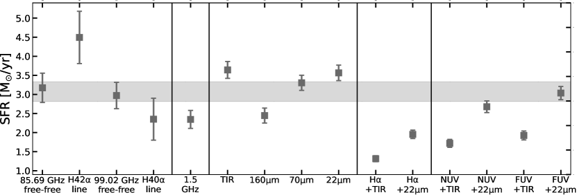
Figure 7: SFR measurements for the central starburst in NGC 1808 (T region). The grey shaded region corresponds to the mean within 1$\sigma$ uncertainties of SFRs from the H42$\alpha$ line and 85.69 GHz free-free emission.

All of the SFR measurements for the central starburst in NGC 1808 are summarized in Table 10 and illustrated in Figure 7. In the following sections, we will discuss the comparisons of the SFR measurements from ALMA and the SFR measurements from radio, infrared, H$\alpha$ and ultraviolet data specifically.

6.2 Comparisons of ALMA and radio SFRs

For calculating SFRs based on the radio flux density, we use the integrated measurement in the T aperture of $344\pm 34$ mJy from the 1.5 GHz VLA data (Section 2.2) and

$$\frac{\mbox{SFR}(1.5\mbox{GHz})}{\mbox{M}_{\odot}\mbox{ yr}^{-1}}=0.0760\left[\frac{D}{\mbox{Mpc}}\right]^{2}\left[\frac{f_{\nu}(1.5\mbox{ GHz})}{\mbox{Jy}}\right]$$ (7)

given by Murphy et al. (2011), and we obtained an SFR of $2.3\pm 0.2$ M_⊙ yr^-1.The SFR estimated from the 1.5 GHz emission is approximately 75 per cent of the SFR from the free-free emission; the difference between the two values is $\sim$2$\sigma$. This difference was most likely caused by the diffusion through the interstellar medium of the cosmic rays producing the synchrotron radiation (e.g., Murphy et al., 2006), which would make the radio emission appear broad compared to other star formation tracers. In addition, if a radio-emitting AGN is present in the galactic nucleus, the SFR from radio emission that we calculated could be expected to be much higher than what we derived from the free-free emission. Since the SFR from the 1.5 GHz band is lower than what we get from free-free emission, this implies that the AGN is not a significant energy source in radio bands.

6.3 Comparisons of ALMA and infrared SFRs

6.3.1 Infrared photometry

Unlike millimetre and radio data, infrared emission is seen in a compact central region as well as diffuse structures distributed throughout the optical disc (Figure 2). As a consequence, we need to remove this extended emission by applying local background subtractions when performing the measurements. In addition, we need to apply the aperture corrections to the infrared flux densities because the infrared data is not well resolved, even in the T region.

In the WISE 22 $\mu$m image, we followed the procedures used in the WAPPco photometry system to produce the WISE All-Sky Data Release Products. We first measured the target flux density from a 22 arcsec aperture corresponding to the T region. After this, we subtracted the median background within an annulus with radii of 50–70 arcsec and applied an aperture correction of 2.77 that, based on the WISE beam provided by Cutri et al. (2013), is appropriate for this target and background aperture combination. No colour correction is needed in WISE 22 $\mu$m data because this effect is negligible ( $<$$\sim$1 per cent) from unity for power law spectra ranging from $\nu^{-3}$ to $\nu^{3}$ (Wright et al., 2010). Following these calculations, we obtained a 22 $\mu$m flux density of $11.9\pm 0.7$ Jy.

In the PACS 70, 100 and 160 $\mu$m images, we first measured the target flux densities within the 22 arcsec apertures, subtracted the median background measured within annuli with radii of 61-70 arcsec and multiplied by aperture correction factors of 1.26, 1.32 and 1.52, which come from the PACS Ancillary Data Products (Lutz, 2015). Next, we multiplied our measurements by colour correction factors of 1.06, 1.00 and 1.03 (corresponding to the PACS 70, 100 and 160 $\mu$m bands, respectively), which were derived by Bendo et al. (2016) from values given by Müller et al. (2011) for modified blackbodies with emissivities scaling as either $\nu$ or $\nu^{2}$ and with temperatures ranging from 20 to 50 K. Following this, we obtained flux densities of $122\pm 7$, $128\pm 8$ and $86\pm 7$ Jy at 70, 100 and 160 $\mu$m, respectively.

In the SPIRE 250 $\mu$m image, we first measured the target flux densities from the aperture with a radius of 22 arcsec, and then subtracted the median background within an annulus with radii of 30-60 arcsec. Following the SPIRE Data Reduction Guide (Centre, 2016), we multiplied this value by an aperture correction of 1.27. Next, we multiplied the flux density by the colour correction factor of 0.955 for SPIRE 250 $\mu$m dust emission given by Bendo et al. (2016), who derived this factor based on values from the SPIRE Handbook (Valtchanov et al., 2018) for point-like modified blackbodies with emissivity indices of $\nu^{-1.5}$ or $\nu^{-2}$ and temperatures ranging from 15 to 40 K. We obtained a final 250 $\mu$m flux density of $32.5\pm 1.8$ Jy.

6.3.2 Comparison of ALMA and total infrared SFRs

Using the infrared measurements from 22 $\mu$m to 500 $\mu$m and

$$\begin{split}F(\mbox{TIR})=2.023\nu f_{\nu}(22\mu\mbox{m})+0.523\nu f_{\nu}(70\mu\mbox{m})\ \ \ \ \ \ \ \ \ \ \ \ \ \ \ \ \ \ \ \ \ \ \ \ \\ +0.390\nu f_{\nu}(100\mu\mbox{m})+0.577\nu f_{\nu}(160\mu\mbox{m})+0.721\nu f_{\nu}(250\mu\mbox{m})\end{split}$$ (8)

given by Galametz et al. (2013), we obtained a total infrared (TIR) flux of $8.7\pm 0.5\times 10^{14}$ Jy Hz, equivalent to a TIR luminosity of $2.5\pm 0.2\times 10^{10}L_{\odot}$. Using the conversion

$$\frac{\mbox{SFR}(\mbox{TIR})}{\mbox{M}_{\odot}\mbox{ yr}^{-1}}=4.66\times 10^{-17}\left[\frac{D}{\mbox{Mpc}}\right]^{2}\left[\frac{F(\mbox{TIR})}{\mbox{Jy Hz}}\right]$$ (9)

from Murphy et al. (2011), we obtain an SFR of $3.6\pm 0.2$ M_⊙ yr^-1.

The TIR flux yields an SFR approximately 15 per cent (or 2 $\sigma$) higher than the ALMA free-free SFR. Given the uncertainties of the infrared photometry as well as the additional uncertainties in the TIR flux calculation (typically 4 per cent but potentially higher; Galametz et al., 2013), the difference is not significant.

The assumption behind using the TIR flux to calculate SFR is that the TIR flux probes the emission absorbed and re-radiated by dust from star-forming regions that produce most of the bolometric luminosity of galaxies. Additionally, Kennicutt & Evans (2012) indicate that the conversion between TIR flux and SFR depends on the relative fraction of the stellar emission that is absorbed by dust. The conversion from Murphy et al. (2011) is based on dust absorbing all energy shortwards of the Balmer break at 3646 Åbut not at longer wavelength. However, in very dusty regions like the centre of NGC 1808, a significant fraction of the starlight at longer wavelengths may also be absorbed, thus leading to overestimated SFRs from the TIR.

Other non-photoionizing stars, ranging from ultraviolet-bright stars with ages just over 10 Myr to much older evolved red stars, may also heat interstellar dust (e.g., Hao et al., 2011). However, in the centre of NGC 1808, our results indicate that energy absorbed by dust from those stars would produce 15 per cent of the TIR emission. Additionally, energy absorbed by interstellar dust from evolved stars would tend to be emitted at longer wavelengths (e.g., Kennicutt, 1998), but the SFR calculated from the 160 $\mu$m data is relatively low in comparison (see Section 6.3.3), which implies that dust heating by evolved stars is not significant.

An AGN could also potentially produce additional infrared emission. However, if an AGN were the dominant infrared emission source in this galaxy, then the TIR SFR would be expected to be much higher than the ALMA SFR. Since the discrepancy between TIR SFR and ALMA SFR is only 15 per cent, and the SFR from the TIR emission is 1.5 times higher than the SFR from the 1.5 GHz emission (which would also be expected to be high if an AGN were present), we can conclude that any AGN that is present produces a relatively small fraction of the total infrared emission from NGC 1808 and that star-forming regions are the main source of infrared emission from this galaxy.

6.3.3 Comparisons of ALMA and monochromatic infrared SFRs

Beside the conversion from TIR emission to SFR, several conversions from monochromatic infrared dust emission to SFR are also widely used. The conversion from WISE 22 $\mu$m emission to SFR is the same as that from other mid-infrared data (e.g., Lee et al., 2013). Using one of the most widely used relations,

$$\frac{\mbox{SFR}(22\mu\mbox{m})}{\mbox{M}_{\odot}\mbox{ yr}^{-1}}=2.44\times 10^{-16}\left[\frac{D}{\mbox{Mpc}}\right]^{2}\left[\frac{\nu f_{\nu}(22\mu\mbox{m})}{\mbox{Jy Hz}}\right]$$ (10)

given by Rieke et al. (2009), we obtained an SFR of $3.6\pm 0.2$ M_⊙ yr^-1. In this case, the corresponding mid-infrared luminosity is $4.6\pm 0.3\times 10^{9}\mbox{L}_{\odot}$, which falls within the range of $6\times 10^{8}$ to $1.3\times 10^{10}\mbox{L}_{\odot}$ over which this relation should be applicable.

The 70 $\mu$m and 160 $\mu$m measurements can also be used to calculate SFRs. Using

$$\frac{\mbox{SFR}(70\mu\mbox{m})}{\mbox{M}_{\odot}\mbox{ yr}^{-1}}=7.04\times 10^{-17}\left[\frac{D}{\mbox{Mpc}}\right]^{2}\left[\frac{\nu f_{\nu}(70\mu\mbox{m})}{\mbox{Jy Hz}}\right]$$ (11)

and

$$\frac{\mbox{SFR}(160\mu\mbox{m})}{\mbox{M}_{\odot}\mbox{ yr}^{-1}}=1.71\times 10^{-16}\left[\frac{D}{\mbox{Mpc}}\right]^{2}\left[\frac{\nu f_{\nu}(160\mu\mbox{m})}{\mbox{Jy Hz}}\right]$$ (12)

from Calzetti et al. (2010), we obtained an SFR$(70\mu\mbox{m})$ of $3.3\pm 0.2$ M_⊙ yr^-1 and an SFR$(160\mu\mbox{m})$ of $2.4\pm 0.2$ M_⊙ yr^-1 for the central 1 kpc region. In this case, the corresponding 70 $\mu$m and 160 $\mu$m luminosities are of $1.5\pm 0.1\times 10^{10}\mbox{L}_{\odot}$ and $4.5\pm 0.4\times 10^{9}\mbox{L}_{\odot}$, both of which fall within the ranges where these relations should apply.

The 22 $\mu$m and 70 $\mu$m flux densities yield SFRs 20 per cent and 10 per cent higher than the ALMA SFR, while the 160 $\mu$m flux density yields an SFR 17 per cent lower than the ALMA SFR. The conversions from monochromatic infrared emission to SFR are based on assumptions that the shape of infrared SED remains unchanged and that the monochromatic infrared emission scales linearly with the TIR emission (as well as the additional assumptions involved in converting from TIR emission to SFR). Considering the calibration uncertainties of the conversions are 0.2 dex, 0.2 dex and 0.4 dex for 22  $\mu$m, 70 $\mu$m and 160 $\mu$m emission, respectively (Rieke et al., 2009; Calzetti et al., 2010), the discrepancies among these SFRs or between them and the ALMA free-free SFR are not significant.

However, the calculated SFR still decreases notably with wavelength. This relation may arise because the dust within NGC 1808 is relatively hot compared to the star-forming and starburst galaxies used by Calzetti et al. (2010). This trend has also been found in NGC 5253, which is a dwarf starburst galaxy with abnormally hot dust (Bendo et al., 2017).

6.4 Comparisons of ALMA, PAH and Br$\gamma$ SFRs

Some researchers have proposed using polycyclic aromatic hydrocarbon (PAH) emission to measure the SFR (e.g., Diamond-Stanic & Rieke, 2010, 2012), which would be advantageous for measuring SFRs in locations where AGN produce much of the bolometric luminosity. In NGC 1808, Esquej et al. (2014) measured an SFR of $0.55M_{\odot}$ yr^-1 (rescaled for a distance of 9.5 Mpc) from the 11.3 $\mu$m PAH emission in an aperture comparable to our T region. This is $\sim$5$\times$ lower than the SFRs from our ALMA and infrared data. PAH emission is generally expected to be suppressed relative to hot dust emission and other commonly used star formation tracers, most likely because the PAHs are more easily destroyed by the hard ultraviolet radiation fields in star-forming regions (e.g., Helou et al., 2004; Calzetti et al., 2005, 2007; Bendo et al., 2006, 2008; Povich et al., 2007; Lebouteiller et al., 2007; Prescott et al., 2007; Jones et al., 2015; Egorov et al., 2023). Even though the PAH 11.3 $\mu$m feature specifically was expected to be a more robust star formation tracer than other PAH lines (Diamond-Stanic & Rieke, 2010), it works poorly as an SFR metric in the centre of NGC 1808.

Krabbe et al. (1994) and Kotilainen et al. (1996) used the Br$\gamma$ line at 2.16 $\mu$m and radio continuum emission to calculate the SFRs for the NGC 1808 (although their SFRs have to be rescaled to correspond to a distance of 9.5 Mpc for comparison to our measurements). Our ALMA nuclear SFR of $0.63$ M_⊙ yr^-1 falls within the SFR range of 0.2-2.0 M_⊙ yr^-1 measured by Krabbe et al. (1994); note that their range in values is based on applying different lower mass cutoffs for the IMF. The ALMA nuclear SFR is also consistent with the value of 0.7 M_⊙ yr^-1 measured by Kotilainen et al. (1996) within a comparable aperture. More recently, Busch et al. (2017) measured an SFR of 0.11 M_⊙ yr^-1 using the Br$\gamma$ line within a 1.5" diameter aperture after rescaling for a distance of 9.5 Mpc. Considering the difference in aperture size, our ALMA nuclear SFR is comparable to their measurement.

6.5 Comparisons of ALMA and H$\alpha$ SFRs

For calculating SFRs from the H$\alpha$ flux, we first used pPXF to perform measurements with Gaussian emission line templates to the continuum-subtracted spectrum integrated over the central 22 arcsec region (see more in Section 2.4). This gives us a H$\alpha$ flux of $1.3\pm 0.1\times 10^{11}{\mbox{Jy Hz}}$ and a corresponding luminosity of $3.8\pm 0.2\times 10^{6}\mbox{L}_{\odot}$. Next, we corrected the H$\alpha$ flux for the intrinsic dust extinction using

$$F({\mbox{\hbox{H$\alpha$}}})_{\mbox{corr}}=F({\mbox{\hbox{H$\alpha$}}})_{\mbox{obs}}+0.0024F({\mbox{TIR}}),$$ (13a)

$$F({\mbox{\hbox{H$\alpha$}}})_{\mbox{corr}}=F({\mbox{\hbox{H$\alpha$}}})_{\mbox{obs}}+0.020\nu f_{\nu}(22\mu{\mbox{m}})$$ (13b)

given by Kennicutt et al. (2009) and obtained H$\alpha$ fluxes of $2.2\pm 0.1\times 10^{12}$ Jy Hz corrected using the TIR flux and $3.4\pm 0.2\times 10^{12}$ Jy Hz corrected using the mid-infrared flux. Following this, we used

$$\frac{\mbox{SFR}(\mbox{\hbox{H$\alpha$}})}{\mbox{M}_{\odot}\mbox{ yr}^{-1}}=6.43\times 10^{-15}\left[\frac{D}{\mbox{ Mpc}}\right]^{2}\left[\frac{F(\mbox{H}\alpha)}{\mbox{Jy Hz}}\right]$$ (14)

from Murphy et al. (2011) to obtain SFRs of $1.3\pm 0.1$ ${\mbox{M}_{\odot}\mbox{ yr}^{-1}}$ and $2.0\pm 0.1$ ${\mbox{M}_{\odot}\mbox{ yr}^{-1}}$ corrected using TIR and mid-infrared emission, respectively.

The extinction-corrected H$\alpha$ using TIR and mid-infrared fluxes yield SFRs 2.4$\times$ and 1.6$\times$ lower than the ALMA free-free SFR. Considering the uncertainties in the conversions of the combination of H$\alpha$ and infrared emission to SFRs are $\sim$ 0.3 dex (Kennicutt et al., 2009), these discrepancies are significant.

The conversions from the combination of H$\alpha$ and infrared emission to SFRs fail in this situation probably because of the heavy dust-obscuration of the central starburst in NGC 1808. The observed TIR-H$\alpha$ flux ratio is $\sim 6600$ in the central region, which exceeds the applicability range of 45-3150 for the star-forming galaxies used in the Kennicutt et al. (2009) sample. In Equations 13a and 13b, the observed H$\alpha$ flux is only equivalent to 6 per cent and 4 per cent of the TIR and 22$\mu$m terms. This implies that the conversion of the extinction-corrected H$\alpha$ flux (Equation 14) is effectively an indirect conversion from infrared flux to SFR. As a result, although combining H$\alpha$ with infrared emission to measure SFR is widely and effectively used for star-forming galaxies, it still needs to be used with caution when applied to dusty starburst galaxies like NGC 1808, which may be the types of objects more commonly seen in the high-redshift universe.

Aside from the issues with the extinction-corrected H$\alpha$ not yielding accurate SFRs for NGC 1808, it is also worth pointing out that the SFR from the extinction-corrected H$\alpha$ using mid-infrared emission is $\sim$ 1.5 higher than that using TIR emission. This discrepancy may arise from the dust within the central starburst within NGC 1808 being relatively hot compared to the star-forming galaxies, so the 22 $\mu$m flux density will be relatively high in comparison to the TIR flux (as is also discussed in Section 6.3.3) and will lead to a larger correction to the H$\alpha$ flux.

6.6 Comparisons of ALMA and ultraviolet SFRs

In the GALEX FUV and NUV images, we first measured the target flux densities from a 22 arcsec aperture corresponding to the T region. After this, we subtracted the median background within an annulus with radii of 190-260 arcsec and applied correction factors of 1.15 and 1.23 for the foreground extinction (see more in Section 2.5). Following this, we obtained FUV and NUV flux densities of $2.1\pm 0.1\times 10^{-4}$ Jy and $10.3\pm 0.3\times 10^{-4}$ Jy, corresponding to luminosities of $1.2\pm 0.1\times 10^{7}\mbox{L}_{\odot}$ and $3.8\pm 0.1\times 10^{7}\mbox{L}_{\odot}$, respectively. Next, we corrected the ultraviolet fluxes for the intrinsic dust extinction using

$$F({\mbox{FUV}})_{\mbox{corr}}=F({\mbox{FUV}})_{\mbox{obs}}+0.46F({\mbox{TIR}}),$$ (15a)

$$F({\mbox{FUV}})_{\mbox{corr}}=F({\mbox{FUV}})_{\mbox{obs}}+3.89\nu f_{\nu}(22\mu{\mbox{m}})$$ (15b)

and

$$F({\mbox{NUV}})_{\mbox{corr}}=F({\mbox{NUV}})_{\mbox{obs}}+0.27F_{\nu}({\mbox{TIR}}),$$ (16a)

$$F({\mbox{NUV}})_{\mbox{corr}}=F({\mbox{NUV}})_{\mbox{obs}}+2.26\nu f_{\nu}(22\mu{\mbox{m}})$$ (16b)

and then converted the extinction-corrected ultraviolet fluxes to SFRs using

$$\frac{\mbox{SFR}(\mbox{FUV})}{\mbox{M}_{\odot}\mbox{ yr}^{-1}}=5.34\times 10^{-17}\left[\frac{D}{\mbox{ Mpc}}\right]^{2}\left[\frac{F(\mbox{FUV})}{\mbox{Jy Hz}}\right]$$ (17)

and

$$\frac{\mbox{SFR}(\mbox{NUV})}{\mbox{M}_{\odot}\mbox{ yr}^{-1}}=8.09\times 10^{-17}\left[\frac{D}{\mbox{ Mpc}}\right]^{2}\left[\frac{F(\mbox{NUV})}{\mbox{Jy Hz}}\right]$$ (18)

given by Hao et al. (2011). Finally, we obtained the SFRs listed in Table 10.

The combinations of ultraviolet continuum fluxes corrected using TIR flux yield SFRs about 60 per cent of the ALMA free-free SFR. The primary sources of uncertainty in these calculations are the uncertainties in the extinction correction, which are $\sim 0.1$ dex (Hao et al., 2011). Given this, the difference between the ALMA free-free SFR and the SFR form the combined ultraviolet and TIR fluxes is statistically significant. As was the case for the SFRs based on the extinction-corrected H$\alpha$ flux, the SFRs from the extinction-corrected ultraviolet flux may yield inaccurate results in this situation because the central starburst in NGC 1808 is heavily dust-obscured. The observed TIR to FUV luminosity ratio is 3.32 within the central region, which exceeds the maximum of the applicability of 2.39 give by Hao et al. (2011).

However, the SFRs from the ultraviolet continuum emission corrected using mid-infrared emission are broadly consistent with the ALMA free-free SFR. This could be in part because the 22 $\mu$m band is more strongly associated with the dust that is absorbing and re-radiating energy from star-forming regions. We also note that, in Equations 15a-16b, the observed ultraviolet fluxes are only equivalent to less than 1 per cent of the infrared terms, so the conversions from the extinction-corrected ultraviolet fluxes to SFRs are effectively indirect conversions from infrared fluxes to SFRs. In other words, the agreement between the ultraviolet SFRs corrected using mid-infrared emission and the ALMA free-free SFR in some way arises from the agreement between the infrared SFRs and the ALMA free-free SFR. This overall situation seems somewhat awkward and highlights the difficulty in using Equations 15b and 16b for calculating SFRs for dusty starburst galaxies.

The close match between the SFRs from the ultraviolet flux corrected using the 22 $\mu$m flux and the SFRs from the ALMA free-free emission could actually be the result of two separate biases cancelling out. It may be the case that using infrared fluxes to correct ultraviolet fluxes will generally yield low SFRs for heavily obscured systems like the centre of NGC 1808. However, as we noted in Section 6.3.3, the dust in NGC 1808 appears to be relatively warm compared to typical galaxies, which means that the 22 $\mu$m flux density will yield a higher extinction correction than the TIR flux. This could cancel out effects that bias the SFRs from extinction-corrected ultraviolet emission to lower values.

The discrepancy between SFRs from the ultraviolet fluxes corrected using TIR and corrected using mid-infrared fluxes is similar to that found from the H$\alpha$ results in Section 6.5, but the corrected ultraviolet fluxes yield systematically higher SFRs than the corrected H$\alpha$ fluxes. The calibration coefficients of the infrared term used for correcting the ultraviolet fluxes (Equations 15a-16b) is significantly higher than that used for correcting the H$\alpha$ fluxes (Equations 13a-13b), which makes the SFRs based on extinction-corrected ultraviolet emission more dependent on the infrared emission.

NUV continuum emission is expected to be less reliable than FUV continuum emission as an SFR tracer because stars older than 100 Myr may produce a significant fraction of the total NUV emission from a typical galaxy (e.g., Hao et al., 2011). However, the SFRs that we derived from the extinction-corrected NUV and FUV fluxes are similar. This is most likely because, as we discussed above, the FUV and NUV terms in Equations 15a-16b are negligible compared to the corresponding infrared terms.

7 Conclusions

We have presented ALMA observations of 85.69 and 99.02 GHz continuum emission and H42$\alpha$ and H40$\alpha$ line emission at their rest frequencies from NGC 1808. The millimetre continuum emission primarily originates from a nucleus and a fainter star-forming region to the south of the nucleus. We detected H40$\alpha$ and H42$\alpha$ lines from the southern star-forming region but only detected H42$\alpha$ line from the nucleus, which might be explained by the higher noise levels in the H40$\alpha$ spectra and the relatively low flux of the recombination lines generally. It is also possible that the H42$\alpha$ line emission from the galactic nucleus is blended with the $c$-C₃H₂ line at 85.65 GHz.

Through an analysis of the SED from 1 to 360 GHz, we demonstrate that free-free emission is the dominant source of emission at 85-100 GHz, with synchrotron emission mainly found at lower frequencies and thermal dust emission as the preeminent source at higher frequencies. Given this and given the lower reliability of the results from the hydrogen recombination lines, we primarily rely on the free-free continuum to calculate SFRs.

However, we can still reliably calculate electron temperatures within NGC 1808 based on the ratios of the recombination lines to the continuum emission. The average electron temperature for the central 22 arcsec (1 kpc) diameter region, which encompasses the nuclear and southern millimetre sources, is $5200\pm 500$ K. This is comparable to that of the centre of the Milky Way and NGC 4945 and the northern nucleus of NGC 3256.

The SFR within the central 22 arcsec derived from the 85.69 and 99.02 GHz free-free emission is $3.1\pm 0.3$ M_⊙ yr^-1. We treat this as the best possible measure of the SFR within this central region and compare it to other star formation metrics to test their effectiveness and, if they produce differing results, to understand how other physical processes could affect the accuracy of these metrics.

The SFR from the ALMA data is statistically consistent with what we measure using the infrared emission, probably because the region is heavily dust obscured, so most of the bolometric energy from the region emitted as infrared light. However, because the dust within NGC 1808 is relatively hot compared to the typical star-forming and starburst galaxies, the SFRs from individual infrared bands decrease as wavelength increases, which indicates the limited efficacy of these bands by themselves to measure SFRs. The SFR from ALMA also falls in the range of SFRs measured from previous Br$\gamma$ line emission by Krabbe et al. (1994), Kotilainen et al. (1996) and Busch et al. (2017), although the first two references provide a broad range of SFRs (as a result of considering a broad range of IMFs). Still, this may demonstrate that dust extinction in the near-infrared bands can still be straightforwardly corrected to derive accurate SFRs, which may not necessarily be the case with more obscured nuclear starbursts like the one in NGC 4945 (Bendo et al., 2016).

The SFRs from the 1.5 GHz emission, PAH emission and extinction-corrected H$\alpha$ are significantly lower than the SFR from the ALMA free-free emission. The 1.5 GHz SFR is probably low because synchrotron radiation produced by cosmic rays should generally appear broader than the star-forming regions themselves (Murphy et al., 2006). The PAH SFR is low most likely because PAH emission is generally expected to be suppressed relative to other star formation tracers in strong starbursts (Helou et al., 2004; Calzetti et al., 2005, 2007; Bendo et al., 2006, 2008; Prescott et al., 2007). The extinction-corrected H$\alpha$ SFR is low possibly because the central region is heavily dust obscured and because the equations that are commonly used are not designed for such extremely obscured regions (Kennicutt et al., 2009).

The combined ultraviolet and 22 $\mu$m metrics yield accurate SFRs. However, these SFRs are effectively based on just the 22 $\mu$m emission; in the equations we used to calculate SFRs, the ultraviolet terms were negligible compared to the 22 $\mu$m term. The ultraviolet emission corrected with the TIR fluxes yielded lower SFRs. Even though the extinction corrections using 22 $\mu$m and TIR fluxes were both derived by Hao et al. (2011), the corrections with the TIR fluxes probably yield lower SFRs because the equations are based on galaxies with colder dust temperatures than what is seen in NGC 1808.

Whether an AGN is present in NGC 1808 is still under debate (e.g., Dopita et al., 2015; Busch et al., 2017; Audibert et al., 2021). In our SED analysis, we found that free-free emission was the dominant source of emission in ALMA Band 3, whereas if an AGN was present, we may expect additional synchrotron emission. Additionally, we obtained a relatively low SFR from the 1.5 GHz band, and the SFRs from the infrared data were similar to what was derived from the ALMA free-free continuum emission. If an AGN was present (or if it was a significant energy source), we would expect the AGN to produce additional flux in these bands, which would have yielded higher SFRs than what we obtained from the free-free emission. It is still uncertain whether the enhancement of synchrotron radiation of the galactic nucleus compared to the southern star-forming region as seen in our SED analysis is indicative of the presence of an AGN or merely a normal variation in synchrotron emission levels within the galaxy. Unfortunately, we have very few other analyses of the radio to far-infrared SEDs of nearby galaxies that we can use in comparison to these results to show whether the synchrotron emission is truly enhanced within the nucleus of this galaxy. However, we will be able to investigate this topic further with the upcoming Square Kilometre Array (SKA) and Next Generation Very Large Array (ngVLA).

This study further demonstrates the effectiveness of using ALMA observations of free-free and hydrogen recombination line emission to study star formation in the centre of starburst galaxies and examine the applicability of other star formation metrics. In particular, millimetre recombination lines from other galaxies are rarely detected using ALMA, so any new detection is notable in and of itself. Studies based on both new ALMA observations and existing archival data should be used to expand the number of galaxies with known line detections as well as to measure the free-free emission in more galaxies so as to better understand the nature of star formation in the extragalactic universe.

Data Availability

The reduced, calibrated and science-ready ALMA data is available from the ALMA Science Archive at https://almascience.eso.org/alma-data/archive .

References

- et al. (1992) D. A., Boisson C., Ward M. J., 1992, MNRAS, 259, 293
- Anantharamaiah et al. (2000) Anantharamaiah K. R., Viallefond F., Mohan N. R., Goss W. M., Zhao J. H., 2000, ApJ, 537, 613
- Audibert et al. (2021) Audibert A., et al., 2021, A&A, 656, A60
- Bacon et al. (2010) Bacon R., et al., 2010, in McLean I. S., Ramsay S. K., Takami H., eds, Society of Photo-Optical Instrumentation Engineers (SPIE) Conference Series Vol. 7735, Ground-based and Airborne Instrumentation for Astronomy III. p. 773508, doi:10.1117/12.856027
- Báez-Rubio et al. (2018) Báez-Rubio A., Martín-Pintado J., Rico-Villas F., Jiménez-Serra I., 2018, ApJ, 867, L6
- Bendo et al. (2006) Bendo G. J., et al., 2006, ApJ, 652, 283
- Bendo et al. (2008) Bendo G. J., et al., 2008, MNRAS, 389, 629
- Bendo et al. (2013) Bendo G. J., et al., 2013, MNRAS, 433, 3062
- Bendo et al. (2015) Bendo G. J., Beswick R. J., D’Cruze M. J., Dickinson C., Fuller G. A., Muxlow T. W. B., 2015, MNRAS, 450, L80
- Bendo et al. (2016) Bendo G. J., Henkel C., D’Cruze M. J., Dickinson C., Fuller G. A., Karim A., 2016, MNRAS, 463, 252
- Bendo et al. (2017) Bendo G. J., Miura R. E., Espada D., Nakanishi K., Beswick R. J., D’Cruze M. J., Dickinson C., Fuller G. A., 2017, MNRAS, 472, 1239
- Busch et al. (2017) Busch G., Eckart A., Valencia-S. M., Fazeli N., Scharwächter J., Combes F., García-Burillo S., 2017, A&A, 598, A55
- CASA Team et al. (2022) CASA Team et al., 2022, PASP, 134, 114501
- Calzetti et al. (2005) Calzetti D., et al., 2005, ApJ, 633, 871
- Calzetti et al. (2007) Calzetti D., et al., 2007, ApJ, 666, 870
- Calzetti et al. (2010) Calzetti D., et al., 2010, ApJ, 714, 1256
- Cappellari (2017) Cappellari M., 2017, MNRAS, 466, 798
- Centre (2016) Centre S. I. C., 2016, SPIRE Data Reduction Guide For HIPE 15 version 5.2.
- Collison et al. (1994) Collison P. M., Saikia D. J., Pedlar A., Axon D. J., Unger S. W., 1994, MNRAS, 268, 203
- Condon (1992) Condon J. J., 1992, ARA&A, 30, 575
- Condon et al. (1998) Condon J. J., Cotton W. D., Greisen E. W., Yin Q. F., Perley R. A., Taylor G. B., Broderick J. J., 1998, AJ, 115, 1693
- Crossley et al. (2007) Crossley J. H., Sjouwerman L. O., Fomalont E. B., Radziwill N. M., 2007, in American Astronomical Society Meeting Abstracts. p. 132.03
- Crossley et al. (2008) Crossley J. H., Sjouwerman L. O., Fomalont E. B., Radziwill N. M., 2008, in Brissenden R. J., Silva D. R., eds, Society of Photo-Optical Instrumentation Engineers (SPIE) Conference Series Vol. 7016, Observatory Operations: Strategies, Processes, and Systems II. p. 70160O, doi:10.1117/12.787890
- Cutri et al. (2013) Cutri R. M., et al., 2013, Explanatory Supplement to the AllWISE Data Release Products
- Dahlem et al. (1990) Dahlem M., Aalto S., Klein U., Booth R., Mebold U., Wielebinski R., Lesch H., 1990, A&A, 240, 237
- Diamond-Stanic & Rieke (2010) Diamond-Stanic A. M., Rieke G. H., 2010, ApJ, 724, 140
- Diamond-Stanic & Rieke (2012) Diamond-Stanic A. M., Rieke G. H., 2012, ApJ, 746, 168
- Dopita et al. (2015) Dopita M. A., et al., 2015, ApJS, 217, 12
- Draine (2011) Draine B. T., 2011, Physics of the Interstellar and Intergalactic Medium
- Egorov et al. (2023) Egorov O. V., et al., 2023, ApJ, 944, L16
- Emig et al. (2020) Emig K. L., et al., 2020, ApJ, 903, 50
- Esquej et al. (2014) Esquej P., et al., 2014, ApJ, 780, 86
- Exter et al. (2019) Exter K., Balog Z., Calzoletti L., Klaas U., Lutz D., Paladini R., Puga E., Royer P., 2019, The PACS Handbook, HERSCHEL-HSC-DOC-2101 v2.0.
- Galametz et al. (2013) Galametz M., et al., 2013, MNRAS, 431, 1956
- Galliano & Alloin (2008) Galliano E., Alloin D., 2008, A&A, 487, 519
- Galliano et al. (2005) Galliano E., Alloin D., Pantin E., Lagage P. O., Marco O., 2005, A&A, 438, 803
- Gil de Paz et al. (2007) Gil de Paz A., et al., 2007, ApJS, 173, 185
- Gordon & Walmsley (1990) Gordon M. A., Walmsley C. M., 1990, ApJ, 365, 606
- Griffin et al. (2010) Griffin M. J., et al., 2010, A&A, 518, L3
- Hanuschik & Dobrzycka (2023) Hanuschik R., Dobrzycka D., 2023, ESO Phase 3 Data Release Description
- Hao et al. (2011) Hao C.-N., Kennicutt R. C., Johnson B. D., Calzetti D., Dale D. A., Moustakas J., 2011, ApJ, 741, 124
- Helou et al. (2004) Helou G., et al., 2004, ApJS, 154, 253
- Henkel et al. (2018) Henkel C., et al., 2018, A&A, 615, A155
- Izumi et al. (2016) Izumi T., Nakanishi K., Imanishi M., Kohno K., 2016, MNRAS, 459, 3629
- Jiménez-Bailón et al. (2005) Jiménez-Bailón E., Santos-Lleó M., Dahlem M., Ehle M., Mas-Hesse J. M., Guainazzi M., Heckman T. M., Weaver K. A., 2005, A&A, 442, 861
- Jones et al. (2015) Jones A. G., et al., 2015, MNRAS, 448, 168
- Kennicutt (1998) Kennicutt Robert C. J., 1998, ARA&A, 36, 189
- Kennicutt & Evans (2012) Kennicutt R. C., Evans N. J., 2012, ARA&A, 50, 531
- Kennicutt et al. (2009) Kennicutt Robert C. J., et al., 2009, ApJ, 703, 1672
- Kotilainen et al. (1996) Kotilainen J. K., Forbes D. A., Moorwood A. F. M., van der Werf P. P., Ward M. J., 1996, A&A, 313, 771
- Krabbe et al. (1994) Krabbe A., Sternberg A., Genzel R., 1994, ApJ, 425, 72
- Krabbe et al. (2001) Krabbe A., Böker T., Maiolino R., 2001, ApJ, 557, 626
- Kroupa (2002) Kroupa P., 2002, Science, 295, 82
- Lebouteiller et al. (2007) Lebouteiller V., Brandl B., Bernard-Salas J., Devost D., Houck J. R., 2007, ApJ, 665, 390
- Lee et al. (2013) Lee J. C., Hwang H. S., Ko J., 2013, ApJ, 774, 62
- Leitherer et al. (1999) Leitherer C., et al., 1999, ApJS, 123, 3
- Leitherer et al. (2014) Leitherer C., Ekström S., Meynet G., Schaerer D., Agienko K. B., Levesque E. M., 2014, ApJS, 212, 14
- Lutz (2015) Lutz D., 2015, PACS photometer point spread function, Version 2.2
- Marconi et al. (2000) Marconi A., Oliva E., van der Werf P. P., Maiolino R., Schreier E. J., Macchetto F., Moorwood A. F. M., 2000, A&A, 357, 24
- Martin et al. (2005) Martin D. C., et al., 2005, ApJ, 619, L1
- Meier et al. (2015) Meier D. S., et al., 2015, ApJ, 801, 63
- Michiyama et al. (2020) Michiyama T., Iono D., Nakanishi K., Ueda J., Saito T., Yamashita T., Bolatto A., Yun M., 2020, ApJ, 895, 85
- Morgan (1958) Morgan W. W., 1958, PASP, 70, 364
- Morrissey et al. (2007) Morrissey P., et al., 2007, ApJS, 173, 682
- Müller et al. (2011) Müller T., Okumura K., Klaas U., 2011, PACS Photometer Passbands and Colour Correction Factors for Various Source SEDs, Version 1.0.
- Murphy et al. (2006) Murphy E. J., et al., 2006, ApJ, 638, 157
- Murphy et al. (2011) Murphy E. J., et al., 2011, ApJ, 737, 67
- Newville et al. (2022) Newville M., et al., 2022, lmfit/lmfit-py: 1.1.0, doi:10.5281/zenodo.7370358
- Paladini et al. (2004) Paladini R., Davies R. D., De Zotti G., 2004, MNRAS, 347, 237
- Peel et al. (2011) Peel M. W., Dickinson C., Davies R. D., Clements D. L., Beswick R. J., 2011, MNRAS, 416, L99
- Perna et al. (2021) Perna M., et al., 2021, A&A, 646, A101
- Phillips (1993) Phillips A. C., 1993, AJ, 105, 486
- Pilbratt et al. (2010) Pilbratt G. L., et al., 2010, A&A, 518, L1
- Poglitsch et al. (2010) Poglitsch A., et al., 2010, A&A, 518, L2
- Povich et al. (2007) Povich M. S., et al., 2007, ApJ, 660, 346
- Prescott et al. (2007) Prescott M. K. M., et al., 2007, ApJ, 668, 182
- Privon et al. (2022) Privon G., Nagai H., Rebolledo D., Trigo M. D., 2022, ALMA Doc 9.2, ver.1.4
- Puxley et al. (1997) Puxley P. J., Mountain C. M., Brand P. W. J. L., Moore T. J. T., Nakai N., 1997, ApJ, 485, 143
- Rieke et al. (2009) Rieke G. H., Alonso-Herrero A., Weiner B. J., Pérez-González P. G., Blaylock M., Donley J. L., Marcillac D., 2009, ApJ, 692, 556
- Saikia et al. (1990) Saikia D. J., Unger S. W., Pedlar A., Yates G. J., Axon D. J., Wolstencroft R. D., Taylor K., Gyldenkerne K., 1990, MNRAS, 245, 397
- Salak et al. (2016) Salak D., Nakai N., Hatakeyama T., Miyamoto Y., 2016, ApJ, 823, 68
- Salak et al. (2017) Salak D., Tomiyasu Y., Nakai N., Kuno N., Miyamoto Y., Kaneko H., 2017, ApJ, 849, 90
- Salak et al. (2018) Salak D., Tomiyasu Y., Nakai N., Kuno N., Miyamoto Y., Kaneko H., 2018, ApJ, 856, 97
- Salak et al. (2019) Salak D., Nakai N., Seta M., Miyamoto Y., 2019, ApJ, 887, 143
- Schlafly & Finkbeiner (2011) Schlafly E. F., Finkbeiner D. P., 2011, ApJ, 737, 103
- Schlegel et al. (1998) Schlegel D. J., Finkbeiner D. P., Davis M., 1998, ApJ, 500, 525
- Scoville & Murchikova (2013) Scoville N., Murchikova L., 2013, ApJ, 779, 75
- Scoville et al. (2015) Scoville N., et al., 2015, ApJ, 800, 70
- Seaquist et al. (1994) Seaquist E. R., Kerton C. R., Bell M. B., 1994, ApJ, 429, 612
- Seaquist et al. (1996) Seaquist E. R., Carlstrom J. E., Bryant P. M., Bell M. B., 1996, ApJ, 465, 691
- Sérsic & Pastoriza (1965) Sérsic J. L., Pastoriza M., 1965, PASP, 77, 287
- Shaver et al. (1983) Shaver P. A., McGee R. X., Newton L. M., Danks A. C., Pottasch S. R., 1983, MNRAS, 204, 53
- Storey & Hummer (1995) Storey P. J., Hummer D. G., 1995, MNRAS, 272, 41
- Tacconi-Garman et al. (1996) Tacconi-Garman L. E., Sternberg A., Eckart A., 1996, AJ, 112, 918
- Tully et al. (2016) Tully R. B., Courtois H. M., Sorce J. G., 2016, AJ, 152, 50
- Valtchanov et al. (2018) Valtchanov I., et al., 2018, SPIRE Handbook v3.2, Herschel Explanatory Supplement vol. IV, HERSCHEL-HSC-DOC-0798
- Vazdekis et al. (2010) Vazdekis A., Sánchez-Blázquez P., Falcón-Barroso J., Cenarro A. J., Beasley M. A., Cardiel N., Gorgas J., Peletier R. F., 2010, MNRAS, 404, 1639
- Wang et al. (2023) Wang J., Shi Y., Zhang Z.-Y., Liu S., Gao Y., Zhang J., Zhu F., Fang M., 2023, MNRAS, 518, L36
- Weilbacher et al. (2020) Weilbacher P. M., et al., 2020, A&A, 641, A28
- Werner et al. (2004) Werner M. W., et al., 2004, ApJS, 154, 1
- Wright et al. (2010) Wright E. L., et al., 2010, AJ, 140, 1868
- Yuan et al. (2013) Yuan H. B., Liu X. W., Xiang M. S., 2013, MNRAS, 430, 2188
- de Vaucouleurs et al. (1991) de Vaucouleurs G., de Vaucouleurs A., Corwin Herold G. J., Buta R. J., Paturel G., Fouque P., 1991, Third Reference Catalogue of Bright Galaxies