Universal Fluctuations of Local Measurement in Low-Dimensional Systems

Abstract

Probes perform local measurements by interacting with the surrounding system. This often occurs in a dilute system whose effective macroscopic dynamics are diffusive. It is analytically shown here that, for dimensions two or less, the relative uncertainty of any such measurement converges to an explicit universal power law in the long-time limit. The dynamical exponent depends on the dimension, and the prefactor depends solely on the bulk density and the effective mass diffusivity. Simulations of four distinct microscopic models support the results. The results imply that saturation of thermodynamic uncertainty relations cannot be approached for local measurements.

A probe is a local measurement device that produces a signal $A(t)$ when interacting with the surrounding system [1, 2]. Examples include manometers, thermometers, ammeters, etc. The relative uncertainty of the output signal, also known as its coefficient of variation, is often suppressed by averaging the signal over time [1, 3]. This operation renders the fluctuations of the time-averaged signal $\bar{A}(t)\equiv t^{-1}\int_{0}^{t}dt^{\prime}A(t^{\prime})$ dependent on dynamical correlations of $A(t)$.

In addition, the probe measurement depends strongly on the perturbation it creates in the system. At equilibrium, away from critical points, this microscopic perturbation remains local [4]. In contrast, out of equilibrium, the interplay between time-reversal symmetry breaking and conservation laws allows microscopic perturbations to cascade into macroscopic effects: A probe may act as a pump/ratchet and generate a localized current that cascades into macroscopic currents and density gradients, decaying with distance as a power law in the steady state [5, 6, 7, 8, 9, 10, 11, 12]. Such devices include molecular pumps [13, 14, 15, 16, 17], nanoscopic thermoelectric junctions [18, 19, 20] and objects immersed in active fluids [21, 22, 23, 24, 25, 26, 27, 28]. These devices become nonequilibrium probes when local observables related to their operation are measured, e.g. the force the device exerts, or the power it consumes. Despite a well-understood steady state with universal properties and extensive research on these systems, universal features of their temporal fluctuations remain largely unexplored.

In a typical setup, a static probe is immersed in an otherwise-homogeneous $d$-dimensional system of $N$ particles and size $L$, in the thermodynamic limit $N,L\rightarrow\infty$ such that $\rho_{0}\equiv N/L^{d}$ is finite. The probe yields a stationary stochastic signal $A(t)$ satisfying $\langle\bar{A}\rangle\!=\!\langle A\rangle\!=\!\rm const\!\neq\!0$, where $\langle\cdot\rangle$ is an average over histories (see Fig. 1). The local measurement $A(t)$ (e.g. particle current, the pressure of an ideal gas, etc.) is related to the sum of many single-particle contributions (respectively, velocities [13, 14, 15, 16, 29], kinetic energies [30, 31, 32], etc.). Fast relaxation of the contributions’ fluctuations leads one to expect an exponential decay of the autocorrelation $\langle A(t)A(0)\rangle_{c}\!=\!\langle A(t)A(0)\rangle\!-\!\langle A\rangle^{2}$ over a short timescale. At late times, $\bar{A}(t)$ is then subject to normal diffusion, characterized by $\langle\bar{A}^{2}(t)\rangle_{c}{\sim}2\mathcal{D}_{A}t^{-1}$ , where the signal diffusivity $\mathcal{D}_{A}$ is given by the Green-Kubo relation $\mathcal{D}_{A}\!=\!\int_{0}^{\infty}dt\langle A(t)A(0)\rangle_{c}$ [34, 32, 35, 29].

In low dimensions, the naive fast relaxation expectation is disturbed by recurrence – a non-negligible probability for particles to repeatedly return and contribute to $A(t)$. Indeed, particle number conservation prevents a single relaxation timescale and implies a power-law decay of $\langle A(t)A(0)\rangle_{c}$ in the long-time limit [36, 37]. If $\langle A(t)A(0)\rangle_{c}$ decays as $1/t$ or slower, $\mathcal{D}_{A}$ diverges, signifying a deviation of $\langle\bar{A}^{2}(t)\rangle_{c}$ from the $t^{-1}$ power law – a type of anomalous diffusion [38, 39, 40]. Such anomalous diffusion was recently found to accompany the ratchet motion of an asymmetric passive tracer in a one-dimensional active bath [41]. The findings suggest that particle number conservation alone is sufficient to shift dynamical exponents in low dimensions, a mechanism that remains to be investigated in broader contexts.

In this Letter, this matter is addressed, and a universal anomalous diffusion limit in low-dimensional systems is reported. For this, the squared relative uncertainty $\varepsilon^{2}(t)\equiv\langle\bar{A}^{2}(t)\rangle_{c}{/}\langle\bar{A}(t)\rangle^{2}$ of an arbitrary time-averaged local measurement $\bar{A}(t)$ is considered. It is shown here analytically that, for generic systems admitting effective macroscopic diffusive dynamics, and negligible inter-particle interactions, $\varepsilon^{2}(t)$ converges in the long-time limit to

$$\!\varepsilon^{2}(t)\sim \begin{dcases}8\rho_{0}^{-1}\!\left(8\!-\!6d\!+\!d^{2}\right)^{-1}\!(4\pi Dt)^{-d/2}\;,\!&\!d<2\\ \rho_{0}^{-1}(2\pi Dt)^{-1}\ln t\;,\!&\!d=2\\ 2\mathcal{D}_{A}\left\langle A\right\rangle^{-2}t^{-1}\;,\!&\!d>2\end{dcases}\;,$$ (1)

where $D=\rm{const}$ is the effective mass diffusivity. For $d\leq 2$, Eq. (1) establishes an anomalous asymptotic power law that depends solely on $d$, with a prefactor that depends entirely on the macroscopic properties $\rho_{0}$ and $D$. This holds even though $\langle\bar{A}(t)\rangle$ and $\langle\bar{A}^{2}(t)\rangle_{c}$ generally depend on the observable type, the probe’s operation mechanism and microscopic details. The universal form holds both in and out of equilibrium, even for thermodynamic observables. For $d>2$, the naive asymptotic form, which depends explicitly on $\langle A\rangle$ and $\langle A(t)A(0)\rangle_{c}$, is recovered. Note that $d=1$ systems with negligible interactions map to dilute $d>1$ systems if the measurement projects the system onto one axis, as done by, e.g. sensors connected to walls or partitions (see Fig. 1). Nonequilibrium examples include reactive surfaces in $d=3$ systems [42], arrays of pumps in $d=2$ systems  [21, 22, 23, 24], or a single pump in a quasi-one-dimensional channel [43, 41].

Figure 1: Sketches of probes in effectively one-dimensional systems. (a) Brownian particles confined by walls connected to mechanical pressure ($\mathscr{P}$) and virial ($\mathcal{V}$) sensors. (b) Self-propelled (active) particles interacting with an asymmetric permeable partition connected in its entirety to force ($F$) and power consumption ($\mathcal{P}$) sensors. System (a) is at equilibrium, while (b) is far from it.

Universal relative fluctuations are known to exist for non-stationary nonnegative local observables. In this case, by virtue of the Darling-Kac theorem [44, 45, 46], a universal distribution of relative fluctuations is obtained in the long-time limit. In contrast, Eq. (1) presents universality for observables of variable signs and at the steady state – a regime inaccessible to the Darling-Kac theorem. The extension of this universality to rare fluctuations remains to be studied. Relative fluctuations independent of microscopic parameters also exist in biased random walks with broadly-distributed quenched disorder [47, 48].

Notably, for a wide class of Markovian particle dynamics, if $A(t)$ is odd under time-reversal (e.g. measurement of current, power, etc.), it satisfies the thermodynamic uncertainty relation, which states that [49, 50, 51, 52, 53]

$$\varepsilon^{2}\geq\frac{2}{\langle\sigma\rangle t}\;,$$ (2)

where $\langle\sigma\rangle$ is the average entropy production rate. If $A(t)$ is even under time-reversal, a kinetic uncertainty relation exists, with $\langle\sigma\rangle/2$ being replaced by the average dynamical activity $\langle\mathcal{A}\rangle$ [54, 55]. The possibility of approaching saturation in Eq. (2) by particular “hyperaccurate” choices of $A(t)$ has recently become a topic of considerable interest [56, 57, 58, 59, 60, 61, 62], as such choices can be utilized to probe $\langle\sigma\rangle$ (or $\langle\mathcal{A}\rangle$) via inference techniques [63, 64, 65, 66, 67]. Meanwhile, Eq. (1) demonstrates that, for $d\leq 2$, $\varepsilon^{2}(t)$ decays slower than $1/t$ in the long-time limit. Thus, for $d\leq 2$, saturation in the thermodynamic/kinetic uncertainty relations cannot be approached in the long-time limit by local measurements in an infinite system. The distance of $t\varepsilon^{2}(t)$ to the bounds $2/\langle\sigma\rangle$ or $1/\langle\mathcal{A}\rangle$ grows as a power law independent of the observable choice.

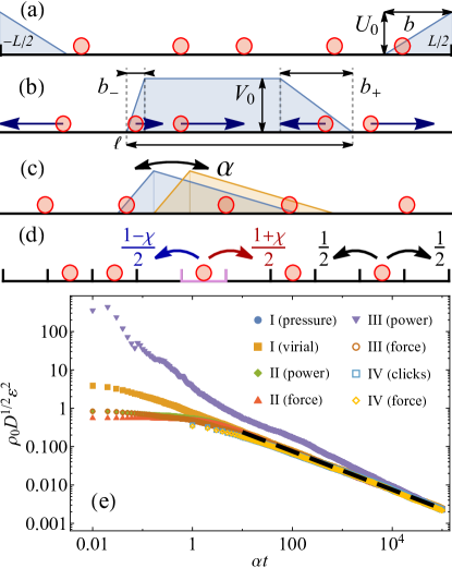
Figure 2: (a-d) Sketches of Models 2-2 (respectively). (e) The squared relative uncertainty of the time-averaged steady-state pressure $\mathscr{P}(t)$, virial $\mathcal{V}(t)$ (2), exerted force $F(t)$ (2-2), consumed power $\mathcal{P}(t)$ (2-2) and detector clicks $C(t)$ (2); simulations (colored symbols) and the universal asymptotic prediction Eq. (1) (black dashed line). Pressure and virial symbols overlap. Parameters: $\rho_{0}\!=\!v=\!\mu\!=\!\alpha\!=\!T\!=\!1$, $L=10^{4}$. 2: $U_{0}=30$, $b=3$. 2-2 (respectively): $V_{0}\!=\!0.25,7.5$, $b_{-}\!=\!0.26,1.25$, $b_{+}\!=\!0.74,8.75$, $\ell\!=\!1,5$. 2: $\chi\!=\!0.5$.

Equation (1) is demonstrated numerically in Fig. 2 for $d=1$ – the integer dimension for which the anomalous effect is most pronounced – and for four distinct probe models detailed below (see Fig. 2(a-d)): (I) Brownian particles in a soft box, (II) active run-and-tumble particles interacting with a localized asymmetric obstacle [21, 22, 68, 41], (III) a localized variant of the Ajdari-Prost model [69, 70, 71] for Brownian particles driven by stochastic ratchet potentials and (IV) random walkers on a lattice, driven by a pointlike pump [7].

Two observables are measured for each model. For the equilibrium Model 2, these are the net pressure $\mathscr{P}(t)$ exerted on the box walls and the Clausius virial $\mathcal{V}(t)$, defined explicitly below. Both are thermodynamic observables that admit the ideal-gas equations of state $\langle\mathscr{P}\rangle\!=\!\rho_{0}T$ and $\langle\mathcal{V}\rangle\!=-\!\rho_{0}LT/2$ respectively. For the nonequilibrium Models 2-2, the observables are the net force $F(t)$ the probe exerts and the rate $\mathcal{P}(t)$ of total work performed on the particles (consumed power). The latter satisfies $\langle\mathcal{P}\rangle\!\neq\!0$ only out of equilibrium. For Model 2, $F(t)$ and the clicks $C(t)$ in a particle detector are measured. In Fig. 2(e), the squared relative uncertainties of all eight observables are shown to collapse on the curve predicted by Eq. (1) in the long-time limit. The simulation details are provided below, followed by a systematic derivation of Eq. (1). Implications and extensions are then discussed.

Simulation details.— Model 2 is given by

$$\dot{x}_{n}(t) =-\mu U^{\prime}\left[x_{n}(t)\right]+\sqrt{2\mu T}\eta_{n}(t)\;.$$ (3)

Here, $\{x_{n}(t)\}_{n=1}^{N}$ are the particle positions, $\mu$ is the mobility and the potential $U(x)$ describes the interaction with soft walls of width $b$ and potential height $U_{0}$ (see Fig. 2(a)). The mass diffusivity is given by the Einstein relation $D=\mu T$. Periodic boundary conditions are implemented, and $U_{0}/T$ is set sufficiently high such that the typical crossing time is much longer than the simulation duration [72]. The walls are then effectively impenetrable. Regardless, the wall penetrability does not affect the equations of state and the validity of the results.

Model 2 is given by the continuous-time stochastic equations of motion

$$\dot{x}_{n}(t) =vu_{n}(t)-\mu V^{\prime}\left[x_{n}(t)\right]\;.$$ (4)

Here, the potential $V(x)$ describes the interaction with a penetrable asymmetric obstacle of total length $\ell$, potential height $V_{0}$ and left and right side widths $b_{-}$ and $b_{+}$ respectively, (see Fig. 2(b)) . The particles are propelled by the active force $vu_{n}(t)/\mu$, where $v$ is the propulsion speed and $u_{n}(t)=\pm 1$ is a telegraphic internal degree of freedom. The latter flips at a Poissonian rate $\alpha/2$, such that $\langle u_{m}(t)u_{n}(t^{\prime})\rangle_{c}=\delta_{mn}e^{-\alpha|t-t^{\prime}|}$.

Model 2 is given by the Itô-Langevin equations

$$\dot{x}_{n}(t) =-\mu V^{\prime}\left[x_{n}(t)+b_{-}w_{n}(t)\right]+\sqrt{2\mu T}\eta_{n}(t)\;,$$ (5)

where $T$ is the ambient temperature, $\eta_{n}(t)$ is a Gaussian white noise of unit variance, $w_{n}(t)\!\equiv\!\left[1+u_{n}(t)\right]/2$ and $u_{n}(t)$ are as defined above. Both Models 2-2 incorporate driving via the persistent noise $u_{n}(t)$, a fast variable that relaxes to its steady state over a finite timescale $\alpha^{-1}$. For $t\gg\alpha^{-1}$, the dynamics become diffusive with effective diffusivities $D=v^{2}/\alpha$ (Model 2) and $D=\mu T$ (Model 2). Models 2-2 were all simulated in a periodic system $\left[-L/2,L/2\right]$ where $L\gg v/\alpha,\ell$.

Lastly, in Model 2, particles perform discrete-time random walks on a one-dimensional periodic lattice of $L\gg 1$ sites. A particle at site $x$ at time $t$ hops at time $t+1$ to $x\pm 1$ with probability $1/2$. A bias $\chi$ is introduced at $x=0$, such that the probability of hopping to $x=\pm 1$ is $(1\pm\chi)/2$. The particle is thus driven by a localized non-conservative force $f(0\!\leftrightarrow\!\pm 1)\!=\!\pm\ln(1\pm\chi)/2$ and $f(x\!\leftrightarrow\!x^{\prime})\!=\!0$ for any other bond $x\!\leftrightarrow\!x^{\prime}$ [72]. Its macroscopic dynamics are diffusive with $D\!=\!1/2$ and $f(x)\!\simeq\!\chi\delta(x)$.

To obtain Fig. 2, the net force exerted by the probe is measured as $F(t)\!=\!\sum_{n}f_{n}(t)$, where

$$f_{n}(t)=\begin{dcases}-U^{\prime}[x_{n}(t)]\;,&\rm{Model\;\ref{word:I}}\\ -V^{\prime}[x_{n}(t)]\;,&\rm{Model\;\ref{word:II}}\\ -V^{\prime}[x_{n}(t)+b_{-}w_{n}(t)]\;,&\rm{Model\;\ref{word:III}}\\ f[x_{n}(t+1)\leftrightarrow x_{n}(t)]\;,&\rm{Model\;\ref{word:IV}}\end{dcases}.$$ (6)

The rate of total work performed on the particles is measured as the residual power $\mathcal{P}(t)$ dissipated due to the introduction of the probe. It is given by $\mathcal{P}(t)\!=\!\sum_{n}\left[\dot{x}_{n}F_{n}(t)\!-\!\dot{x}_{n}F_{n}(t)|_{f_{n}(t)=0}\right]$, where $F_{n}(t)$ is the net athermal force exerted on the particle. For, Models 2-2, the definition becomes

$$\mathcal{P}(t)=\sum_{n}\begin{dcases}\left[\dot{x}_{n}(t)+vu_{n}(t)\right]f_{n}(t)\;,&\rm{Model\;\ref{word:II}}\\ \dot{x}_{n}(t)\circ f_{n}(t)\;,&\rm{Model\;\ref{word:III}}\end{dcases},$$ (7)

where $\circ$ is the Stratonovich product. The clicks $C(t)$ in a detector at $x=0$ are given by $C(t)\!=\!\sum_{n}\delta_{x_{n}(t),0}$ . The pressure $\mathscr{P}(t)$ is measured as the net normal force on the two walls, i.e. $\mathscr{P}(t)\!=-\!\sum_{n}\!{\rm sgn}(x_{n}(t))f_{n}(t)/2$. Lastly, the Clausius virial is defined as $\mathcal{V}(t)\!=-\!\sum_{n}x_{n}(t)f_{n}(t)/2$.

Theory.—The derivation of Eq. (1) relies on the long-time tail of the single-particle propagator $P(\mathbf{y},t|\mathbf{y}^{\prime},0)$. Here, the generalized particle coordinate $\mathbf{y}=(\mathbf{r},\mathbf{u})$ includes both its position $\mathbf{r}$ in a $d$-dimensional space of size $L\rightarrow\infty$ and any internal degrees of freedom $\mathbf{u}$, such as the telegraphic ones in Models 2-2. It is shown below that the propagator long-time tail is given, to leading order, by 

$$P(\mathbf{y},t|\mathbf{y}^{\prime},0) =\frac{\rho_{\text{s}}(\mathbf{y})}{\rho_{0}}\left(4\pi Dt\right)^{-d/2}+\mathcal{O}(t^{-(d/2+1)})\;,$$ (8)

where $\rho_{\text{s}}(\mathbf{y})$ is the nonequilibrium steady-state density, which satisfies $\lim_{r\rightarrow\infty}\int d\mathbf{u}\rho_{\rm s}(\mathbf{r},\mathbf{u})\!=\!\rho_{0}$.

Equation (8) reveals that the leading order long-time tail is independent of the initial conditions . It generalizes previous results for one-dimensional Brownian [77, 46, 78] and run-and-tumble particles [41]. Heuristically, at late times, $P(\mathbf{y},t|\mathbf{y}^{\prime},0)$ is dominated by trajectories of particles that avoid long excursions and remain near $\mathbf{y}$. Such particles forget their initial coordinate $\mathbf{y}^{\prime}$ and relax to a local steady state, i.e. $P(\mathbf{y},t|\mathbf{y}^{\prime},0)\sim\rho_{\rm s}(\mathbf{y})$ up to a normalization factor. Since the probability density $P(\mathbf{y},t|\mathbf{y}^{\prime},0)$ expands diffusively at late times, it is supported on a large region of volume $\sim(Dt)^{d/2}$. This implies a normalization factor $\sim 1/\rho_{0}(Dt)^{d/2}$.

Equation (8) can be applied to obtain the long-time tails of two-time correlation functions of arbitrary stationary and local observables $A(t)=\sum_{n}a(\mathbf{y}_{n}(t))$ and $B(t)=\sum_{n}b(\mathbf{y}_{n}(t))$, where $\{\mathbf{y}_{n}\!=\!(\mathbf{r}_{n},\mathbf{u}_{n})\}_{n=1}^{N}$ are the generalized coordinates of all particles. Here, local means that $a(\mathbf{y})$ and $b(\mathbf{y})$ vanish rapidly when $r=|\mathbf{r}|$ exceeds some finite range, meaning that the probe is centered at $\mathbf{r}=0$. For $N=\rho_{0}L^{d}$ non-interacting particles, the correlation $\langle A(t)B(0)\rangle_{c}=\langle A(t)B(0)\rangle{-}\langle A\rangle\langle B\rangle$ is given by $N\langle a\left(\mathbf{y}_{1}(t)\right)b\left(\mathbf{y}_{1}(0)\right)\rangle_{c}$. Since $\langle a\rangle=\langle A\rangle/N$, $\langle A(t)B(0)\rangle_{c}$ can be expressed explicitly as

$$\left\langle A(t)B(0)\right\rangle_{c} \!=\!\int\!d\mathbf{y}d\mathbf{y}^{\prime}\!a(\mathbf{y})P(\mathbf{y},t|\mathbf{y}^{\prime},0)b(\mathbf{y}^{\prime})\rho_{\text{s}}(\mathbf{y}^{\prime}),$$ (9)

with an $\mathcal{O}(N^{-1})=\mathcal{O}(L^{-d})$ correction for finite systems. Inserting Eq. (8) and $\langle A\rangle\!=\!\int d\mathbf{y}\rho_{\rm s}(\mathbf{y})a(\mathbf{y})$ then leads to

$$\left\langle A(t)B(0)\right\rangle_{c} =\frac{\left\langle A\right\rangle\!\left\langle B\right\rangle}{\rho_{0}}\left(4\pi Dt\right)^{-d/2}\!+\!\mathcal{O}(t^{-(d/2+1)}).$$ (10)

Due to time-translation invariance,

$$\left\langle\bar{A}^{2}(t)\right\rangle_{c}=\frac{2}{t^{2}}\int_{0}^{t}dt_{1}\int_{0}^{t_{1}}dt_{2}\left\langle A(t_{1})A(t_{2})\right\rangle_{c}\;.$$ (11)

Inserting Eq. (10) into Eq. (11) with $B(t)=A(t)$ then leads to

$$\left\langle\bar{A}^{2}(t)\right\rangle_{c}\sim\!\begin{dcases}\frac{8\left\langle A\right\rangle^{2}}{\rho_{0}\!\left(8\!-\!6d\!+\!d^{2}\right)\!(4\pi D)^{\frac{d}{2}}}t^{-\frac{d}{2}},\!&\!d<2\\ \frac{\left\langle A\right\rangle^{2}}{2\pi D\rho_{0}}\frac{\ln t}{t},\!&\!d=2\\ \!2\mathcal{D}_{A}t^{-1},\!&\!d>2\end{dcases}.$$ (12)

Equation (1) then follows from Eq. (12) and $\langle\bar{A}(t)\rangle=\langle A\rangle$. For $d\leq 2$, the fluctuations are superdiffusive, i.e. $\langle\bar{A}^{2}(t)\rangle_{c}$ decays slower than $\sim t^{-1}$. This shift originates in the nonintegrability of $\langle A(t)A(0)\rangle_{c}\sim t^{-d/2}$ for $d\leq 2$ and relies on $\langle A\rangle\neq 0$. If $\langle A\rangle=0$, the leading-order tail in Eq. (10) shifts from $\sim t^{-d/2}$ to $\sim t^{-(d/2+1)}$. The latter is integrable for any $d$, implying normal diffusion.

Derivation of Eq. (8).—The derivation follows the eigenstate expansion approach devised for a one-dimensional Brownian particle [46, 78]. Here, the derivation applies to a generic continuous-time Markov process with long-time diffusive behavior. Its dynamics are specified by the master equation

$$\frac{d}{dt}\left|P(t)\right\rangle =M\left|P(t)\right\rangle,$$ (13)

where $M$ is a Markov generator and $\langle\mathbf{y}|P(t)\rangle$ specifies the probability density at $\mathbf{y}$. The single-particle steady-state distribution $P_{\rm{s}}(\mathbf{y})=\langle\mathbf{y}|0\rangle$ is related to the steady-state density $\rho_{\rm{s}}(\mathbf{y})$ via $\rho_{\rm{s}}(\mathbf{y})=NP_{\rm{s}}(\mathbf{y})$. The solution to Eq. (13) is

$$\left|P(t)\right\rangle =U(t)\left|P(0)\right\rangle,$$ (14)

where $U(t)=e^{tM}$ is the time-evolution operator. Using the right eigenvectors $|n\rangle$, left eigenvectors $\langle n|$ and eigenvalues $\epsilon_{n}$, it can be spectrally decomposed as

$$U(t) =\sum_{n=0}^{\infty}e^{-\epsilon_{n}t}\left|n\right\rangle\left\langle n\right|.$$ (15)

Due to the Markov property of $M$, it holds that $\epsilon_{0}=0$ and ${\rm Re}\,\epsilon_{n}\geq{\rm Re}\,\epsilon_{n-1}$ for any $n>0$. Therefore, the contributions to Eq. (15) due to $|n\rangle\langle n|$, $n\gg 1$, become exponentially suppressed in the long-time limit. In this limit, it is thus sufficient to truncate the expansion at the small-$\epsilon_{n}$ part of the spectrum.

To this end, it is first assumed that the effective dynamics are diffusive on large scales, i.e., sufficiently far away from the origin, for every solution $|P(t)\rangle$,

$$\left\langle\mathbf{r}\left|M\right|P\right\rangle =D_{ij}\partial_{i}\partial_{j}\left\langle\mathbf{r}|P\right\rangle+\mathcal{O}\!\left[\partial_{\mathbf{r}}^{3}\left\langle\mathbf{r}|P\right\rangle\right],$$ (16)

where $\langle\mathbf{r}|\equiv\int d\mathbf{u}\langle\mathbf{y}|$, $\partial_{i}\equiv\partial_{r_{i}}$ and $D_{ij}$ is the effective macroscopic diffusivity tensor. Without loss of generality, the latter is taken to be isotropic, i.e. $D_{ij}=D\delta_{ij}$ where $\delta_{ij}$ is the Kronecker delta. The general anisotropic case can be mapped to the isotropic one by diagonalization and rescaling of the principal axes. Equation (16) implies that, in the limit $L\rightarrow\infty$, the lowest excited states are diffusive modes, whose spatial contribution to the spectral gap vanishes in this limit . These states satisfy the standard plane-wave scattering form [80]

$$\left\langle\mathbf{r}|n\right\rangle\sim \frac{1}{L^{d}}\left[e^{-i\mathbf{q}\cdot\mathbf{r}}+f(\hat{\mathbf{q}},\hat{\mathbf{r}})\frac{e^{iqr}}{r^{(d-1)/2}}\right]\;,\quad r\rightarrow\infty\;,$$ (17)

where $\mathbf{q}$ solves $\epsilon_{n}=Dq^{2}$, $\hat{\mathbf{r}}\equiv\mathbf{r}/r$ and $f(\hat{\mathbf{q}},\hat{\mathbf{r}})$ is the scattering amplitude, whose particular structure is unimportant to the derivation.

The second assumption is timescale separation: it is assumed that $\mathbf{u}(t)$ is a fast stochastic variable that relaxes at a characteristic rate $\alpha>0$ such that adiabatic elimination is applicable. The latter shows that, for $t\gg\alpha^{-1}$, any solution $|P(t)\rangle$ satisfies [81, 82]

$$\langle\mathbf{y}\left|P(t)\right\rangle \simeq W\left[\langle\mathbf{r}\left|P(t)\right\rangle\right](\mathbf{y})\;,$$ (18)

where $W$ is an operator determined by $M$. For example, when $\mathbf{u}$ and $\mathbf{r}$ are decoupled, $W[g(\mathbf{r})](\mathbf{y})=P_{\rm s}(\mathbf{u})g(\mathbf{r})$, where $P_{\rm s}(\mathbf{u})=\int d\mathbf{r}P_{\rm s}(\mathbf{y})$. Note that Eq. (18) is equivalent to $|P(t)\rangle\simeq W\Pi|P(t)\rangle$, where $\Pi=\int d\mathbf{r}|\mathbf{r}\rangle\langle\mathbf{r}|$ is a projection operator. Applying Eq. (18) to the solutions $|P(t)\rangle=e^{-\epsilon_{n}t}|n\rangle$ provides that the lowest excited state $|n\rangle$ with a given projection $\langle\mathbf{r}|n\rangle$ is $\langle\mathbf{y}|n\rangle=W\left[\langle\mathbf{r}|n\rangle\right](\mathbf{y})$ such that $\epsilon_{n}\ll\alpha$. In combination with Eq. (17), this allows to index the lowest excited states by $\mathbf{q}$, i.e. define $|\mathbf{q}\rangle\equiv L^{d}|n\rangle$ and $\langle\mathbf{q}|\equiv\!\langle n|$. The ground state is then $|\mathbf{q}=0\rangle=L^{d}|n=0\rangle$.

In the long-time limit, only the first terms in Eq. (15) corresponding to the diffusive soft modes $|\mathbf{q}\rangle$ contribute, leaving

$$U(t) \sim\frac{1}{L^{d}}\sum_{\mathbf{q}}e^{-\epsilon(\mathbf{q})t}\left|\mathbf{q}\right\rangle\left\langle\mathbf{q}\right|\;,$$ (19)

where $\epsilon(\mathbf{q})=Dq^{2}$. In the limit $L\rightarrow\infty$, the sum converges to the integral

$$U(t) \sim\int\frac{d^{d}\mathbf{q}}{(2\pi)^{d}}e^{-\epsilon(\mathbf{q})t}\left|\mathbf{q}\right\rangle\left\langle\mathbf{q}\right|\;.$$ (20)

The last step is a saddle-point approximation of Eq. (20) in the limit $t\rightarrow\infty$, which amounts to expanding $|\mathbf{q}\rangle$ as $|\mathbf{q}\rangle=|0\rangle+\mathcal{O}(q)$ and evaluating the Gaussian integral. The result is

$$U(t) =\left|0\right\rangle\left\langle 0\right|\left(4\pi Dt\right)^{-d/2}+\mathcal{O}(t^{-(d/2+1)})\;.$$ (21)

In the basis $\{|\mathbf{y}\rangle\}$, it holds that $P(\mathbf{y},t|\mathbf{y}^{\prime},0)\!\equiv\!\langle\mathbf{y}|U(t)|\mathbf{y}^{\prime}\rangle$, $\langle 0|\mathbf{y}^{\prime}\rangle\!=\!1$ and $\langle\mathbf{y}|0\rangle\!=\!L^{d}P_{\text{s}}(\mathbf{y})$. The factor of $L^{d}$ stems from the redefinition of $|0\rangle$ in Eq. (19). Using $\rho_{\rm{s}}(\mathbf{y})\!=\!\rho_{0}L^{d}P_{\rm{s}}(\mathbf{y})$ then leads to Eq. (8).

Discussion.—In this Letter, the anomalous power law Eq. (1) was found for local probe measurements in $d\leq 2$ systems. The anomalous scaling stems from the recurrence property of random walks for $d\leq 2$ [83, 84, 85, 86]. Here, it is manifested through the nonintegrability of $P(\mathbf{y},t|\mathbf{y}^{\prime},0)\sim t^{-d/2}$, as seen from Eq. (8). The prefactors were found to be universal: they are insensitive to microscopic details and depend solely on the macroscopic properties $\rho_{0}$ and $D$.

The results presented here can be generalized in several ways. First, since Eq. (10) provides the long-time tails for both autocorrelations and cross-correlations, Eq. (1) can be immediately generalized to

$$\varepsilon_{AB}^{2}(t)\!\sim\! \begin{dcases}\!8\rho_{0}^{-1}\!\left(8\!-\!6d\!+\!d^{2}\right)^{-1}\!(4\pi Dt)^{-d/2},\!&\!d<1\\ \!\rho_{0}^{-1}(2\pi Dt)^{-1}\ln t,\!&\!d=2\\ \!2\mathcal{D}_{AB}\left\langle A\right\rangle^{-1}\left\langle B\right\rangle^{-1}t^{-1},\!&\!d>2\end{dcases},$$ (22)

where $\varepsilon_{AB}^{2}(t)\!\equiv\!\langle\bar{A}(t)\bar{B}(t)\rangle_{\rm c}/\langle\bar{A}\rangle\langle\bar{B}\rangle$, $\mathcal{D}_{AB}\!\equiv\!\int_{0}^{\infty}dtC_{AB}(t)$ and $2C_{AB}(t)\!\equiv\!\langle A(t)B(0)\rangle_{c}\!+\!\langle B(t)A(0)\rangle_{c}$.

Second, the timescale separation assumption used in the derivation of Eq. (8) applies to a broad class of fast variables, such as spatial degrees of freedom below a given microscopic scale. Hence, the results can be extended to heterogeneous systems with, e.g. disordered or periodic potentials of vanishing mean, for which the effective diffusivity depends on the microscopic structure [87, 88, 89, 90, 91, 92].

Lastly, internal noise in the measurement, independent of the particle positions, can be introduced via the fast degrees of freedom $\{\mathbf{u}_{n}\}$. Extending the results to dynamical probes (e.g. tracer particles [93]) is expected to rely on adiabatic expansion methods [94, 95, 96, 41, 97].

Whether the universality extends to dense systems, for which interactions cannot be neglected, remains an open question. Since the derivation here relies solely on the effective macroscopic dynamics, it is expected that if the latter remains diffusive, the results generalize directly with $D$ getting dressed by the interactions.