Impact of Charge on Traversable Wormhole Solutions in f(R,T) Theory

Abstract

This paper examines the effects of charge on traversable wormhole structure in $f(R,T)$ theory. For this purpose, we use the embedding class-I approach to build a wormhole shape function from the static spherically symmetric spacetime. The developed shape function satisfies all the required conditions and connects two asymptotically flat regions of spacetime. We consider different models of this modified theory to examine the traversable wormhole solutions through null energy condition and also check their stable state. We conclude that viable and stable wormhole solutions are obtained under the influence of charge in this gravitational theory.

Keywords: Wormhole solutions; Electromagnetic field; $f(R,T)$ theory; Karmarkar condition.
PACS: 04.50.Kd; 03.50.De; 98.80.Cq; 04.40.Nr.

1 Introduction

Different cosmic observations such as supernovae type 1a, the large-scale structures and the cosmic microwave background radiations reveal that our universe is in accelerated expansion phase [1]. Researchers claim that this expansion is the result of some mysterious force known as dark energy. The lambda cold dark matter model based on general relativity (GR) is the first model which provides a mathematical framework for understanding the effects of dark energy on the spacetime. However, this model has fine-tuning and coincidence problems. Different modified theories have been developed to resolve these issues. The $f(R)$ gravity is the first and simplest modification which is obtained by incorporating the Ricci scalar $(R)$ with its generic function in the Einstein-Hilbert action. The important literature is available for understanding various characteristics of this modified theory [2]-[5]. Harko et al [6] introduced $f(R,T)$ theory by incorporating the trace of energy-momentum tensor (EMT) in the functional action of $f(R)$ gravity. This is one of the modified theories that has been established to study the impact of curvature-matter interaction on cosmic structures [7]-[16]. Sharif and Waseem [17] used the Krori-Barua solutions and examined the viability of anisotropic quark stars in this theory.

The study of hypothetical structures in the universe such as wormhole (WH) is a fascinating area of research. The term WH refers to a non-singular solution of the field equations that creates a shortcut among two distinct areas of the universe. Wormholes are thought to be formed by a process called “gravitational collapse”. This occurs when a massive object collapses due to the force of gravity. The resulting spacetime distortion may create a bridge or WH between two distant points in the universe. An intra-universe WH connects two distant points within the same universe and an inter-universe WH connects two different universes. Flamm [18] was the first who constructed the isometric embedding of the Schwarzschild solution, which is considered to be an early precursor to the concept of WHs. Later, Einstein and Rosen [19] investigated that the spacetime can be connected by a tunnel-like structure, allowing for a shortcut or bridge between two distant regions of spacetime, called Einstein-Rosen bridge. Wheeler [20] showed that Schwarzschild WH solutions are non-traversable because the throat of the WH can change its size and shape. Ellis [21] invented the term “Drainhole” to describe a WH.

In 1988, Morris and Thorne [22] published a paper in which they proposed the concept of a traversable WH. A WH is “traversable” if it allows the matter to travel without getting destroyed by the extreme gravitational forces present inside it. They proposed that a WH can be traversable if it is stabilized by a form of exotic matter with negative energy density. This exotic matter would need to have specific properties such as negative pressure to counteract the gravitational pull otherwise causes the WH to collapse. Exotic matter can be used to control the size and shape of the WH throat, preventing it from closing off too quickly. One proposal for confining exotic matter in the interior space of WH is through the use of “matching conditions” [23]. These conditions are mathematical equations that define how the geometry of one region of a WH match with the geometry of another region for traversable and stable WH structure. Spherical traversable WHs are most commonly studied and can only exist in the presence of exotic matter [24]. Additionally, phantom energy has been used to construct static spherical WHs [25, 26]. It is believed that cylindrical WHs may be able to exist under slightly different conditions as compared to spherically symmetric WHs [27]-[29]. Gibbons and Volkov [30] discussed how Einstein-Rosen and Flamm’s solutions relate to each other.

Shape functions are important in determining the properties and behavior of traversable WHs. It is a mathematical function that describes the spatial geometry of the WH, specifically the radius of throat as a function of the radial coordinate. Different shape functions can be used to model different types of WHs. For example, the Morris-Thorne shape function is commonly used to model WHs with spherical symmetry [31]. The choice of shape function can greatly affect the properties of WH such as stability, traversability and the required amount of exotic matter to keep the WH throat open. Sharif and Fatima [32] used two different shape functions to investigate the viability of non-static conformal WHs. Cataldo et al [33] studied static traversable WH solutions by constructing a shape function that connects two asymptotically non-flat regions of spacetime. In the framework of $f(R)$ gravity, Godani and Samanta [34] used two different shape functions and introduced new WH structures. Sharif and Gul [35] used Noether symmetry technique to check the viability and stability of WH geometry corresponding to different redshift and shape functions in $f(R,T^{2})$ theory, where $T^{2}$ is the self-contraction of EMT.

The effect of electric charge can significantly impact the geometry and stability of WHs. In particular, the electric charge can create a repulsive force that pushes the walls of WH apart making the throat of WH wider. This can affect the stability of WH as it may require a greater amount of energy to keep the throat open. There has been several works exploring the influence of charge on the structure of WH. Reissner and Nordstr$\ddot{o}$m presented the first static charged solution of the Einstein-Maxwell field equations, which describe the gravitational and electromagnetic fields in GR. Esculpi and Aloma [36] studied the impact of anisotropy on charged compact objects by using a linear equation of state. Sharif and Mumtaz constructed charged thin-shell WHs using Visser cut and paste approach [37]. Moraes et al [38] constructed charged WHs in the context of curvature matter coupled gravity. Sharif and Naz [39] studied the dynamics of charged cylindrical collapse in $f(G)$ theory ($G$ is the Gauss-Bonnet invariant) and found that Gauss-Bonnet terms and charge prevent gravitational collapse. Sharif and Javed [40] used the cut and paste approach to examine the influence of charge and Weyl coupling parameters on thin-shell WHs.

The scientific community has shown great interest in studying the WH structures in modified theories. Elizalde and Khurshudyan [41] used the barotropic equation of state to examine the viability and stability of WH geometry in curvature-matter coupled gravity. Sharif and Shahid [42] used the Noether symmetry technique to study the WH solutions with isotropic matter configuration in $f(G,T)$ gravity. Shamir and Fayyaz [43] built a WH shape function using Karmarkar condition in the modified $f(R)$ theory. In the same theory, Mishra et al [44] found traversable WH solutions using three different models of $f(R)$ gravity. Shamir et al [45] analyzed WH solutions with anisotropic matter configuration in $f(R)$ gravity. Recently, we have employed the Karmarkar condition and investigated the viable WH structure with anisotropic matter configuration in $f(R,T)$ theory [46].

This paper analyzes the impact of charge on traversable WH solutions using the Karmarkar condition in $f(R,T)$ theory. We have arranged the paper as follows. We construct the shape function admitting Karmarkar condition in section 2. In section 3, we use charged anisotropic matter configuration to construct the field equations and examine the nature of null energy condition by considering two different models of this gravity. The stable state of the resulting WH solutions is checked in section 4. In the last section we compile our obtained results.

2 Karmarkar Condition

Here, we employ the Karmarkar condition to develop the WH shape function which describes the WH geometry. In this perspective, we assume static spherically symmetric spacetime as

$$ds^{2}=e^{\lambda(r)}dt^{2}-e^{\psi(r)}dr^{2}-r^{2}(d\theta^{2}+\sin^{2}\theta d\phi^{2}).$$ (1)

The non-zero components of the curvature tensor for the above spacetime are given as

$$R_{1212} = \frac{e^{\lambda}(2\lambda^{\prime\prime}+\lambda^{\prime 2}-\lambda^{\prime}\psi^{\prime})}{4},\quad R_{3434}=\frac{r^{2}\sin^{2}\theta(e^{\psi}-1)}{e^{\psi}},$$

$$R_{1414} = \frac{r\sin^{2}\theta\lambda^{\prime}e^{\lambda-\psi}}{2},\quad R_{2323}=\frac{r\psi^{\prime}}{2},\quad R_{1334}=R_{1224}\sin^{2}\theta,$$

where $R_{1224}=0$. These components fulfill the well-known Karmarkar condition as

$$R_{1414} = \frac{R_{1212}R_{3434}+R_{1224}R_{1334}}{R_{2323}},\quad R_{2323}\neq 0.$$ (2)

Embedding class-I is the type of spacetime that fulfills the Karmarkar condition. By substituting the values of non-zero Riemann components in the Karmarkar condition, we get

$$\frac{\lambda^{\prime}\psi^{\prime}}{1-e^{\psi}}=\lambda^{\prime}\psi^{\prime}-2\lambda^{\prime\prime}-\lambda^{\prime 2},\quad e^{\psi}\neq 1.$$

We solve the above equation and obtain the solution as

$$e^{\psi}=1+Ce^{\lambda}\lambda^{\prime 2},$$ (3)

here $C$ is an arbitrary constant.

In order to construct the WH shape function, we take the Morris-Thorne metric as

$$ds^{2}=e^{\lambda(r)}dt^{2}-\frac{1}{1-\frac{d(r)}{r}}dr^{2}-r^{2}d\theta^{2}-r^{2}\sin\theta d\phi^{2}.$$ (4)

Here, $d(r)$ is the shape function and $\lambda(r)$ is the redshift function which is defined as $\lambda(r)=\frac{-2\epsilon}{r}$, where $\epsilon$ is an arbitrary constant and, when $r\rightarrow\infty$, $\lambda(r)\rightarrow 0$ [47]. From Eqs.(1) and (4), we have

$$\psi(r)=\ln\bigg{[}\frac{r}{r-d(r)}\bigg{]}.$$ (5)

We use Eqs.(3) and (5) to get the shape function as

$$d(r)=r-\frac{r^{5}}{r^{4}+4\epsilon^{2}Ce^{\frac{-2\epsilon}{r}}}.$$ (6)

The following conditions of shape function must be satisfied for a viable WH structure [22].

1. $d(r)<r$,

2. $d(r)-r=0$ at $r=b$,

3. $\frac{d(r)-rd^{\prime}(r)}{d^{2}(r)}>0$ at $r=b$,

4. $d^{\prime}(r)<1$,

5. The condition $\frac{d(r)}{r}\rightarrow 0$ should be satisfied when $r\rightarrow\infty$,

where $b$ is known as WH throat radius. At WH throat, Eq.(6) gives a trivial solution such that $d(b)-b=0$ at $b=0$. We add a free parameter $(A)$ in Eq.(6) to get a non-trivial solution as

$$d(r)=r-\frac{r^{5}}{r^{4}+4\epsilon^{2}Ce^{\frac{-2\epsilon}{r}}}+A.$$ (7)

For a viable WH geometry, these conditions must be fulfilled. These conditions are satisfied for $0<A<b$, otherwise the required conditions are not satisfied and one cannot obtain the viable WH structure. By using condition 2 in the above equation, we get $C=\frac{b^{4}(b-A)}{4b\epsilon^{2}e^{\frac{-2\epsilon^{2}}{b}}}$. Inserting this value in Eq.(7), we get the shape function as

$$d(r)=r-\frac{r^{5}}{r^{4}+b^{4}(\frac{b}{A}-1)}+A.$$ (8)

We can see that our developed shape function also satisfies the other conditions and hence asymptotically flat traversable WH geometry is obtained. For our convenience, we assume $b=2$ and $\epsilon=-1$ to analyze the graphical nature of the WH shape function. Figure 1 indicates that for different values of $A$, all conditions meet the required criteria. The values of $A=1.9,1.8,1.7,1.6$ represent black, green, red and yellow colors, respectively.

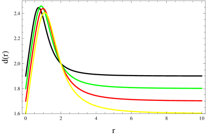
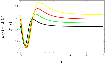
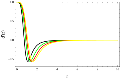
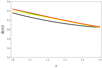
Figure 1: Plots of shape function conditions with respect to radial coordinate.

3 $f(R,T)$ Gravity

The integral action for $f(R,T)$ theory is given as [48]

$$I=\int dx^{4}\sqrt{-g}\bigg{[}\frac{f(R,T)}{2k}+L_{m}+L_{e}\bigg{]},$$ (9)

where $L_{m}$ is the matter-Lagrangian, $g$ is the determinant of the metric tensor and $L_{e}=sF_{\chi\eta}F^{\chi\eta}$, where $s$ is an arbitrary constant. Here $F_{\chi\eta}=\phi_{\eta,\chi}-\phi_{\chi,\eta}$ is the electromagnetic field tensor and $\phi_{\chi}$ is the four potential. The corresponding field equations are

$$R_{\chi\eta}f_{R}-\frac{1}{2}g_{\chi\eta}f-(\nabla_{\chi}\nabla_{\eta}-g_{\chi\eta}\Box)f_{{}_{R}}+f_{T}\Theta_{\chi\eta}+f_{T}T_{\chi\eta}=T_{\chi\eta}+E_{\chi\eta}.$$ (10)

Here, $f_{R}=\frac{\partial f}{\partial R}$ and $f_{T}=\frac{\partial f}{\partial T}$. The equation of $\Theta_{\chi\eta}$ is given as

$$\Theta_{\chi\eta}=-2T_{\chi\eta}+g_{\chi\eta}L_{m}-2g^{\varpi\sigma}\frac{\partial^{2}L_{m}}{\partial g^{\chi\eta}\partial g^{\varpi\sigma}},$$ (11)

and EMT of electric field is expressed as

$$E_{\chi\eta}=\frac{1}{4\pi}\bigg{(}\frac{F^{\varpi\sigma}F_{\varpi\sigma}g_{\chi\eta}}{4}-F^{\varpi}_{\chi}F_{\eta\varpi}\bigg{)}.$$ (12)

We assume that the WH interior geometry is filled with anisotropic fluid, given as

$$T_{\chi\eta}=(P_{r}-P_{t})U_{\chi}U_{\eta}-P_{t}g_{\chi\eta}+(\rho+P_{t})V_{\chi}V_{\eta},$$ (13)

where $\rho$ represents the energy density, $V_{\chi}$ is the four-velocity, $U_{\chi}$ defines four-vector, $P_{r}$, $P_{t}$ are radial and tangential pressure, respectively. We consider $L_{m}=-\frac{1}{4}F_{\chi\eta}F^{\chi\eta}$ which leads to $\frac{\partial^{2}L_{m}}{\partial g^{\chi\eta}\partial g^{\varpi\sigma}}=-\frac{1}{2}F_{\chi\varpi}F_{\eta\sigma}$ [49]. Thus, Eq.(11) becomes

$$\Theta_{\chi\eta}=-2T_{\chi\eta}+g_{\chi\eta}L_{m}+2g^{\varpi\sigma}F_{\chi\varpi}F_{\eta\sigma}.$$

We can rewrite Eq.(10) as

$$G_{\chi\eta}=\frac{1}{f_{R}}[T_{\chi\eta}+E_{\chi\eta}+T^{d}_{\chi\eta}],$$ (14)

where $T^{d}_{\chi\eta}$ are the additional effects of $f(R,T)$ theory named as dark source terms, expressed as

$$T^{d}_{\chi\eta}=\bigg{[}\frac{1}{2}(f-Rf_{R})g_{\chi\eta}-(g_{\chi\eta}\Box-\nabla_{\chi}\nabla_{\eta})f_{R}-(T_{\chi\eta}+\Theta_{\chi\eta})f_{T}\bigg{]}.$$ (15)

The Maxwell field equations are defined as

$$F_{\chi\eta;\varpi}=0,\quad F^{\chi\eta}_{;\sigma}=4\pi J^{\chi},$$ (16)

where $J^{\chi}$ is defined as four current. In comoving coordinates, both $\phi^{\chi}$ and $J^{\chi}$ fulfill the following relations

$$\phi^{\chi}=\phi(r)\delta^{\chi}_{0},\quad J^{\chi}=\varrho(r)V^{\chi},$$ (17)

where $\varrho$ is the charge density. The resulting electromagnetic field equation is

$$\phi^{\prime\prime}+\bigg{(}\frac{2}{r}-\frac{\lambda^{\prime}}{2}-\frac{\psi^{\prime}}{2}\bigg{)}\phi^{\prime}=4\pi\varrho(r)e^{\frac{\lambda}{2}+\psi}.$$ (18)

Here, prime is the derivative corresponding to radial coordinate. Integrating Eq.(18), we get

$$\phi^{\prime}=\frac{qe^{\frac{\lambda+\psi}{2}}}{r^{2}},\quad q(r)=4\pi\int_{0}^{r}\varrho(r)r^{2}e^{\frac{\psi}{2}}dr,\quad E=\frac{q}{4\pi r^{2}},$$ (19)

where $E$ is the charge intensity and $q$ represents the charge inside the interior of WH. By solving Eqs.(1) and (14), we obtain the field equations of charged anisotropic spherical system as

$$\rho = \frac{1}{e^{\psi}}\bigg{[}-e^{\psi}\big{(}\frac{f}{2}+\frac{q^{2}}{8\pi r^{4}}+\frac{q^{2}}{2r^{4}}f_{T}\big{)}+\big{(}\frac{\lambda^{\prime}}{r}-\frac{\lambda^{\prime}\psi^{\prime}}{4}+\frac{\lambda^{\prime\prime}}{2}+\frac{\lambda^{\prime 2}}{4}\big{)}f_{R}$$

$$+ \big{(}\frac{\psi^{\prime}}{2}-\frac{2}{r}\big{)}f^{\prime}_{R}-f^{\prime\prime}_{R}\bigg{]},$$

$$P_{r} = \frac{1}{{e^{\psi}(1+f_{T})}}\bigg{[}e^{\psi}\big{(}\frac{f}{2}+\frac{q^{2}}{8\pi r^{4}}+\frac{q^{2}}{2r^{4}}f_{T}\big{)}+\big{(}-\frac{\lambda^{\prime\prime}}{2}+\frac{\psi^{\prime}}{r}+\frac{\lambda^{\prime}\psi^{\prime}}{4}-\frac{\lambda^{\prime 2}}{4}\big{)}f_{R}$$ (21)

$$+ \big{(}\frac{\lambda^{\prime}}{2}+\frac{2}{r}\big{)}f^{\prime}_{R}-\rho f_{T}e^{\psi}\bigg{]},$$

$$P_{t} = \frac{1}{{e^{\psi}(1+f_{T})}}\bigg{[}e^{\psi}\big{(}\frac{f}{2}-\frac{q^{2}}{8\pi r^{4}}-\frac{q^{2}}{2r^{4}}f_{T}\big{)}+\big{(}\frac{(\psi^{\prime}-\lambda^{\prime})r}{2}+e^{\psi}-1\big{)}\frac{f_{R}}{r^{2}}$$ (22)

$$+ \big{(}\frac{\lambda^{\prime}-\psi^{\prime}}{2}+\frac{1}{r}\big{)}f^{\prime}_{R}+f^{\prime\prime}_{R}-\rho f_{T}e^{\psi}\bigg{]}.$$

The multivariate functions and their derivatives make the field equations (3)-(22) more complicated.

In order to solve these equations, we assume a specific $f(R,T)$ model as [6]

$$f(R,T)=f_{1}(R)+f_{2}(T).$$ (23)

Different forms of $f_{1}(R)$ with $f_{2}(T)=\gamma T$ [6] are used to examine the various viable models of curvature matter coupled gravity. The field equations of model (23) become

$$\rho = \frac{1}{{e^{\psi}}2(2\gamma+1)(\gamma+1)}\bigg{[}(5\gamma+2)\bigg{\{}-e^{\psi}\big{(}\frac{f}{2}+\frac{q^{2}}{8\pi r^{4}}+\frac{q^{2}}{2r^{4}}\gamma\big{)}$$ (24)

$$+ \big{(}\frac{\lambda^{\prime}}{r}-\frac{\lambda^{\prime}\psi^{\prime}}{4}+\frac{\lambda^{\prime\prime}}{2}+\frac{\lambda^{\prime 2}}{4}\big{)}f_{R}+\big{(}\frac{\psi^{\prime}}{2}-\frac{2}{r}\big{)}f^{\prime}_{R}-f^{\prime\prime}_{R}\bigg{\}}+\gamma\bigg{\{}e^{\psi}\big{(}\frac{f}{2}$$

$$+ \frac{q^{2}}{8\pi r^{4}}+\frac{q^{2}}{2r^{4}}\gamma\big{)}+\big{(}-\frac{\lambda^{\prime\prime}}{2}+\frac{\psi^{\prime}}{r}+\frac{\lambda^{\prime}\psi^{\prime}}{4}-\frac{\lambda^{\prime 2}}{4}\big{)}f_{R}+\big{(}\frac{\lambda^{\prime}}{2}+\frac{2}{r}\big{)}f^{\prime}_{R}\bigg{\}}$$

$$+ 2\gamma\bigg{\{}e^{\psi}\big{(}\frac{f}{2}-\frac{q^{2}}{8\pi r^{4}}-\frac{q^{2}}{2r^{4}}\gamma\big{)}-\big{(}\frac{(\lambda^{\prime}-\psi^{\prime})r}{2}-e^{\psi}+1\big{)}\frac{f_{R}}{r^{2}}$$

$$+ \big{(}\frac{\lambda^{\prime}-\psi^{\prime}}{2}+\frac{1}{r}\big{)}f^{\prime}_{R}+f^{\prime\prime}_{R}\bigg{\}}\bigg{]},$$

$$P_{r} = \frac{1}{{e^{\psi}}2(2\gamma+1)(\gamma+1)}\bigg{[}-\gamma\bigg{\{}-e^{\psi}\big{(}\frac{f}{2}+\frac{q^{2}}{8\pi r^{4}}+\frac{q^{2}}{2r^{4}}\gamma\big{)}+\big{(}\frac{\lambda^{\prime}}{r}$$ (25)

$$- \frac{\lambda^{\prime}\psi^{\prime}}{4}+\frac{\lambda^{\prime\prime}}{2}+\frac{\lambda^{\prime 2}}{4}\big{)}f_{R}+\big{(}\frac{\psi^{\prime}}{2}-\frac{2}{r}\big{)}f^{\prime}_{R}-f^{\prime\prime}_{R}\bigg{\}}+(3\gamma+2)\bigg{\{}e^{\psi}\big{(}\frac{f}{2}$$

$$+ \frac{q^{2}}{8\pi r^{4}}+\frac{q^{2}}{2r^{4}}\gamma\big{)}+\big{(}-\frac{\lambda^{\prime\prime}}{2}+\frac{\psi^{\prime}}{r}+\frac{\lambda^{\prime}\psi^{\prime}}{4}-\frac{\lambda^{\prime 2}}{4}\big{)}f_{R}+\big{(}\frac{\lambda^{\prime}}{2}+\frac{2}{r}\big{)}f^{\prime}_{R}\bigg{\}}$$

$$- 2\gamma\bigg{\{}e^{\psi}\big{(}\frac{f}{2}-\frac{q^{2}}{8\pi r^{4}}-\frac{q^{2}}{2r^{4}}\gamma\big{)}+\big{(}\frac{(\lambda^{\prime}-\psi^{\prime})r}{2}-e^{\psi}+1\big{)}\frac{-f_{R}}{r^{2}}$$

$$+ \big{(}\frac{\lambda^{\prime}-\psi^{\prime}}{2}+\frac{1}{r}\big{)}f^{\prime}_{R}+f^{\prime\prime}_{R}\bigg{\}}\bigg{]},$$

$$P_{t} = \frac{1}{{e^{\psi}}2(2\gamma+1)(\gamma+1)}\bigg{[}-\gamma\bigg{\{}-e^{\psi}\big{(}\frac{f}{2}+\frac{q^{2}}{8\pi r^{4}}+\frac{q^{2}}{2r^{4}}\gamma\big{)}+\big{(}\frac{\lambda^{\prime}}{r}$$ (26)

$$- \frac{\lambda^{\prime}\psi^{\prime}}{4}+\frac{\lambda^{\prime\prime}}{2}+\frac{\lambda^{\prime 2}}{4}\big{)}f_{R}+\big{(}\frac{\psi^{\prime}}{2}-\frac{2}{r}\big{)}f^{\prime}_{R}-f^{\prime\prime}_{R}\bigg{\}}+\gamma\bigg{\{}e^{\psi}\big{(}\frac{f}{2}+\frac{q^{2}}{8\pi r^{4}}$$

$$+ \frac{q^{2}}{2r^{4}}\gamma\big{)}+\big{(}-\frac{\lambda^{\prime\prime}}{2}+\frac{\psi^{\prime}}{r}+\frac{\lambda^{\prime}\psi^{\prime}}{4}-\frac{\lambda^{\prime 2}}{4}\big{)}f_{R}+\big{(}\frac{\lambda^{\prime}}{2}+\frac{2}{r}\big{)}f^{\prime}_{R}\bigg{\}}$$

$$- 2(\gamma+1)\bigg{\{}e^{\psi}\big{(}\frac{f}{2}-\frac{q^{2}}{8\pi r^{4}}-\frac{q^{2}}{2r^{4}}\gamma\big{)}-\big{(}\frac{(\lambda^{\prime}-\psi^{\prime})r}{2}-e^{\psi}+1\big{)}$$

$$\times \frac{f_{R}}{r^{2}}+\big{(}\frac{\lambda^{\prime}-\psi^{\prime}}{2}+\frac{1}{r}\big{)}f^{\prime}_{R}+f^{\prime\prime}_{R}\bigg{\}}\bigg{]}.$$

The energy bounds are a set of conditions that are placed on the behavior of matter and energy in spacetime. In modified theories, if the null energy condition $((\rho+P_{r}\geq 0$), ($\rho+P_{t}+\frac{q^{2}}{4\pi r^{4}}\geq 0))$ is violated, then it shows that the exotic matter is present in the vicinity of the WH and gives viable traversable WH geometry. This is because the matter must counteract the gravitational attraction of the WH itself. The null energy condition has important implications for the viable traversable WH structure.

In the following, different models of $f(R,T)$ gravity with respect to $f_{1}(R)$ are analyzed.

3.1 Model 1

The exponential model was first proposed by Cognola et al [50] as

$$f(R)=R-LC\left(1-e^{\frac{-R}{C}}\right),$$ (27)

where $L$ and $C$ are arbitrary constants. This exponential model provides a powerful framework for understanding both early as well as late-time cosmic evolution. This model predicts that the expansion rate of the universe should increase over time, which is consistent with the observed acceleration. The field equations with respect to model 1 become

$$\rho = \frac{1}{{e^{\psi}}2(2\gamma+1)(\gamma+1)}\bigg{[}(5\gamma+2)\bigg{\{}-e^{\psi}\big{(}\frac{f}{2}+\frac{q^{2}}{8\pi r^{4}}+\frac{q^{2}}{2r^{4}}\gamma\big{)}$$ (28)

$$+ \big{(}\frac{\lambda^{\prime}}{r}-\frac{\lambda^{\prime}\psi^{\prime}}{4}+\frac{\lambda^{\prime\prime}}{2}+\frac{\lambda^{\prime 2}}{4}\big{)}\big{(}1-Le^{\frac{-R}{C}}\big{)}+\big{(}\frac{\psi^{\prime}}{2}-\frac{2}{r}\big{)}\big{(}\frac{1}{C}Le^{\frac{-R}{C}}\big{)}R^{\prime}$$

$$- \big{\{}\big{(}\frac{1}{C}Le^{\frac{-R}{C}}\big{)}R^{\prime\prime}-\big{(}\frac{1}{C^{2}}Le^{\frac{-R}{C}}\big{)}R^{\prime 2}\big{\}}\bigg{\}}+\gamma\bigg{\{}e^{\psi}\big{(}\frac{f}{2}+\frac{q^{2}}{8\pi r^{4}}+\frac{q^{2}}{2r^{4}}\gamma\big{)}$$

$$+ \big{(}-\frac{\lambda^{\prime\prime}}{2}+\frac{\psi^{\prime}}{r}+\frac{\lambda^{\prime}\psi^{\prime}}{4}-\frac{\lambda^{\prime 2}}{4}\big{)}(1-Le^{\frac{-R}{C}})+\big{(}\frac{\lambda^{\prime}}{2}+\frac{2}{r}\big{)}\big{(}\frac{1}{C}Le^{\frac{-R}{C}}\big{)}R^{\prime}\bigg{\}}$$

$$+ 2\gamma\bigg{\{}e^{\psi}\big{(}\frac{f}{2}-\frac{q^{2}}{8\pi r^{4}}-\frac{q^{2}}{2r^{4}}\gamma\big{)}+\big{(}\frac{(\lambda^{\prime}-\psi^{\prime})r}{2}-e^{\psi}+1\big{)}\frac{(-1+Le^{\frac{-R}{C}})}{r^{2}}$$

$$+ \big{(}\frac{\lambda^{\prime}-\psi^{\prime}}{2}+\frac{1}{r}\big{)}\big{(}\frac{1}{C}Le^{\frac{-R}{C}}\big{)}R^{\prime}+\big{\{}\big{(}\frac{1}{C}Le^{\frac{-R}{C}}\big{)}R^{\prime\prime}$$

$$+ \big{(}\frac{-1}{C^{2}}Le^{\frac{-R}{C}}\big{)}R^{\prime 2}\big{\}}\bigg{\}}\bigg{]},$$

$$P_{r} = \frac{1}{{e^{\psi}}2(2\gamma+1)(\gamma+1)}\bigg{[}-\gamma\bigg{\{}-e^{\psi}\big{(}\frac{f}{2}+\frac{q^{2}}{8\pi r^{4}}+\frac{q^{2}}{2r^{4}}\gamma\big{)}+\big{(}\frac{\lambda^{\prime}}{r}$$ (29)

$$- \frac{\lambda^{\prime}\psi^{\prime}}{4}+\frac{\lambda^{\prime\prime}}{2}+\frac{\lambda^{\prime 2}}{4}\big{)}\big{(}1-Le^{\frac{-R}{C}}\big{)}+\big{(}\frac{\psi^{\prime}}{2}-\frac{2}{r}\big{)}\big{(}\frac{1}{C}Le^{\frac{-R}{C}}\big{)}R^{\prime}$$

$$- \big{\{}\big{(}\frac{1}{C}Le^{\frac{-R}{C}}\big{)}R^{\prime\prime}+\big{(}\frac{-1}{C^{2}}Le^{\frac{-R}{C}}\big{)}R^{\prime 2}\big{\}}\bigg{\}}+(3\gamma+2)\bigg{\{}e^{\psi}\big{(}\frac{f}{2}+\frac{q^{2}}{8\pi r^{4}}$$

$$+ \frac{q^{2}}{2r^{4}}\gamma\big{)}+\big{(}-\frac{\lambda^{\prime\prime}}{2}+\frac{\psi^{\prime}}{r}+\frac{\lambda^{\prime}\psi^{\prime}}{4}-\frac{\lambda^{\prime 2}}{4}\big{)}\big{(}1-Le^{\frac{-R}{C}}\big{)}+\big{(}\frac{\lambda^{\prime}}{2}$$

$$+ \frac{2}{r}\big{)}\big{(}\frac{1}{C}Le^{\frac{-R}{C}}\big{)}R^{\prime}\bigg{\}}-2\gamma\bigg{\{}e^{\psi}\big{(}\frac{f}{2}-\frac{q^{2}}{8\pi r^{4}}-\frac{q^{2}}{2r^{4}}\gamma\big{)}-\big{(}\frac{(\lambda^{\prime}-\psi^{\prime})r}{2}$$

$$- e^{\psi}+1\big{)}\frac{\big{(}1-Le^{\frac{-R}{C}}\big{)}}{r^{2}}+\big{(}\frac{\lambda^{\prime}-\psi^{\prime}}{2}+\frac{1}{r}\big{)}\big{(}\frac{1}{C}Le^{\frac{-R}{C}}\big{)}R^{\prime}+\big{\{}\big{(}\frac{1}{C}Le^{\frac{-R}{C}}\big{)}$$

$$\times R^{\prime\prime}+\big{(}\frac{-1}{C^{2}}Le^{\frac{-R}{C}}\big{)}R^{\prime 2}\big{\}}\bigg{\}}\bigg{]},$$

$$P_{t} = \frac{1}{{e^{\psi}}2(2\gamma+1)(\gamma+1)}\bigg{[}-\gamma\bigg{\{}-e^{\psi}\big{(}\frac{f}{2}+\frac{q^{2}}{8\pi r^{4}}+\frac{q^{2}}{2r^{4}}\gamma\big{)}+\big{(}\frac{\lambda^{\prime}}{r}$$ (30)

$$- \frac{\lambda^{\prime}\psi^{\prime}}{4}+\frac{\lambda^{\prime\prime}}{2}+\frac{\lambda^{\prime 2}}{4}\big{)}\big{(}1-Le^{\frac{-R}{C}}\big{)}+\big{(}\frac{\psi^{\prime}}{2}-\frac{2}{r}\big{)}\big{(}\frac{1}{C}Le^{\frac{-R}{C}}\big{)}R^{\prime}$$

$$- \big{\{}\big{(}\frac{1}{C}Le^{\frac{-R}{C}}\big{)}R^{\prime\prime}+\big{(}\frac{-1}{C^{2}}Le^{\frac{-R}{C}}\big{)}R^{\prime 2}\big{\}}\bigg{\}}+\gamma\bigg{\{}e^{\psi}\big{(}\frac{f}{2}+\frac{q^{2}}{8\pi r^{4}}+\frac{q^{2}}{2r^{4}}\gamma\big{)}$$

$$+ \big{(}-\frac{\lambda^{\prime\prime}}{2}+\frac{\psi^{\prime}}{r}+\frac{\lambda^{\prime}\psi^{\prime}}{4}-\frac{\lambda^{\prime 2}}{4}\big{)}\big{(}1-Le^{\frac{-R}{C}}\big{)}+\big{(}\frac{\lambda^{\prime}}{2}+\frac{2}{r}\big{)}\big{(}\frac{1}{C}Le^{\frac{-R}{C}}\big{)}R^{\prime}\bigg{\}}$$

$$- 2(\gamma+1)\bigg{\{}e^{\psi}\big{(}\frac{f}{2}-\frac{q^{2}}{8\pi r^{4}}-\frac{q^{2}}{2r^{4}}\gamma\big{)}-\big{(}\frac{(\lambda^{\prime}-\psi^{\prime})r}{2}-e^{\psi}+1\big{)}$$

$$\times \frac{\big{(}1-Le^{\frac{-R}{C}}\big{)}}{r^{2}}+\big{(}\frac{\lambda^{\prime}-\psi^{\prime}}{2}+\frac{1}{r}\big{)}\big{(}\frac{1}{C}Le^{\frac{-R}{C}}\big{)}R^{\prime}+\big{\{}\big{(}\frac{1}{C}Le^{\frac{-R}{C}}\big{)}R^{\prime\prime}$$

$$+ \big{(}\frac{-1}{C^{2}}Le^{\frac{-R}{C}}\big{)}R^{\prime 2}\big{\}}\bigg{\}}\bigg{]}.$$

We consider radial dependent form of the charge as [51, 52]

$${}q(r)=\beta r^{3},$$

where $\beta$ is an arbitrary constant. We choose $\beta=0.01$ for our convenience in all the graphs. The graphical behavior of null energy condition in the presence of charge is shown in Figure 2. From Figure 2, we can see that for $L=0.5$, $C=-0.5$, (black color), $L=0.7$, $C=-1$ (green color), $L=0.8$, $C=-2$ (red color), the null energy condition is not satisfied. Hence the WH vicinity is filled with exotic matter and consequently, we obtain viable traversable WH structure.

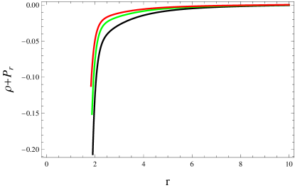
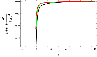
Figure 2: Plots of null energy condition versus $r$ with respect to model 1.

3.2 Model 2

The Starobinsky model is another well-known gravity model consistent with cosmic observations and fulfills the solar system tests. The Starobinsky model is defined as [53]

$$f(R)=R-MC\bigg{[}1-\bigg{(}1+\frac{R^{2}}{C^{2}}\bigg{)}^{-p}\bigg{]}.$$ (31)

This model predicts a particular pattern of gravitational waves and can also reproduce the early cosmic inflation. During this phase, the universe expanded exponentially, which can explain several observed features of the cosmic microwave background radiation. Here, $M$ and $p$ are arbitrary constants. The field equations with respect to the Starobinsky model are

$$\rho = \frac{1}{{e^{\psi}}2(2\gamma+1)(\gamma+1)}\bigg{[}(5\gamma+2)\frac{1}{e^{\psi}}\bigg{\{}-e^{\psi}\big{(}\frac{f}{2}+\frac{q^{2}}{8\pi r^{4}}+\frac{q^{2}}{2r^{4}}\gamma\big{)}$$

$$+ \big{(}\frac{\lambda^{\prime}}{r}-\frac{\lambda^{\prime}\psi^{\prime}}{4}+\frac{\lambda^{\prime\prime}}{2}+\frac{\lambda^{\prime 2}}{4}\big{)}\big{(}1-\frac{2pMR(1+\frac{R^{2}}{C^{2}})^{-1-p}}{C}\big{)}$$

$$+ \big{(}\frac{\psi^{\prime}}{2}-\frac{2}{r}\big{)}\bigg{\{}\frac{2Mp}{C(1+\frac{R^{2}}{C^{2}})^{1+p}}\bigg{(}\frac{-2(1+p)R^{2}}{C^{2}(1+\frac{R^{2}}{C^{2}})}-1\bigg{)}R^{\prime}\bigg{\}}$$

$$- \bigg{\{}\frac{2Mp}{C(1+\frac{R^{2}}{C^{2}})^{1+p}}\bigg{(}\frac{-2(1+p)R^{2}}{C^{2}(1+\frac{R^{2}}{C^{2}})}-1\bigg{)}R^{\prime\prime}+\frac{4pMR}{C^{3}(1+\frac{R^{2}}{C^{2}})^{p+2}}$$

$$\times \bigg{(}(3+3p)-\frac{2(p^{2}+3p+4)R^{2}}{C^{2}(1+\frac{R^{2}}{C^{2}})}\bigg{)}R^{\prime 2}\bigg{\}}\bigg{\}}+\gamma\bigg{\{}e^{\psi}\big{(}\frac{f}{2}+\frac{q^{2}}{8\pi r^{4}}$$

$$+ \frac{q^{2}}{2r^{4}}\gamma\big{)}+\big{(}-\frac{\lambda^{\prime\prime}}{2}+\frac{\psi^{\prime}}{r}+\frac{\lambda^{\prime}\psi^{\prime}}{4}-\frac{\lambda^{\prime 2}}{4}\big{)}\big{(}1-\frac{2pMR(1+\frac{R^{2}}{C^{2}})^{-1-p}}{C}\big{)}$$

$$+ \big{(}\frac{\lambda^{\prime}}{2}+\frac{2}{r}\big{)}\bigg{\{}\frac{2Mp}{C(1+\frac{R^{2}}{C^{2}})^{1+p}}\bigg{(}\frac{-2(1+p)R^{2}}{C^{2}(1+\frac{R^{2}}{C^{2}})}-1\bigg{)}R^{\prime}\bigg{\}}\bigg{\}}$$

$$+ 2\gamma\bigg{\{}e^{\psi}\big{(}\frac{f}{2}-\frac{q^{2}}{8\pi r^{4}}-\frac{q^{2}}{2r^{4}}\gamma\big{)}+\big{(}\frac{(\lambda^{\prime}-\psi^{\prime})r}{2}-e^{\psi}+1\big{)}$$

$$\times \frac{\big{(}-1+\frac{2pMR(1+\frac{R^{2}}{C^{2}})^{-1-p}}{C}\big{)}}{r^{2}}+\bigg{(}\frac{\lambda^{\prime}-\psi^{\prime}}{2}+\frac{1}{r}\big{)}\bigg{\{}\frac{2Mp}{C(1+\frac{R^{2}}{C^{2}})^{1+p}}$$

$$\times \bigg{(}\frac{-2(1+p)R^{2}}{C^{2}(1+\frac{R^{2}}{C^{2}})}-1\bigg{)}R^{\prime}\bigg{\}}+\bigg{\{}\frac{2Mp}{C(1+\frac{R^{2}}{C^{2}})^{1+p}}$$

$$\times \bigg{(}\frac{-2(1+p)R^{2}}{C^{2}(1+\frac{R^{2}}{C^{2}})}-1\bigg{)}R^{\prime\prime}+\frac{4pMR}{C^{3}(1+\frac{R^{2}}{C^{2}})^{p+2}}\bigg{(}3(1+p)$$

$$- \frac{2(p^{2}+3p+4)R^{2}}{C^{2}(1+\frac{R^{2}}{C^{2}})}\bigg{)}R^{\prime 2}\bigg{\}}\bigg{\}}\bigg{]},$$ (32)

$$P_{r} = \frac{1}{{e^{\psi}}2(2\gamma+1)(\gamma+1)}\bigg{[}-\gamma\bigg{\{}-e^{\psi}\big{(}\frac{f}{2}+\frac{q^{2}}{8\pi r^{4}}+\frac{q^{2}}{2r^{4}}\gamma\big{)}$$ (33)

$$+ \big{(}\frac{\lambda^{\prime}}{r}-\frac{\lambda^{\prime}\psi^{\prime}}{4}+\frac{\lambda^{\prime\prime}}{2}+\frac{\lambda^{\prime 2}}{4}\big{)}\big{(}1-\frac{2pMR(1+\frac{R^{2}}{C^{2}})^{-1-p}}{C}\big{)}+\big{(}\frac{\psi^{\prime}}{2}$$

$$- \frac{2}{r}\big{)}\bigg{\{}\frac{2Mp}{C(1+\frac{R^{2}}{C^{2}})^{1+p}}\bigg{(}\frac{-2(1+p)R^{2}}{C^{2}(1+\frac{R^{2}}{C^{2}})}-1\bigg{)}R^{\prime}\bigg{\}}-\bigg{\{}\frac{2Mp}{C(1+\frac{R^{2}}{C^{2}})^{1+p}}$$

$$\times \bigg{(}\frac{-2(1+p)R^{2}}{C^{2}(1+\frac{R^{2}}{C^{2}})}-1\bigg{)}R^{\prime\prime}+\frac{4nMR}{C^{3}(1+\frac{R^{2}}{C^{2}})^{p+2}}\bigg{(}3(1+p)$$

$$- \frac{2(p^{2}+3p+4)R^{2}}{C^{2}(1+\frac{R^{2}}{C^{2}})}\bigg{)}R^{\prime 2}\bigg{\}}\bigg{\}}+(3\gamma+2)\bigg{\{}e^{\psi}\big{(}\frac{f}{2}+\frac{q^{2}}{8\pi r^{4}}$$

$$+ \frac{q^{2}}{2r^{4}}\gamma\big{)}+\big{(}-\frac{\lambda^{\prime\prime}}{2}+\frac{\psi^{\prime}}{r}+\frac{\lambda^{\prime}\psi^{\prime}}{4}-\frac{\lambda^{\prime 2}}{4}\big{)}\big{(}1-\frac{2pMR(1+\frac{R^{2}}{C^{2}})^{-1-p}}{C}\big{)}$$

$$+ \big{(}\frac{\lambda^{\prime}}{2}+\frac{2}{r}\big{)}\bigg{\{}\frac{2Mp}{C(1+\frac{R^{2}}{C^{2}})^{1+p}}\bigg{(}\frac{-2(1+p)R^{2}}{C^{2}(1+\frac{R^{2}}{C^{2}})}-1\bigg{)}R^{\prime}\bigg{\}}\bigg{\}}$$

$$- 2\gamma\bigg{\{}e^{\psi}\big{(}\frac{f}{2}-\frac{q^{2}}{8\pi r^{4}}-\frac{q^{2}}{2r^{4}}\gamma\big{)}+\big{(}\frac{(\lambda^{\prime}-\psi^{\prime})r}{2}-e^{\psi}+1\big{)}$$

$$\times \frac{\big{(}-1+\frac{2pMR(1+\frac{R^{2}}{C^{2}})^{-1-p}}{C}\big{)}}{r^{2}}+\big{(}\frac{\lambda^{\prime}-\psi^{\prime}}{2}+\frac{1}{r}\big{)}\bigg{\{}\frac{2Mp}{C(1+\frac{R^{2}}{C^{2}})^{1+p}}$$

$$\times \bigg{(}\frac{-2(1+p)R^{2}}{C^{2}(1+\frac{R^{2}}{C^{2}})}-1\bigg{)}R^{\prime}\bigg{\}}+\bigg{\{}\frac{2Mp}{C(1+\frac{R^{2}}{C^{2}})^{1+p}}$$

$$\times \bigg{(}\frac{-2(1+p)R^{2}}{C^{2}(1+\frac{R^{2}}{C^{2}})}-1\bigg{)}R^{\prime\prime}+\frac{4pMR}{C^{3}(1+\frac{R^{2}}{C^{2}})^{p+2}}\bigg{(}3(1+p)$$

$$- \frac{2(p^{2}+3p+4)R^{2}}{C^{2}(1+\frac{R^{2}}{C^{2}})}\bigg{)}R^{\prime 2}\bigg{\}}\bigg{\}}\bigg{]},$$

$$P_{t} = \frac{1}{{e^{\psi}}2(2\gamma+1)(\gamma+1)}\bigg{[}-\gamma\bigg{\{}-e^{\psi}\big{(}\frac{f}{2}+\frac{q^{2}}{8\pi r^{4}}+\frac{q^{2}}{2r^{4}}\gamma\big{)}$$ (34)

$$+ \big{(}\frac{\lambda^{\prime}}{r}-\frac{\lambda^{\prime}\psi^{\prime}}{4}+\frac{\lambda^{\prime\prime}}{2}+\frac{\lambda^{\prime 2}}{4}\big{)}\big{(}1-\frac{2pMR(1+\frac{R^{2}}{C^{2}})^{-1-p}}{C}\big{)}+\big{(}\frac{\psi^{\prime}}{2}-\frac{2}{r}\big{)}$$

$$\times \bigg{\{}\frac{2Mp}{C(1+\frac{R^{2}}{C^{2}})^{1+p}}\bigg{(}\frac{-2(1+p)R^{2}}{C^{2}(1+\frac{R^{2}}{C^{2}})}-1\bigg{)}R^{\prime}\bigg{\}}-\bigg{\{}\frac{2Mp}{C(1+\frac{R^{2}}{C^{2}})^{1+p}}$$

$$\times \bigg{(}\frac{-2(1+p)R^{2}}{C^{2}(1+\frac{R^{2}}{C^{2}})}-1\bigg{)}R^{\prime\prime}+\frac{4pMR}{C^{3}(1+\frac{R^{2}}{C^{2}})^{p+2}}\bigg{(}3(1+p)$$

$$- \frac{2(p^{2}+3p+4)R^{2}}{C^{2}(1+\frac{R^{2}}{C^{2}})}\bigg{)}R^{\prime 2}\bigg{\}}\bigg{\}}+\gamma\bigg{\{}e^{\psi}\big{(}\frac{f}{2}+\frac{q^{2}}{8\pi r^{4}}+\frac{q^{2}}{2r^{4}}\gamma\big{)}$$

$$+ \big{(}-\frac{\lambda^{\prime\prime}}{2}+\frac{\psi^{\prime}}{r}+\frac{\lambda^{\prime}\psi^{\prime}}{4}-\frac{\lambda^{\prime 2}}{4}\big{)}\big{(}1-\frac{2pRM(1+\frac{R^{2}}{C^{2}})^{-1-p}}{C}\big{)}$$

$$+ \big{(}\frac{\lambda^{\prime}}{2}+\frac{2}{r}\big{)}\bigg{\{}\frac{2Mp}{C(1+\frac{R^{2}}{C^{2}})^{1+p}}\bigg{(}\frac{-2(1+p)R^{2}}{C^{2}(1+\frac{R^{2}}{C^{2}})}-1\bigg{)}R^{\prime}\bigg{\}}\bigg{\}}$$

$$- 2(\gamma+1)\bigg{\{}e^{\psi}\big{(}\frac{f}{2}-\frac{q^{2}}{8\pi r^{4}}-\frac{q^{2}}{2r^{4}}\gamma\big{)}+\big{(}\frac{(\lambda^{\prime}-\psi^{\prime})r}{2}-e^{\psi}+1\big{)}$$

$$\times \frac{\big{(}-1+\frac{2pMR(1+\frac{R^{2}}{C^{2}})^{-1-p}}{C}\big{)}}{r^{2}}+\big{(}\frac{\lambda^{\prime}-\psi^{\prime}}{2}+\frac{1}{r}\big{)}\bigg{\{}\frac{2Mp}{C(1+\frac{R^{2}}{C^{2}})^{1+p}}$$

$$\times \bigg{(}\frac{-2(1+p)R^{2}}{C^{2}(1+\frac{R^{2}}{C^{2}})}-1\bigg{)}R^{\prime}\bigg{\}}+\bigg{\{}\frac{2Mp}{C(1+\frac{R^{2}}{C^{2}})^{1+p}}$$

$$\times \bigg{(}\frac{-2(1+p)R^{2}}{C^{2}(1+\frac{R^{2}}{C^{2}})}-1\bigg{)}R^{\prime\prime}+\frac{4pMR}{C^{3}(1+\frac{R^{2}}{C^{2}})^{p+2}}\bigg{(}3(1+p)$$

$$- \frac{2(p^{2}+3p+4)R^{2}}{C^{2}(1+\frac{R^{2}}{C^{2}})}\bigg{)}R^{\prime 2}\bigg{\}}\bigg{\}}\bigg{]}.$$

Figure 3 shows that the null energy condition is violated for $p=-7,~{}M=1,~{}C=-23$, (black color), $p=-7.5,~{}M=-1,~{}C=-22$ (green color), $p=-8,~{}M=1.8,~{}C=-21$ (red color). Hence we obtain traversable spherically symmetric WH geometry.

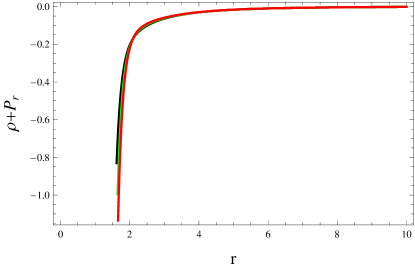
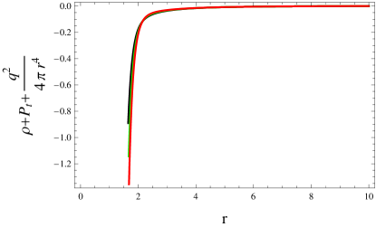
Figure 3: Plots of null energy condition versus $r$ with respect to model 2.

4 Stability Analysis

Stability is a crucial factor while analyzing cosmic structures such as star clusters, and even the universe as a whole. The stability of cosmic structures provides insights into the underlying physics and processes that govern their behavior. Stable structures are those that maintain their shape and properties over time, despite any external influences or disturbances. Studying these objects can help scientists to better understand the distribution of matter in the universe, the formation and evolution of galaxies clusters and the nature of dark components. Here, we use sound speed to check the stability of our obtained WH geometry.

We use the causality and Herrera cracking techniques to examine the stability of WH under the influence of charge. The causality constraint states that no information or signal can propagate faster than the speed of light. This condition implies that the speed of sound components $(v^{2}_{r}=\frac{dP_{r}}{d\rho},~{}v_{t}^{2}=\frac{dP_{t}}{d\rho})$ must lie between $[0,1]$ for stable cosmic structure. From Figure 4, we can see that the causality condition is satisfied for our obtained WH solutions under the influence of charge and dark source terms. Herrera cracking is another method that considers the WH as a thin-shell and analyzes the behavior of stress under various perturbations. Herrera cracking method states that the difference between the sound speed components $v_{t}^{2},~{}v^{2}_{r}$ must lie between $0$ to $1$. The graphical behavior is presented in Figure 5, which determines that our obtained WH solutions satisfies all the necessary criteria of stability. Hence, physically viable and stable WH solutions exist in $f(R,T)$ theory.

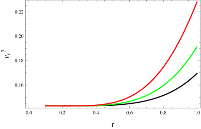
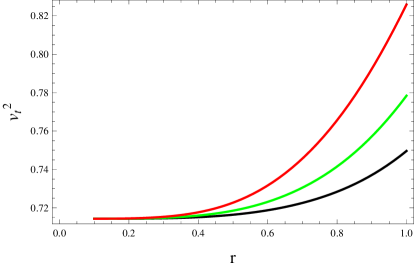
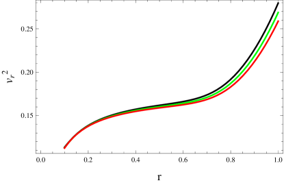
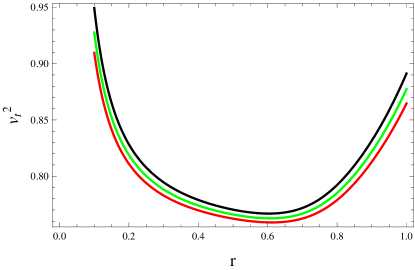
Figure 4: Plots of causality condition versus radial coordinate with respect to models 1 and 2.

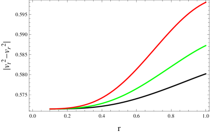
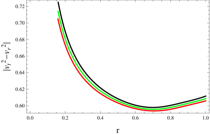
Figure 5: Plots of Herrera cracking versus radial coordinate with respect to models 1 and 2.

5 Final Remarks

In the literature, there are several approaches that have been used to find viable WH solutions. One common approach for evaluating the shape function is to make certain assumptions about the matter ingredients. These assumptions can be used to explore the Einstein field equations and derive the shape function for the WH structure. Another approach is to consider a shape function to examine the behavior of energy bounds. The energy conditions can be used to derive important physical properties of the object. In this paper, we have studied the effects of charge on viable WH geometry in $f(R,T)$ gravity. For this, we have built a shape function by employing the Karmarkar condition. We have assumed exponential gravity and Starobinsky gravity models of this gravity to analyze the viability and stability of WH solutions. The viability of obtained WH solutions is analyzed by null energy condition, and their stable state is checked through the speed of sound. The obtained results are summarized as follows

• We have shown that our developed shape function is physically viable as it satisfies all the necessary conditions (Figure 1).

• For the exponential gravity model, the null energy condition is violated, and exotic matter exists in the WH vicinity for $L>0$ and $C<0$. Thus we have obtained the viable traversable WH geometry for specific values of $L$ and $C$.

• The null energy condition is violated for $C<0$, $M>0$ and $p<0$ corresponding to Starobinsky gravity model (Figure 3). This manifests that the interior region of WH throat is filled with exotic matter, which leads to the viable traversable WH geometry.

• We have found that all the required constraints of stability are fulfilled under the influence of charge in $f(R,T)$ theory (Figures 4 and 5).

It is important to note here that our obtained solutions are more stable in the presence of charge as compared to that found in the absence of electromagnetic field [45, 46].

References

• [1] Perlmutter, S. et al.: Astrophys. J. 483(1997)565; Nature 391(1998)51; Astrophys. J. 517(1999)565.
• [2] Nojiri, S. and Odintsov, S.D.: Phys. Rev. D 68(2003)123512.
• [3] Song, Y.S., Hu, W. and Sawicki, I.: Phys. Rev. D 75(2007)044004.
• [4] Akbar, M. and Cai, R.G.: Phys. Lett. B 648(2007)243.
• [5] Nojiri, S. and Odintsov, S.D.: Phys. Rep. 505(2011)59.
• [6] Harko, T. et al.: Phys. Rev. D 84(2011)024020.
• [7] Jamil, M. et al.: Eur. Phys. J. C 72(2012)1999.
• [8] Santos, A.F.: Mod. Phys. A 28(2013)1350141.
• [9] Sharif, M. and Zubair, M.: J. Phys. Soc. Jpn. 82(2013)064001.
• [10] Singh, C.P. and Singh, V.: Gen. Relativ. Gravit. 46(2014)1696.
• [11] Shabani, H. and Farhoudi, M.: Phys. Rev. D 90(2014)044031.
• [12] Noureen, I. and Zubair, M.: Eur. Phys. J. C 75(2015)62.
• [13] Moraes, P.H.R.S.: Eur. Phys. J. C 75(2015)168.
• [14] Zubair, M. and Noureen, I.: Eur. Phys. J. C 75(2015)265.
• [15] Noureen, I. et al.: Eur. Phys. J. C 75(2015)323.
• [16] Sharif, M. and Gul, M.Z.: Mod. Phys. Lett. A 36(2021)21502014.
• [17] Sharif, M. and Waseem, A.: Eur. Phys. J. C 78(2018)868.
• [18] Flamm, L.: Phys. Z. 17(1916)448.
• [19] Einstein, A. and Rosen, N.: Phys. Rev. 48(1935)73.
• [20] Wheeler, J.A.: Phys. Rev. 97(1955)511.
• [21] Ellis, H.G.: J. Math. Phys. 14(1973)104.
• [22] Morris, M.S. and Thorne, L.S.: Am. J. Phys. 56(1988)395.
• [23] Visser, M.: Phys. Rev. D 39(1989)3182.
• [24] Visser, M. and Wormholes, L.: From Einstein to Hawking (American Institute of Physics, 1996).
• [25] Sushkov, S.: Phys. Rev. D 71(2005)043520.
• [26] Lobo, F.S.N.: Phys. Rev. D 71(2005)084011.
• [27] Eiroa, E.F. and Simeone, C.: Phys. Rev. D 82(2010)084039.
• [28] Richarte, M.G.: Phys. Rev. D 88(2013)027507.
• [29] Bronnikov, K.A. and Skvortsova, M.V.: Grav. Cosmol. 20(2014)171.
• [30] Gibbons, G.W. and Volkov, M.S.: J. Cosmol. Astropart. Phys. 2017(2017)039.
• [31] Lemos, J.P.S., Lobo, F.S.N. and de Oliveira, S.Q.: Phys. Rev. D 68(2003)064004; Fayyaz, I. and Shamir, M.F.: Chin. J. Phys. 66(2020)553.
• [32] Sharif, M. and Fatima, I.: Gen. Relativ. Gravit. 48(2016)148.
• [33] Cataldo, M., Liempi, L. and Rodriguez, P.: Eur. Phys. J. C 77(2017)748.
• [34] Godani, N. and Samanta, G.C.: Int. J. Mod. Phys. D 28(2019)1950039.
• [35] Sharif, M. and Gul, M.Z.: Symmetry 15(2023)684.
• [36] Esculpi, M. and Aloma, E.: Eur. Phys. J. C 67(2010)521.
• [37] Sharif, M. and Mumtaz, S.: Astrophys. Space Sci. 352(2014)729.
• [38] Moraes, P.H.R.S., Paula, W.D. and Correa, R.A.C.: Int. J. Mod. Phys. D 28(2019)1950098.
• [39] Sharif, M. and Naz, S.: Mod. Phys. Lett. A 35(2020)1950340.
• [40] Sharif, M. and Javed, F.: Astron. Rep. 65(2021)353.
• [41] Elizalde, E. and Khurshudyan, M.: Phys. Rev. D 98(2018)123525.
• [42] Sharif, M. and Hussain, S.: Chin. J. Phys. 61(2019)194.
• [43] Shamir, M.F. and Fayyaz, I.: Eur. Phys. J. C 80(2020)1102.
• [44] Mishra, B. at al.: Int. J. Mod. Phys. D 30(2021)2150061.
• [45] Shamir. M.F., Malik, A. and Mustafa, G.: Chin. J. Phys. 73(2021)634.
• [46] Sharif, M. and Fatima, A.: Eur. Phys. J. Plus 138(2023)196.
• [47] Anchordoqui, L.A. et al.: Phys. Rev. D 57(1998)829.
• [48] Sharif, M. and Siddiqa, A.: Eur. Phys. J. Plus 132(2017)529.
• [49] Haghani, Z. et al.: Phys. Rev. D 88(2013)044023.
• [50] Cognola, G. et al.: Phys. Rev. D 77(2008)046009.
• [51] de Felice, F., Yu, Y. and Fang, J.: Mon. Not. R. Astron. Soc. 277(1995)L17.
• [52] Deb, D. et al.: J. Cosmol. Astropart. Phys. 2019(2019)070.
• [53] Starobinsky, A.A.: J. Exp. Theor. Phys. 86(2007)157.