Refrigeration by modified Otto cycles and modified swaps through generalized measurements

Abstract

We introduce two types of thermodynamic refrigeration cycles obtained through modification of the Otto cycle refrigerator by a generalized measurement channel. These refrigerators are corresponding to the activation of the measurement-based stroke before (first type) and after (second type) the full thermalization of the cooling medium by the cold reservoir in the related familiar Otto cycle. We show that the coefficient of performance for the first type modified refrigerator increases linearly in terms of measurement strength parameter, beyond the classical cooling of the known Otto cycle refrigerator. The second type interestingly introduces another autonomous refrigerator whose supplying work is provided by a quantum engine induced by the measurement channel along the modified cycle. By the considered measurement channel, we also establish such modifications on the swap refrigerator. It is observed that the thermodynamic properties of the obtained modified swap refrigerators are the same as of the modified Otto cycle ones respectively.


Keywords: Modified Otto cycle refrigerator, Modified swap refrigerator, Coefficient of performance, Generalized measurement, Measurement strength parameter, Autonomous refrigerator

I. Introduction

The main landscape of quantum thermodynamics is concerned with how the effect of quantum resources such as coherence, entanglement and quantum measurement on the quality of work extraction, refrigeration, etc, in thermal devices can be understood and applied [1-5]. As is well-known, quantum measurements are able to alter the average energy and entropy of a quantum system, provided that the measured observable does not commute with the Hamiltonian of that system [6-10]. Thus they can play similar role as thermal reservoirs. The measurement-driven devices which use energetic fluctuations generated by quantum measurement, have recently been explored [5, 9-14].

On the other hand, in Ref. [15], a three-stroke quantum engine on the basis of non-selective generalized measurement channels with adjustable measurement strengths has been proposed and later, by employing nuclear magnetic resonance (NMR) platform, it has been realized experimentally [16]. An interesting advantage of the introduced engine in [15] which was also observed in the experimental results reported in [16], is that this kind of quantum engine can reach unit efficiency while also achieving maximum extracted power at the same time with the fine-tuning of the measurement strengths parameter. The approach of [15] then was developed to introduce another measurement-based devices such as refrigerator and thermal accelerator according to a measurement setting intensity [17].

The other feature of measurement channels introduced in [15] is that their implementation running time is much smaller than any decoherence or thermalization time scales [16]. This property along with the adjustable measurement strength, encourage one to involve this type of measurement channel, as a quantum resource, in the known thermodynamics cycles such as Otto cycle and swap, as an additional stroke. Involving the thermodynamics cycles with this additional stroke, called as modified cycles, may lead the obtained devices to have surpassing properties relative to the traditional ones.

In this work, we perform two types of modifications on the known Otto cycle using a generalized measurement channel similar to the one introduced in [15], as an additional stroke. As is well-known in the known Otto cycle, a quantum system, particularly a two-level one considered as cooling medium (CM), undergoes two isochoric strokes and two adiabatic ones. The modifications on the Otto cycle refrigerator are obtained whenever the measurement-based stroke is exploited before (first type) and after (second type) the full thermalization of two-level system with the cold thermal reservoir. The first type modification leads to a refrigerator whose coefficient of performance (COP) increases in terms of measurement strength parameter beyond the case related to the Otto cycle refrigerator, which is a genuine quantum effect. In fact, for a given value of external work, the COP of modified Otto cycle refrigerator goes beyond the Otto cycle one depending on the intensity of measurement-based stroke. The second type modification interestingly leads to another type of quantum autonomous refrigerator which by itself have been subject of researches in last years [18-29]. In general, a refrigerator is autonomous in the sense that it does not require any external sources of work for cooling. The process which we are encountered in the obtained refrigerator by the second modification, is a quantum effect because the required work for the refrigeration is supplied by the extracted work from a three-stroke quantum engine induced by the measurement-based stroke in the modified Otto cycle. It is interesting to note that the efficiency of measurement-induced quantum engine is the same as of an Otto cycle engine such that all of its three strokes depend directly on the measurement strength parameter.

The modification scheme described on the Otto cycle refrigerator can be applied easily on the two-stroke swap refrigerator. As the previous case, we can obtain two types of three-stroke modified swap refrigerators depending on that the measurement-based stroke activated before (first type) or after (second type) the swap operation. These types of modifications lead to refrigerators which have the same properties as of the discussed modified Otto cycle refrigerators respectively.

II. Refrigeration by first type modified Otto cycle

In a four-stroke Otto cycle refrigerator, a given amount of work that is spent by an external agent on the CM during two adiabatic strokes causes remove of an amount of heat from the cold reservoir and in return flow of another amount of heat into the hot reservoir during two isochoric strokes. In this section, by considering the known Otto cycle which is in the refrigeration mode, we involve a measurement apparatus into it before full thermalization of the CM by the cold reservoir. We show that the obtained modified refrigerator makes remove of more heat from the cold reservoir for the same amount of invested work. To this aim, let us consider the CM is a two-level system with Hamiltonian $H=\frac{\omega}{2}\sigma_{z}$ where $\sigma_{z}$ is the z-component Pauli spin-$\frac{1}{2}$ operator and $\omega$ is the corresponding transition frequency. In general, a measurement apparatus (channel) makes generalized measurements on the CM described by completely positive and trace-preserving (CPTP) maps [30]. To describe the first type modified Otto cycle refrigerator, let us introduce a particular measurement on the CM represented by the following measurement operators with adjustable measurement strength [15], as follows

$$M_{1}(\mathcal{\xi})=|0\rangle\langle 0|+\sqrt{1-\mathcal{\xi}}|1\rangle\langle 1|,\qquad M_{2}(\mathcal{\xi})=\sqrt{\mathcal{\xi}}|0\rangle\langle 1|,$$ (1)

where $\mathcal{\xi}$ is the measurement strength parameter. Obviously the operators $M_{1}(\mathcal{\xi})$ and $M_{2}(\mathcal{\xi})$ satisfy $\Sigma_{i}M_{i}(\mathcal{\xi})^{\dagger}M_{i}(\mathcal{\xi})=I$ which in fact, is the essence of fundamental theorem of quantum measurement [30]. In addition, the operators $E_{1}(\xi):=M_{1}(\mathcal{\xi})^{\dagger}M_{1}(\mathcal{\xi})=|0\rangle\langle 0|+\left(1-\mathcal{\xi}\right)|1\rangle\langle 1|$ and $E_{2}(\xi):=M_{2}(\mathcal{\xi})^{\dagger}M_{2}(\mathcal{\xi})=\mathcal{\xi}|1\rangle\langle 1|$ are the so-called POVM (positive operator valued measure) operators corresponding to the measurement operators (1). It is clear that, $0\leq\mathcal{\xi}\leq 1$, where $\mathcal{\xi}=0$ indicates that the system has not been disturbed (measured) by the measurement process, and $\mathcal{\xi}=1$ corresponds to performing strong or projective measurement on the CM.

To achieve first modification on the Otto cycle refrigerator (Fig. 1), let us assume that the CM, at the beginning, is in the thermal equilibrium with the cold reservoir whose inverse temperature is $\beta_{c}$. In this time, the Hamiltonian of the CM is denoted by $H_{c}=\frac{\omega_{c}}{2}\sigma_{z}$ where $\omega_{c}$ is the corresponding transition frequency in this situation. So the corresponding Gibbs state of the CM is denoted by $\rho_{c}=e^{-\beta_{c}H_{c}}/\mathcal{Z}_{c}$, where $\mathcal{Z}_{c}=Tr[e^{-\beta_{c}H_{c}}]$ is the partition function. The mean energy, in this step, is equal to $E_{1}=Tr[H_{c}\rho_{c}]=-\frac{\omega_{c}}{2}\mathrm{tanh}\left(\beta_{c}\omega_{c}/2\right)$. To describe the 1st stroke, we let the CM is isolated from the cold reservoir and undergoes adiabatic unitary evolution in which only the transition frequency (for simplicity and without lose of generality) changes from $\omega_{c}$ to $\omega_{h}$ such that $\omega_{c}<\omega_{h}$. Therefore, the mean energy after this stroke is obtained as $E_{2}=Tr[H_{h}\rho_{c}]=-\frac{\omega_{h}}{2}\mathrm{tanh}\left(\beta_{c}\omega_{c}/2\right)$ where $H_{h}=\frac{\omega_{h}}{2}\sigma_{z}$.

The 2nd stroke is provided by full thermalization of the CM by a hot thermal reservoir with inverse temperature $\beta_{h}$ $(\beta_{h}<\beta_{c})$. In this time the corresponding Gibbs state is given by $\rho_{h}=e^{-\beta_{h}H_{h}}/\mathcal{Z}_{h}$ where $\mathcal{Z}_{h}=Tr[e^{-\beta_{h}H_{h}}]$ is the partition function. By this stroke, the mean energy is changed from $E_{2}$ to $E_{3}$ which is equal to $E_{3}=Tr[H_{h}\rho_{h}]=-\frac{\omega_{h}}{2}\mathrm{tanh}\left(\beta_{h}\omega_{h}/2\right)$. In the 3rd stroke, which is similar to the first one, the CM is isolated from the hot reservoir and undergoes adiabatically unitary evolution in which the transition frequency is brought, in an isentropic way, to the original value $\omega_{c}$. The corresponding mean energy becomes as $E_{4}=Tr[H_{c}\rho_{h}]=-\frac{\omega_{c}}{2}\mathrm{tanh}\left(\beta_{h}\omega_{h}/2\right)$.

The promised modification for the known Otto cycle refrigerator is introduced by effect of the 4th stroke on the CM in which it is left to interact with a measurement apparatus such that its effect is corresponding to the effect of a non-selective generalized measurement on the CM as $\mathcal{E}(\rho_{h})=\Sigma_{i}M_{i}(\xi)\rho_{h}M_{i}^{\dagger}(\xi)$ where $M_{i}(\xi)$s are the measurement operators defined in Eq. (1). Therefore the mean energy takes the following value as

$$E_{5}=Tr[H_{c}\rho_{{}_{h}}(\mathcal{\xi})]=-\frac{\omega_{c}}{2}\mathrm{tanh}\left(\beta_{h}\omega_{h}/2\right)-\mathcal{\xi}\omega_{c}\frac{e^{-\beta_{h}\omega_{h}/2}}{\mathcal{Z}_{h}},$$ (2)

where

$$\mathcal{E}(\rho_{h}):=\rho_{{}_{h}}(\mathcal{\xi})=\frac{1}{\mathcal{Z}_{h}}\left[(1-\mathcal{\xi})e^{{-\beta_{h}\omega_{h}/2}}|1\rangle\langle 1|+(e^{{\beta_{h}\omega_{h}/2}}+\mathcal{\xi}e^{{-\beta_{h}\omega_{h}/2}})|0\rangle\langle 0|\right].$$ (3)

It is clear that $\rho_{{}_{h}}(\mathcal{\xi})$ is a non-equilibrium passive state with no induced ergotropy [31], by the measurement apparatus. Consequently, the cycle is completed by 5th stroke which is the thermalization of the CM by the cold reservoir. By considering the condition $\beta_{c}\omega_{c}<\beta_{h}\omega_{h}$, the CM throughout the modified Otto cycle exchanges following works and heats with work and heat sources as well as with the measurement apparatus as

$$1\mathrm{st}\quad\mathrm{stroke}:\quad W_{1}=E_{2}-E_{1}=\left(\frac{\omega_{c}-\omega_{h}}{2}\right)\mathrm{tanh}\left(\frac{\beta_{c}\omega_{c}}{2}\right),$$ (4)

$$2\mathrm{nd}\quad\mathrm{stroke}:\quad Q_{h}=E_{3}-E_{2}=\frac{\omega_{h}}{2}\left[\mathrm{tanh}\left(\frac{\beta_{c}\omega_{c}}{2}\right)-\mathrm{tanh}\left(\frac{\beta_{h}\omega_{h}}{2}\right)\right],$$ (5)

$$3\mathrm{rd}\quad\mathrm{stroke}:\quad W_{2}=E_{4}-E_{3}=\left(\frac{\omega_{h}-\omega_{c}}{2}\right)\mathrm{tanh}\left(\frac{\beta_{h}\omega_{h}}{2}\right),$$ (6)

$$4\mathrm{th}\quad\mathrm{stroke}:\quad Q(\xi)=E_{5}-E_{4}=-\mathcal{\xi}\omega_{c}\frac{e^{-\beta_{h}\omega_{h}/2}}{\mathcal{Z}_{h}},$$ (7)

$$5\mathrm{th}\quad\mathrm{stroke}:\quad Q_{c}(\xi)=E_{1}-E_{5}=Q_{c}-Q(\xi),$$ (8)

where

$$Q_{c}=\frac{\omega_{c}}{2}\left[\mathrm{tanh}\left(\frac{\beta_{h}\omega_{h}}{2}\right)-\mathrm{tanh}\left(\frac{\beta_{c}\omega_{c}}{2}\right)\right].$$ (9)

$Q_{h}<0$ ($Q(\xi)<0$) is the amount of heat (quantum heat [5, 15]) flowed from the CM into the hot reservoir (measurement apparatus) while $Q_{c}(\xi)>0$ is as heat flowed from the cold reservoir into the CM (Fig. 1). Also the work $W_{1}<0$ is extracted from the CM while $W_{2}>0$ is invested on it as depicted in Fig. 1. Clearly in the absence the measurement process $(\xi=0)$ then the received heat by the CM from the cold reservoir is reduced to $Q_{c}$ which is corresponding to the case of Otto cycle refrigerator. The COP for the corresponding modified refrigerator is obtained as follows

$$\mathrm{COP}(\xi)=\frac{Q_{c}(\xi)}{W_{in}}=\left(\frac{\omega_{h}}{\omega_{c}}-1\right)^{-1}\left(1+\frac{2\mathcal{\xi}}{\mathcal{Z}_{h}}\frac{e^{-\beta_{h}\omega_{h}/2}}{\left[\mathrm{tanh}\left(\frac{\beta_{h}\omega_{h}}{2}\right)-\mathrm{tanh}\left(\frac{\beta_{c}\omega_{c}}{2}\right)\right]}\right),$$ (10)

where

$$W_{\mathrm{in}}=W_{1}+W_{2}=\left(\frac{\omega_{h}-\omega_{c}}{2}\right)\left[\mathrm{tanh}\left(\frac{\beta_{h}\omega_{h}}{2}\right)-\mathrm{tanh}\left(\frac{\beta_{c}\omega_{c}}{2}\right)\right],$$ (11)

is the required work $(W_{\mathrm{in}}>0)$ for the refrigeration which should be invested on the CM by an external agent to enforce flow of heat from the cold reservoir into the hot one and the measurement apparatus. It is clear that when the measurement strength parameter becomes zero, i.e $\mathcal{\xi}=0$, then the COP in Eq. (10), leads to the one of the familiar Otto cycle refrigerator.

Fig. 2, shows the COP for the modified refrigerator in terms of measurement strength parameter $\xi$, for various amounts of invested work. In fact, for each values of invested works, the COP is always a linearly increasing function of $\xi$, beyond the one of the familiar Otto cycle, such that the rate of its increment is proportional inversely with the values of the invested works. Therefore, the involution of generalized measurement (1) into the Otto cycle, as a quantum resource, leads to the supremacy of the refrigeration process by the introduced (first type) modified Otto cycle with respect to the classical cooling of the Otto cycle refrigerator. On the other hand, the cooling process characterized by the amount of removal heat from the cold reservoir, i.e. $Q_{c}(\xi)$ (see Eq. (9)), is also an increasing function of $\xi$ (Fig. 3), however, it is interesting to note that as $\xi\rightarrow 1$, which is corresponding to the strong measurement case, the cooling process, apart from the values of the invested work, reaches to a unique value.

III. Refrigeration by second type modified Otto cycle

Let us consider the other type of modified Otto cycle obtained by activation of the measurement channel after the full thermalization of the CM by the cold reservoir, as shown in Fig. 4. The 1st stroke causes flow of quantum heat from the two-level system into the measurement apparatus calculated as follows

$$Q(\xi)=E_{2}-E_{1}=-\xi\omega_{c}\frac{e^{-\beta_{c}\omega_{c}/2}}{\mathcal{Z}_{c}}<0,$$ (12)

where $E_{1}=Tr[H_{c}\rho_{c}]$, as the previous case, is the mean energy at the beginning of the 1st stroke and

$$E_{2}=Tr[H_{c}\rho_{c}(\xi)]=-\frac{\omega_{c}}{2}\mathrm{tanh}\left(\frac{\beta_{c}\omega_{c}}{2}\right)-\xi\omega_{c}\frac{e^{-\beta_{c}\omega_{c}/2}}{\mathcal{Z}_{c}},$$ (13)

is at the end of it, with

$$\rho_{c}(\xi)=\frac{1}{\mathcal{Z}_{c}}\left[(1-\xi)e^{{-\beta_{c}\omega_{c}/2}}|1\rangle\langle 1|+(e^{{\beta_{c}\omega_{c}/2}}+\xi e^{{-\beta_{c}\omega_{c}/2}})|0\rangle\langle 0|\right].$$ (14)

Obviously the non-equilibrium state (14), is a passive state without ergotropy. The 2nd stroke causes evolution of the CM unitarily and adiabatically such that only its transition frequency is changed from $\omega_{c}$ to $\omega_{h}$ $(\omega_{c}<\omega_{h})$. Therefore, the mean energy at the end of this stroke becomes

$$E_{3}=Tr[H_{h}\rho_{c}(\xi)]=-\frac{\omega_{h}}{2}\mathrm{tanh}\left(\frac{\beta_{c}\omega_{c}}{2}\right)-\mathcal{\xi}\omega_{h}\frac{e^{-\beta_{c}\omega_{c}/2}}{\mathcal{Z}_{c}},$$ (15)

where, as previously, $H_{h}=\frac{\omega_{h}}{2}\sigma_{z}$. The extracted work from the CM through this stroke is written as

$$\mathcal{W}(\xi)=E_{3}-E_{2}=W_{1}+W(\xi),$$ (16)

where

$$W_{1}=\left(\frac{\omega_{c}-\omega_{h}}{2}\right)\mathrm{tanh}\left(\frac{\beta_{c}\omega_{c}}{2}\right),$$ (17)

and

$$W(\xi)=\mathcal{\xi}(\omega_{c}-\omega_{h})\frac{e^{-\beta_{c}\omega_{c}/2}}{\mathcal{Z}_{c}}.$$ (18)

$\mathcal{W}(\xi)$ is always negative because $W_{1}$ and $W(\xi)$ are always negative. The expression (18), as a part of the extracted work in Eq. (16), originates only from the measurement process such that $\mathcal{W}(\xi=0)=W_{1}$. On the other hand, by the 3rd stroke, our two-level system is brought into contact with the hot thermal reservoir and during this process the amount of exchanged heat becomes as below

$$Q_{h}(\xi)=E_{4}-E_{3}=Q_{h}+Q^{\prime}(\xi),$$ (19)

where

$$Q_{h}=\frac{\omega_{h}}{2}\left[\mathrm{tanh}\left(\frac{\beta_{c}\omega_{c}}{2}\right)-\mathrm{tanh}\left(\frac{\beta_{h}\omega_{h}}{2}\right)\right],$$ (20)

$$Q^{\prime}(\xi)=\xi\omega_{h}\frac{e^{-\beta_{c}\omega_{c}/2}}{\mathcal{Z}_{c}}>0.$$ (21)

and $E_{4}=Tr[H_{h}\rho_{h}]$. By considering the refrigeration condition for the modified Otto cycle, i.e. $\beta_{c}\omega_{c}<\beta_{h}\omega_{h}$, we have $Q_{h}<0$. Thus by this stroke, there is flow of heat $Q_{h}$ from the CM into the hot reservoir and at the same time, flow of quantum heat $Q^{\prime}(\xi)$ from the hot reservoir into the CM, which is only originated from the effect of quantum measurement exploited in the 1st stroke. In the 4th stroke, the Hamiltonian of the CM is returned to its original form, i.e. only its transition frequency is changed from $\omega_{h}$ to $\omega_{c}$, by a unitary and adiabatic process. The invested work, by this stroke, on the CM is calculated as

$$W_{2}=E_{5}-E_{4}=\left(\frac{\omega_{h}-\omega_{c}}{2}\right)\mathrm{tanh}\left(\frac{\beta_{h}\omega_{h}}{2}\right),$$ (22)

where $W_{2}>0$ and $E_{5}=Tr[H_{c}\rho_{h}]$. Ultimately, the CM is brought again into contact with the cold reservoir and the cycle is completed by this (5th) stroke so the amount of heat flowed from the cold reservoir into the CM is obtained as follows

$$Q_{c}=E_{1}-E_{5}=\frac{\omega_{c}}{2}\left[\mathrm{tanh}\left(\frac{\beta_{h}\omega_{h}}{2}\right)-\mathrm{tanh}\left(\frac{\beta_{c}\omega_{c}}{2}\right)\right],$$ (23)

where $Q_{c}>0$. The net work which should be invested by an external agent on the CM, throughout the modified cycle, is

$$W_{ex}(\xi)=W_{in}+W(\xi)=\left(\frac{\omega_{h}-\omega_{c}}{2}\right)\left[\mathrm{tanh}\left(\frac{\beta_{h}\omega_{h}}{2}\right)-\mathrm{tanh}\left(\frac{\beta_{c}\omega_{c}}{2}\right)-2\xi\frac{e^{-\beta_{c}\omega_{c}/2}}{\mathcal{Z}_{c}}\right],$$ (24)

where $W_{ex}(\xi)\geq 0$. On the other hand, $W_{in}=-(Q_{h}+Q_{c})=W_{ex}(\xi)-W(\xi)$ is the amount of work required to invest on the CM in order to remove the heat $Q_{c}$ from the cold reservoir and transfer the heat $Q_{h}$ into the hot reservoir. It is explicitly independent from the measurement-based stroke whereas $W_{ex}(\xi)$ and $W(\xi)$ are not. The COP for the refrigeration on the basis of modified Otto cycle is

$$\mathrm{COP}(\xi)=\frac{Q_{c}}{W_{ex}(\xi)-W(\xi)},$$ (25)

which is also independent from the measurement-based stroke too, and as is evident, it is the same as COP of familiar Otto cycle refrigerator. So what does measurement do really? To answer to this question, let us at first consider the case that the measurement process (1) has not been activated, i.e. $\xi=0$. In this case $W(\xi=0)=0$ so $W_{in}=W_{ex}(\xi=0)$, thus the required work for the refrigeration is provided only by an external agent.

Now, in the presence of measurement-based stroke, i.e. $\xi\neq 0$, it is observed a measurement-induced quantum engine whose operation along the modified cycle consists of absorption of heat $Q^{\prime}(\xi)$ from the hot reservoir and transfer a part of it, i.e. $Q(\xi)$, into the measurement apparatus along with extraction of work $W(\xi)$ such that $W(\xi)=-(Q^{\prime}(\xi)+Q(\xi))$ (Fig. 4). Evidently, the efficiency of this quantum engine is the same as of the familiar Otto cycle heat engine. The extracted work can be regarded (by a suitable feedback) as a part of required work for the refrigeration so the remainder part is supplied by an external agent ($W_{in}=W_{ex}(\xi)-W_{ex}(\xi)$). Furthermore, since $W_{ex}(\xi)$ is a linearly decreasing function of $\xi$, then it becomes zero for the following value of measurement strength parameter as

$$\xi_{c}=\mathcal{Z}_{c}\frac{e^{\beta_{c}\omega_{c}/2}}{2}\left[\mathrm{tanh}\left(\frac{\beta_{h}\omega_{h}}{2}\right)-\mathrm{tanh}\left(\frac{\beta_{c}\omega_{c}}{2}\right)\right].$$ (26)

i.e. $W_{ex}(\xi_{c})=0$, thus $W_{in}=-W_{ex}(\xi_{c})$ (note that $\xi_{c}<1$). The last relation explicitly shows that the required work for the refrigeration is only supplied by the measurement-induced quantum engine. So the second type of the modified Otto cycle presents an autonomous refrigerator whose required work for the refrigeration is provided only by the measurement-induced quantum engine in the cycle. Trivially, for $\xi_{c}<\xi\leq 1$, the measurement-based quantum engine not only provides the required work for the refrigerator but also can gives the work $W_{ex}(\xi)<0$ into another work source.

There are also other types of modification through entering the measurement based-stroke into the familiar Otto cycle other than the cases discussed previously. In fact, these modifications are not effective because they do not lead to any remarkable improvement on the outputs of obtained cycles in comparison to Known Otto cycle.

IV. Refrigeration by modified swaps

In the previous sections, by using the generalized measurement (1), we obtained two types of refrigerators on the basis of modifying the Otto cycle refrigerator. Again, in this section, by considering the generalized measurement (1), we perform such modifications on the two-stroke swap refrigerator which in turn lead to the same refrigeration advantages obtained in the previous section. Let us consider two two-level systems with Hamiltonians $H_{i}=\frac{\omega_{i}}{2}\sigma_{z}^{i}$ ($i=h,c$) with $\omega_{c}<\omega_{h}$, each of which is in thermal contact with thermal reservoirs whose inverse temperatures are $\beta_{h}$ and $\beta_{c}$ $(\beta_{h}<\beta_{c})$ respectively. So in the thermal equilibrium, the corresponding Gibbs states are $\rho_{h}$ and $\rho_{c}$ respectively (Sec. II).

To describe the first type modified swap (Fig. 5), let us consider that at the beginning of the 1st stroke, each subsystem (two-level system) has been isolated from its own reservoir such that they are, as a whole, described by the tensor product $\rho=\rho_{h}\otimes\rho_{c}$. Now consider that this bipartite system is exchanged by the following swap operator

$$U=|11\rangle\langle 11|+|10\rangle\langle 01|+|01\rangle\langle 10|+|00\rangle\langle 00|,$$ (27)

which is an unitary operator. Since the entropy of the bipartite system is left unchanged under this operation, so the amount of change in mean energy is interpreted as work as follows

$$\begin{split}&W_{in}=Tr\left(HU\rho U^{\dagger}\right)-Tr\left(H\rho\right)\\ &=\left(\frac{\omega_{h}-\omega_{c}}{2}\right)\left[\mathrm{tanh}\left(\frac{\beta_{h}\omega_{h}}{2}\right)-\mathrm{tanh}\left(\frac{\beta_{c}\omega_{c}}{2}\right)\right].\end{split}$$ (28)

where $H=H_{h}+H_{c}$ and $U\rho U^{\dagger}=\rho_{c}\otimes\rho_{h}$. The invested work in Eq. (28) is maximal [32], which is the same as of Eq. (11) in Sec. II. In the 2nd stroke, the subsystem with Hamiltonian $H_{c}$ and density operator $\rho_{h}$ is affected by the generalized measurement (1), so the state of the whole system after the measurement is left as $(I\otimes\mathcal{E})U\rho U^{\dagger}=\rho_{c}\otimes\mathcal{E}(\rho_{h})$ where $\mathcal{E}(\rho_{h})=\Sigma_{i}M_{i}(\xi)\rho_{h}M_{i}^{\dagger}(\xi)$ and $M_{i}(\xi)$s are the measurement operators defined in Eq. (1). By this stroke, the amount of quantum heat flowed from this subsystem into the measurement apparatus is

$$Q(\xi)=Tr(H\rho_{c}\otimes\mathcal{E}(\rho_{h}))-Tr(H\rho_{c}\otimes\rho_{h})=-\mathcal{\xi}\omega_{c}\frac{e^{-\beta_{h}\omega_{h}/2}}{\mathcal{Z}_{h}},$$ (29)

which is the same as Eq. (7), in Sec. II. The 3rd stroke is provided by returning each subsystem into contact with its own reservoir and the cycle (modified swap) is completed. Hence the exchanged heat between the each subsystem with its respective reservoir is obtained as below

$$Q_{h}=Tr(H_{h}\rho_{h})-Tr(H_{h}\rho_{c})=\frac{\omega_{h}}{2}\left[\mathrm{tanh}\left(\frac{\beta_{c}\omega_{c}}{2}\right)-\mathrm{tanh}\left(\frac{\beta_{h}\omega_{h}}{2}\right)\right],$$ (30)

and

$$Q_{c}(\xi)=Tr(H_{c}\rho_{c})-Tr(H_{c}\mathcal{E}(\rho_{h}))=Q_{c}-Q(\xi),$$ (31)

where $Q_{h}$, $Q(\xi)$ and $Q_{c}$ are the same as of Eqs. (5), (7) and (9) in Sec. II, respectively (so is $Q_{c}(\xi)$ as Eq. (8)). It is noted that in the refrigerator mode ($\beta_{c}\omega_{c}<\beta_{h}\omega_{h}$), we have $W_{in}>0$, $Q_{h}<0$ and $Q_{c}>0$. By this results, the corresponding COP becomes as

$$\mathrm{COP}(\xi)=\left(\frac{\omega_{h}}{\omega_{c}}-1\right)^{-1}\left(1+\frac{2\mathcal{\xi}}{\mathcal{Z}_{h}}\frac{e^{-\beta_{h}\omega_{h}/2}}{\left[\mathrm{tanh}\left(\frac{\beta_{h}\omega_{h}}{2}\right)-\mathrm{tanh}\left(\frac{\beta_{c}\omega_{c}}{2}\right)\right]}\right),$$ (32)

which is the same as the case of first type modified Otto cycle refrigerator in Eq. (10).

At the end, let us introduce the second type modified swap refrigerator by using the generalized measurement (1). Fig. 6, shows the details of second type modified swap refrigerator. As the previous case, it is assumed that at the beginning of the 1st stroke, each subsystem has been isolated from its own reservoir such that they are described by the tensor product $\rho=\rho_{h}\otimes\rho_{c}$. In the 1st stroke, the subsystem which was in the thermal contact with the cold reservoir is affected by the measurement process (1) such that the state of the whole system becomes $\rho^{\prime}=\rho_{h}\otimes\mathcal{E}(\rho_{c})$. The amount of quantum heat extracted from the considered subsystem by the measurement apparatus is

$$Q(\xi)=Tr\left(H\rho^{\prime}\right)-Tr\left(H\rho\right)=-\mathcal{\xi}\omega_{c}\frac{e^{-\beta_{c}\omega_{c}/2}}{\mathcal{Z}_{c}},$$ (33)

which is the same as of Eq. (12) in Sec. III and that $H=H_{h}+H_{c}$. The 2nd stroke is provided by exploiting the swap operator (27), which is corresponding to the work stroke. The amount of work which should be invested by an external agent in order to have refrigeration can be regarded as

$$\begin{split}&W_{ex}(\xi)=Tr\left(HU\rho^{\prime}U^{\dagger}\right)-Tr\left(H\rho^{\prime}\right)\\ &=W_{in}+W(\xi)=\left(\frac{\omega_{h}-\omega_{c}}{2}\right)\left[\mathrm{tanh}\left(\frac{\beta_{h}\omega_{h}}{2}\right)-\mathrm{tanh}\left(\frac{\beta_{c}\omega_{c}}{2}\right)-2\mathcal{\xi}\frac{e^{-\beta_{c}\omega_{c}/2}}{\mathcal{Z}_{c}}\right],\end{split}$$ (34)

which is the same as of Eq. (24) in Sec. III. As discussed in the previous section, $W_{ex}(\xi)\geq 0$, $W(\xi)\leq 0$ depend only on the measurement strength parameter in the 1st stroke and $W_{in}(\xi)=W_{ex}(\xi)-W(\xi)$ is the amount of required work which should be invested on the CM in order to have refrigeration after completion of each cycle. In the 3rd stroke, the subsystems are returned to contact with their own reservoirs in order to recovering the respective original state of each subsystem so the cycle is completed. The heat exchanged between each subsystem and the respective thermal reservoir is obtained easily as

$$\begin{split}&Q_{h}(\xi)=Tr\left(H_{h}\rho_{h}\right)-Tr\left(H_{h}\rho^{\prime\prime}_{h}\right)\\ &=Q_{h}+Q^{\prime}(\xi)=\frac{\omega_{h}}{2}\left[\mathrm{tanh}\left(\frac{\beta_{c}\omega_{c}}{2}\right)-\mathrm{tanh}\left(\frac{\beta_{h}\omega_{h}}{2}\right)+2\mathcal{\xi}\frac{e^{-\beta_{c}\omega_{c}/2}}{\mathcal{Z}_{c}}\right],\end{split}$$ (35)

and

$$\begin{split}&Q_{c}=Tr\left(H_{c}\rho_{c}\right)-Tr\left(H_{c}\rho^{\prime\prime}_{c}\right)\\ &=\frac{\omega_{c}}{2}\left[\mathrm{tanh}\left(\frac{\beta_{h}\omega_{h}}{2}\right)-\mathrm{tanh}\left(\frac{\beta_{c}\omega_{c}}{2}\right)\right],\end{split}$$ (36)

where $\rho^{\prime\prime}_{h}=Tr_{c}(U\rho^{\prime}U^{\dagger})$ and $\rho^{\prime\prime}_{c}=Tr_{h}(U\rho^{\prime}U^{\dagger})$. Remarkably Eqs. (34) and (35) are the same as Eqs. (19) and (23) in Sec III, respectively. In fact, $Q_{h}(\xi)$ is the heat exchanged between the subsystem with Hamiltonian $H_{h}$ and the hot reservoir while the $Q_{c}$ is the heat exchanged between the subsystem with Hamiltonian $H_{c}$ and the cold reservoir. Thus the second type modified swap refrigerator, as the second type modified Otto cycle one, causes removal of heat $Q_{c}$ from the cold reservoir and transfer heat $Q_{h}$ into the hot reservoir by investing work $W_{in}$. As is evident from the Eq. (34), this work is supplied by an external agent as well as by a measurement-induced quantum engine, i.e. $W_{in}=W_{ex}(\xi)-W(\xi)$. The induced quantum engine by the measurement process, in turns, absorbs quantum heat $Q^{\prime}_{h}(\xi)$ from the hot reservoir and gives quantum heat $Q_{h}(\xi)$ into the measurement apparatus and so its advantage is that the work $W(\xi)$ is extracted. By using the results of last section, in the case $\xi=\xi_{c}$, the refrigerator is only supplied by the measurement-induced quantum engine (through suitable feedback) so there is no need to work supply by an external agent. Thus we obtain the other type of autonomous refrigerator constructed by the second type modified swap.

V. Conclusions

In this work, we provided a modification scheme to present the effect of a generalized measurement channel such as one defined in Eq. (1), on the thermodynamics cycles such as Otto cycle and swap when they are in the corresponding refrigerator modes. To this aim, we performed two types of modifications on the familiar Otto cycle refrigerator each of which led to the corresponding other refrigerators. As elucidated, for the first one, the COP depends linearly on the measurement strength parameter, so it goes beyond the one of the Otto cycle refrigerator which in turns is a pure quantum mechanical effect. Thus, in comparison to the Otto cycle refrigerator, this type of refrigerator can have potential of interests when one consider it from a finite-time practical realization point of view [33-35]. Since the implementation running time of measurement channel (1) is much smaller than any decoherence or thermalization time scales [16], so the total running time of the modified refrigerator seems approximately to be the same as of the Otto cycle one. Thus any finite-time protocol for realization of an Otto cycle refrigerator may lead to be more advantageous for the first type modified refrigerator which can be the subject of future research.

In the second modification, it was obtained an autonomous refrigerator which does not require to any external work source such that the required work for refrigeration process is supplied by a measurement-induced quantum engine whose operation cycle is inside the considered modified Otto cycle. The COP for the obtained refrigerator is the same of the Otto cycle refrigerator so is the efficiency of its supplying engine as of the Otto cycle engine. All three strokes of supplying engine depend directly on the intensity of generalized measurement channel so this measurement-induced engine is purely a quantum engine. From the practical point of view, addressing the finite-time realization of such refrigerator would be also interesting.

Also it was tried to established such modifications on the two-stroke swap refrigerator using the same generalized measurement (1). The first modification led to a three-stroke refrigerator whose COP is exactly the same as of the first type modified Otto cycle refrigerator. In the same way, the second modification led to the other three-stroke autonomous refrigerator whose supplying work is provided by a three-stroke quantum engine induced by the measurement process in the same refrigeration cycle.

Fig. 1. First type modified Otto cycle refrigerator. The five-stroke refrigeration cycle is obtained through inserting measurement based-stroke before full thermalization of the CM by the cold reservoir in the known Otto cycle. In the 4th stroke, the measurement channel, as a quantum resource, absorbs heat $Q(\xi)$ (blue dashed arrow) from the CM. Thus, the measurement channel in the 4th stroke causes additional flow of heat from the cold reservoir into the CM in the 5th stroke, i.e. $Q(\xi)$ (red dashed arrow), beyond the classical cooling of the Otto cycle refrigerator.

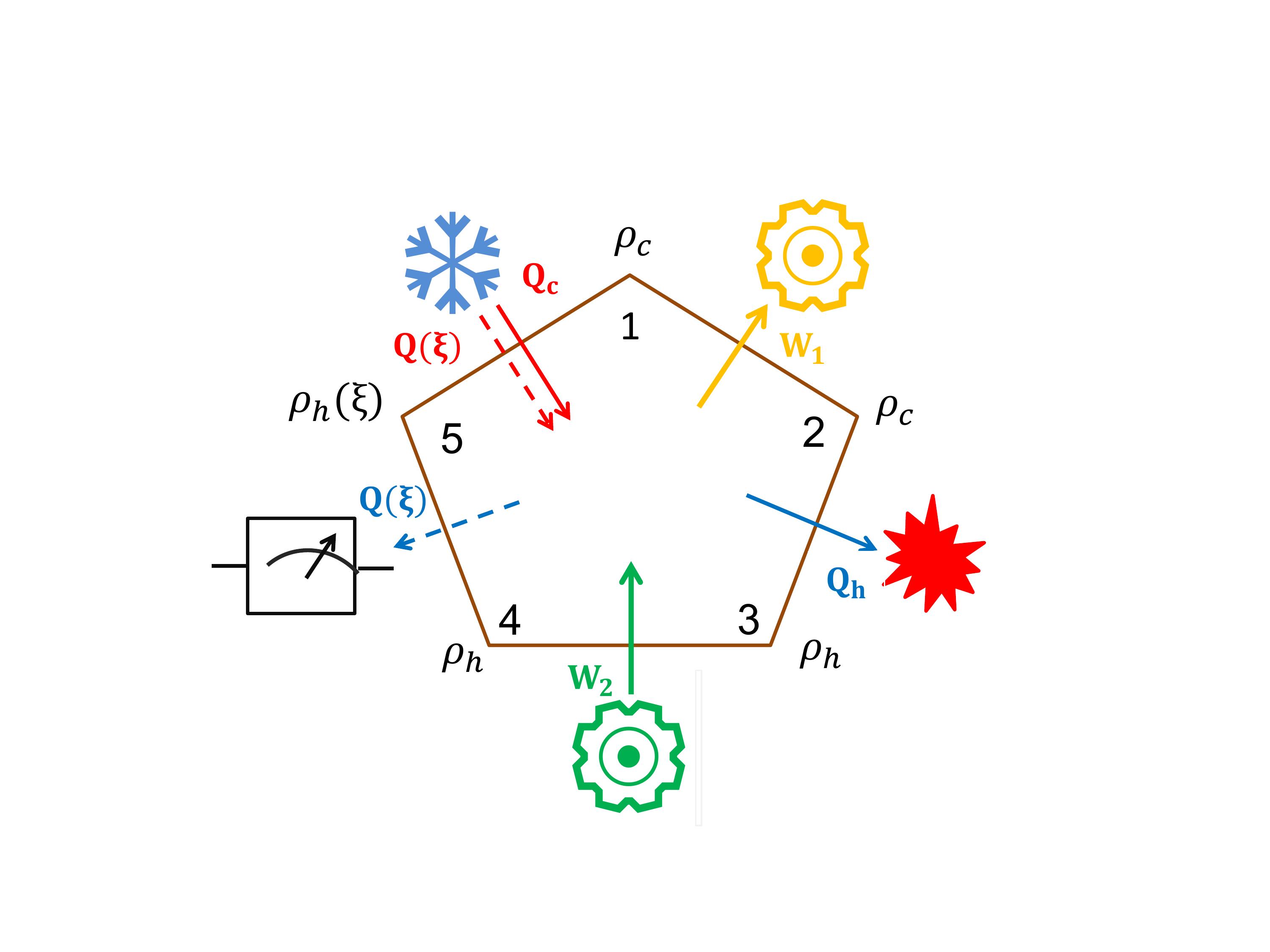
Figure 1:

Fig. 2. The COP for the first type modified Otto cycle refrigerator (Eq. (9)), in terms of measurement strength parameter, for some given invested works (Eq. (11)). The parameters $\omega_{h}=10$, $\omega_{c}=2$ and $\beta_{c}=0.4$ have been fixed. For $\beta_{h}=0.25$, $\beta_{h}=0.19$, $\beta_{h}=0.16$ and $\beta_{h}=0.14$, the invested works are $W_{in}=1.87$, $W_{in}=1.43$, $W_{in}=1.13$ and $W_{in}=0.89$ respectively and the corresponding coefficients of performance are denoted by dotted-dashed black, dashed blue, dotted red and solid green lines respectively.

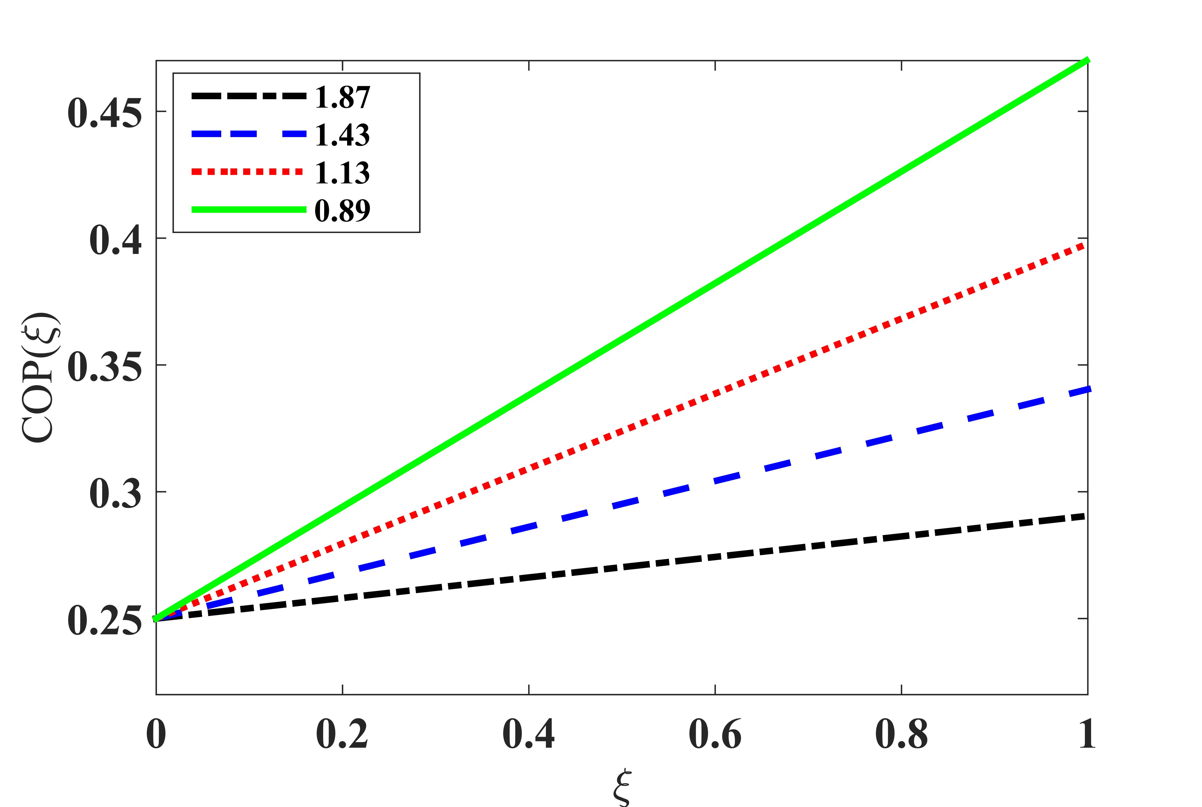
Figure 2:

Fig. 3. The amount of removal heat from the cold reservoir according to Eq. (8), in terms of measurement strength parameter. The solid green line is corresponding to the invested work $W=0.89$ (Eq. (11)), the dotted red line with $W=1.13$, the dashed blue line with $W=1.43$ and the dotted-dashed black line with $W=1.89$. In the strong measurement limit ($\xi\rightarrow 1$), the presence of measurement channel makes to have the most removal of heat from the cold reservoir with the least amount of invested work.

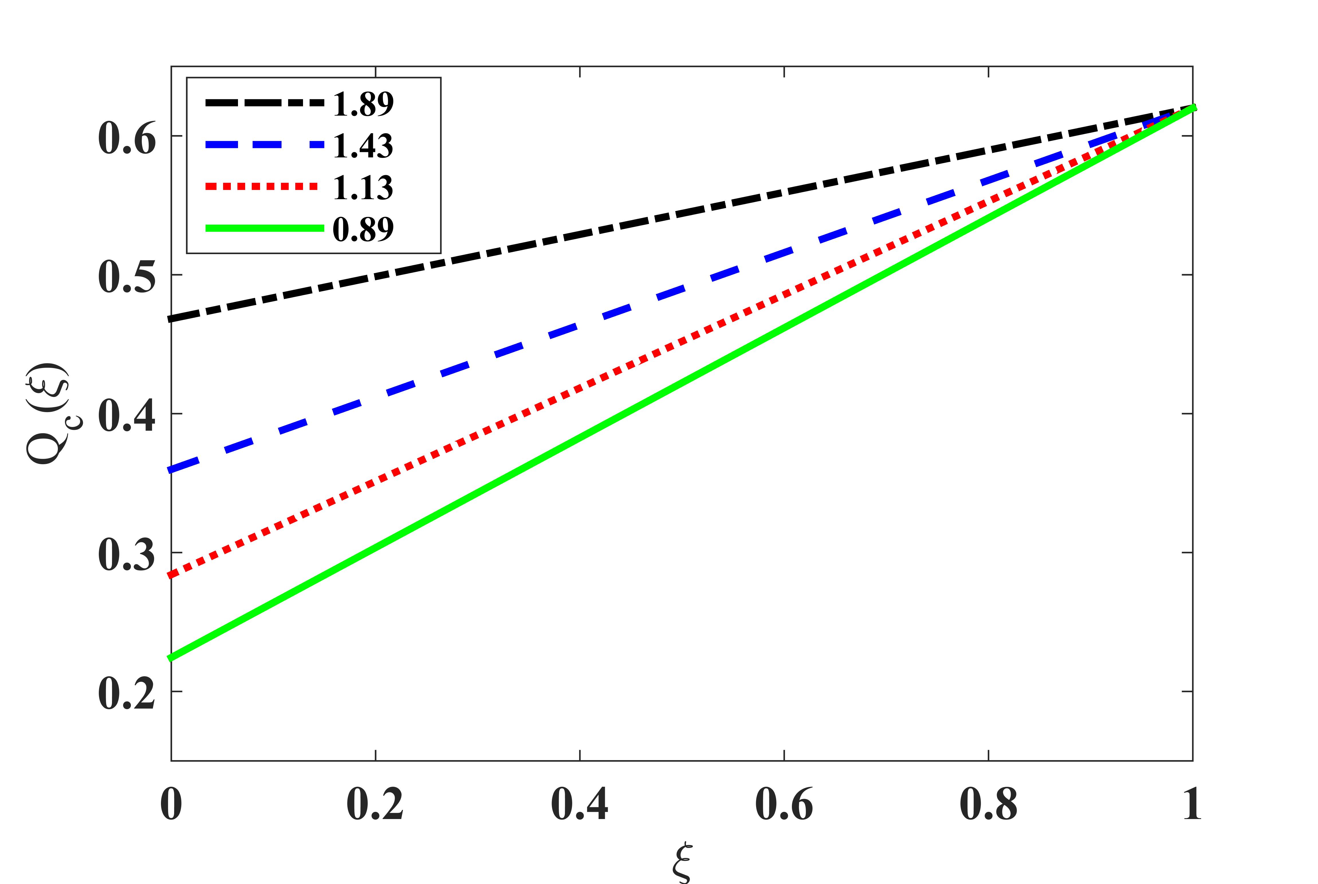
Figure 3:

Fig. 4. Second type modified Otto cycle refrigerator. This five-stroke refrigeration cycle is obtained through inserting the measurement based-stroke after full thermalization of the CM by the cold reservoir in the known Otto cycle. The second type modified Otto cycle, in one hand, provides refrigeration in the same way as the Otto cycle refrigerator, and on the other hand, gives a measurement-induced quantum engine whose efficiency is the same as of the Otto cycle engine. The required work for the refrigeration is $W_{in}=W_{1}+W_{2}$ which causes remove of heat $Q_{c}$ (red solid arrow) from the cold reservoir and flow of heat $Q_{h}$ (blue solid arrow) into the hot reservoir, whereas the solid yellow and green arrows are corresponding to the works $W_{1}$ (extracted) and $W_{2}$ (invested) respectively. The work $W_{in}$ is provided by an external agent, i.e. $W_{ex}(\xi)$, as well as by the measurement-induced engine, i.e. $W(\xi)$ (yellow dashed arrow) through suitable feedback, such that $W_{in}=W_{ex}(\xi)-W(\xi)$. The extracted work from the quantum engine is the consequence of absorption of heat $Q^{\prime}(\xi)$ (red dashed arrow) from the hot reservoir and flow of heat $Q(\xi)$ (blue dashed arrow) into the measurement apparatus. In the limit $\xi\rightarrow\xi_{c}$, $W_{ex}(\xi_{c})=0$, i.e. the modified refrigerator has no need to work supplying by an external agent. In this situation the modified Otto cycle leads to an autonomous refrigerator whose invested work is only provided by the work extracted from the quantum engine such that $W_{in}=-W(\xi_{c})$.

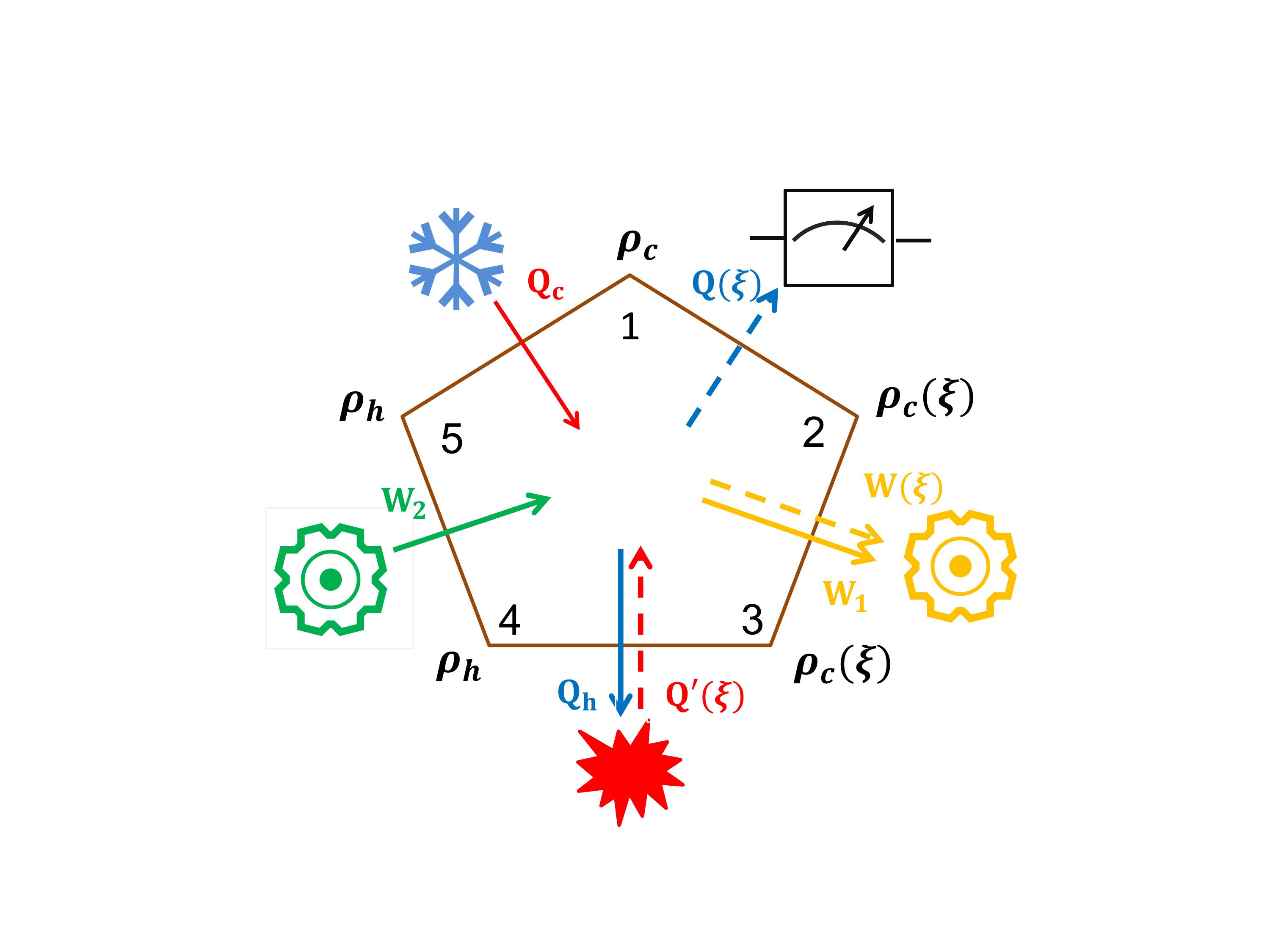
Figure 4:

Fig. 5. First type modified swap refrigerator. (a) At the beginning, each subsystem has been isolated from its own reservoir then the state of bipartite system is $\rho_{h}\otimes\rho_{c}$. (b) The 1st stroke is related to application of swap operator on the bipartite system which makes the cold qubit becomes colder and the hot one becomes hotter. This requires investment of work $W_{in}$ (green solid arrow) on the CM, supplied by an external agent. (c) The effect of measurement process (1), as the 2nd stroke, on the colder qubit causes flow of quantum heat $Q(\xi)$ (blue dashed arrow) from CM into the measurement apparatus. (d) In the 3rd stroke, each subsystem is brought into contact with its own reservoir so the CM absorbs heat $Q_{c}$ and $Q(\xi)$ (red solid and dashed arrows respectively) from the cold reservoir and the heat $Q_{h}$ is flowed from the CM into the hot reservoir.

(a)                   (b)
(c)                   (d)

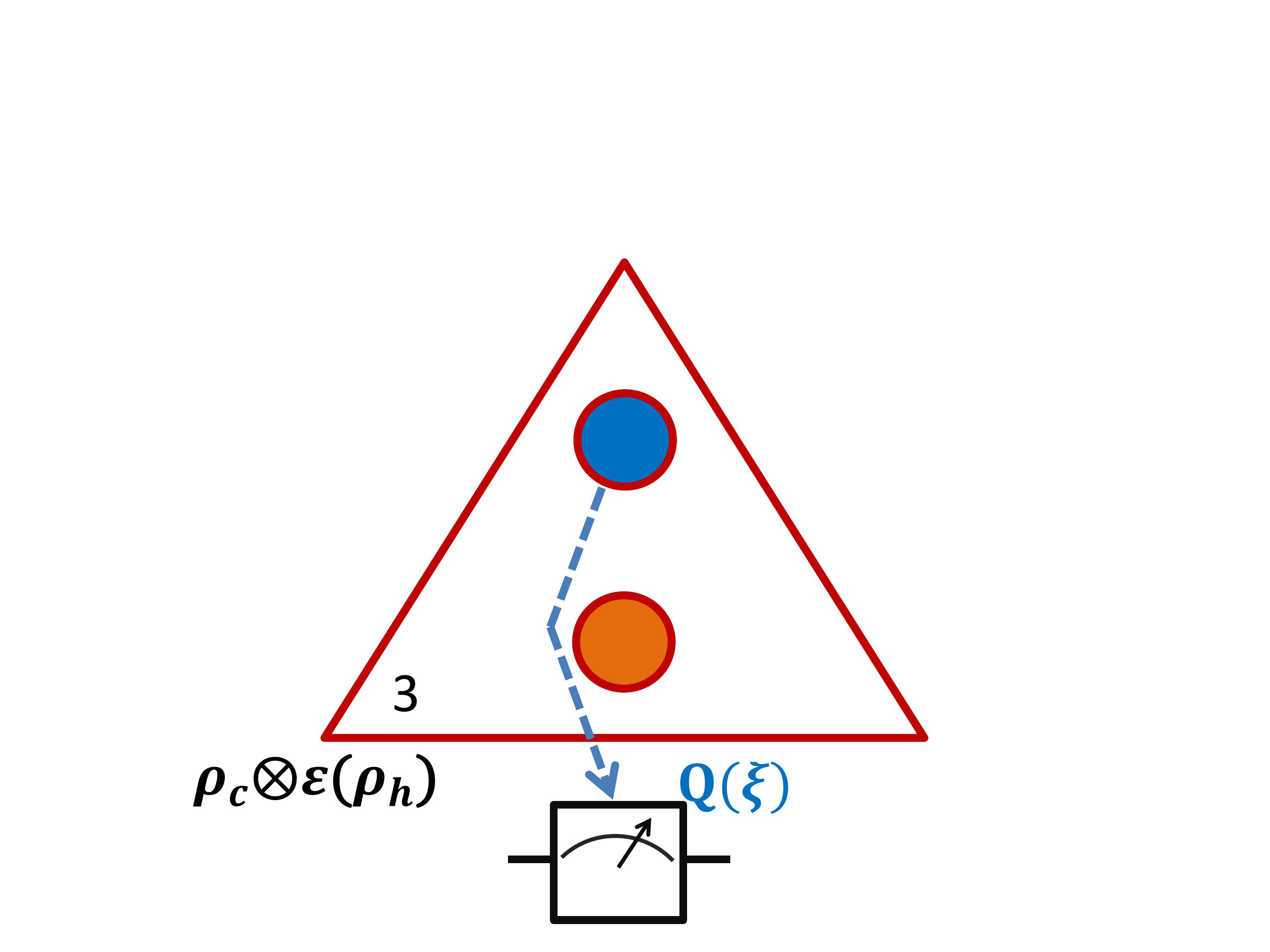
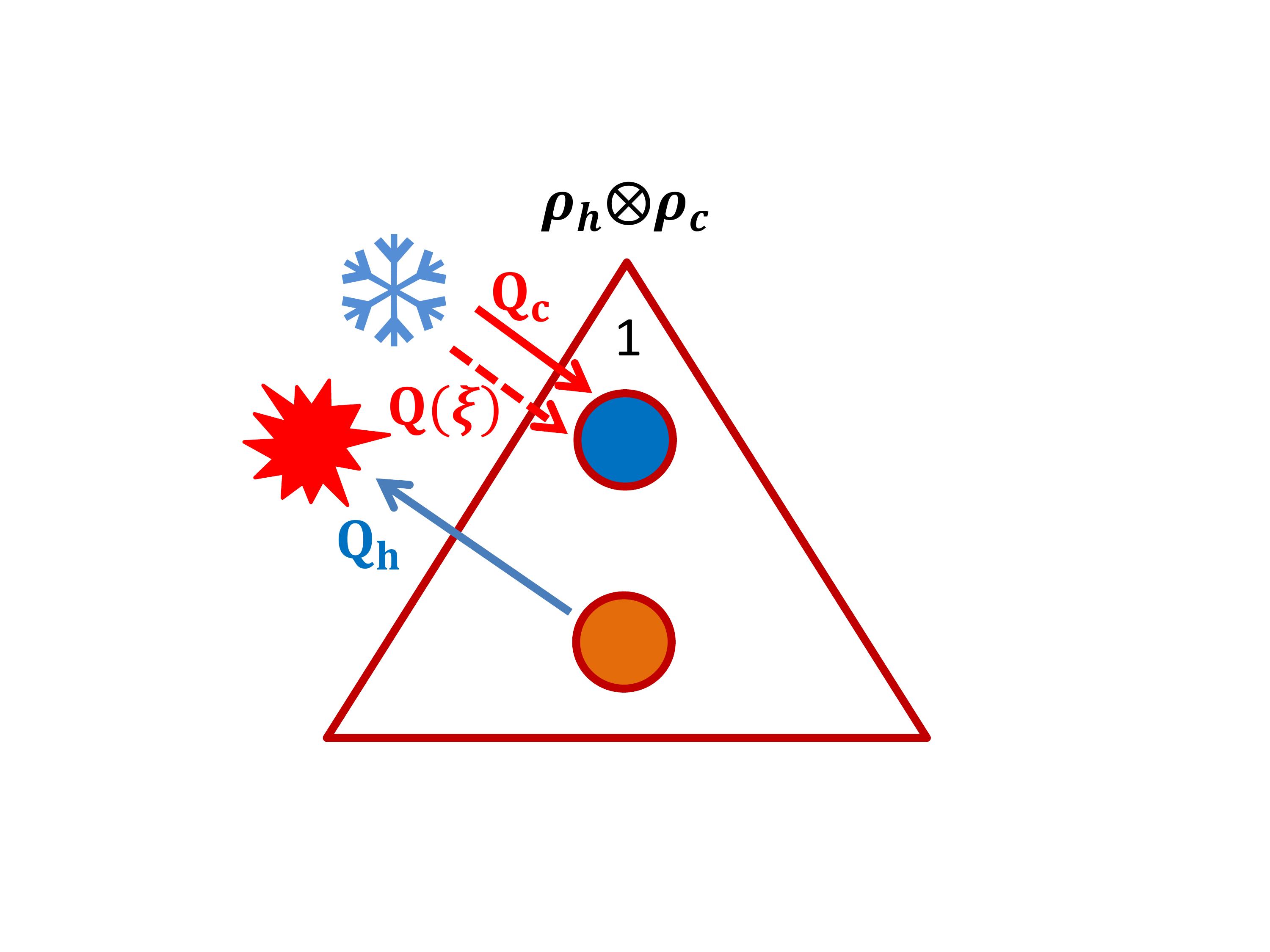
Figure 5:

Fig. 6. Second type modified swap refrigerator. (a) At the beginning, each subsystem has been isolated from its own reservoir so that the state of bipartite system is $\rho_{h}\otimes\rho_{c}$. (b) The subsystem with state $\rho_{c}$ is affected by the generalized measurement defined by (1), so by this (1st) stroke the quantum heat $Q(\xi)$ (blue dashed arrow) is transfered from the mentioned subsystem into the measurement apparatus. (c) The 2nd stroke consists of operation of swap operator which exchanges the subsystems with each other. By this stroke, the required work for the refrigeration, i.e. $W_{in}$ (green solid arrow), is supplied by the measurement-induced quantum engine whose extracted work is $W(\xi)$ (red dashed arrow), as well as by an external agent, i.e. $W_{ex}(\xi)$, such that $W_{in}=W_{ex}(\xi)-W(\xi)$ and $0\leq\xi<\xi_{c}$ (see Eq. (34)). At the end of this stroke, the cold qubit becomes colder and the hot one becomes hotter. (d) The 3rd stroke is provided by bringing the subsystems into contact with their respective reservoirs. During this stroke, the heat $Q_{c}$ (red solid arrow) is transfered from cold reservoir into the CM and the heat $Q_{h}$ (blue solid arrow)is transfered from the CM into the hot reservoir, whereas the heat $Q^{\prime}(\xi)$ (red dashed arrow) is absorbed from the hot reservoir by the CM. Clearly $W_{in}=-(Q_{h}+Q_{c})$ and $W(\xi)=-(Q^{\prime}(\xi)+Q(\xi))$. In the case $\xi=\xi_{c}$, the modified swap provides an autonomous refrigerator where the required work for the refrigeration is only supplied by the quantum engine induced by the measurement channel in the same cycle.

(a)                   (b)
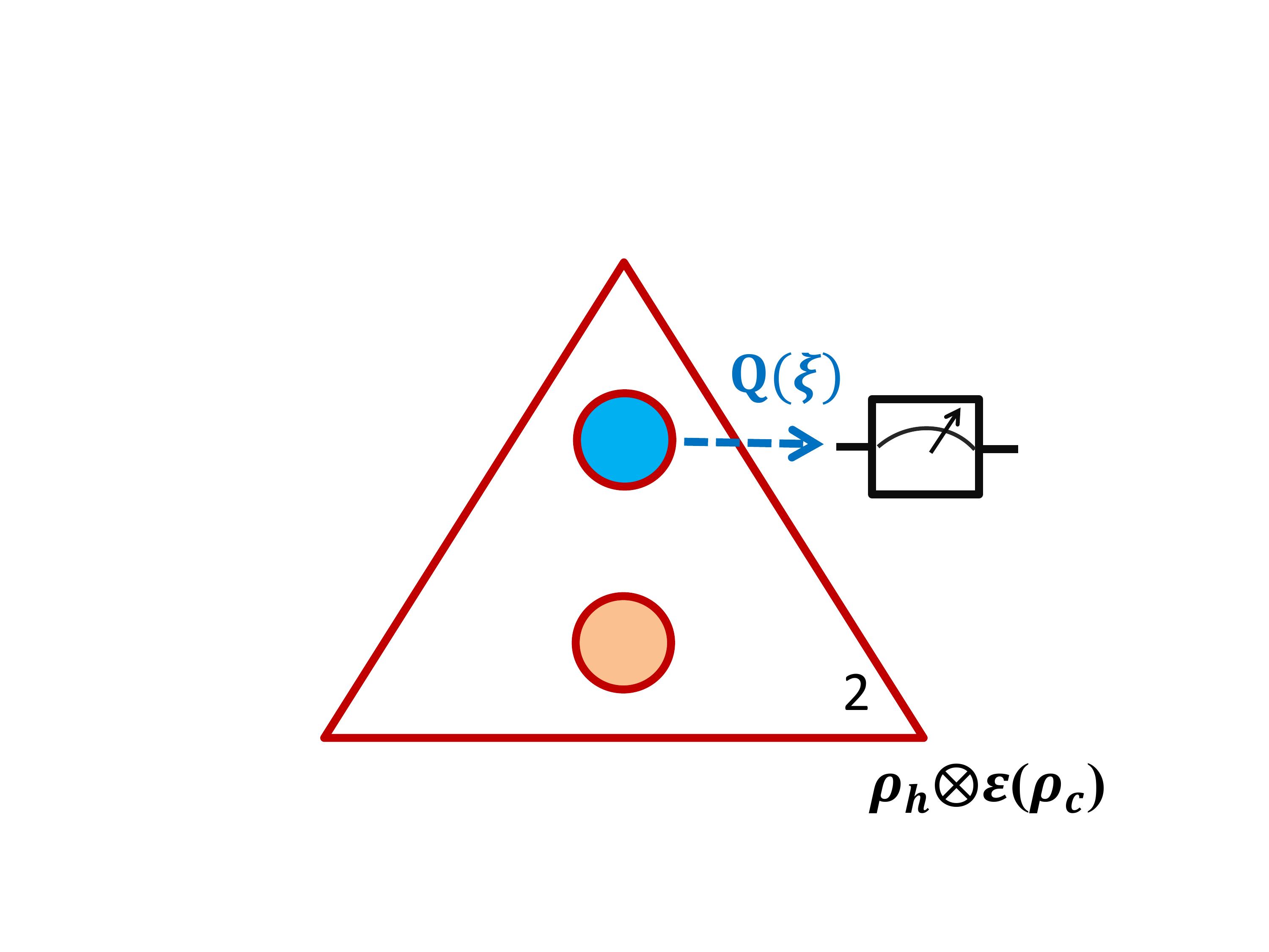
(c)                   (d)

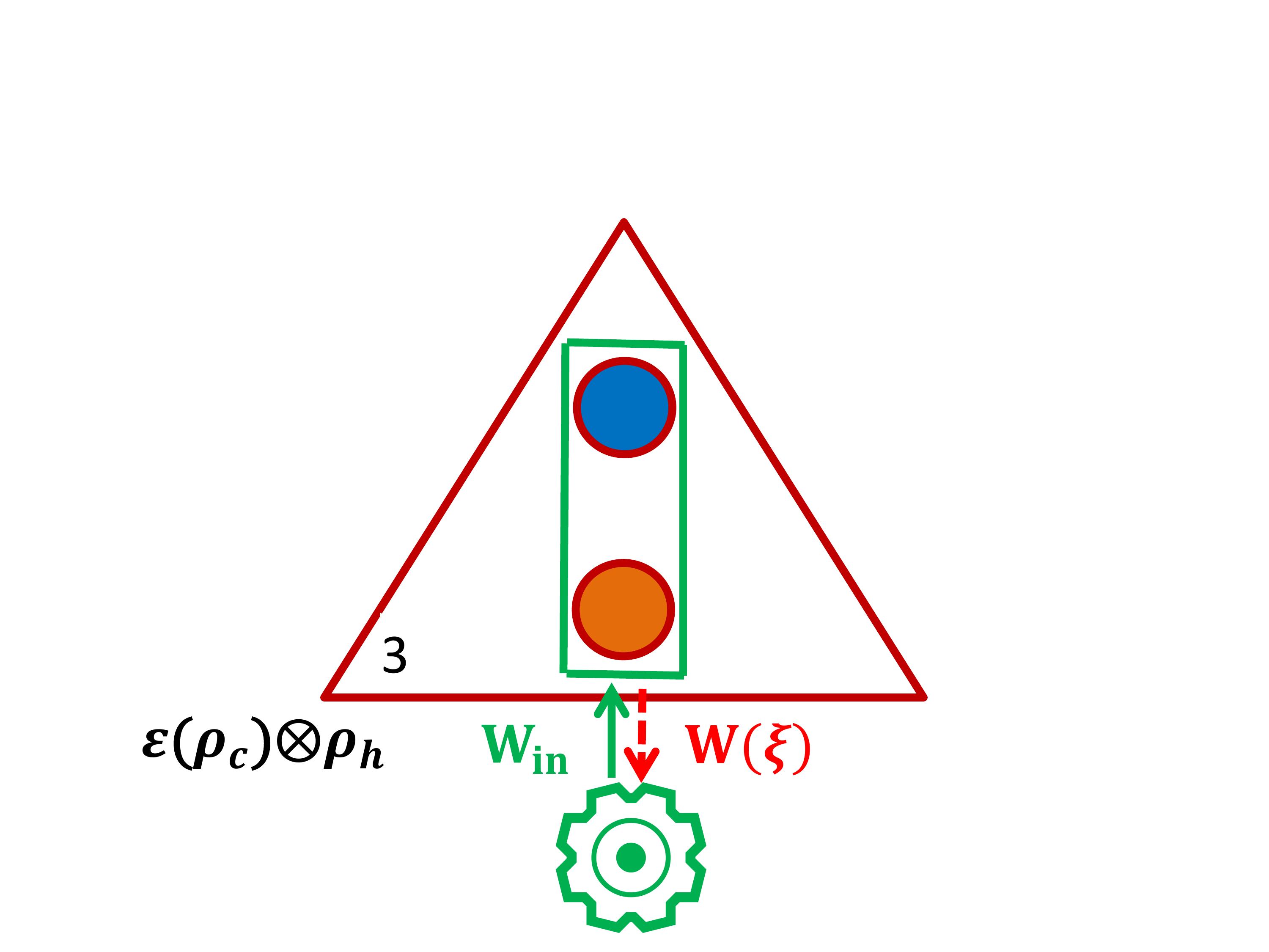
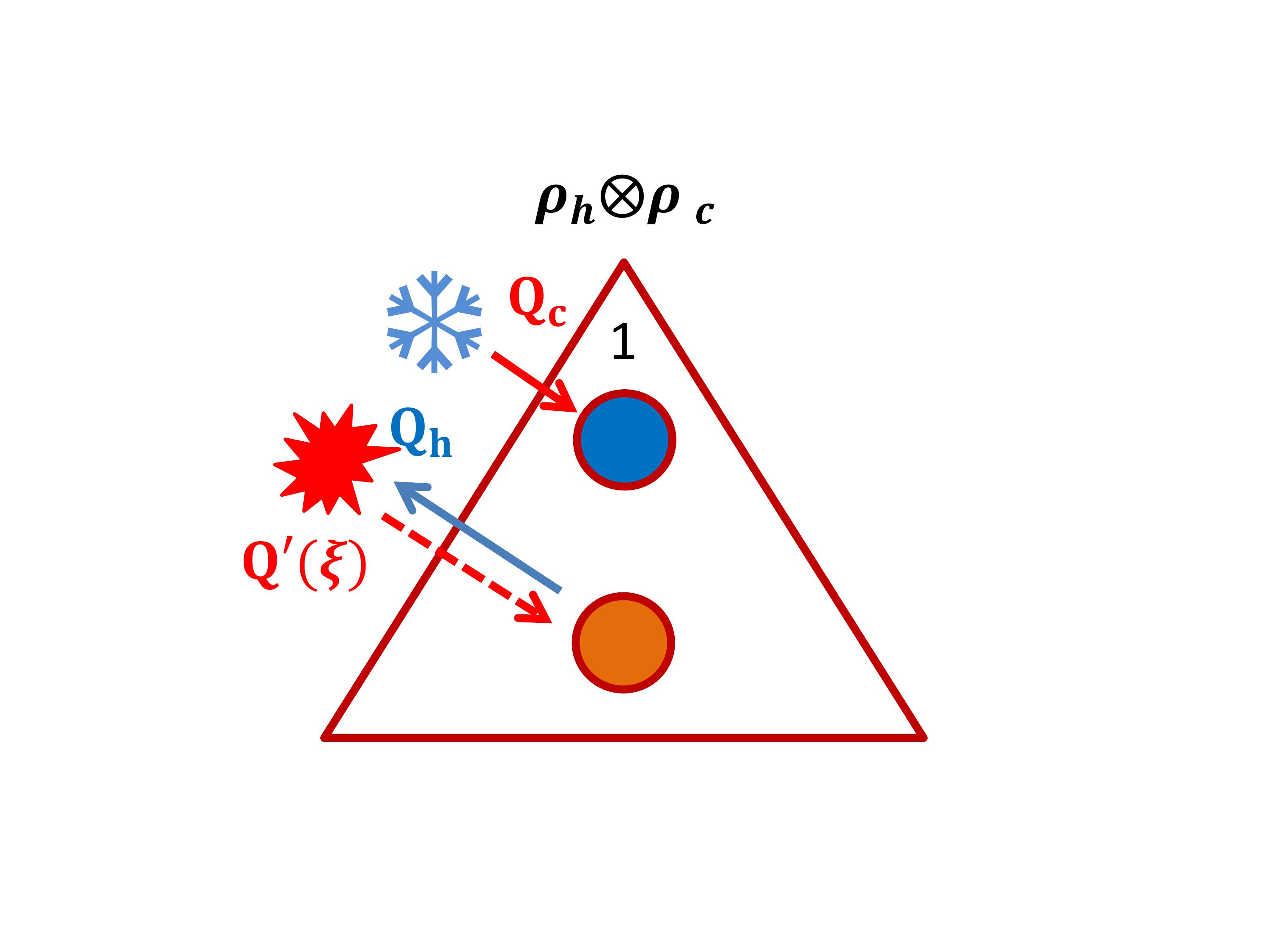
Figure 6:

References

- [1] S. Vinjanampathy and J. Anders, Contemporary Physics 57, 545 (2016)
- [2] J. Goold, M. Huber, A. Riera, L. del Rio and P Skrzypczyk, J. Phys. A: Math. Theor. 49, 143001 (2016)
- [3] F. Binder, L. A. Correa, C. Gogolin, J. Anders, and G. Adesso, Thermodynamics in the quantum Regime: Fundamental aspects and new directions, (Springer, 2019)
- [4] A. N. Jordan, C. Elouard and A. Auffèves, Quantum Stud.: Math. Found. 7, 203 (2020).
- [5] L. Buffoni, A. Solfanelli, P. Verrucchi, A. Cuccoli, and M. Campisi, Phys. Rev. Lett. 122, 070603 (2019)
- [6] K. Brandner, M. Bauer, M. T. Schmid and U. Seifert, New J. Phys. 17 065006 (2015)
- [7] C. Elouard, D. Herrera-Marti, M. Clusel and A. Auffeves, npj Quantum Inf. 3 9 (2017)
- [8] K. Abdelkhalek, Y. Nakata and D. Reeb, arXiv:1609.06981 (2016)
- [9] J. Yi, P. Talkner, and Y. W. Kim, Phys. Rev. E 96, 022108 (2017)
- [10] X. Ding, J. ing, Y. W. Kim, and P. Talkner, Phys. Rev. E 98, 042122 (2018)
- [11] C. Elouard, D. Herrera-Martí, B. Huard, and A. Auffeves, Phys. Rev. Lett. 118, 260603 (2017)
- [12] C. Elouard and A. N. Jordan, Phys. Rev. Lett. 120, 260601 (2018)
- [13] M. H. Mohammady and J. Anders, New J. Phys. 19, 113026 (2017)
- [14] S. K. Manikandan, C. Elouard, K. W. Murch, A. Auffeves, and A. N. Jordan, Phys. Rev. E 105, 044137 (2022).
- [15] N. Behzadi, Quantum engine based on general measurements, J. of Phys. A: Math. Theo. 54, 015304 (2021).
- [16] V. F. Lisboa, P. R. Dieguez, J. R. Guimarães, J. F. G. Santos, and R. M. Serra, Phys. Rev. A 106, 022436 (2022)
- [17] P. R. Dieguez, V. F. Lisboa, and R. M. Serra, Phys. Rev. A 107, 012423 (2023)
- [18] M. T. Mitchison, Contemporary Physics 60, 146 (2019)
- [19] S. K. Manikandan, E. Jussiau, and A. N. Jordan, Phys. Rev. B 102, 235427 (2020)
- [20] G. Maslennikov, S. Ding, R. Hablützel, J. Gan, A. Roulet, S. Nimmrichter, J. Dai, V. Scarani and D. Matsukevich, Nat. Commun. 10, 202 (2019)
- [21] G. Manzano, G-L. Giorgi, R. Fazio, and R. Zambrini, New J. Phys. 21, 123026 (2019)
- [22] P. P. Hofer, M. Perarnau-Llobet, J. B. Brask, R. Silva, M. Huber, and N. Brunner, Phys. Rev. B 94, 235420 (2016)
- [23] R. Silva, G. Manzano, P. Skrzypczyk, and N. Brunner, Phys. Rev. E 94, 032120 (2016)
- [24] L. A. Correa, J. P. Palao, G. Adesso, and D. Alonso, Phys. Rev. E 87, 042131 (2013)
- [25] D. Venturelli, R. Fazio, and V. Giovannetti. Phys. Rev. Lett. 110, 256801 (2013)
- [26] P. Skrzypczyk, N. Brunner, N. Linden and S. Popescu, J. Phys. A: Math. Theor. 44, 492002 (2011)
- [27] A. Levy and R. Kosloff, Phys. Rev. Lett. 108, 070604 (2012)
- [28] A. Mu, B. K. Agarwalla, G. Schaller and D. Segal, New J. Phys. 19, 123034 (2017)
- [29] M. T. Mitchison, M. Huber, J. Prior, M. PWoods, and M. B. Plenio, Quantum Sci. Technol. 1, 015001 (2016)
- [30] K. Jacobs, Quantum Measurements Theory and its Applications, 2014 (Cambridge: Cambridge University Press).
- [31] A. E. Allahverdyan, R. Balian and T. M. Nieuwenhuizen, Europhys. Lett. 67 565 (2004)
- [32] M. Campisi, J. Pekola and R. Fazio, New. J. Phys. 17, 035012 (2015).
- [33] O. Abah and M. Paternostro, Phys. Rev. E 99, 022110 (2019)
- [34] O. Abah and E. Lutz, Phys. Rev. E 98, 032121 (2018)
- [35] G. Jiao, Y. Xiao, J. He, Y. Ma and J. Wang, New J. Phys. 23, 063075 (2021)