In distributive phosphorylation catalytic constants enable non-trivial dynamics

Abstract

Ordered distributive double phosphorylation is a recurrent motif in intracellular signaling and control. It is either sequential (where the site phosphorylated last is dephosphorylated first) or cyclic (where the site phosphorylated first is dephosphorylated first). Sequential distributive double phosphorylation has been extensively studied and an inequality involving only the catalytic constants of kinase and phosphatase is known to be sufficient for multistationarity. As multistationarity is necessary for bistability it has been argued that these constants enable bistability.

Here we show for cyclic distributive double phosphorylation that if its catalytic constants satisfy the very same inequality, then Hopf bifurcations and hence sustained oscillations can occur. Hence we argue that in distributive double phosphorylation (sequential or distributive) the catalytic constants enable non-trivial dynamics.

In fact, if the rate constant values in a network of cyclic distributive double phosphorylation are such that Hopf bifurcations and sustained oscillations can occur, then a network of sequential distributive double phosphorylation with the same rate constant values will show multistationarity – albeit for different values of the total concentrations. For cyclic distributive double phosphorylation we further describe a procedure to generate rate constant values where Hopf bifurcations and hence sustained oscillations can occur. This may, for example, allow for an efficient sampling of oscillatory regions in parameter space.

Our analysis is greatly simplified by the fact that it is possible to reduce the network of cyclic distributive double phosphorylation to what we call a network with a single extreme ray. We summarize key properties of these networks.

Keywords: distributive phosphorylation, extreme vector, Hopf bifurcation, sustained oscillations

1 Introduction

Phosphorylation is a process where proteins are altered by adding and removing phosphate groups at designated binding sites. It is a recurrent motif in many large reaction networks involved in intracellular signaling and control [25]. Often spatial effects are neglected and the time dynamics of the participating chemical species concentrations is described by ordinary differential equations. There exists a plethora of small ODE models that include phosphorylation at one or two binding sites together with the interaction of various regulating chemical species, see, for example, [21]. These models exhibit a wide range of dynamical properties ranging from multistationarity and bistability to sustained oscillations [21].

Phosphorylation and dephosphorylation are catalyzed by two enzymes, a kinase and a phosphatase. As described in [4, 23], this process can either be processive or distributive: if it is processive, then all available binding sites are phosphorylated or de-phosphorylated upon binding of protein and kinase/phosphatase. If the process is distributive, then at most one binding site is modified upon each binding of protein and kinase or phosphatase. Furthermore, multisite phosphorylation and dephosphorylation can occur at a random sequence of binding sites or at an ordered sequence of binding sites. An ordered mechanism is either sequential or cyclic [4, 23]. In a sequential mechanism the last site to be phosphorylated is dephosphorylated first, while in a cyclic mechanism the first site to be phosphorylated is also dephosphorylated first – as depicted in the reaction schemes of Fig. 1.

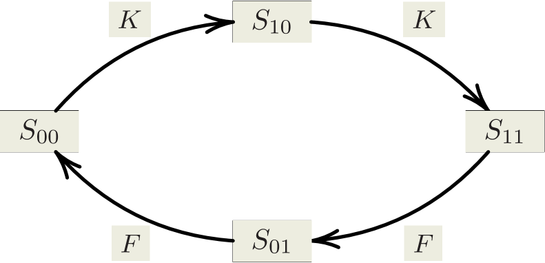
(a) Cyclic & distributive

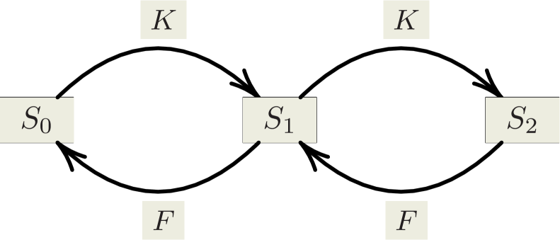
(b) Sequential & distributive

Figure 1: Reaction schemes describing distributive double phosphorylation of a protein $S$ at two binding sites by a kinase $K$ and a phosphatase $F$. Panel (1(a)) cyclic double phosphorylation, panel (1(b)) distributive. In panel  (1(a)) the subscript _ij denotes the state of the phosphorylation sites: $0$ unphosphorylated, $1$ phosphorylated (e.g. $S_{10}$ denotes those molecules of $S$, where the first site is phosphorylated and the second site is unphosphorylated). In panel (1(b)) the subscript _i denotes the number of attached phosphate groups (e.g. $S_{0}$ denotes unphosphorylated protein).

Networks of sequential phosphorylation have been studied extensively and it has been shown that already networks without any form of regulation can exhibit non-trivial dynamics. It is, for example, known that models of sequential and processive phosphorylation and dephosphorylation have a unique, globally attracting steady state [12]. For sequential distributive phosphorylation and dephosphorylation multistationarity and bistability have been established [8, 15, 16]. And for a mixed mechanism of sequential distributive phosphorylation and processive dephosphorylation at two binding sites Hopf bifurcations and sustained oscillations have been described in [24] and [10]. For more information about the dynamics of multisite phosphorylation systems see the review [13] and the references therein.

Networks of cyclic phosphorylation have been studied in [26]. The authors study in particular the following mass action network (1) derived from the reaction scheme of Fig. 1(a) (where the notation is the same as in Fig. 1(a) and $KS_{00}$, $KS_{10}$, $FS_{11}$ and $FS_{01}$ denote enzyme-substrate complexes):

$$\begin{split}S_{00}+K\ce{<=>[\kappa_{1}][\kappa_{2}]}KS_{00}\ce{->[\kappa_{3}]}S_{10}+K\ce{<=>[\kappa_{4}][\kappa_{5}]}KS_{10}\ce{->[\kappa_{6}]}S_{11}+K\\ S_{11}+F\ce{<=>[\kappa_{7}][\kappa_{8}]}FS_{11}\ce{->[\kappa_{9}]}S_{01}+F\ce{<=>[\kappa_{10}][\kappa_{11}]}FS_{01}\ce{->[\kappa_{12}]}S_{00}+F\ .\end{split}$$ (1)

In [26] it is shown that for every admissible positive value of the total concentrations and all positive values of the reaction rate constants there exists a unique positive steady state. The authors furthermore provide parameter values where a Hopf bifurcation occurs (with the total amount of kinase as a bifurcation parameter) and sustained oscillations emerge [26, Fig. 4]. The authors however neither describe how the respective parameter values were found nor do they explain how parameter values leading to oscillations can be found.

Here we study the same network (1) and provide an answer to the latter question. In particular, we show that if the rate constants $\kappa_{3}$, $\kappa_{6}$, $\kappa_{9}$ and $\kappa_{12}$ satisfy the inequality

$$\kappa_{3}\,\kappa_{9}-\kappa_{6}\,\kappa_{12}<0,$$ (2)

then Hopf-bifurcations and sustained oscillations can occur. In enzyme catalysis these constants are known as catalytic constants (cf. the discussion in Section 4 or [9]).

To be more precise, we analyze the following irreversible subnetwork of (1)

$$\begin{split}S_{00}+K\ce{->[\kappa_{1}]}KS_{00}\ce{->[\kappa_{3}]}S_{10}+K\ce{->[\kappa_{4}]}KS_{10}\ce{->[\kappa_{6}]}S_{11}+K\\ S_{11}+F\ce{->[\kappa_{7}]}FS_{11}\ce{->[\kappa_{9}]}S_{01}+F\ce{->[\kappa_{10}]}FS_{01}\ce{->[\kappa_{12}]}S_{00}+F\end{split}$$ (3)

and show that if the values of the catalytic constants $\kappa_{3}$, $\kappa_{6}$, $\kappa_{9}$ and $\kappa_{12}$ satisfy (2), then there exist values for $\kappa_{1}$, $\kappa_{4}$, $\kappa_{7}$, $\kappa_{10}$ and the total concentrations such that the steady state Jacobian of network (3) has a complex-conjugate pair of eigenvalues on the imaginary axis. Furthermore, if this eigenvalue pair crosses the imaginary axis as one of the parameters is varied, then a Hopf bifurcation occurs at this particular steady state (Theorem 3.4). We describe a derivative condition for this crossing and a procedure to find such parameter values. Based on a result by [2], we then argue that if a supercritical Hopf bifurcation occurs in network (3) and a stable limit cycle emerges, then the full network (1) will have a stable limit cycle as well (for appropriately chosen values of $\kappa_{2}$, $\kappa_{5}$, $\kappa_{8}$ and $\kappa_{11}$). This is Theorem 3.9.

Finally, we compare our results for cyclic distributive double phosphorylation with those obtained in [9] for sequential distributive double phosphorylation. In [9] an inequality that is sufficient for multistationarity has been described. Remarkably this inequality involves the catalytic constants in the same way as our inequality (2). As multistationarity is necessary for bistability it is argued in [9] that these rate constants enable bistability in sequential and distributive double phosphorylation. Hence we conclude that in distributive phosphorylation (sequential or cyclic) these constants enable non-trivial dynamics.

The paper is organized as follows: to arrive at our results the ODEs derived from network (1) and (3) are analyzed. For this purpose we recall in Section 2 some well known facts about ODEs defined by reaction networks and introduce a special class of reaction networks that we call networks with a single extreme ray. In this section we also derive conditions for a simple Hopf bifurcation in such networks. In Section 3 we first analyze network (3) and verify these bifurcation conditions in Theorem 3.4. Then we turn to the full network (1) and Theorem 3.9. We also present the procedure to determine rate constant and total concentration values. In Section 4 we discuss inequality (2) in the light of the the results presented in [9]. Appendix A and B contain some of the longer proofs of the results presented in Section 2. Appendix C, D and E contain information to reproduce the numerical results displayed in the figures throughout the paper.

2 Biochemical reaction networks with mass action kinetics

To establish our results we exploit the special structure of the Jacobian of a certain class of reaction networks that we call networks with a single extreme ray. We introduce this class here in full generality. To this end we first consider a general reaction network with $n$ species and $r$ reactions in Section 2.1 and recall the structure of the ODEs defined by such a general network. In Section 2.2 we discuss steady states and formally define networks with a single extreme ray. In Section 2.3 we present a formula for the Jacobian of a general reaction network at steady state. In Section 2.4 we discuss the steady state Jacobian of networks with a single extreme ray. Finally, in Section 2.5 we present conditions for simple Hopf bifurcations in networks of this kind.

2.1 Reaction networks with $n$ species and $r$ reactions

We briefly introduce the relevant notation, for a more detailed discussion we refer to the large body of literature on mass action networks, for example, [7] or [11].

To every chemical species we associate a variable $x_{i}$ denoting its concentration. For network (1) and (3) we use the association as given in Table 1.

$x_{1}$	$x_{2}$	$x_{3}$	$x_{4}$	$x_{5}$	$x_{6}$	$x_{7}$	$x_{8}$	$x_{9}$	$x_{10}$
$K$	$F$	$S_{00}$	$S_{10}$	$S_{01}$	$S_{11}$	$KS_{00}$	$KS_{10}$	$FS_{01}$	$FS_{11}$

Table 1: Species and concentration variables for network (1) and (3).

Consider network (1), nodes like $S_{00}+K$ are called complexes. To every complex we associate a vector $y\in\mathbb{R}^{n}$ representing the stoichiometry of the associated chemical species. The complex $S_{00}+K$ consists of one unit of $S_{00}$ and one unit of $K$, hence, in the ordering of Table 1 the vector $y^{T}=(1,0,1,0,0,0,0,0,0,0)$ represents its stoichiometry. In a similar way one arrives at the ten complex vectors for networks (1) and (3) given in Table 3 of Appendix C.

To every reaction $r^{(l)}$ we associate the difference of the complexes at the tip and the tail of the reaction arrow. For example, to the reaction $S_{00}+K\to S_{00}K$ we associate the vector $r^{(l)}=y^{(2)}-y^{(1)}=(-1,-1,0,1,0,0,0,0,0,0)^{T}$ (using the labeling of complexes given in Table 3 of Appendix C). All reaction vectors $r^{(i)}$ are collected as columns of the stoichiometric matrix $S\in\mathbb{R}^{n\times r}$:

$$S=\left[\begin{array}[]{ccc}r^{(1)}&\dots&r^{(r)}\end{array}\right]\ .$$ (4)

To every reaction $r^{(l)}$ we further associate a reaction rate function $v_{l}(k,x)$ describing the ‘speed’ of the reaction. We consider only mass action kinetics, hence the reaction rate function of reaction $r^{(l)}:y^{(i)}\to y^{(j)}$ is given by the monomial function

$$v_{l}(k,x)=k_{l}\,\prod_{l=1}^{n}x_{l}^{y_{l}^{(i)}}=k_{l}\,x^{y^{(i)}},$$

where $k_{l}$ is a parameter called the rate constant and $x^{y}$ is the customary shorthand notation for the product $\prod_{l=1}^{n}x_{l}^{y_{l}}$ of two $n$-vectors $x$ and $y$.

We collect the vectors at the tail of every reaction as columns of a matrix $Y$ and note that this matrix may contain several copies of the same vector:

$$Y=\left[\begin{array}[]{ccc}y^{(1)}&\dots&y^{(r)}\end{array}\right]$$ (5)

We collect all rate constants in a vector $k^{T}=(k_{1}$, …, $k_{r})$ and the monomials $x^{y^{(i)}}$ in a vector

$$\phi(x)=(x^{y^{(1)}},\ldots,x^{y^{(r)}})^{T}\ ,$$ (6)

where the vectors $y^{(i)}$ reference the columns of the matrix $Y$ defined in  (5). The reaction rate function is then defined using $k$ and $\phi(x)$ as

$$v(k,x)=\operatorname{diag}(k)\,\phi(x)\ .$$ (7)

After an ordering of species and reactions is fixed, every reaction network with mass action kinetics defines a matrix $S$ and a reaction rate function $v(k,x)$ in a unique way. These objects in turn define the following system of ODEs:

$$\dot{x}=Sv(k,x)\ ,$$ (8)

where $\dot{x}$ denotes the vector of derivatives with respect to time. Example are abundant in the literature, see, for example, [7, Section 2] or [11].

Often the matrix $S$ does not have full row rank. In this case let $W$ be a matrix whose columns span $\ker(S^{T})$, that is a full rank matrix $W$ with $W^{T}\,S\equiv 0$. Then $W^{T}\,\dot{x}\equiv 0$ and for every solution $x(t)$ with initial value $x(0)=x_{0}$ one obtains

$$W^{T}\,x(t)=W^{T}\,x_{0}=\text{const. }$$

Hence, if $\operatorname{rank}(S)=s<n$, then one obtains $n-s$ conservation relations

$$W^{T}\,x=c\ .$$ (9)

2.2 Steady states

We are interested in points ($k$,$x$) that are solutions of

$$Sv(k,x)=0\ .$$ (10)

If ($k$,$x$) is a solution of (10), then $x$ is a steady state of (8) for the rate constants $k$.

We proceed as in [6] and express the reaction rates $v(k,x)$ at a steady state as a nonnegative combination of the extreme vectors of the pointed polyhedral cone $\ker(S)\cap\mathbb{R}_{\geq 0}^{r}$. This idea goes back to Clarke and coworkers (cf. for example, [5, 13]) and it is as follows: ($k$,$x$) satisfy (10), if and only if the corresponding $v(k,x)$ is such that $v(k,x)\in\ker(S)\cap\mathbb{R}_{\geq 0}^{r}$ (cf. eg. [6]).

Convex polyhedral cones have a finite number of extreme vectors (up to a scalar positive multiplication [22]). Therefore, any element $v$ of such a cone can be represented as a nonnegative linear combination of its extreme vectors $\{E_{1},\ldots,E_{l}\}$

$$v=\sum_{i=1}^{l}\lambda_{i}E_{i}=E\lambda,\;\lambda\in\mathbb{R}_{\geq 0}^{l},$$ (11)

where $E$ is the matrix with columns $E_{1},\dots,E_{l}$ and $\lambda^{T}=(\lambda_{1},\dots,\lambda_{l})$.

Remark 2.1 (The relative interior of $\ker(S)\cap\mathbb{R}_{\geq 0}^{r}$).

1. As explained in, for example, [27], a system (8) has positive solutions ($k$,$x$), if and only if the matrix $E$ does not contain a zero row. Hence we will only consider networks where the matrix $E$ are of this kind.

2. We are only interested in positive values of $k$ and $x$. Thus we are only interested in $v(k,x)$ that are strictly positive and hence belong to the relative interior of the cone $\ker(S)\cap\mathbb{R}_{\geq 0}^{r}$. Consequently we are only interested in those $\lambda\in\mathbb{R}_{\geq 0}^{l}$ that yield a positive $E\lambda$. In the remainder of the paper we therefore restrict $\lambda\in\mathbb{R}_{\geq 0}^{l}$ to the set:

   $$\Lambda(E):=\left\{\lambda\in\mathbb{R}_{\geq 0}^{l}|E\lambda>0\right\}\ .$$ (12)

   This set has been introduced in [7], cf. [7, Remark 4].

3. A more detailed discussion of the relation between positive solutions of (10), the cone $\ker(S)\cap\mathbb{R}_{\geq 0}^{r}$ and the generator matrix $E$ can be found in [27], cf. in particular [27, Proposition 6].

In the analysis of network (1) we will later analyze subnetworks that fit the following definition:

Definition 1 (Networks with a single extreme ray).

Consider a reaction network with stoichiometric matrix $S$. If the cone $\ker(S)\cap\mathbb{R}_{\geq 0}^{r}$ is generated by a single positive vector then we call it a network with a single extreme ray.

As discussed in Remark 2.1, if $x>0$ and $k>0$, then $v(k,x)=\operatorname{diag}(k)\phi(x)>0$. Consequently, if ($k$,$x$) satisfy the steady state equation (10), then $v(k,x)\in\ker(S)\cap\mathbb{R}_{\geq 0}^{r}$ and there exists a vector $\lambda\in\Lambda\left(E\right)$, such that (11) is satisfied. Thus one may parameterize all reaction rates at steady states via the equation

$$\operatorname{diag}(k)\,\phi(x)=E\,\lambda,\;\lambda\in\Lambda\left(E\right)\ .$$ (13)

Likewise, given some $\lambda\in\Lambda\left(E\right)$ and a positive $x$ one obtains a positive vector $k$ such that ($k$,$x$) satisfy the steady state equation (10) by the following formula:

$$k=\operatorname{diag}(\phi(h))E\lambda,$$ (14)

where

$$h=\frac{1}{x}\;.$$ (15)

We observe that (i) the formula (15) is well defined as by assumption $x>0$, (ii) that the vector $k$ from (14) is positive since all entries of $E\lambda$ are positive (as, by assumption, the matrix $E$ does not have any zero rows, cf. Remark 2.1) and (iii) that the formula (14) is obtained by solving the $k$-linear equation (13) for $k$.

2.3 The Jacobian at steady state

The equations (11) & (13) introduce a parametrization of the reaction rates $v(k,x)$ at steady states in terms of the convex parameters $h$ and $\lambda$. This parameterization can be used to parameterize the Jacobian at steady state: as explained in detail in [6] or [5], if ($k$,$x$) satisfy the steady state equation (10) and hence $v(k,x)$ is such that (13) holds, then the Jacobian evaluated at that ($k$, $x$) is given by the following formula (cf.[6, Proposition 2]):

$$J(k,x)=J(h,\lambda)=N\operatorname{diag}(E\lambda)Y^{T}\operatorname{diag}(h),$$ (16)

where $Y$ denotes the matrix introduced in (5).

2.4 The Jacobian of networks with a single extreme vector

For any reaction network where the cone $\ker(S)\cap\mathbb{R}_{\geq 0}^{r}$ is spanned by a single positive vector $E$ the parameter $\lambda$ is a positive scalar and formula (16) is equivalent to

$$J_{\lambda}(h)=\lambda S\operatorname{diag}(E)Y^{T}\operatorname{diag}(h)\ .$$ (17)

We use $J_{\lambda}(h)$ to denote the Jacobian in this special case.

Here we comment on the characteristic polynomial of general matrices $J_{\lambda}(h)$, that is on the polynomial $\det(\mu I-J_{\lambda}(h))$ of an $n\times n$ Jacobian of the form (17). We will assume that $\operatorname{rank}(J_{\lambda})=s\leq n$ and we will use the symbol $a_{i}(h,\lambda)$ to denote the coefficients of its characteristic polynomial. We will also discuss the case $\lambda=1$, that is, the characteristic polynomial $\det(\mu I-J_{1}(h))$ of $J_{1}(h)$ with coefficients $b_{i}(h)$. For this purpose, the characteristic polynomial of the Jacobian $J_{\lambda}(h)$ is denoted by

$$\det(\mu I-J_{\lambda}(h))=\mu^{n-s}(\mu^{s}+a_{1}(\lambda,h)\mu^{s-1}+\ldots+a_{s}(\lambda,h)),$$ (18)

while the characteristic polynomial of $J_{1}(h)$ is denoted by

$$\det(\mu I-J_{1}(h))=\mu^{n-s}(\mu^{s}+b_{1}(h)\mu^{s-1}+\ldots+b_{s}(h))\;.$$ (19)

Concerning these polynomials we have the following corollary of Lemma A.4 in Appendix A where we show the relationship between the coefficients $a_{i}(h,\lambda)$ and $b_{i}(h)$.

Corollary 2.2.

Suppose the matrix $E$ consists of a single positive column vector. Let $J_{\lambda}(h)$ be as in (17) with $\operatorname{rank}(J_{\lambda}(h))=\operatorname{rank}(J_{1}(h))=s<n$ and let $a_{i}(\lambda,h)$, $b_{i}(h)$ be the coefficients of the characteristic polynomials in (18) and in (19). Then the coefficients $a_{i}(\lambda,h)$ and $b_{i}(h)$ satisfy:

$$a_{i}(\lambda,h)=\lambda^{i}b_{i}(h),\,i=1,\,\ldots,\,s\ .$$ (20)

Moreover, the polynomial $\det(\mu I-J_{\lambda}(h))$ is given by the following formula:

$$\begin{split}\det(\mu I_{n}-J_{\lambda}(h))&=\det(\mu I_{n}-\lambda J_{1}(h))\\ &=\mu^{n-s}\lambda^{s}\left(\left(\frac{\mu}{\lambda}\right)^{s}+\sum_{i=1}^{s}b_{i}(h)\left(\frac{\mu}{\lambda}\right)^{s-i}\right)\end{split}$$ (21)

We observe the following consequences of Corollary 2.2:

Remark 2.3.

1. By (21) it follows that if $\omega(h)$ is an eigenvalue of $J_{1}(h)$, then $\mu(\lambda,\omega)=\lambda\omega(h)$ is an eigenvalue of $J_{\lambda}(h)$.

2. In our setting $\lambda>0$, hence the sign of the real part of the eigenvalues $Re(\mu(\lambda,h))$ of $J_{\lambda}(h)$ is independent of $\lambda$: $\operatorname{sign}(Re(\mu(\lambda,h)))=\operatorname{sign}(Re(\omega(h)))$.

3. In particular, the matrix $J_{\lambda}(h)$ has a purely imaginary pair of eigenvalues $\pm i\lambda\omega(h)$ if and only if $J_{1}(h)$ has a purely imaginary pair $\pm i\omega(h)$.

2.5 Simple Hopf bifurcations in networks with a single extreme ray

We recall the definition of a simple Hopf bifurcation for a parameter dependent system of ODEs of the form $\dot{x}=g_{p}(x)$, where $x\in\mathbb{R}^{s}$, and $g_{p}(x)$ varies smoothly in $p$ and $x$. Let $x^{*}\in\mathbb{R}^{s}$ be a steady state of the ODE system for some fixed value $p_{0}$, that is, $g_{p_{0}}(x^{*})=0$. Furthermore, we assume that we have a smooth curve of steady states around $p_{0}$:

$$p~{}\mapsto~{}x(p)~{}\text{with $x(p_{0})=x^{*}$.}$$

That is, $g_{p}\left(x(p)\right)=0$ for all $p$ close enough to $p_{0}$.

Further let $J(x(p),p)$ be the Jacobian of $g_{p}(x)$ evaluated at $x(p)$. If, as $p$ varies, a complex-conjugate pair of eigenvalues of $J(x(p),p)$ crosses the imaginary axis, then there exists a Hopf bifurcation at $(x(p_{0},p_{0}))$. A simple Hopf bifurcation occurs at $(x(p_{0}),p_{0})$, if no other eigenvalue crosses the imaginary axis at the same value $p_{0}$. In this case, a limit cycle arises. If the Hopf bifurcation is supercritical, then stable periodic solutions are generated for nearby parameter values [19].

Similar to [10] and [6] we want to build on results described in [19] and [28] to establish Hopf bifurcations. As in previous work (cf. e.g. [6, 19, 28]), we will use a criterion based on the following Hurwitz determinants:

Definition 2.

The $i$-th Hurwitz matrix of a univariate polynomial $p(z)=a_{0}z^{s}+a_{1}z^{s-1}+\cdots+a_{s}$ is the following $i\times i$ matrix:

$$H_{i}~{}=~{}\begin{pmatrix}a_{1}&a_{0}&0&0&0&\cdots&0\\ a_{3}&a_{2}&a_{1}&a_{0}&0&\cdots&0\\ \vdots&\vdots&\vdots&\vdots&\vdots&&\vdots\\ a_{2i-1}&a_{2i-2}&a_{2i-3}&a_{2i-4}&a_{2i-5}&\cdots&a_{i}\end{pmatrix}~{},$$

in which the $(k,l)$-th entry is $a_{2k-l}$ as long as $0\leq 2k-l\leq s$, and $0$ otherwise. The determinants $\det(H_{i})$ are called Hurwitz determinants.

To every square matrix one can associate Hurwitz matrices via its characteristic polynomial in an analogous way. In the following we consider two families of Hurwitz matrices constructed according to Definition 2: matrices $H_{l}(\lambda,h)$ obtained from coefficients $a_{i}(\lambda,h)$ of (18) and matrices $G_{l}(h)$ of coefficients $b_{i}(h)$ of (19). Our analysis is greatly simplified by the relationship between the two families established in Proposition 2.4 below (a proof is given in Appendix B):

Proposition 2.4.

The Hurwitz determinants for the characteristic polynomials (18) and (19) satisfy the following equation

$$\det\left(H_{l}(\lambda,h)\right)=\lambda^{l(l+1)/2}\det\left(G_{l}(h)\right),\;\;l=1,2,\ldots,s\;.$$

The following proposition is a specialization of [6, Proposition 1] and [28, Theorem 2] to a network where $\ker(S)\cap\mathbb{R}_{\geq 0}^{r}$ is generated by a single positive vector. It implies that for such networks to detect a simple Hopf bifurcation one only needs to study the polynomial (19) and its Hurwitz matrices $G_{i}$, $i=1,2,\ldots,s$.

Proposition 2.5.

Let $\dot{x}=Sv(k,x)$ be an ODE system model for a reaction network with mass action kinetics where $\operatorname{rank}(S)=s$. Suppose that the matrix $E$ in (11) consists of a single positive vector and let $J_{\lambda}(h)$ be the corresponding Jacobian in convex parameters. Further let the characteristic polynomials of $J_{\lambda}(h)$ and $J_{1}(h)$ be as in (18) and (19), respectively. If there exists a fixed value $h=h^{*}$ such that

$$\begin{split}b_{s}(h^{*})&>0\text{ and}\\ \det(G_{1}(h^{*}))&>0,\;\ldots,\;\det(G_{s-2}(h^{*}))>0\text{ and}\\ \det(G_{s-1}(h^{*}))&=0\ ,\end{split}$$ (22)

then

1. $J_{1}(h^{*})$ has a single pair of purely imaginary eigenvalues,

2. $J_{\lambda}(h^{*})$ has a single pair of purely imaginary eigenvalues for all $\lambda>0$,

3. for the dynamical system $\dot{x}=Sv(k,x)$ there exists a simple Hopf bifurcation at $h=h^{*}$ for all $\lambda>0$ if there exists some $l\in\{1,2,\ldots,n\}$ such that

   $$\frac{\partial\det(G_{n-1})}{\partial h_{l}}|_{h_{l}=h_{l}^{*}}\neq 0\ .$$ (23)

Proof.

1. The proof follows by [6, Proposition 1].

2. By Corollary 2.2 $\operatorname{sign}(b_{s}(h^{*}))=\operatorname{sign}(a_{s}(h^{*},\lambda))$ for all $\lambda>0$. Likewise, by Proposition 2.4 $\operatorname{sign}(\det(G_{l}(h^{*})))=\operatorname{sign}(\det(H_{l}(h^{*},\lambda)))$, $l=1$, …, $s$ for all $\lambda>0$. Hence by (a) and by [6, Proposition 1] the Jacobian $J_{\lambda}(h^{*})$ has a single pair of purely imaginary eigenvalues for all $\lambda>0$.

3. The fact that $J_{\lambda}(h_{l}^{*})$ for all $\lambda>0$ has a single pair of purely imaginary eigenvalues has been established in (b). Proposition 2.4 implies the following relationship between the two derivatives of $\det\left(H_{s-1}(h,\lambda)\right)$ and $\det\left(G_{s-1}(h,\lambda)\right)$ with respect to the $h_{l}$:

   $$\frac{\partial\det(H_{s-1}(h,\lambda))}{\partial h_{l}}=\lambda^{\frac{s(s+1)}{2}}\frac{\partial\det(G_{s-1}(h))}{\partial h_{l}},\,l=1,\ldots,n\ .$$

   Thus, if (23) holds for some $l\in\{1$, …, $n\}$, then, for the same $l$, one has

   $$\frac{\partial\det(H_{s-1}(h,\lambda))}{\partial h_{l}}|_{(h^{*},\lambda)}\neq 0\text{ for all $\lambda>0$.}$$

   Therefore, by (a), (b) and by [28, Theorem 2&Remark 2], (c) follows as well.

∎

Remark 2.6.

The parameter $\lambda$ is not suited as a bifurcation parameter in (23) as by Proposition 2.4 $\det(H_{s-1}(h,\lambda))=\lambda^{\frac{s(s-1)}{2}}\det(G_{s-1}(h))$. Hence $\frac{\partial\det(H_{s-1}(h,\lambda))}{\partial\lambda}|_{h=h^{*}}=0$, whenever $\det(G_{s-1}(h^{*}))=0$ (cf. Remark 2.3 explaining that the existence of a pair of purely imaginary eigenvalues is independent of $\lambda$).

3 Analysis of networks of cyclic distributive double phosphorylation

To derive a dynamical model of network (1) we assign the variables given in Table 1 to the chemical species and obtain the following ODEs:

$$\dot{x}_{1} =-\kappa_{1}x_{1}x_{3}-\kappa_{4}x_{1}x_{4}+(\kappa_{2}+\kappa_{3})x_{7}+(\kappa_{5}+\kappa_{6})x_{8}$$ (24a)

$$\dot{x}_{2} =-\kappa_{10}x_{2}x_{5}-\kappa_{7}x_{2}x_{6}+(\kappa_{8}+\kappa_{9})x_{10}+(\kappa_{11}+\kappa_{12})x_{9}$$ (24b)

$$\dot{x}_{3} =-\kappa_{1}x_{1}x_{3}+\kappa_{2}x_{7}+\kappa_{12}x_{9}$$ (24c)

$$\dot{x}_{4} =-\kappa_{4}x_{1}x_{4}+\kappa_{3}x_{7}+\kappa_{5}x_{8}$$ (24d)

$$\dot{x}_{5} =-\kappa_{10}x_{2}x_{5}+\kappa_{9}x_{10}+\kappa_{11}x_{9}$$ (24e)

$$\dot{x}_{6} =-\kappa_{7}x_{2}x_{6}+\kappa_{8}x_{10}+\kappa_{6}x_{8}$$ (24f)

$$\dot{x}_{7} =-(\kappa_{2}+\kappa_{3})x_{7}+\kappa_{1}x_{1}x_{3}$$ (24g)

$$\dot{x}_{8} =-(\kappa_{5}+\kappa_{6})x_{8}+\kappa_{4}x_{1}x_{4}$$ (24h)

$$\dot{x}_{9} =-(\kappa_{11}+\kappa_{12})x_{9}+\kappa_{10}x_{2}x_{5}$$ (24i)

$$\dot{x}_{10} =-(\kappa_{8}+\kappa_{9})x_{10}+\kappa_{7}x_{2}x_{6}$$ (24j)

Using the same variables $x_{1}$, …, $x_{10}$ as in Table 1, we obtain the following ODEs:

$$\dot{x}_{1} =-\kappa_{1}x_{1}x_{3}-\kappa_{4}x_{1}x_{4}+\kappa_{3}x_{7}+\kappa_{6}x_{8},$$ (25a)

$$\dot{x}_{2} =\phantom{-}\kappa_{9}x_{10}-\kappa_{10}x_{2}x_{5}-\kappa_{7}x_{2}x_{6}+\kappa_{12}x_{9},$$ (25b)

$$\dot{x}_{3} =-\kappa_{1}x_{1}x_{3}+\kappa_{12}x_{9},$$ (25c)

$$\dot{x}_{4} =-\kappa_{4}x_{1}x_{4}+\kappa_{3}x_{7},$$ (25d)

$$\dot{x}_{5} =\phantom{-}\kappa_{9}x_{10}-\kappa_{10}x_{2}x_{5},$$ (25e)

$$\dot{x}_{6} =-\kappa_{7}x_{2}x_{6}+\kappa_{6}x_{8},$$ (25f)

$$\dot{x}_{7} =\phantom{-}\kappa_{1}x_{1}x_{3}-\kappa_{3}x_{7},$$ (25g)

$$\dot{x}_{8} =\phantom{-}\kappa_{4}x_{1}x_{4}-\kappa_{6}x_{8},$$ (25h)

$$\dot{x}_{9} =\phantom{-}\kappa_{10}x_{2}x_{5}-\kappa_{12}x_{9},$$ (25i)

$$\dot{x}_{10} =-\kappa_{9}x_{10}+\kappa_{7}x_{2}x_{6}\ .$$ (25j)

Both networks have the same set of three conservation relations, one for the total amount of kinase ($c_{1}$), phosphatase ($c_{2}$), and substrate ($c_{3}$), respectively:

$$x_{1}+x_{7}+x_{8\phantom{0}} =c_{1}$$

$$x_{2}+x_{9}+x_{10} =c_{2}$$ (26)

$$x_{3}+x_{4}+x_{5}+x_{6}+x_{7}+x_{8}+x_{9}+x_{10} =c_{3}$$

3.1 Steady states of network (3)

For the network (3) the matrix $E$ consists of a single vector of all 1:

$$E^{T}=(1,1,1,1,1,1,1,1),$$ (27)

hence network (3) is a network with a single extreme ray and we can apply the results of Section 2.4 and 2.5.

Given $E$ from (27) condition (13) consequently becomes (cf. eq. (49) of Appendix C for $v(k,x)$):

$$\kappa_{1}x_{1}x_{3}=\kappa_{3}x_{7}=\kappa_{4}x_{1}x_{4}=\kappa_{6}x_{8}=\kappa_{7}x_{2}x_{6}=\kappa_{9}x_{10}=\kappa_{10}x_{2}x_{5}=\kappa_{12}x_{9}=\lambda\ .$$

These equations can be solved for $x$ (in terms of $k$ and $\lambda$) to obtain the following steady state parameterization:

$$\begin{split}x_{3}&=\frac{\lambda}{\kappa_{1}x_{1}},\,x_{4}=\frac{\lambda}{\kappa_{4}x_{1}},\,x_{5}=\frac{\lambda}{\kappa_{10}x_{2}},\,x_{6}=\frac{\lambda}{\kappa_{7}x_{2}},\\ x_{7}&=\frac{\lambda}{\kappa_{3}},\,x_{8}=\frac{\lambda}{\kappa_{6}},\,x_{9}=\frac{\lambda}{\kappa_{12}},\,x_{10}=\frac{\lambda}{\kappa_{9}},\end{split}$$ (28)

where $x_{1}$ and $x_{2}$ are arbitrary positive numbers. Similarly, solving for $k$ one obtains

$$\begin{split}\kappa_{1}&=h_{1}h_{3}\lambda,\;\kappa_{3}=h_{7}\lambda,\;\kappa_{4}=h_{1}h_{4}\lambda,\;\kappa_{6}=h_{8}\lambda,\\ \kappa_{7}&=h_{2}h_{6}\lambda,\;\kappa_{9}=h_{10}\lambda,\;\kappa_{10}=h_{2}h_{5}\lambda,\;\kappa_{12}=h_{9}\lambda,\end{split}$$ (29)

where $h_{i}=\frac{1}{x_{i}}$, $i=1$, …, $10$ (this is (14) for network (3) with $v(k,x)$ given in Appendix C).

3.2 Simple Hopf bifurcations for network (3)

The Jacobian $J_{\lambda}(h)$ of network (3) computed via (16) is

$$\tiny J_{\lambda}(h)=\lambda\,\left[\begin{array}[]{rrrrrrrrrr}-2h_{1}&0&-h_{3}&-h_{4}&0&0&h_{7}&h_{8}&0&0\\ 0&-2h_{2}&0&0&-h_{5}&-h_{6}&0&0&h_{9}&h_{10}\\ -h_{1}&0&-h_{3}&0&0&0&0&0&h_{9}&0\\ -h_{1}&0&0&-h_{4}&0&0&h_{7}&0&0&0\\ 0&-h_{2}&0&0&-h_{5}&0&0&0&0&h_{10}\\ 0&-h_{2}&0&0&0&-h_{6}&0&h_{8}&0&0\\ h_{1}&0&h_{3}&0&0&0&-h_{7}&0&0&0\\ h_{1}&0&0&h_{4}&0&0&0&-h_{8}&0&0\\ 0&h_{2}&0&0&h_{5}&0&0&0&-h_{9}&0\\ 0&h_{2}&0&0&0&h_{6}&0&0&0&-h_{10}\\ \end{array}\right]\ .$$ (30)

For $J_{\lambda}(h)$ given in (30) one has $\operatorname{rank}(J_{\lambda}(h))=7$. Hence its characteristic polynomial is of the following form (cf. supplementary file Cyc_dd_2_coeffs_charpoly.nb and Corollary 2.2):

$$\det\left(\mu I-J_{\lambda}(h)\right)~{}=~{}\mu^{3}\left(\mu^{7}+\lambda b_{1}(h)\mu^{6}+\ldots+\lambda^{6}b_{6}(h)\mu+\lambda^{7}b_{7}(h)\right),$$ (31)

where the coefficients $b_{1}(h)$, …, $b_{7}(h)$ are the coefficients of the characteristic polynomial of the matrix $J_{1}(h)$. With the next corollary we adapt Proposition 2.5 to the Jacobian of network (3). This allows us to work with the simpler coefficients $b_{i}(h)$.

Corollary 3.1.

Consider the dynamical systm (25a) – (25j) defined by network (3) with Jacobian $J_{\lambda}(h)$ as in (30). Consider the polynomial (31) for $\lambda=1$ and obtain its coefficients $b_{1}(h),\ldots,$ $b_{7}(h)$ and Hurwitz-matrices $G_{1}(h)$, …, $G_{6}(h)$. Assume that at some $h=h^{*}$ the following conditions hold:

$$\begin{split}b_{7}(h^{*})&>0\text{ and}\\ \det(G_{1}(h^{*}))&>0,\;\ldots,\;\det(G_{5}(h^{*}))>0\text{ and}\\ \det(G_{6}(h^{*}))&=0\ .\end{split}$$ (32)

Then, for all $\lambda>0$, the dynamical system (25a) – (25j) has a simple Hopf bifurcation at $h=h^{*}$, if additionally

$$\exists l\in\{1,\ldots,10\}\text{ such that }\frac{\partial\det(G_{6})}{\partial h_{l}}|_{h=h^{*}}\neq 0\quad\ .$$ (33)

The coefficients $b_{0}(h)$, …, $b_{5}(h)$ and $b_{7}(h)$, as well as the Hurwitz determinants $\det(G_{2}(h))$, …, $\det(G_{5}(h))$ contain only monomials with positive sign (cf. supplementary file Cyc_dd_2_coeffs_charpoly.nb). This establishes the following Lemma and Corollary:

Lemma 3.2.

Consider the coefficients of the characteristic polynomial (31) of $J_{\lambda}(h)$ given in (30) for $\lambda=1$ and its Hurwitz determinants. For all $h>0$ the following holds:

1. $b_{0}(h)>0$, …, $b_{5}(h)>0$ and $b_{7}(h)>0$ and

2. $\det(G_{2}(h))>0$, …, $\det(G_{5}(h))>0$.

The Hurwitz determinant $\det(G_{6}(h))$ contains monomials of both signs (cf. supplementary file cyc_dd_2_detH6.txt) , hence it can potentially be zero. To establish this, we consider $\det(G_{6}(h))$ as a polynomial in $h_{1}$, $h_{2}$, $h_{3}$ and $h_{6}$ only and study its Newton polytope. Using polymake [1, 14] we compute the following hyperplane representation of this Newton polytope:

$$-h_{1} \geq-6 -h_{1}-h_{2} \geq-11 -h_{1}-h_{2}-h_{3} \geq-15$$

$$-h_{1}-h_{2}-h_{3}-h_{6} \geq-18 h_{6} \geq 0 -h_{2} \geq-6$$

$$-h_{1}-h_{3} \geq-11 -h_{3}-h_{6} \geq-11 -h_{2}-h_{3}-h_{6} \geq-15$$

$$-h_{1}-h_{3}-h_{6} \geq-15 h_{1} \geq 0 -h_{2}-h_{3} \geq-11$$

$$-h_{1}-h_{2}-h_{6} \geq-15 -h_{3} \geq-6 -h_{2}-h_{6} \geq-11$$

$$h_{2} \geq 0 -h_{1}-h_{6} \geq-11 -h_{6} \geq-6$$

$$h_{3} \geq 0$$

We study the coefficients of $\det(G_{6})$ as a polynomial in $h_{1}$, $h_{2}$, $h_{3}$ and $h_{6}$ and find that some of these contain the factor

$$h_{10}h_{7}-h_{8}h_{9}\ .$$

In fact, visual inspection of all coefficients shows that all monomials with exponent vectors contained in the hyperplane

$$h_{1}+h_{2}+h_{3}+h_{6}=18$$

have such a coefficient that factors $h_{10}h_{7}-h_{8}h_{9}$. Hence we want to make those monomials dominant. To achieve this we use the following transformation (based on the normal vector of the hyperplane):

$$h_{1}\to t,h_{2}\to t,h_{3}\to t,h_{6}\to t.$$ (34)

The result is the following degree 18 polynomial in $t$, with coefficients that are polynomials in $h_{4}$, $h_{5}$ and $h_{7}$, …, $h_{10}$:

$$\begin{split}D_{6}(t)&=324t^{18}(h_{10}+h_{7})(h_{10}h_{7}-h_{8}h_{9})+\ldots\\ &\quad+h_{10}h_{4}h_{5}h_{7}h_{8}h_{9}\\ &\qquad\cdot(h_{10}+h_{4})(h_{10}+h_{5})(h_{10}+h_{7})(h_{10}+h_{8})(h_{10}+h_{9})\\ &\qquad\cdot(h_{4}+h_{5})(h_{4}+h_{7})(h_{4}+h_{8})(h_{4}+h_{9})\\ &\qquad\cdot(h_{5}+h_{7})(h_{5}+h_{8})(h_{5}+h_{9})\\ &\qquad\cdot(h_{7}+h_{8})(h_{7}+h_{9})\\ &\qquad\cdot(h_{8}+h_{9})\ .\end{split}$$

As the constant coefficient is a sum of positive monomials one has $D_{6}(0)>0$. Thus, if

$$h_{10}h_{7}-h_{8}h_{9}<0,$$

then there exists a $t_{1}>0$ such that $D_{6}(t_{1})=0$ and $D_{6}(t)<0$ for $t>t_{1}$ by the Intermediate Value Theorem. These observations are the basis for the following result:

Lemma 3.3.

Consider the coefficients of the characteristic polynomial given in (31) for $\lambda=1$ and obtain its coefficients $b_{1}(h),\ldots,$ $b_{7}(h)$ and its Hurwitz-matrices $G_{1}(h)$, …, $G_{6}(h)$. Let $h(t)$ be such that

$$h(t)=\left(t,t,t,h_{4},h_{5},t,h_{7},h_{8},h_{9},h_{10}\right)^{T}$$ (35)

with

$$h_{7}h_{10}-h_{8}h_{9}<0\ .$$ (36)

Let $b_{i}(h(t))=b_{i}(t)$ and $D_{i}(t)=\det G_{i}(h(t))$, $i=1$, …, $6$. Then there exists a positive real number $t_{1}$, such that

$$D_{6}(t)<0\text{ for }t>t_{1}\text{ and }D_{6}(t_{1})=0\ .$$

In addition, $b_{7}(t_{1})>0$ and $D_{i}(t_{1})>0$ for $i=1,2,\ldots,5$.

Proof.

Choose positive values $h_{4}^{*}$, $h_{5}^{*}$ and positive values $h_{7}^{*}$, $h_{8}^{*}$, $h_{9}^{*}$ and $h_{10}^{*}$ that satisfy (36). Fix $h_{4}=h_{4}^{*}$, $h_{5}=h_{5}^{*}$ and $h_{7}=h_{7}^{*}$, …, $h_{10}=h_{10}^{*}$ to obtain $h^{*}(t)$ (which now depends only on $t$). Evaluate the $b_{i}$’s and $\det(G_{i})$ at $h^{*}(t)$ to obtain the $t$-polynomials $b_{i}(t)\equiv b_{i}(h^{*}(t))$ and $D_{i}(t)\equiv\det(G_{i}(h^{*}(t)))$.

The existence of $t_{1}$ with $D_{6}(t)<0$, $t>t_{1}$ and $D_{6}(t_{1})=0$ has been established above. By Lemma 3.2 $b_{1}$, …$b_{5}$ and $b_{7}$ as well as $\det(G_{2})$, …, $\det(G_{5})$ are sums of positive monomials and thus, in particular, positive if evaluated at $h^{*}(t_{1})$. Thus $b_{7}(t_{1})$ and $D_{i}(t_{1})$, $i=1,2,\ldots,5$ are positive. ∎

Theorem 3.4.

Consider the dynamical system (25a) – (25j) arising from network (3) with Jacobian $J_{\lambda}(h)$ as in (30). Let $h(t)$ be as in (35) and $\lambda>0$. Fix the remaining $h_{i}=h_{i}^{*}$ such that the inequality (36) is satisfied. Then for $t=t_{1}$ computed as in Lemma 3.3, the dynamical system (25a) – (25j) undergoes a simple Hopf bifurcation for all $\lambda>0$ if

$$\frac{d\det(G_{6}(t))}{dt}|_{t=t_{1}}\neq 0\ .$$

Proof.

If $t=t_{1}$ is as in Lemma 3.3, the conditions (32) of Corollary 3.1 are satisfied. If $\frac{d\det(G_{6})}{dt}|_{t=t_{1}}\neq 0$, then at least one of the derivatives $\frac{\partial\det(G_{6})}{\partial h_{i}}|_{h=h(t_{1})}\neq 0$ (by the chain rule) and hence condition (33) is satisfied. Thus, by Corollary 3.1, the dynamical system (1) undergoes a Hopf bifurcation at $t=t_{1}$ in this case. ∎

Theorem 3.4 establishes the existence of simple Hopf bifurcations for the the dynamical system (25a) – (25j) derived from network (3). In the following remark we observe that inequality (2) and inequality (36) are equivalent:

Remark 3.5.

First recall that the $h_{i}$ have to satisfy (29) (as ($\kappa$,$\frac{1}{h}$) is a solution to the steady state equation (10)). That is, $h_{7}$, …, $h_{10}$ can be represented in terms of $\kappa_{3}$, $\kappa_{6}$, $\kappa_{9}$ and $\kappa_{12}$ (and $\lambda$) as

$$h_{7}=\frac{\kappa_{3}}{\lambda},h_{8}=\frac{\kappa_{6}}{\lambda},h_{9}=\frac{\kappa_{12}}{\lambda},h_{10}=\frac{\kappa_{9}}{\lambda}\ .$$

Using this one obtains for the left hand side of inequality (36):

$$h_{7}h_{10}-h_{8}h_{9}=\frac{1}{\lambda^{2}}\left(\kappa_{3}\kappa_{9}-\kappa_{6}\kappa_{12}\right)\ .$$

As $\lambda^{2}>0$ the inequality (36) is equivalent

$$\kappa_{3}\kappa_{9}-\kappa_{6}\kappa_{12}<0\ .$$

Finally, we make several remarks regarding the stability of the positive steady state $x^{*}(t)=\frac{1}{h(t)}$ of the system (25a) – (25j) depending on $t>0$.

Remark 3.6.

1. For sufficiently small $t>0$, the positive steady state $x^{*}(t)$ is asymptotically stable. (This is true regardless of inequality (36)).

2. Suppose that the inequality (36) is satisfied. Then for sufficiently large $t>0$, $x^{*}(t)$ is unstable.

3.3 A procedure to locate simple Hopf bifurcations in network (3)

Following the proof of Lemma 3.3 we proceed as follows to find points that satisfy (32):

1. Choose positive values for $h_{7}$, $h_{8}$, $h_{9}$, $h_{10}$ such that (36) is satisfied (e.g. $h_{7}=h_{8}=h_{10}=1$ and $h_{9}=2$).

2. Choose positive values for $h_{4}$ and $h_{5}$ (e.g. $h_{4}=h_{5}=1$).

3. In $p(t)$ set $h_{1}=h_{2}=h_{3}=h_{6}=t$. For the values chosen so far we obtain

   $$\begin{split}&497664+10946304t+103721056t^{2}+579850652t^{3}+2169242876t^{4}\\ &+5787611019t^{5}+11398671182t^{6}+16865933820t^{7}+18863357157t^{8}\\ &+15900121640t^{9}+9989687485t^{10}+4589099030t^{11}+1497364081t^{12}\\ &+331280824t^{13}+45135703t^{14}+2794428t^{15}\\ &-85122t^{16}-20304t^{17}-648t^{18}=0\end{split}$$

4. Approximate the positive real root(s) of $p(t)=0$. For the values chosen so far we obtain $t^{*}\approx 14.874$.

5. Check that the point generated so far satisfies (33). In the example we obtain

   $$h^{*}=(14.874,14.874,14.874,1,1,14.874,1,1,2,1)^{T}.$$

   We use Matcont to verify a Hopf bifurcation, cf. Fig. 2(a).

6. Choose some $t>t^{*}$, compute vectors $h$ and $x=\frac{1}{h}$ and use eq. (14) and (26) to obtain rate constants and total concentrations. We have chosen $t=15$ and hence obtain

   $$\begin{split}&h^{T}=(15,15,15,1,1,15,1,1,2,1)\text{ and }\\ &x^{T}=\left(\frac{1}{15},\frac{1}{15},\frac{1}{15},1,1,\frac{1}{15},1,1,\frac{1}{2},1\right)\end{split}$$ (37)

   and the rate constants and total concentrations given in Table 2.

   $\kappa_{1}$	$\kappa_{3}$	$\kappa_{4}$	$\kappa_{6}$	$\kappa_{7}$	$\kappa_{9}$	$\kappa_{10}$	$\kappa_{12}$	$c_{1}$	$c_{2}$	$c_{3}$
   225 $\lambda$	$\lambda$	15 $\lambda$	$\lambda$	225 $\lambda$	$\lambda$	15 $\lambda$	2 $\lambda$	$\frac{31}{15}$	$\frac{47}{30}$	$\frac{169}{30}$

   Table 2: Rate constants and total concentrations obtained by solving (13) for $k$.

Remark 3.7.

As a consequence of Lemma 3.3, any point $x^{*}$ obtained via Steps 1 to 5 is a candidate Hopf point. It is guaranteed to satisfy (32), but a simple Hopf bifurcation only occurs if the condition (33) is satisfied as well. In practice we suggest the following approach: first determine a candidate point $x^{*}$ via Steps 1 to 5, second use (29) and (26) to determine the corresponding rate constants and total concentrations and third verify the existence of a simple Hopf bifurcation by using a numerical continuation software like MATCONT [18] to vary a rate constant or total concentration at this point.

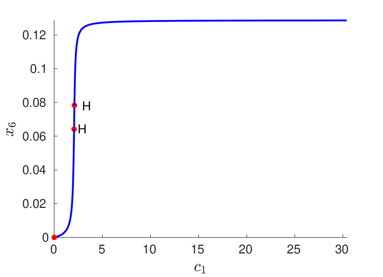
(a) $x_{6}$ vs. $c_{1}$

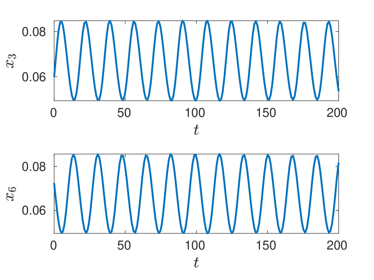
(b) $x_{3}$ and $x_{6}$ vs. $t$

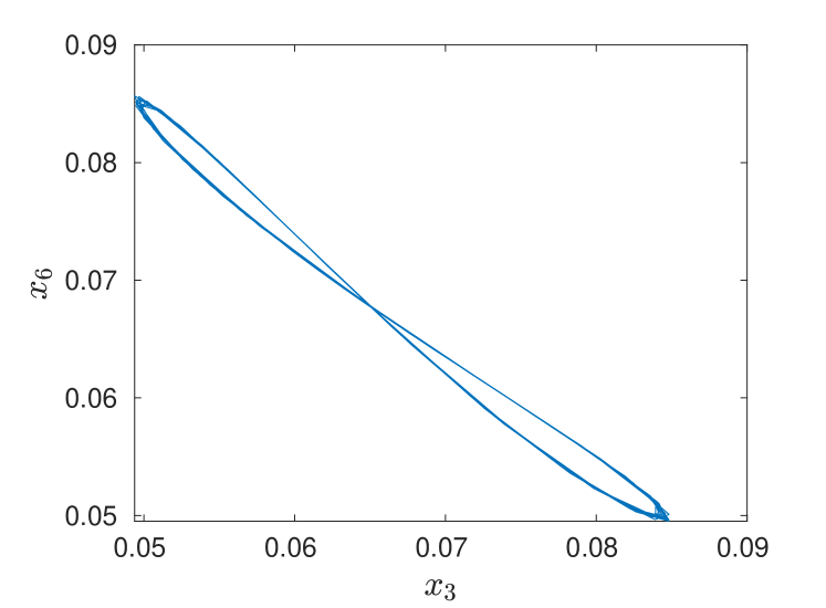
(c) $x_{6}$ vs. $x_{3}$

Figure 2: Numerical verification of Hopf bifurcations (panel (2(a)), labeled $H$) and a limit cycle (panel (2(b)) and (2(c))). Rate constants $k$ as in Table 2 with $\lambda=1$. Initial value $x(0)$ as in (LABEL:eq:h_x0_exa) – apart from $x_{3}(0)$ and $x_{6}(0)$: to obtain an initial value near the steady state $x$ given in (LABEL:eq:h_x0_exa) we choose $x_{3}(0)=1.1\cdot\frac{1}{15}$ and $x_{6}(0)=0.9\cdot\frac{1}{15}$).

Remark 3.8.

In the course of Steps 1 – 6 above all rate constants are fixed:

1. From (14) one obtains for network (3) the relation (29) between the $\kappa_{i}$ and the $h_{i}$.

2. Thus, choosing numerical values for $h_{7}$, …, $h_{10}$ is equivalent to choosing $\kappa_{3}$, $\kappa_{6}$, $\kappa_{9}$ and $\kappa_{12}$ (up to the factor $\lambda$).

3. Choosing numerical values for $h_{4}$ and $h_{5}$ and assigning $h_{1}=h_{2}=h_{3}=h_{6}=t$ is equivalent to choosing $\kappa_{1}$, $\kappa_{4}$, $\kappa_{7}$ and $\kappa_{10}$ (again up to the factor $\lambda$). In this case $\kappa_{1}$ and $\kappa_{7}$ are proportional to $t^{2}$ and $\kappa_{4}$ and $\kappa_{10}$ to $t$ – as $h_{4}$ and $h_{5}$ are fixed to numerical values.

4. For $h_{7}$, …, $h_{10}$ chosen in Step 1 and $\lambda=1$ one thus obtains $k=\left(t^{2},1,t,1,t^{2},1,t,2\right)$.

3.4 Lifting to the full network (1)

In [2] network modifications are described that preserve the existence of a stable positive limit cycle. This is the basis for the following result:

Theorem 3.9.

Consider networks (1) and (3). Assume the rate constant values of network (3) are such that the system (25a) – (25j) admits a stable limit cycle. Choose these values for the rate constants of network (1). For values of $\kappa_{2}$, $\kappa_{5}$, $\kappa_{8}$, $\kappa_{11}$ small enough, there exists a stable limit cycle in the system (24a) – (24j) close to the limit cycle of the system (25a) – (25j).

Proof.

In the language of [2], if, a network that admits a stable positive limit cycle (for some values of the rate constants and initial conditions) is modified by adding reactions that are in the span of the stoichiometric matrix, then the new network also admits a stable positive limit cycle [2, Theorem 1] (if the rate constants of the new reactions are chosen appropriately).

As the reaction vectors of reversible reactions are in the span of the stoichiometric matrix, the existence of a limit cycle in network (3) implies the existence of a limit cycle in the full network (1) for appropriately chosen rate constants of the backward reactions. ∎

To illustrate Theorem 3.9, we use the ODEs (24a) – (24j) and the values of Table 2 (on page 2). Fig. 3 demonstrates the existence of a limit cycle in the full system (24a) – (24j)(for $k_{b}$ sufficiently small).

Remark 3.10 (Locating the limit cycle in Fig. 3(a)).

For simplicity we choose $\kappa_{2}=\kappa_{5}=\kappa_{8}=\kappa_{11}=k_{b}$. To obtain Fig. 3 the initial value given in the table of Fig. 3(c) was used. This point is ‘close’ to the limit cycle of the ODEs defined by network (3) (i.e. for $k_{b}=0$). It was obtained by solving the ODEs (24a) – (24j) using Matlab’s ode15s with initial value given in Table 2 (on page 2) for a ‘long’ time (i.e. until $T=5000$) and $\lambda=1$. The point in the table of Fig. 3(c) corresponds to the last point of that first simulation.

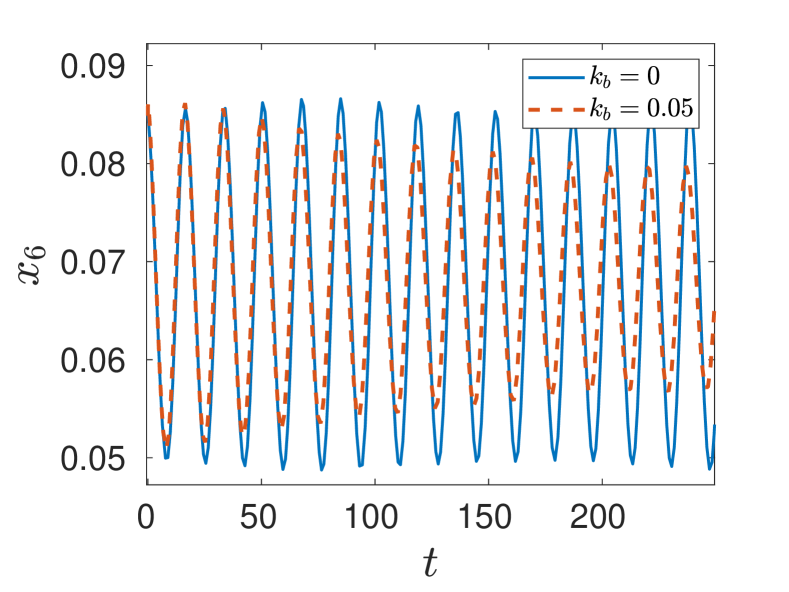
(a) $x_{6}$ vs. $t$ for $k_{b}=0$, $0.05$.

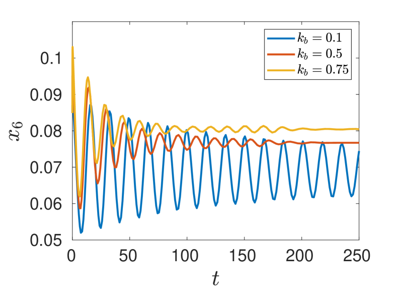
(b) $x_{6}$ vs. $t$ for $k_{b}=0.1$, $0.5$, $0.75$.

$x_{1}$	$x_{2}$	$x_{3}$	$x_{4}$	$x_{5}$	$x_{6}$	$x_{7}$	$x_{8}$	$x_{9}$	$x_{10}$
0.0885267	0.0528367	0.0496013	0.74587	1.261	0.084892	0.97124	1.0069	0.49383	1.02

(c) Initial value for simulations displayed in Fig. 3.

Figure 3: Simulation of network (1) for $\kappa_{2}=\kappa_{5}=\kappa_{8}=\kappa_{11}=k_{b}$ and different values $k_{b}$ (ODEs have been solved with ode15s (Mathworks) for $x(0)$ as in the table of panel (3(c)) and $\kappa_{i}$, $c_{i}$ as in Table 2 (on page 2 with $\lambda=1$). Panel (3(a)): $k_{b}=0$ corresponds to the ODEs derived from network (3), $k_{b}=0.05$ to the ODES (24a) – (24j) for $k_{b}=0.05$. The oscillations indicate for $k_{b}=0.05$ a stable limit cycle close to the stable limit cycle for $k_{b}=0$. Panel (3(b)): the stable limit cycle does not seem to exist for larger values of $k_{b}$.

4 Discussion

In this section we discuss inequality (2) in the light of results on multistationarity for a network of sequential distributive double phosphorylation described in [9]. In Section 4.1 we introduce the corresponding reaction network and compare it to network (1). In Section 4.2 we briefly summarize the results presented in Section 3 and in Section 4.3 the multistationarity results of [9]. We close by arguing our conclusion that in distributive double phosphorylation the catalytic constants enable non-trivial dynamics in Section 4.4.

4.1 Cyclic versus sequential distributive double phosphorylation

Sequential and distributive double phosphorylation can be described by the following mass action network (cf. e.g. [16] or [9]):

$$\begin{split}S_{0}+K\ce{<=>[\kappa_{1}][\kappa_{2}]}KS_{0}\ce{->[\kappa_{3}]}S_{1}+K\ce{<=>[\kappa_{4}][\kappa_{4}]}KS_{1}\ce{->[\kappa_{6}]}S_{2}+K\\ S_{2}+F\ce{<=>[\kappa_{7}][\kappa_{8}]}FS_{2}\ce{->[\kappa_{9}]}S_{1}+F\ce{<=>[\kappa_{10}][\kappa_{11}]}FS_{1}\ce{->[\kappa_{12}]}S_{0}+F.\end{split}$$ (38)

Network (38) is structurally similar to network (1): both networks contain 12 reactions and the only difference is that network (1) contains two species of mono-phosphorylated protein ($S_{10}$ and $S_{01}$), while network(38) contains only one ($S_{1}$). Hence network (38) contains nine species, while network network (1) contains ten.

In particular, networks (1) and (38) contain the same four phosphorylation events: (i) the conversion of unphosphorylated protein to mono-phosphorylated protein catalyzed be the kinase $K$, (ii) the conversion of mono-phosphorylated protein to double-phosphorylated protein catalyzed by the same kinase $K$, (iii) the conversion of double-phosphorylated protein to mono-phosphorylated protein catalyzed by the phosphatase $F$ and (iv) the conversion of mono-phosphorylated protein to unphosphorylated protein catalyzed by the same phosphatase $F$. As described in [9], in enzyme kinetics research it is customary to characterize such phosphorylation events by three constants, the Michaelis constant ($K_{m}$), the catalytic constant ($k_{c}$) and the equilibrium constant $k_{eq}$ of the respective enzyme substrate pair (see, for example, [3] for details on enzyme kinetics).

Of particular interest in the context of the present publication are the $k_{c}$-values as these correspond to the rate constants involved in inequality (2): $\kappa_{3}$ is the $k_{c}$-value of the kinase $K$ with unphosphorylated substrate ($S_{00}$ or $S_{0}$), $\kappa_{6}$ of $K$ with mono-phosphorylated substrate ($S_{10}$ or $S_{1}$), $\kappa_{9}$ of $F$ with double-phosphorylated substrate ($S_{11}$ or $S_{2}$) and $\kappa_{12}$ of $F$ with mono-phosphorylated substrate ($S_{10}$ or $S_{1}$).

4.2 Cyclic and distributive: emergence of oscillations

By Theorem 3.4, if these catalytic constants satisfy inequality (2), then there exists positive steady states of network (3) such that the Jacobian has a complex-conjugate pair of eigenvalues on the imaginary axis. This is necessary for a simple Hopf-bifurcation. If there is a supercritical simple Hopf bifurcation and a stable limit cycle emerges, then by Theorem 3.9 there is a stable limit cycle in network (1). Hence we say that for cyclic and distributive double phosphorylation the catalytic constants enable the emergence of oscillations.

4.3 Sequential and distributive: emergence of bistability

In [9] we have shown that the inequality (2) is sufficient for multistationarity in network (38). To be more precise, by [9, Theorem 5.1], if the catalytic constants satisfy inequality (2), then there exists values of the total concentrations of kinase, phosphatase and protein such that network (38) has three positive steady states – no matter what values the other rate constants take. As multistationarity is necessary for bistability, we say in [9], that the catalytic constants enable the emergence of bistability in sequential and distributive double phosphorylation.

4.4 Catalytic constants and non-trivial dynamics

In the previous subsections we have described how the catalytic constants of cyclic distributive double phosphorylation enable the emergence of oscillations, and how the catalytic constants of sequential distributive double phosphorylation enable the emergence of bistability. Hence we conclude that in distributive double phosphorylation the catalytic constants enable non-trivial dynamics.

As a consequence, if the rate constant are chosen according to the procedure of Section 3.3 and Theorem 3.9 and network (1) admits a stable limit cycle for these rate constants, then network (38) taken with the same rate constant values will show multistationarity – for some, usually different, value of the total concentrations. That is, if the catalytic constants satisfy (2), then a cyclic mechanism can show sustained oscillations, while a sequential mechanism equipped with the same rate constant values can show bistability.

As an example the procedure described in Section 3.3 together with Theorem 3.9 have been used to obtain the following rate constant values:

$$\kappa_{1} =49 \kappa_{2} =\frac{1}{10} \kappa_{3} =\frac{1}{2} \kappa_{4} =7$$

$$\kappa_{5} =\frac{1}{10} \kappa_{6} =2 \kappa_{7} =49 \kappa_{8} =\frac{1}{10}$$ (39)

$$\kappa_{9} =\frac{1}{4} \kappa_{10} =7 \kappa_{11} =\frac{1}{10} \kappa_{12} =\frac{3}{4}$$

These values satisfy inequality (2). Using these values in the ODEs derived from network (1), one detects simple Hopf bifurcations and oscillations as depicted in Fig. 4(a) and Fig. 4(b). And using these values in the ODEs derived from network (38), one obtains multistationarity as depicted in Fig. 4(c). To create these figures, the same parameter values have been used in both ODE systems, albeit for different values of the total concentrations. For Fig. 4(a) and Fig. 4(b) the procedure of Section 3.3 yields

$$c_{1}=\frac{37}{14},\;c_{2}=\frac{115}{21}\text{ and }c_{3}=\frac{425}{42},$$ (40)

where $c_{1}$ denotes total amount of kinase $K$, $c_{2}$ of phosphatase $F$ and $c_{3}$ of substrate $S$. And for Fig. 4(c) following the results of [9] yields (using the same notation for the total concentrations)

$$c_{1}=\frac{307}{27},\;c_{2}=\frac{650}{27}\text{ and }c_{3}=\frac{18539}{540}\ .$$ (41)

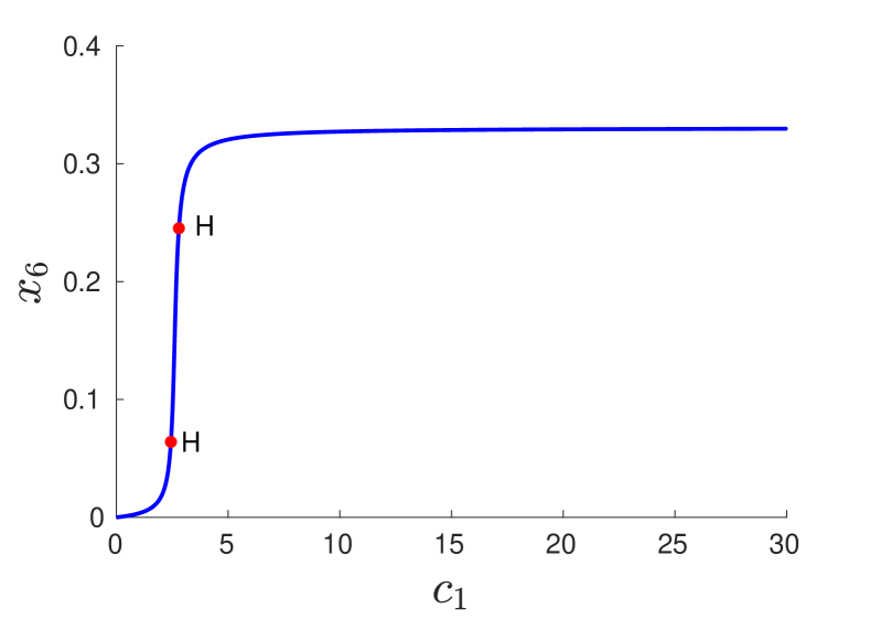
(a) Cyclic: numerical continuation of steady states. Steady state value of $S_{11}$ ($x_{6}$) vs. total concentration of Kinase $K$ ($c_{1}$); Hopf points (H).

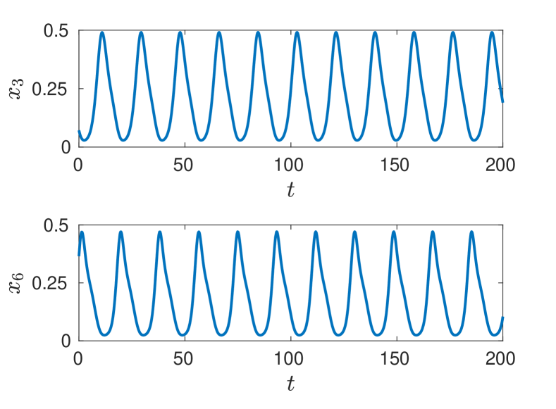
(b) Cyclic: numerical solutions of ODEs defined by network (1); plotting $S_{00}$ ($x_{3}$) and $S_{11}$ ($x_{6}$) vs. time $t$ shows sustained oscillations.

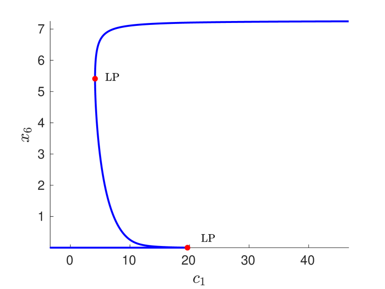
(c) Sequential: numerical continuation of steady states; $S_{2}$ ($x_{6}$) vs. $c_{1}$; LP limit point, multistationarity for $c_{1}$ between LPs.

Figure 4: Oscillations and multistationarity in distributive phosphorylation. Panel (a) & (b) Hopf bifurcations (H) and sustained oscillations in network (1); panel (c) multistationarity in network (38). Rate constants for both networks as in (39), total concentrations for network (1) in eq. (40) and for network (38) in eq. (41).

5 Data availability

Data sharing not applicable to this article as no datasets were generated or analyzed during the current study.

Appendix A A Remark on matrices of the form $A=\lambda B$

Throughout this section let $A,B\in\mathbb{R}^{n\times n}$ and $\lambda$ be a nonzero real number such that

$$A=\lambda B$$

Lemma A.1.

For matrices $A$, $B$ as above one has

$$\det(A)=\lambda^{n}\det(B)\ .$$

Proof.

If $B$ is singular, then $A$ is singular by construction and the result follows immediately. Otherwise the result follows by Laplace expansion of $\lambda B$. ∎

As in, for example, [17], for $A\in\mathbb{R}^{n\times n}$ let $E_{k}(A)$ denote the sum of the principal minors of size $k$ of the matrix $A$.

Lemma A.2.

For matrices $A$, $B$ as above one has

$$E_{k}(A)=\lambda^{k}E_{k}(B)\ .$$

Proof.

This follows from Lemma A.1 and the fact that $E_{k}(A)$ is a sum of determinants of $k\times k$-sub-matrices. ∎

Let $a_{k}$ denote the coefficients of the characteristic polynomial of $A$ and $b_{k}$ those of the characteristic polynomial of $B$.

Lemma A.3.

For $A$, $B$ as above

$$a_{k}=\lambda^{k}b_{k}\ .$$

Proof.

This follows from Lemma A.2 and and the fact that the coefficients $a_{k}$ of any $n\times n$ matrix can be defined in terms of the sums of $k\times k$ principal minors of $A$ (cf. [17, eq. (1.2.13)]):

$$a_{k}=(-1)^{n-k}E_{k}(A)\ .$$

∎

And finally:

Lemma A.4.

Let $A$, $B$ be as above and assume that $\operatorname{rank}(A)=\operatorname{rank}(B)=s<n$. Then the characteristic polynomial of $A$ can be expressed in terms of the characteristic polynomial of $B$ by the following formula:

$$\det(\mu I_{n}-\lambda A) =\mu^{n-s}\left(\mu^{s}+\lambda b_{1}\mu^{s-1}+\ldots+\lambda^{s-1}b_{s-1}\mu+\lambda^{s}b_{s}\right)$$ (42)

$$=\mu^{n-s}\lambda^{s}\left(\left(\frac{\mu}{\lambda}\right)^{s}+\sum_{i=1}^{s}\lambda^{i}b_{i}(h)\left(\frac{\mu}{\lambda}\right)^{s-i}\right)$$ (43)

Proof.

Eq. (42) follows from Lemma A.2 and [17, eq. (1.2.13)], eq. (43) by factoring $\lambda^{s}$ (which is well defined as in our setting $\lambda\neq 0$). ∎

Appendix B Hurwitz determinants of $H(\lambda,h)$ and $G(h)$

Recall that $s=\operatorname{rank}(S)$, where $S$ is the $n\times m$ stoichiometric matrix. By Corollary 2.2 we have $a_{i}=\lambda^{i}b_{i}(h)$, $i=1,2,\ldots,s$.

We use the following formula for the determinant of a matrix $A$ with elements $a_{ij}$, $i$, $j=1$, …$n$ proved in [20]

$$\det A=\sum_{\sigma}(-1)^{n+f}A[c_{1}]\ldots A[c_{f}],$$ (44)

where $c_{1},\ldots,c_{f}$ are pairwise disjoint cycles of a permutation $\sigma$. For a cycle $c=(i_{1},i_{2},\ldots,i_{k})$ we have,

$$A[c]=a_{i_{2}i_{1}}a_{i_{3}i_{1}}\ldots a_{i_{1},i_{k}}\ .$$

We define the differences between two consecutive indices in a cycle $c=(i_{1},\ldots,i_{k})$:

Definition 3.

Let $c=(i_{1},i_{2},\ldots,i_{k})$ be a cycle. We define the (cycle) differences $d_{i_{s}i_{s+1}}=i_{s}-i_{s+1}$, $s=1,\ldots,k$, where $i_{k+1}=i_{1}$ between any two consecutive indices of $c$.

The lemma below follows immediately by (44) and the differences’ definition. In (46) we state a different formulation of the product $H_{l}[c]$, with the help of the differences of a cycle $c$, which is specific to Hurwitz matrices. The same lemma applies to the Hurwitz matrices $G_{l}(h)$, $l=1,2,\ldots,s$.

Lemma B.1.

Let $\det H_{l}$ be the Hurwitz determinant of $l$-th order, $l=1,2,\ldots,s$. Then

$$\det H_{l}=\sum_{\sigma}(-1)^{l+f}H_{l}[c_{1}]\ldots H_{l}[c_{f}]$$ (45)

where $\sigma$ is a permutation and $c_{1},\ldots,c_{f}$ are the set of corresponding pairwise disjoint cycles of $\sigma$. We have for a cycle $c=(i_{1},\ldots,i_{k})$ and the corresponding product

$$H_{l}[c]=a_{2i_{1}-i_{2}}a_{2i_{2}-i_{3}}\ldots a_{2i_{k}-i_{1}}=a_{i_{1}+d_{i_{1}i_{2}}}a_{i_{2}+d_{i_{2}i_{3}}}\ldots a_{i_{k}+d_{i_{k}i_{1}}}\ .$$ (46)

The next lemma follows immediately by Definition 3.

Lemma B.2.

Let $c=(i_{1},i_{2},\ldots,i_{k})$ be a cycle. For any cycle $c$, the sum of its differences is zero, $d_{i_{1}i_{2}}+d_{i_{2}i_{3}}+\ldots+d_{i_{k}i_{1}}=0\,.$

Remark B.3.

We notice that $\det H_{l}(1,h)=\det G_{l}(h)$ for $l=1,2,\ldots s$ if $\lambda=1$.

Now we can turn to the proof of Proposition 2.4:

Proof of Proposition 2.4.

Let $c=(i_{1},\ldots,i_{k})$ be a cycle. By by Corollary 2.2 we have for the product $a_{i_{1}}\ldots a_{i_{k}}$

$$a_{i_{1}}\ldots a_{i_{k}}=\lambda^{\delta}b_{i_{1}}\ldots b_{i_{k}},\text{ where $\delta=i_{1}+\ldots+i_{k}$.}$$

By Lemma B.1 and in particular (46)

$$\begin{split}H_{l}[c]&=a_{i_{1}+d_{i_{1}i_{2}}}\ldots a_{i_{k}+d_{i_{k}i_{1}}}=\lambda^{i_{1}+d_{i_{1}i_{2}}}b_{i_{1}+d_{i_{1}i_{2}}}\ldots\lambda^{i_{k}+d_{i_{k}i_{1}}}b_{i_{k}+d_{i_{k}i_{1}}}\\ &=\lambda^{\delta}b_{i_{1}}\ldots b_{i_{k}}=\lambda^{\delta}G_{l}[c]\end{split}$$ (47)

where we have used that the sum of the differences of a cycle sum up to zero by Lemma B.2.

Let the sum of the indices of each cycle $c_{1},,\ldots c_{f}$ of a permutation $\sigma$ be denoted by $\delta_{1}$, …,$\delta_{f}$, correspondingly. We use the fact that the cycles $\{c_{1},\ldots,c_{f}\}$ in a permutation $\sigma$ are pairwise disjoint. Thus it follows that

$$\delta_{1}+\delta_{2}+\ldots+\delta_{f}=1+2+\ldots+l=\frac{l(l+1)}{2}.$$ (48)

By Lemma B.1, (47) and (48) we have

$$\det H_{l}(\lambda,h)= \Sigma_{\sigma}(-1)^{l+f}H_{l}[c_{1}]\ldots H_{l}[c_{f}]$$

$$=\Sigma_{\sigma}(-1)^{l+f}\lambda^{\delta_{1}}G_{l}[c_{1}]\ldots\lambda^{\delta_{f}}G_{l}[c_{f}]$$

$$=\Sigma_{\sigma}(-1)^{l+f}\lambda^{\delta_{1}+\ldots+\delta_{f}}G_{l}[c_{1}]\ldots G_{l}[c_{f}]$$

$$=\lambda^{l(l+1)/2}\Sigma_{\sigma}(-1)^{l+f}G_{l}[c_{1}]\ldots G_{l}[c_{f}]$$

$$=\lambda^{l(l+1)/2}\det G_{l}(h)\ .$$

Thus, $\det H_{l}(\lambda,h)=\lambda^{l(l+1)/2}\det G_{l}(h)$ for $l=1,2,\ldots,s$. ∎

Appendix C Data for network (3)

$S_{00}+K$	$y^{(1)}=(1,0,1,0,0,0,0,0,0,0)^{T}$
$S_{00}K$	$y^{(2)}=(0,0,0,0,0,0,1,0,0,0)^{T}$
$S_{10}+K$	$y^{(3)}=(1,0,0,1,0,0,0,0,0,0)^{T}$
$S_{10}K$	$y^{4)}=(0,0,0,0,0,0,0,1,0,0)^{T}$
$S_{11}+K$	$y^{(5)}=(1,0,0,0,0,1,0,0,0,0)^{T}$
$S_{11}+F$	$y^{(6)}=(0,1,0,0,0,1,0,0,0,0)^{T}$
$S_{11}F$	$y^{(7)}=(0,0,0,0,0,0,0,0,0,1)^{T}$
$S_{01}+F$	$y^{(8)}=(0,1,0,0,1,0,0,0,0,0)^{T}$
$S_{01}F$	$y^{(9)}=(0,0,0,0,0,0,0,0,1,0)^{T}$
$S_{00}+F$	$y^{(10)}=(0,1,1,0,0,0,0,0,0,0)^{T}$

Table 3: Complexes of network (1) and (3).

The stoichiometric matrix $S$, the exponent matrix $Y$ and a matrix $W$ defining the conservation relations:

$$\begin{split}\tiny S&=\left[\begin{array}[]{rrrrrrrr}-1&1&-1&1&0&0&0&0\\ 0&0&0&0&-1&1&-1&1\\ -1&0&0&0&0&0&0&1\\ 0&1&-1&0&0&0&0&0\\ 0&0&0&0&0&1&-1&0\\ 0&0&0&1&-1&0&0&0\\ 1&-1&0&0&0&0&0&0\\ 0&0&1&-1&0&0&0&0\\ 0&0&0&0&0&0&1&-1\\ 0&0&0&0&1&-1&0&0\\ \end{array}\right],\;Y=\left[\begin{array}[]{rrrrrrrr}1&0&1&0&0&0&0&0\\ 0&0&0&0&1&0&1&0\\ 1&0&0&0&0&0&0&0\\ 0&0&1&0&0&0&0&0\\ 0&0&0&0&0&0&1&0\\ 0&0&0&0&1&0&0&0\\ 0&1&0&0&0&0&0&0\\ 0&0&0&1&0&0&0&0\\ 0&0&0&0&0&0&0&1\\ 0&0&0&0&0&1&0&0\\ \end{array}\right],\\ W^{T}&=\begin{bmatrix}1&0&0&0&0&0&1&1&0&0\\ 0&1&0&0&0&0&0&0&1&1\\ 0&0&1&1&1&1&1&1&1&1\\ \end{bmatrix}\end{split}$$

The vector of rate functions is

$$v(k,x)=(\kappa_{1}x_{1}x_{3},\kappa_{3}x_{7},\kappa_{4}x_{1}x_{4},\kappa_{6}x_{8},\kappa_{7}x_{2}x_{6},\kappa_{9}x_{10},\kappa_{10}x_{2}x_{5},\kappa_{12}x_{9})^{T}\;.$$ (49)

The diagonal matrix of rate constants

$$\operatorname{diag}(k)=\left[\begin{array}[]{cccccccc}k_{1}&0&0&0&0&0&0&0\\ 0&k_{2}&0&0&0&0&0&0\\ 0&0&k_{3}&0&0&0&0&0\\ 0&0&0&k_{4}&0&0&0&0\\ 0&0&0&0&k_{5}&0&0&0\\ 0&0&0&0&0&k_{6}&0&0\\ 0&0&0&0&0&0&k_{7}&0\\ 0&0&0&0&0&0&0&k_{8}\\ \end{array}\right]$$

The vector of monomials of the rate function $v(k,x)$

$$\phi(k,x)=(x_{1}x_{3},x_{7},x_{1}x_{4},x_{8},x_{2}x_{6},x_{10},x_{2}x_{5},x_{9})^{T}\;.$$

Appendix D Initial data for Fig. 4(a) & 4(b)

To generate Fig. 4(a) & 4(b) the ODEs derived from the full (reversible) reaction network (1) are used (i.e. the ODEs (24a) – (24j)). In both Fig. 4(a) and 4(b) we use the point displayed in Table 4 as initial value.

$x_{1}$	$x_{2}$	$x_{3}$	$x_{4}$	$x_{5}$	$x_{6}$	$x_{7}$	$x_{8}$	$x_{9}$	$x_{10}$
$\frac{1}{7}$	$\frac{1}{7}$	$\frac{1}{7}$	$1$	$1$	$\frac{1}{7}$	$2$	$\frac{1}{2}$	$\frac{4}{3}$	$4$

Table 4: Initial value for Fig. 4(a) & 4(b)

Remark D.1.

The point in Table 4 is a steady state of the irreversible network (3) generated according to our procedure (with $h_{7}=\frac{1}{2}$, $h_{8}=2$, $h_{9}=\frac{3}{4}$, $h_{10}=\frac{1}{4}$, $h_{4}=h_{5}=1$ and $t=1$).

We use Matlab’s ode15s to solve the initial value problem defined by the above ODEs with initial value given in Table 4 and the backward constants $\kappa_{2}=\kappa_{5}=\kappa_{8}=\kappa_{11}=\frac{1}{10}$ (and the remaining constants according to our procedure for the irreversible network). These backward constants are ‘small enough’ in the sense of the results of [2], that is, that the reversible network (1) has a limit cycle close to the limit cycle of the irreversible network.

However, on the one hand the steady state of Table 4 (of the irreversible network) is ‘far enough’ from a steady state of the reversible network in the following sense: the solution of the reversible system with initial value given in Table 4 approaches a limit cycle of the reversible system (if approximated with ode15s). If the point given in Table 4 was ‘too close’ to a steady state of the reversible system the solution with it as initial value would approach that steady state (if approximated with ode15s).

On the other hand, Fig. 4(a) is generated with Matcont using the point given in Table 4 as an initial guess of a steady state of the above ODEs (of the reversible network). And this point is close enough to a steady state of the reversible network for Matcont to converge to a steady state.

Appendix E Initial data for Fig. 4(c)

To obtain Fig. 4(c) we follow [9], where a system of nine ODEs is derived from network (38). As in this reference, we use the variables given in Table 5 to denote the species concentrations. As this network does not distinguish $S_{10}$ and $S_{01}$, there is only one mono-phosphorylated from of the substrate ($S_{1}$) and $S_{2}$ is used to denote the double-phosphorylated substrate. Consequently, this network contains only nine species. It has, however, $12$ reactions and the labeling is consistent with network (1).

$x_{1}$	$x_{2}$	$x_{3}$	$x_{4}$	$x_{5}$	$x_{6}$	$x_{7}$	$x_{8}$	$x_{9}$
$S_{0}$	$K$	$KS_{0}$	$S_{1}$	$KS_{1}$	$S_{2}$	$F$	$FS_{2}$	$FS_{1}$

Table 5: Variables and species for network (38) (as in [9]).

Using the approach described in [9] we obtain the steady state depicted in Table 6. We use this point as a starting point for the numerical continuation in Matcont.

$x_{1}$	$x_{2}$	$x_{3}$	$x_{4}$	$x_{5}$	$x_{6}$	$x_{7}$	$x_{8}$	$x_{9}$
$\frac{1}{10}$	$1$	$\frac{49}{6}$	$\frac{119}{180}$	$\frac{119}{54}$	$\frac{17}{135}$	$1$	$\frac{476}{27}$	$\frac{49}{9}$

Table 6: Starting point for the numerical continuation in Fig. 4(c) (a steady state of network (38) for the rate constant values of eq. (39) generated as described in [9]).

Acknowledgments

Maya Mincheva wishes to thank the Institute of Mathematics and Informatics at the Bulgarian Academy of Sciences where part of this research was done for their hospitality.

Carsten Conradi was partially funded by DFG Grant 517274113.

MM and CC thank all reviewers for their diligent review and helpful suggestions.

References

- [1] Benjamin Assarf, Ewgenij Gawrilow, Katrin Herr, Michael Joswig, Benjamin Lorenz, Andreas Paffenholz, and Thomas Rehn, Computing convex hulls and counting integer points with polymake, Mathematical Programming Computation 9 (2017), no. 1, 1–38.
- [2] Murad Banaji, Inheritance of oscillation in chemical reaction networks, Applied Mathematics and Computation 325 (2018), 191 – 209.
- [3] Athel Cornish Bowden, Fundamentals of enzyme kinetics, Portland Press, London, 2004.
- [4] Thomas Höfer Carlos Salazar, Versatile regulation of multisite protein phosphorylation by the order of phosphate processing and protein-protein interactions, FEBS Journal 274 (2007), 1046–1061.
- [5] Bruce L. Clarke, Stoichiometric network analysis, Cell Biophysics 12 (1988), 237–253.
- [6] Carsten Conradi, Elisenda Feliu, and Maya Mincheva, On the existence of Hopf bifurcations in the sequential and distributive double phosphorylation cycle, Mathematical Biosciences and Engineering 17 (2020), no. mbe-17-01-027, 494.
- [7] Carsten Conradi and Dietrich Flockerzi, Multistationarity in mass action networks with applications to ERK activation, Journal of Mathematical Biology 65 (2012), no. 1, 107–156.
- [8] Carsten Conradi, Dietrich Flockerzi, and Jörg Raisch, Multistationarity in the activation of an MAPK: parametrizing the relevant region in parameter space, Mathematical Biosciences 211 (2008), no. 1, 105–131.
- [9] Carsten Conradi and Maya Mincheva, Catalytic constants enable the emergence of bistability in dual phosphorylation, Journal of The Royal Society Interface 11 (2014), no. 95.
- [10] Carsten Conradi, Maya Mincheva, and Anne Shiu, Emergence of oscillations in a mixed-mechanism phosphorylation system, Bulletin of Mathematical Biology 81 (2019), no. 6, 1829–1852.
- [11] Carsten Conradi and Casian Pantea, Chapter 9 - multistationarity in biochemical networks: Results, analysis, and examples, Algebraic and Combinatorial Computational Biology (Raina Robeva and Matthew Macauley, eds.), Academic Press, 2019, pp. 279 – 317.
- [12] Carsten Conradi and Anne Shiu, A global convergence result for processive multisite phosphorylation systems, Bulletin of Mathematical Biology 77 (2015), no. 1, 126–155.
- [13] Carsten Conradi and Anne Shiu, Dynamics of posttranslational modification systems: Recent progress and future directions, Biophysical Journal 114 (2018), no. 3, 507 – 515.
- [14] Ewgenij Gawrilow and Michael Joswig, polymake: a Framework for Analyzing Convex Polytopes, Polytopes – Combinatorics and Computation, Birkhäuser Basel, Basel, 2000, pp. 43–73.
- [15] Juliette Hell and Alan D. Rendall, A proof of bistability for the dual futile cycle, Nonlinear Analysis: Real World Applications 24 (2015), 175–189.
- [16] Katharina Holstein, Dietrich Flockerzi, and Carsten Conradi, Multistationarity in sequential distributed multisite phosphorylation networks, Bulletin of Mathematical Biology 75 (2013), no. 11, 2028–2058.
- [17] Roger A. Horn and Charles R. Johnson, Matrix analysis, 2 ed., Cambridge University Press, 2012.
- [18] Yu A Kuznetsov, Matcont: a matlab package for numerical bifurcation analysis of odes, ACM Transactions on Mathematical Software (TOMS) 29 (2003), no. 2, 141–164.
- [19] W. M. Liu, Criterion of Hopf Bifurcations without Using Eigenvalues, Journal of Mathematical Analysis and Applications 182 (1994), no. 1, 250 – 256.
- [20] John S Maybee, DD Olesky, Driessche P van den, and G Wiener, Matrices, digraphs, and determinants, SIAM Journal on Matrix Analysis and Applications 10 (1989), no. 4, 500–519.
- [21] Vaidhiswaran Ramesh, Thapanar Suwanmajo, and J. Krishnan, Network regulation meets substrate modification chemistry, Journal of The Royal Society Interface 20 (2023), no. 199, 20220510.
- [22] Ralph Tyrell Rockafellar, Convex analysis, Princeton University Press, 1970.
- [23] Carlos Salazar and Thomas Höfer, Multisite protein phosphorylation - from molecular mechanisms to kinetic models, FEBS Journal 276 (2009), no. 12, 3177–3198.
- [24] Thapanar Suwanmajo and J. Krishnan, Mixed mechanisms of multi-site phosphorylation, Journal of The Royal Society Interface 12 (2015), no. 107, 20141405.
- [25] , Exploring the intrinsic behaviour of multisite phosphorylation systems as part of signalling pathways, Journal of The Royal Society Interface 15 (2018), no. 143, 20180109.
- [26] Thapanar Suwanmajo, Vaidhiswaran Ramesh, and J. Krishnan, Exploring cyclic networks of multisite modification reveals origins of information processing characteristics, Scientific Reports 10 (2020), no. 1, 16542.
- [27] Máté László Telek and Elisenda Feliu, Topological descriptors of the parameter region of multistationarity: Deciding upon connectivity, PLOS Computational Biology 19 (2023), no. 3, 1–38.
- [28] Xiaojing Yang, Generalized form of Hurwitz-Routh criterion and Hopf bifurcation of higher order, Applied Mathematics Letters 15 (2002), no. 5, 615 – 621.