Performance Studies of the Acoustic Module for the IceCube Upgrade
Abstract
The IceCube Upgrade will augment the existing IceCube Neutrino Observatory by deploying 700 additional optical sensor modules and calibration devices within its center at a depth of 1.5 to 2.5 km in the Antarctic ice. One goal of the Upgrade is to improve the positioning calibration of the optical sensors to increase the angular resolution for neutrino directional reconstruction. An acoustic calibration system will be deployed to explore the capability of achieving this using trilateration of propagation times of acoustic signals. Ten Acoustic Modules (AM) capable of sending and receiving acoustic signals with frequencies from 5 to 30 kHz will be installed within the detector volume. Additionally, compact acoustic sensors inside 15 optical sensor modules will complement the acoustic calibration system. With this system, we aim for an accuracy of a few tens of cm to localize the Acoustic Modules and sensors. Due to the longer attenuation length of sound compared to light within the ice, acoustic position calibration is especially interesting for the upcoming IceCube-Gen2 detector, which will have a string spacing of around 240 m. In this contribution we present an overview of the technical design of the Acoustic Module as well as results of performance tests with a first complete prototype.
Corresponding authors:
Charlotte Benning1, Jürgen Borowka1, Christoph Günther1∗, Oliver Gries1, Simon Zierke1
1 RWTH Aachen University
∗ Presenter
1 Introduction
The IceCube Upgrade will improve the existing IceCube neutrino telescope by deploying approximately 700 new modules including photo sensors and multiple calibration devices at the bottom center of the detector. [1] These will be mounted on 7 new cable strings with a horizontal spacing of approximately 30 m and about 2 m vertically between modules along the strings.
The acoustic module (AM) is one of the new calibration devices. Ten AMs will be distributed over the Upgrade strings with distances ranging from a few tens of meters to 1000 m. The main goal is to explore the feasibility of geometrical calibration of the photo sensors by measuring the acoustic propagation times between the modules in the ice. An accuracy in the order of 1 ns cm is aimed as this will significantly improve the reconstruction of track-like signatures induced by high-energetic neutrinos [2].
A good knowledge of the acoustic ice properties, including the speed of sound and attenuation, is important. The South Pole Acoustic Test Setup (SPATS) has already performed measurements of the speed of sound [3] and attenuation length [4] down to a depth of m. The AM will enhance these results by measuring down to a depth of 2.5 km with improved accuracy.
The AMs operate as high-power sound emitters and receivers operating at frequencies in the nominal range of 5-30 kHz. The modules are integrated into the IceCube infrastructure and data-acquisition (DAQ). This allows timing accuracy of a few microseconds or better between the modules. The acoustic signals emitted by one module can be received by the others and propagation times are extracted from the acoustic waveforms using a dedicated analysis that extracts the group delay of chirp signals [5]. From the propagation times, the positions of the AMs are reconstructed using a likelihood fit. Acoustic sensors placed in some of the optical modules, namely the pDOMs [6], will allow the cross-calibration with optical methods and eventually a re-calibration of the existing IceCube detector. More details on these sensors can be found in [7].
Using acoustics for geometry calibration is promising as measurement results from SPATS indicate a long attenuation length in ice of up to a few hundred meters [4]. This is especially interesting for the IceCube Gen-2 detector with a planned string spacing of m [8]. Also, acoustics can be operated simultaneously to optical operation, allowing a large repetition rate to improve the signal-to-noise ratio (SNR) of the recorded waveforms.
In this paper, we present measurements with the first prototype of the AM which have been carried out in a local swimming pool. The emitting power and receiving sensitivity as function of frequency calculated from these measurements are used to estimate the nominal distance range for operation in the Antarctic ice.
2 Technical Design
The components of the AM are housed inside a powder-coated steel housing with a wall thickness of 1.5 cm, ensuring pressure resistance of up to 700 bar. A vacuum port allows to compensate for the atmospheric pressure difference between the production site and Antarctica to assure an under pressure inside the housing at all times. Cables for power supply and communication are fed into the module by a so-called Penetrator Cable Assembly (PCA), which is standardized for all IceCube Upgrade devices. All interfaces to the housing are sealed by multiple high-performance O-rings. Figure 1a shows an illustration of the AM and its internal components.
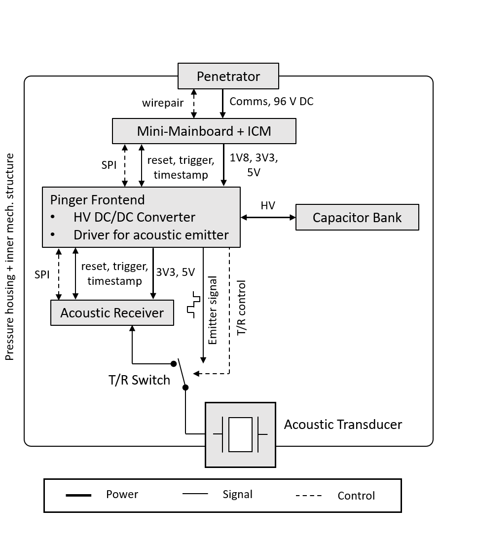
The electronic components consist of the Mini-Mainboard (MMB), Ice Comms Module (ICM), Pinger Front-end (PFE), capacitor bank, and receiver front-end. The MMB is used in multiple devices in the Upgrade and is responsible for command and data handling. It consists of two boards, the controller and the power board. The power board is the interface to the main in-ice cable and supplies all other components in the AM with power. The controller board has two main components: an STM32H7 microcontroller, which controls the front-end boards, and the ICM, which handles the communication to the surface, the timing as well as the power distribution.
The PFE generates the emitter signals to drive the acoustic transducer. It charges a ceramic capacitor bank (F) using a high voltage (HV) DC/DC converter with up to 320 V in about s. A full-bridge driver uses the energy stored in the capacitor bank to generate bipolar rectangular signals with frequencies from 5-30 kHz at a sampling rate of 1 MS/s. A sine wave is approximated by the 4 output states of the full-bridge driver (+HV, 0, -HV, 0). Therefore, possible signal frequencies are .
Relays on the PFE board allow switching between emitter and receiver mode. In receiver mode, only the receiver front-end is connected to the transducer and acoustic signals can be recorded with a sampling rate of up to kS/s. The gain of the receiver is dB @ 10 kHz and has a bandwidth of 5-30 kHz (@-3 dB). The gain can be adjusted by software to adapt to the level of the acoustic signals. Figure 1b shows a block diagram of the interconnections within the module.
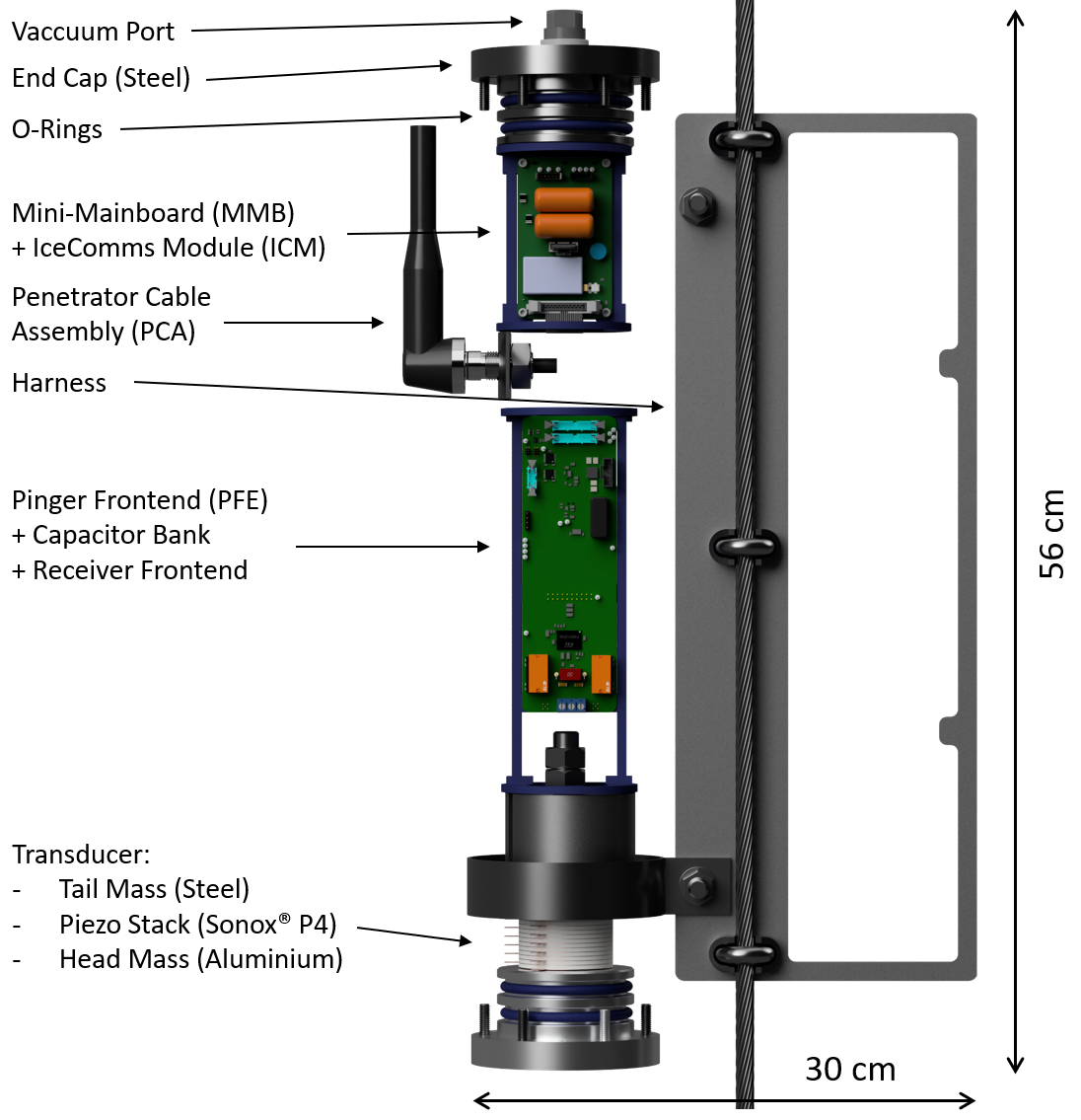
The acoustic transducer is a Tonpilz-style piezo transducer. It consists of a stack of 16 piezo discs clamped between an aluminum head-mass ( kg), which also acts as the enclosure cap of one side, and a steel tail-mass ( kg). The resulting mass ratio of increases the amount of sound emitted outwards of the module [9]. The transducer has a resonance frequency at kHz.
The AM will be attached to the Upgrade strings by a custom harness. It consists of two rings holding the AM which are connected to a mounting plate. Using three wire rope clamps the plate is attached to a 2 m steel rope with thimbles. Only the lowest clamp is fully tightened to prevent stress on the steel rope due to thermal expansion. Stoppers above and beyond the clamps prevent the module from slipping along the rope. A bracket allows to fixate the main cable. All of the harness components are made from stainless steel. More details on the technical design of the acoustic module can be found in [5].
3 Output Power
The acoustic output power is measured by the Transmitting Voltage Response (TVR), which is defined as the Sound Intensity Level (SIL) generated at a distance of 1 m by the transducer per 1 V of input voltage in dependence of frequency [10]:
| (1) |
The SIL can be measured by the output voltage of a transducer with known Open Circuit Receiving Response (OCRR). These are related by:
| (2) |
To measure the TVR, the AM is placed together with two absolutely calibrated ITC1001 hydrophones [11] in a large water volume (swimming pool). The output power of the AM is compared to that of an Autonomous Pinger Unit (APU), which has been developed within the EnEx-RANGE project for acoustic trilateration in glacial ice. The transducer design of the APU is very similar to that of the AM. Differences are the number of piezo discs (8 compared to 16) and the head-to-tail mass ratio (3:1 compared to 1:2.6) [12].
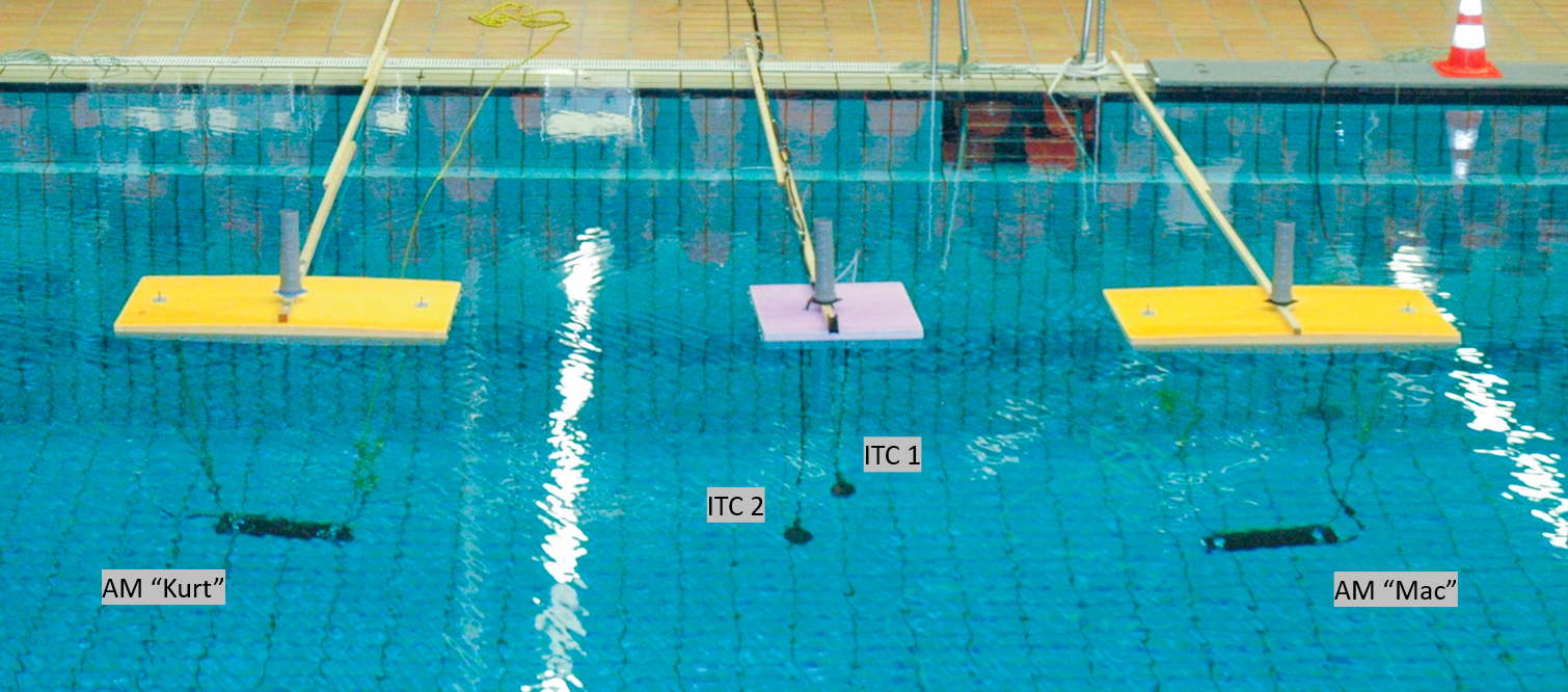
Figure 2 shows a picture of the measurement setup. The ITCs are placed in the center and separated by a distance of m from each module. The distance of the closest wall of the swimming pool is m. The exact locations of the probes have been measured to a precision of 10 cm using a laser odometer and reference tubes on top of the floating panels. For the emitter measurements, the right AM ("Mac") is emitting and the two ITCs are receiving the acoustic signals. The setup for the APU measurements is analogous.
During the emitter measurement, the AM and APU are charged to a voltage of V and emit sine bursts with a duration of 10 ms (5 ms for the APU). The frequency of the bursts is varied between 5 and 30 kHz. The ITCs are connected directly to an oscilloscope which triggers at a threshold of 100 mV on the rising edge of the output signal. Typical recorded amplitudes range from a few 100 mV to 2 V. Five waveforms are recorded for each frequency and are averaged in later analysis.
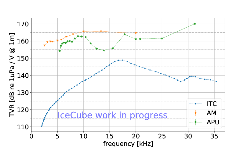
The SIL at the ITC is measured by the voltage root-mean-square (RMS) of the waveforms. Therefore, the baseline is subtracted and the RMS is computed in a window of 1 ms after the trigger threshold. The TVR of the AM and APU are calculated using equation 1. The TVR has been scaled to a distance of 1 m from pinger to ITC by assuming an attenuation of : .
The resulting TVR curves for the AM and the APU as well as for the ITC are shown in figure 3. The maximum output is reached for both of the modules at 10 kHz, which is the expected resonance frequency of the transducer. The output power of the AM is approximately 2-3 times higher compared to the APU. This can be explained by the increased number of piezo discs and the improved mass ratio of the transducer.
4 Range Estimation
The range of the AM is determined by the distance at which a minimum required SNR can be reached. During a measurement at the Langenferner glacier in Italy, the APU achieved an SNR of 100 at a distance of m from APU to APU by averaging 64 waveforms [12]. The attenuation length of the glacial ice was measured to be m [13]. In the Antarctic ice, however, measurements by SPATS at shallow depths (m) resulted in an attenuation length of approx. 300 m [4]. Knowing that the AMs are similar to the APU and that the ice is similar to SPATS, although a slightly smaller attenuation length is expected for the warmer ice at deeper depths, we expect an attenuation length somewhere in-between. Combining this information with the measurements described in the previous sections, an estimation of the AM’s range is drawn.
The acoustic signal amplitude and therefore the SNR is attenuated by a geometrical factor and an exponential attenuation: , whereas can be fitted with the measured data. Solving this for and requiring a minimal SNR of 10:1 this equation can be solved for the maximal achievable range :
| (3) |
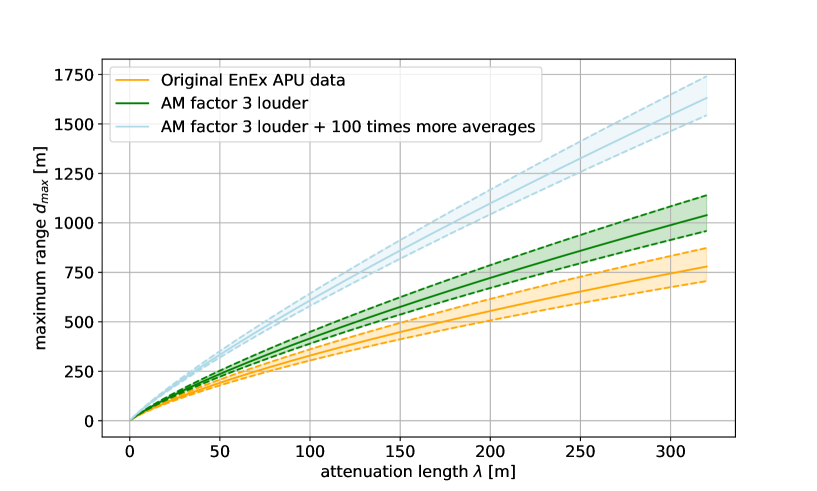
whereas is the Lambert W function and the minimum required signal amplitude. Figure 4 shows the resulting estimated range vs. attenuation length for the APU (orange) and also for assuming a factor of 3 more acoustic output power of the AM (green) as indicated by the measurement results. One can see that for an attenuation length of 300 m as indicated by measurements of SPATS a range of m is expected. By increasing the number of averages, the SNR can be increased proportionally to . For a more conservative estimate of 175 m for the attenuation length the same range is expected by averaging 100 times more waveforms. This is shown by the blue curve.
5 Conclusion
The in-water measurements indicate an improved output power of the AM by a factor of 2-3 compared to the APU. This indicates an estimated range of the AMs in the Antarctic ice of up to 1000 m or more. This is sufficient for the Upgrade configuration, which has a maximum distance between AMs of m. For the upcoming Gen-2 detector with a string spacing of 240 m this estimate makes acoustic calibration an interesting option for geometric calibration. Results from the Upgrade will give insight into important acoustic parameters of the Antarctic ice at unreached depths and will explore the feasibility for future acoustic in-ice calibration systems.
References
- [1] IceCube Collaboration, A. Ishihara PoS ICRC2019 (2019) 1031.
- [2] L. Peters Bachelor thesis, RWTH Aachen University, 2019. In German.
- [3] IceCube Collaboration, R. Abbasi et al. Astroparticle Physics 33 no. 5-6, (Jun, 2010) 277–286.
- [4] IceCube Collaboration, R. Abbasi et al. Astroparticle Physics 34 no. 6, (Jan, 2011) 382–393.
- [5] IceCube Collaboration, J. Borowka et al. PoS ICRC2021 (2021) 1059.
- [6] IceCube Collaboration, M. DuVernois PoS ICRC2015 (2016) 1148.
- [7] IceCube Collaboration, D. Heinen et al. PoS ICRC2019 (2019) 1030.
- [8] IceCube Gen-2 Collaboration, M. G. Aartsen et al. Journal of Physics G 48 no. 6, (Apr, 2021) 060501.
- [9] L. S. Weinstock. PhD thesis, RWTH Aachen University, 2019. in German.
- [10] J. Butler and C. Sherman, Transducers and Arrays for Underwater Sound. The Underwater Acoustics Series. Springer New York, NY, 2011.
- [11] Gavial, Model ITC-1001 - Spherical, Omnidirectional Transducer, 2017.
- [12] L. S. Weinstock et al. Annals of Glaciology (2020) 1–10.
- [13] A. Meyer, D. Eliseev, D. Heinen, P. Linder, F. Scholz, L. S. Weinstock, C. Wiebusch, and S. Zierke The Cryosphere 13 no. 4, (2019) 1381–1394.
Full Author List: IceCube-Gen2 Collaboration
R. Abbasi17,
M. Ackermann76,
J. Adams22,
S. K. Agarwalla47, 77,
J. A. Aguilar12,
M. Ahlers26,
J.M. Alameddine27,
N. M. Amin53,
K. Andeen50,
G. Anton30,
C. Argüelles14,
Y. Ashida64,
S. Athanasiadou76,
J. Audehm1,
S. N. Axani53,
X. Bai61,
A. Balagopal V.47,
M. Baricevic47,
S. W. Barwick34,
V. Basu47,
R. Bay8,
J. Becker Tjus11, 78,
J. Beise74,
C. Bellenghi31,
C. Benning1,
S. BenZvi63,
D. Berley23,
E. Bernardini59,
D. Z. Besson40,
A. Bishop47,
E. Blaufuss23,
S. Blot76,
M. Bohmer31,
F. Bontempo35,
J. Y. Book14,
J. Borowka1,
C. Boscolo Meneguolo59,
S. Böser48,
O. Botner74,
J. Böttcher1,
S. Bouma30,
E. Bourbeau26,
J. Braun47,
B. Brinson6,
J. Brostean-Kaiser76,
R. T. Burley2,
R. S. Busse52,
D. Butterfield47,
M. A. Campana60,
K. Carloni14,
E. G. Carnie-Bronca2,
M. Cataldo30,
S. Chattopadhyay47, 77,
N. Chau12,
C. Chen6,
Z. Chen66,
D. Chirkin47,
S. Choi67,
B. A. Clark23,
R. Clark42,
L. Classen52,
A. Coleman74,
G. H. Collin15,
J. M. Conrad15,
D. F. Cowen71, 72,
B. Dasgupta51,
P. Dave6,
C. Deaconu20, 21,
C. De Clercq13,
S. De Kockere13,
J. J. DeLaunay70,
D. Delgado14,
S. Deng1,
K. Deoskar65,
A. Desai47,
P. Desiati47,
K. D. de Vries13,
G. de Wasseige44,
T. DeYoung28,
A. Diaz15,
J. C. Díaz-Vélez47,
M. Dittmer52,
A. Domi30,
H. Dujmovic47,
M. A. DuVernois47,
T. Ehrhardt48,
P. Eller31,
E. Ellinger75,
S. El Mentawi1,
D. Elsässer27,
R. Engel35, 36,
H. Erpenbeck47,
J. Evans23,
J. J. Evans49,
P. A. Evenson53,
K. L. Fan23,
K. Fang47,
K. Farrag43,
K. Farrag16,
A. R. Fazely7,
A. Fedynitch68,
N. Feigl10,
S. Fiedlschuster30,
C. Finley65,
L. Fischer76,
B. Flaggs53,
D. Fox71,
A. Franckowiak11,
A. Fritz48,
T. Fujii57,
P. Fürst1,
J. Gallagher46,
E. Ganster1,
A. Garcia14,
L. Gerhardt9,
R. Gernhaeuser31,
A. Ghadimi70,
P. Giri41,
C. Glaser74,
T. Glauch31,
T. Glüsenkamp30, 74,
N. Goehlke36,
S. Goswami70,
D. Grant28,
S. J. Gray23,
O. Gries1,
S. Griffin47,
S. Griswold63,
D. Guevel47,
C. Günther1,
P. Gutjahr27,
C. Haack30,
T. Haji Azim1,
A. Hallgren74,
R. Halliday28,
S. Hallmann76,
L. Halve1,
F. Halzen47,
H. Hamdaoui66,
M. Ha Minh31,
K. Hanson47,
J. Hardin15,
A. A. Harnisch28,
P. Hatch37,
J. Haugen47,
A. Haungs35,
D. Heinen1,
K. Helbing75,
J. Hellrung11,
B. Hendricks72, 73,
F. Henningsen31,
J. Henrichs76,
L. Heuermann1,
N. Heyer74,
S. Hickford75,
A. Hidvegi65,
J. Hignight29,
C. Hill16,
G. C. Hill2,
K. D. Hoffman23,
B. Hoffmann36,
K. Holzapfel31,
S. Hori47,
K. Hoshina47, 79,
W. Hou35,
T. Huber35,
T. Huege35,
K. Hughes19, 21,
K. Hultqvist65,
M. Hünnefeld27,
R. Hussain47,
K. Hymon27,
S. In67,
A. Ishihara16,
M. Jacquart47,
O. Janik1,
M. Jansson65,
G. S. Japaridze5,
M. Jeong67,
M. Jin14,
B. J. P. Jones4,
O. Kalekin30,
D. Kang35,
W. Kang67,
X. Kang60,
A. Kappes52,
D. Kappesser48,
L. Kardum27,
T. Karg76,
M. Karl31,
A. Karle47,
T. Katori42,
U. Katz30,
M. Kauer47,
J. L. Kelley47,
A. Khatee Zathul47,
A. Kheirandish38, 39,
J. Kiryluk66,
S. R. Klein8, 9,
T. Kobayashi57,
A. Kochocki28,
H. Kolanoski10,
T. Kontrimas31,
L. Köpke48,
C. Kopper30,
D. J. Koskinen26,
P. Koundal35,
M. Kovacevich60,
M. Kowalski10, 76,
T. Kozynets26,
C. B. Krauss29,
I. Kravchenko41,
J. Krishnamoorthi47, 77,
E. Krupczak28,
A. Kumar76,
E. Kun11,
N. Kurahashi60,
N. Lad76,
C. Lagunas Gualda76,
M. J. Larson23,
S. Latseva1,
F. Lauber75,
J. P. Lazar14, 47,
J. W. Lee67,
K. Leonard DeHolton72,
A. Leszczyńska53,
M. Lincetto11,
Q. R. Liu47,
M. Liubarska29,
M. Lohan51,
E. Lohfink48,
J. LoSecco56,
C. Love60,
C. J. Lozano Mariscal52,
L. Lu47,
F. Lucarelli32,
Y. Lyu8, 9,
J. Madsen47,
K. B. M. Mahn28,
Y. Makino47,
S. Mancina47, 59,
S. Mandalia43,
W. Marie Sainte47,
I. C. Mariş12,
S. Marka55,
Z. Marka55,
M. Marsee70,
I. Martinez-Soler14,
R. Maruyama54,
F. Mayhew28,
T. McElroy29,
F. McNally45,
J. V. Mead26,
K. Meagher47,
S. Mechbal76,
A. Medina25,
M. Meier16,
Y. Merckx13,
L. Merten11,
Z. Meyers76,
J. Micallef28,
M. Mikhailova40,
J. Mitchell7,
T. Montaruli32,
R. W. Moore29,
Y. Morii16,
R. Morse47,
M. Moulai47,
T. Mukherjee35,
R. Naab76,
R. Nagai16,
M. Nakos47,
A. Narayan51,
U. Naumann75,
J. Necker76,
A. Negi4,
A. Nelles30, 76,
M. Neumann52,
H. Niederhausen28,
M. U. Nisa28,
A. Noell1,
A. Novikov53,
S. C. Nowicki28,
A. Nozdrina40,
E. Oberla20, 21,
A. Obertacke Pollmann16,
V. O’Dell47,
M. Oehler35,
B. Oeyen33,
A. Olivas23,
R. Ørsøe31,
J. Osborn47,
E. O’Sullivan74,
L. Papp31,
N. Park37,
G. K. Parker4,
E. N. Paudel53,
L. Paul50, 61,
C. Pérez de los Heros74,
T. C. Petersen26,
J. Peterson47,
S. Philippen1,
S. Pieper75,
J. L. Pinfold29,
A. Pizzuto47,
I. Plaisier76,
M. Plum61,
A. Pontén74,
Y. Popovych48,
M. Prado Rodriguez47,
B. Pries28,
R. Procter-Murphy23,
G. T. Przybylski9,
L. Pyras76,
J. Rack-Helleis48,
M. Rameez51,
K. Rawlins3,
Z. Rechav47,
A. Rehman53,
P. Reichherzer11,
G. Renzi12,
E. Resconi31,
S. Reusch76,
W. Rhode27,
B. Riedel47,
M. Riegel35,
A. Rifaie1,
E. J. Roberts2,
S. Robertson8, 9,
S. Rodan67,
G. Roellinghoff67,
M. Rongen30,
C. Rott64, 67,
T. Ruhe27,
D. Ryckbosch33,
I. Safa14, 47,
J. Saffer36,
D. Salazar-Gallegos28,
P. Sampathkumar35,
S. E. Sanchez Herrera28,
A. Sandrock75,
P. Sandstrom47,
M. Santander70,
S. Sarkar29,
S. Sarkar58,
J. Savelberg1,
P. Savina47,
M. Schaufel1,
H. Schieler35,
S. Schindler30,
L. Schlickmann1,
B. Schlüter52,
F. Schlüter12,
N. Schmeisser75,
T. Schmidt23,
J. Schneider30,
F. G. Schröder35, 53,
L. Schumacher30,
G. Schwefer1,
S. Sclafani23,
D. Seckel53,
M. Seikh40,
S. Seunarine62,
M. H. Shaevitz55,
R. Shah60,
A. Sharma74,
S. Shefali36,
N. Shimizu16,
M. Silva47,
B. Skrzypek14,
D. Smith19, 21,
B. Smithers4,
R. Snihur47,
J. Soedingrekso27,
A. Søgaard26,
D. Soldin36,
P. Soldin1,
G. Sommani11,
D. Southall19, 21,
C. Spannfellner31,
G. M. Spiczak62,
C. Spiering76,
M. Stamatikos25,
T. Stanev53,
T. Stezelberger9,
J. Stoffels13,
T. Stürwald75,
T. Stuttard26,
G. W. Sullivan23,
I. Taboada6,
A. Taketa69,
H. K. M. Tanaka69,
S. Ter-Antonyan7,
M. Thiesmeyer1,
W. G. Thompson14,
J. Thwaites47,
S. Tilav53,
K. Tollefson28,
C. Tönnis67,
J. Torres24, 25,
S. Toscano12,
D. Tosi47,
A. Trettin76,
Y. Tsunesada57,
C. F. Tung6,
R. Turcotte35,
J. P. Twagirayezu28,
B. Ty47,
M. A. Unland Elorrieta52,
A. K. Upadhyay47, 77,
K. Upshaw7,
N. Valtonen-Mattila74,
J. Vandenbroucke47,
N. van Eijndhoven13,
D. Vannerom15,
J. van Santen76,
J. Vara52,
D. Veberic35,
J. Veitch-Michaelis47,
M. Venugopal35,
S. Verpoest53,
A. Vieregg18, 19, 20, 21,
A. Vijai23,
C. Walck65,
C. Weaver28,
P. Weigel15,
A. Weindl35,
J. Weldert72,
C. Welling21,
C. Wendt47,
J. Werthebach27,
M. Weyrauch35,
N. Whitehorn28,
C. H. Wiebusch1,
N. Willey28,
D. R. Williams70,
S. Wissel71, 72, 73,
L. Witthaus27,
A. Wolf1,
M. Wolf31,
G. Wörner35,
G. Wrede30,
S. Wren49,
X. W. Xu7,
J. P. Yanez29,
E. Yildizci47,
S. Yoshida16,
R. Young40,
F. Yu14,
S. Yu28,
T. Yuan47,
Z. Zhang66,
P. Zhelnin14,
S. Zierke1,
M. Zimmerman47
1 III. Physikalisches Institut, RWTH Aachen University, D-52056 Aachen, Germany
2 Department of Physics, University of Adelaide, Adelaide, 5005, Australia
3 Dept. of Physics and Astronomy, University of Alaska Anchorage, 3211 Providence Dr., Anchorage, AK 99508, USA
4 Dept. of Physics, University of Texas at Arlington, 502 Yates St., Science Hall Rm 108, Box 19059, Arlington, TX 76019, USA
5 CTSPS, Clark-Atlanta University, Atlanta, GA 30314, USA
6 School of Physics and Center for Relativistic Astrophysics, Georgia Institute of Technology, Atlanta, GA 30332, USA
7 Dept. of Physics, Southern University, Baton Rouge, LA 70813, USA
8 Dept. of Physics, University of California, Berkeley, CA 94720, USA
9 Lawrence Berkeley National Laboratory, Berkeley, CA 94720, USA
10 Institut für Physik, Humboldt-Universität zu Berlin, D-12489 Berlin, Germany
11 Fakultät für Physik & Astronomie, Ruhr-Universität Bochum, D-44780 Bochum, Germany
12 Université Libre de Bruxelles, Science Faculty CP230, B-1050 Brussels, Belgium
13 Vrije Universiteit Brussel (VUB), Dienst ELEM, B-1050 Brussels, Belgium
14 Department of Physics and Laboratory for Particle Physics and Cosmology, Harvard University, Cambridge, MA 02138, USA
15 Dept. of Physics, Massachusetts Institute of Technology, Cambridge, MA 02139, USA
16 Dept. of Physics and The International Center for Hadron Astrophysics, Chiba University, Chiba 263-8522, Japan
17 Department of Physics, Loyola University Chicago, Chicago, IL 60660, USA
18 Dept. of Astronomy and Astrophysics, University of Chicago, Chicago, IL 60637, USA
19 Dept. of Physics, University of Chicago, Chicago, IL 60637, USA
20 Enrico Fermi Institute, University of Chicago, Chicago, IL 60637, USA
21 Kavli Institute for Cosmological Physics, University of Chicago, Chicago, IL 60637, USA
22 Dept. of Physics and Astronomy, University of Canterbury, Private Bag 4800, Christchurch, New Zealand
23 Dept. of Physics, University of Maryland, College Park, MD 20742, USA
24 Dept. of Astronomy, Ohio State University, Columbus, OH 43210, USA
25 Dept. of Physics and Center for Cosmology and Astro-Particle Physics, Ohio State University, Columbus, OH 43210, USA
26 Niels Bohr Institute, University of Copenhagen, DK-2100 Copenhagen, Denmark
27 Dept. of Physics, TU Dortmund University, D-44221 Dortmund, Germany
28 Dept. of Physics and Astronomy, Michigan State University, East Lansing, MI 48824, USA
29 Dept. of Physics, University of Alberta, Edmonton, Alberta, Canada T6G 2E1
30 Erlangen Centre for Astroparticle Physics, Friedrich-Alexander-Universität Erlangen-Nürnberg, D-91058 Erlangen, Germany
31 Technical University of Munich, TUM School of Natural Sciences, Department of Physics, D-85748 Garching bei München, Germany
32 Département de physique nucléaire et corpusculaire, Université de Genève, CH-1211 Genève, Switzerland
33 Dept. of Physics and Astronomy, University of Gent, B-9000 Gent, Belgium
34 Dept. of Physics and Astronomy, University of California, Irvine, CA 92697, USA
35 Karlsruhe Institute of Technology, Institute for Astroparticle Physics, D-76021 Karlsruhe, Germany
36 Karlsruhe Institute of Technology, Institute of Experimental Particle Physics, D-76021 Karlsruhe, Germany
37 Dept. of Physics, Engineering Physics, and Astronomy, Queen’s University, Kingston, ON K7L 3N6, Canada
38 Department of Physics & Astronomy, University of Nevada, Las Vegas, NV, 89154, USA
39 Nevada Center for Astrophysics, University of Nevada, Las Vegas, NV 89154, USA
40 Dept. of Physics and Astronomy, University of Kansas, Lawrence, KS 66045, USA
41 Dept. of Physics and Astronomy, University of Nebraska–Lincoln, Lincoln, Nebraska 68588, USA
42 Dept. of Physics, King’s College London, London WC2R 2LS, United Kingdom
43 School of Physics and Astronomy, Queen Mary University of London, London E1 4NS, United Kingdom
44 Centre for Cosmology, Particle Physics and Phenomenology - CP3, Université catholique de Louvain, Louvain-la-Neuve, Belgium
45 Department of Physics, Mercer University, Macon, GA 31207-0001, USA
46 Dept. of Astronomy, University of Wisconsin–Madison, Madison, WI 53706, USA
47 Dept. of Physics and Wisconsin IceCube Particle Astrophysics Center, University of Wisconsin–Madison, Madison, WI 53706, USA
48 Institute of Physics, University of Mainz, Staudinger Weg 7, D-55099 Mainz, Germany
49 School of Physics and Astronomy, The University of Manchester, Oxford Road, Manchester, M13 9PL, United Kingdom
50 Department of Physics, Marquette University, Milwaukee, WI, 53201, USA
51 Dept. of High Energy Physics, Tata Institute of Fundamental Research, Colaba, Mumbai 400 005, India
52 Institut für Kernphysik, Westfälische Wilhelms-Universität Münster, D-48149 Münster, Germany
53 Bartol Research Institute and Dept. of Physics and Astronomy, University of Delaware, Newark, DE 19716, USA
54 Dept. of Physics, Yale University, New Haven, CT 06520, USA
55 Columbia Astrophysics and Nevis Laboratories, Columbia University, New York, NY 10027, USA
56 Dept. of Physics, University of Notre Dame du Lac, 225 Nieuwland Science Hall, Notre Dame, IN 46556-5670, USA
57 Graduate School of Science and NITEP, Osaka Metropolitan University, Osaka 558-8585, Japan
58 Dept. of Physics, University of Oxford, Parks Road, Oxford OX1 3PU, United Kingdom
59 Dipartimento di Fisica e Astronomia Galileo Galilei, Università Degli Studi di Padova, 35122 Padova PD, Italy
60 Dept. of Physics, Drexel University, 3141 Chestnut Street, Philadelphia, PA 19104, USA
61 Physics Department, South Dakota School of Mines and Technology, Rapid City, SD 57701, USA
62 Dept. of Physics, University of Wisconsin, River Falls, WI 54022, USA
63 Dept. of Physics and Astronomy, University of Rochester, Rochester, NY 14627, USA
64 Department of Physics and Astronomy, University of Utah, Salt Lake City, UT 84112, USA
65 Oskar Klein Centre and Dept. of Physics, Stockholm University, SE-10691 Stockholm, Sweden
66 Dept. of Physics and Astronomy, Stony Brook University, Stony Brook, NY 11794-3800, USA
67 Dept. of Physics, Sungkyunkwan University, Suwon 16419, Korea
68 Institute of Physics, Academia Sinica, Taipei, 11529, Taiwan
69 Earthquake Research Institute, University of Tokyo, Bunkyo, Tokyo 113-0032, Japan
70 Dept. of Physics and Astronomy, University of Alabama, Tuscaloosa, AL 35487, USA
71 Dept. of Astronomy and Astrophysics, Pennsylvania State University, University Park, PA 16802, USA
72 Dept. of Physics, Pennsylvania State University, University Park, PA 16802, USA
73 Institute of Gravitation and the Cosmos, Center for Multi-Messenger Astrophysics, Pennsylvania State University, University Park, PA 16802, USA
74 Dept. of Physics and Astronomy, Uppsala University, Box 516, S-75120 Uppsala, Sweden
75 Dept. of Physics, University of Wuppertal, D-42119 Wuppertal, Germany
76 Deutsches Elektronen-Synchrotron DESY, Platanenallee 6, 15738 Zeuthen, Germany
77 Institute of Physics, Sachivalaya Marg, Sainik School Post, Bhubaneswar 751005, India
78 Department of Space, Earth and Environment, Chalmers University of Technology, 412 96 Gothenburg, Sweden
79 Earthquake Research Institute, University of Tokyo, Bunkyo, Tokyo 113-0032, Japan
Acknowledgements
The authors gratefully acknowledge the support from the following agencies and institutions: USA – U.S. National Science Foundation-Office of Polar Programs, U.S. National Science Foundation-Physics Division, U.S. National Science Foundation-EPSCoR, Wisconsin Alumni Research Foundation, Center for High Throughput Computing (CHTC) at the University of Wisconsin–Madison, Open Science Grid (OSG), Advanced Cyberinfrastructure Coordination Ecosystem: Services & Support (ACCESS), Frontera computing project at the Texas Advanced Computing Center, U.S. Department of Energy-National Energy Research Scientific Computing Center, Particle astrophysics research computing center at the University of Maryland, Institute for Cyber-Enabled Research at Michigan State University, and Astroparticle physics computational facility at Marquette University; Belgium – Funds for Scientific Research (FRS-FNRS and FWO), FWO Odysseus and Big Science programmes, and Belgian Federal Science Policy Office (Belspo); Germany – Bundesministerium für Bildung und Forschung (BMBF), Deutsche Forschungsgemeinschaft (DFG), Helmholtz Alliance for Astroparticle Physics (HAP), Initiative and Networking Fund of the Helmholtz Association, Deutsches Elektronen Synchrotron (DESY), and High Performance Computing cluster of the RWTH Aachen; Sweden – Swedish Research Council, Swedish Polar Research Secretariat, Swedish National Infrastructure for Computing (SNIC), and Knut and Alice Wallenberg Foundation; European Union – EGI Advanced Computing for research; Australia – Australian Research Council; Canada – Natural Sciences and Engineering Research Council of Canada, Calcul Québec, Compute Ontario, Canada Foundation for Innovation, WestGrid, and Compute Canada; Denmark – Villum Fonden, Carlsberg Foundation, and European Commission; New Zealand – Marsden Fund; Japan – Japan Society for Promotion of Science (JSPS) and Institute for Global Prominent Research (IGPR) of Chiba University; Korea – National Research Foundation of Korea (NRF); Switzerland – Swiss National Science Foundation (SNSF); United Kingdom – Department of Physics, University of Oxford.