HyperBandit: Contextual Bandit with Hypernewtork for Time-Varying User Preferences in Streaming Recommendation

Abstract.

In real-world streaming recommender systems, user preferences often dynamically change over time (e.g., a user may have different preferences during weekdays and weekends). Existing bandit-based streaming recommendation models only consider time as a timestamp, without explicitly modeling the relationship between time variables and time-varying user preferences. This leads to recommendation models that cannot quickly adapt to dynamic scenarios. To address this issue, we propose a contextual bandit approach using hypernetwork, called HyperBandit, which takes time features as input and dynamically adjusts the recommendation model for time-varying user preferences. Specifically, HyperBandit maintains a neural network capable of generating the parameters for estimating time-varying rewards, taking into account the correlation between time features and user preferences. Using the estimated time-varying rewards, a bandit policy is employed to make online recommendations by learning the latent item contexts. To meet the real-time requirements in streaming recommendation scenarios, we have verified the existence of a low-rank structure in the parameter matrix and utilize low-rank factorization for efficient training. Theoretically, we demonstrate a sublinear regret upper bound against the best policy. Extensive experiments on real-world datasets show that the proposed HyperBandit consistently outperforms the state-of-the-art baselines in terms of accumulated rewards.

1. Introduction

While the demand for personalized recommendations has increased due to the growth of online platforms and user-generated content, it is crucial to emphasize that the recommendation models need to be updated frequently and integrated with online recommender systems to ensure optimal performance in real-time. This makes streaming recommendation a highly active area of research aimed at continuously updating the model based on users’ latest interactions with the platform and delivering relevant and timely suggestions to users (Chandramouli et al., 2011; Chang et al., 2017; Jakomin et al., 2020; Wang et al., 2018a; Zhang et al., 2022; Wang et al., 2018b).

(a) weekday morning

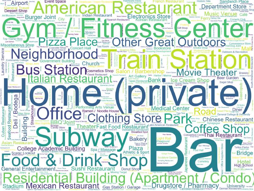
(b) weekday night

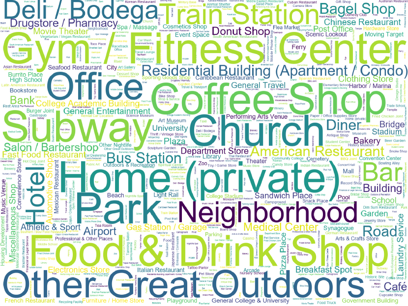
(c) weekend morning

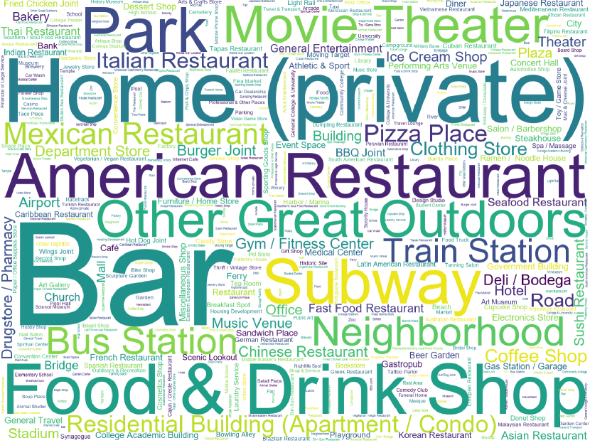
(d) weekend night

Figure 1. The illustrations of the periodic shift on points-of-interest (POI) dataset Foursquare-NYC, representing word clouds of POI for morning/night on weekdays/weekends.

Nonetheless, streaming recommendation confronts a significant challenge in the form of the phenomenon of time-varying user preferences (Ditzler et al., 2015). Users’ preferences change dynamically over time due to several factors such as seasonality, holidays, or circadian rhythm. As illustrated in Fig. 1, users tend to check in at places such as “Office” and “Coffee Shop” on weekday mornings, while at places like “Gym / Fitness Center” and “Church” on weekend mornings, demonstrating a weekly periodicity. In contrast to morning preferences, users tend to visit bars and spend time at home during evening hours regardless of whether it is a weekday or weekend, indicating a daily periodicity. Another interesting example of short video recommendation is that users exhibit a tendency to watch cartoons specifically on weekends, while preferring other types of content on weekdays. These recurring patterns highlight the importance of considering time-varying user preferences to avoid sub-optimal recommendations. Consequently, devising effective and efficient approaches to address the issue of users’ periodic time-varying preference is critical for achieving high-quality streaming recommendation.

As a classic framework for online learning, multi-armed bandit (MAB) algorithms have gained significant attention in recent years. A variation of MAB, known as contextual bandits (Langford and Zhang, 2007; Li et al., 2010; Wu et al., 2018), has achieved considerable success in various online services by utilizing both user feedback and contextual information related to users and items, which make it particularly advantageous in streaming recommendation scenarios. Most existing contextual bandit algorithms are constructed under stationary environment, i.e. users’ preferences remain static over time (Li et al., 2010; Balseiro et al., 2019; Han et al., 2020). However, the environment is always non-stationary in reality indicating time-varying user preferences. Some studies have noticed this problem and relaxed the assumption to the piecewise stationary environment (Wu et al., 2018; Xu et al., 2020), which enables algorithms to adaptively detect user preferences change points and discard learned model parameters for relearning. These approaches may result in performance fluctuations when handling periodic changes in user preferences. The primary reason is that these algorithms fail to recognize the periodic information of user preferences in an online manner and retrain the model even if the current period has occurred in the past. Currently, there is a notable research gap in the domain of streaming recommendations in periodic environments.

In this paper, we focus on a realistic environment setting where the reward function (i.e., the generation mechanism of user feedback) exhibits periodicity over time. Specifically, a large time period can be divided into multiple smaller periods in a periodic manner (e.g., based on the specific day of the week and different time slots within a day), and the reward function demonstrates a similar distribution whenever the same time period is encountered. Moreover, these time periods can be observed by the model and utilized for periodicity modeling and online adjustment of its user preference module in various streaming recommendation scenarios.

As a specific solution to the aforementioned process, we propose a novel contextual bandit algorithm called HyperBandit, which consists of two levels of model structures: 1). A bandit policy is designed to learn the latent features of items in an online fashion and combine them with the user preference matrix to execute online recommendations with effective exploration. 2). A hypernetwork takes the information of the time period as inputs and generates the parameters of the user preference matrix in the bandit policy. This hypernetwork captures the periodicity of user preferences over time and enables efficient online updating through low-rank factorization. The contributions are summarized as follows:

1. We propose a novel contextual bandit algorithm called HyperBandit, along with an efficient online training method utilizing low-rank factorization. HyperBandit explicitly models the periodic variations in user preferences and dynamically adjusts the recommendation policy based on time features.

2. We provide a sublinear regret guarantee for HyperBandit, ensuring the convergence of the online learning process. Additionally, we conduct empirical analysis on the low-rank structure in the parameter matrix, validating the rationale behind training via low-rank factorization.

3. We perform extensive experiments on various streaming recommendation tasks, including the recommendation of short videos and points of interest (POI), demonstrating the efficiency and effectiveness of the proposed HyperBandit algorithm.

2. Related Work

Hypernetworks (HNs) have been introduced by Ha et al. (Ha et al., 2016), drawing inspiration from the genotype-phenotype relation in cellular biology. HNs present an approach of using one network (hypernetwork) to generate weights for a second network (target network). In recent years, HNs are widely used in various domains such as computer vision (Klocek et al., 2019), language modeling (Suarez, 2017), sequence decoding (Nachmani and Wolf, 2019), continual learning  (von Oswald et al., 2020), federated learning (Shamsian et al., 2021), multi-objective optimization (Navon et al., 2021; Chen et al., 2023), and hyperparameter optimization (MacKay et al., 2019). Navon et al. (Navon et al., 2021) proposed a unified model to learn the Pareto front based on HNs that can be applied to a specific objective preference at inference time. von Oswald et al. (von Oswald et al., 2020) presented a task-aware method for continual model-based reinforcement learning using HNs, which allows the entire network to change between tasks as well as retaining performance on previous tasks. HNs have been widely applied in offline learning, but there is a lack of research on how to enhance the controllability of models through hypernetworks in online learning and streaming applications.

Bandits in non-stationary environment have attracted extensive attention in both theory and applications in recent years. One common setting for non-stationary environments is the abruptly changing or piecewise-stationary environment, where the environment undergoes sudden changes at unknown time points while remaining stationary between consecutive change points. Under the piecewise-stationary assumption, the problem has been well studied in the classical context-free setting (Hartland et al., 2006; Garivier and Moulines, 2008; Yu and Mannor, 2009; Slivkins and Upfal, 2008). Yu et al. (Yu and Mannor, 2009) proposed a windowed mean-shift detection algorithm to identify potential abrupt changes in the environment. They provided an upper bound on regret of $O\left(\Gamma_{T}\log(T)\right)$ for their algorithm, where $\Gamma_{T}$ represents the number of ground-truth changes up to time $T$. Within the contextual bandit setting, limited attention has been given to addressing non-stationary environments (Hariri et al., 2015; Wu et al., 2018; Xu et al., 2020). Wu et al. (Wu et al., 2018) developed a hierarchical bandit algorithm capable of detecting and adapting to changes by maintaining multiple contextual bandits. More recently, Xu et al. (Xu et al., 2020) addressed the challenge of time-varying preferences by employing a change-detection procedure to identify potential changes on the preference vectors. However, little attention has been given to addressing the issue of periodic reward drift that this paper focuses on.

3. Problem Formulation

3.1. Bandit-based Streaming Recommendation

Streaming recommendation can be formulated as a problem of sequential decision making, where the online service platform recommends the most relevant item $a\in\mathcal{A}$ (such as videos, music, or POIs) to a user $u\in\mathcal{U}$ in an online manner. Contextual bandit algorithms are well-suited for addressing streaming recommendation problems. More specifically, the candidate item set $\mathcal{A}$ could be viewed as the action space of the bandit algorithm, while the context space $\mathcal{S}$ summarizes the feature information of users and items, where each item $a$ and user $u$ can be associated with context feature vectors denoted by $\bm{c}_{a}$ and $\bm{c}_{u}$, respectively. At time step $t$, given a subset of the action space $\mathcal{A}_{t}\subseteq\mathcal{A}$ and a user, an item is selected by a recommendation policy and recommended to the user. After one item is recommended, the item may be clicked by the user (i.e, positive user feedback) or skipped (i.e, negative user feedback). Thereafter the true reward defined on the user feedback is received and could be used for updating the current recommendation policy, which will be adopted for the next recommendation.

The above process can be formalized as a contextual bandit problem for streaming recommendation, and represented using a 4-tuple $\left\langle\mathcal{A},\mathcal{S},\pi,r\right\rangle$:

Action space $\mathcal{A}$ denotes a given candidate action set, where each action (also called arm) corresponds to a specified candidate item. At each time step, a dynamic action space is selected as the candidate item set for recommendation. That is, at time step $t$, a candidate item set $\mathcal{A}_{t}\subseteq\mathcal{A}$ is recalled by some strategy, and choosing an action $a_{I_{t}}$ from $\mathcal{A}_{t}$ means that the corresponding item is recommended to the user, where $I_{t}\in|\mathcal{A}_{t}|$ denotes the index of the recommended item at time $t$.

Context space $\mathcal{S}$ summarizes the context feature information of users and items, denoted by $\bm{c}_{u}\in\mathbb{R}^{d_{u}}$ and $\bm{c}_{a}\in\mathbb{R}^{d_{a}}$, respectively. In this paper, in particular, we consider splitting the item context $\bm{c}_{a}\in\mathbb{R}^{d_{a}}$ into two parts: the observed features $\bm{s}_{a}\in\mathbb{R}^{o_{a}}$, and the latent features $\bm{x}_{a}\in\mathbb{R}^{l_{a}}$ that needs to be learned. Here, $\bm{c}_{a}=[\bm{s}_{a}^{\intercal},\bm{x}_{a}(t)^{\intercal}]^{\intercal}$ and the dimension of $\bm{c}_{a}$ is given by $d_{a}=o_{a}+l_{a}$.

Policy $\pi:\mathcal{S}\rightarrow\mathcal{A}$ describes the decision-making rule of an agent (i.e., the recommendation model), which selects an action for execution according to the relevance score of each action. at time $t$, given a candidate item set $\mathcal{A}_{t}$ and user $u\in\mathcal{U}$, a relevance score function $f_{t}$ treats context features of user and item in context space (i.e., $\bm{c}_{u}$ and $\bm{c}_{a}$ ) as inputs and determines which action to take: $a_{I_{t}}:=\arg\max_{a\in\mathcal{A}_{t}}f_{t}\left(\bm{c}_{u},\bm{c}_{a}\right)$.

Reward $r$ is defined upon the user feedback. Specifically, at time $t$, after recommending the item $a_{I_{t}}\in\mathcal{A}_{t}$ to a user $u$, a corresponding reward $r(u,a_{I_{t}})\in\{0,1\}$ is observed, which implicitly indicates whether the user feedback is negative or positive to the item $a_{I_{t}}$. However, the feedbacks from the same user towards the same item at different time may be quite different, which means that time-varying user preferences exist in it.

Table 1 summarizes the notations used throughout the paper.

Table 1. A summary of notations.

Symbol	Explanation
$[n]$	$[n]:=[1,2,\ldots,n]$
$t$	Time step $t\in[T]$
$\mathcal{A}$	Action space, i.e., the candidate item set
$|\mathcal{A}|$	The cardinality of set $\mathcal{A}$
$\bm{c}_{u}\in\mathbb{R}^{d_{u}}$	Context feature vector of a user $u$
$\bm{c}_{a}\in\mathbb{R}^{d_{a}}$	Context feature vector of a candidate item $a$
$\bm{s}_{a}\in\mathbb{R}^{o_{a}}$	Observed features of a candidate item $a$
$\bm{x}_{a}\in\mathbb{R}^{l_{a}}$	Latent features of a candidate item $a$
$p\in\mathcal{P}$	Time period variable, takes values in the range $\mathcal{P}:=\{0,1,\dots,34\}$, representing the 35 time periods within a week
$\bm{s}_{p}\in\mathbb{R}^{d_{p}}$	Time period embedding of time period $p$
$\bm{\Theta}_{p}^{*}$	True user preference matrix at the time period $p$

3.2. Time-Varying User Preferences

In this section, we formally describe the time-varying user preferences mentioned in the introduction.

As defined in Table 1, we first introduce the time period variable $p$ to measure specific temporal patterns, including hours of the day and different days of the week. Specifically, we divide a week into seven days, from Monday to Sunday, and further divide each day into the following five sessions: the morning (8:00 AM to 11:30 AM), the noon (11:30 AM to 2:00 PM), the afternoon (2:00 PM to 5:30 PM), the night (5:30 PM to 10:00 PM), and the remaining period. Then, the time period variable, $p$, encompasses 35 distinct values spanning from 0 to 34 in a sequential order. Each time period can be encoded to derive its respective time period embedding, denoted as $\bm{s}_{p}\in\mathbb{R}^{d_{p}}$.

Under the traditional assumption of a stationary environment, the mechanism of user feedback should be consistent at every time period. That is, the reward generation probability, represented as $\operatorname{Pr}\left\{r(u,a)=1\mid\bm{c}_{u},\bm{c}_{a}\right\}$, is assumed to remain constant across all time step $t\in[T]$. This implies that the level of preference that user $u$ has for the recommended item $a$ is independent of the specific time at which the recommendation is made. However, in real-world streaming recommender systems, users’ preferences change with time periodically, which has been observed in (Gao et al., 2013). For example, users usually visit office at weekday morning and bars at night. That is, the user feedback towards office may be different at different time period. In other words, given the context $\bm{c}_{u},\bm{c}_{a}$, the current time period $p$ and the corresponding time period embedding $\bm{s}_{p}$, the following inequality may hold:

(1) $$\operatorname{Pr}\left\{r(u,a)=1\mid\bm{c}_{u},\bm{c}_{a},\bm{s}_{p=i}\right\}\neq\operatorname{Pr}\left\{r(u,a)=1\mid\bm{c}_{u},\bm{c}_{a},\bm{s}_{p=j}\right\},$$

where $i\neq j$ and $i,j\in\left\{0,\dots,34\right\}$, and $\operatorname{Pr}\left\{r=1\mid\bm{c}_{u},\bm{c}_{a},\bm{s}_{p}\right\}$ denotes the time-varying reward generation probability indicating how much the user $u$ prefers the recommended item $a$ at time period $p$.

Formally, we can represent the observed reward generated by the time-varying reward generation probability as $r(u,a,p)$. Given a user $u$, a item $a$, and a time period $p$, the generation process of the observed reward can be formalized as $r(u,a,p):=r^{*}(u,a,p)+\eta$, where $r^{*}(u,a,p)$ represents the true reward, and $\eta$ is a random variable drawn from a distribution with zero mean. This additional error term $\eta$ captures the noise or uncertainty present in the observations. Clearly, we have the following expected reward:

$$\mathbb{E}[r(u,a,p)]=r^{*}(u,a,p)=\operatorname{Pr}\left\{r(u,a,p)=1\mid\bm{c}_{u},\bm{c}_{a},\bm{s}_{p}\right\}.$$

Next, we make specific assumptions about the form of the expected reward $\mathbb{E}[r(u,a,p)]$, i.e., the true reward. One straightforward approach is to concatenate the time period embedding with the context feature vectors. However, existing research (Galanti and Wolf, 2020) has shown that directly concatenating features from different spaces can make it difficult to capture meaningful information (i.e., time-varying information in this paper). To address this issue, we extend the existing linear expected reward in the contextual bandit setting by introducing the true user preference matrix $\bm{\Theta}_{p}^{*}$. Then, we can specify the true reward as the following time-varying true reward:

(2) $$r^{*}(u,a,p):=\bm{c}_{a}^{\intercal}\bm{\Theta}_{p}^{*}\bm{c}_{u},$$

where the true user preference matrix $\bm{\Theta}_{p}^{*}\in\mathbb{R}^{d_{a}\times d_{u}}$ is utilized to map the user contexts through a linear mapping, taking into account the time period $p$ as well as its embedding $\bm{s}_{p}$ as conditions. By applying this mapping, the resulting vector $\bm{\Theta}_{p}^{*}\bm{c}_{u}$ can effectively capture the time-varying user preferences across different time periods. In particular, when $d_{a}=d_{u}$ and $\bm{\Theta}_{p}^{*}$ is the identity matrix, the time-varying true reward degenerates to a fixed true reward in the traditional contextual bandit setting.

4. HyperBandit: The Proposed Algorithm

We propose a novel bandit algorithm tailored for periodic non-stationary streaming recommendation, called HyperBandit.

4.1. Algorithm Overview

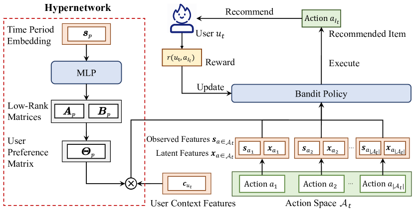
Figure 2. The structure of HyperBandit at time $t$.

Fig. 2 illustrates the structure of HyperBandit. Given the current time period as input, a hypernetwork generates a user preference matrix that maps user context features to a time-aware preference space. The mapped features, along with the item context features, are then utilized by the bandit policy to recommend a suitable item to the current user.

HyperBandit consists of the following two components. Firstly, it utilizes a bandit policy to update the latent features of items at each time step, enabling the preservation of time-varying latent features to capture distribution shifting. Secondly, it employs a hypernetwork that is trained in a mini-batch manner to adaptively adjust the user preference matrix in the bandit policy for a given time period. The algorithm’s detailed procedure is outlined in Algorithm 1. It’s important to note that the user preference matrix is estimated using two low-rank matrices during training. This specific training technique will be discussed in detail in Sec. 4.3.

4.2. Hypernetwork Assisted Bandit Policy

4.2.1. Bandit Policy using User Preference Matrix

To estimate the time-varying true reward and account for the user preference shift in each time period, we propose a novel bandit policy that utilizes an estimate of the true user preference matrix $\bm{\Theta}_{p}^{*}$ in Eq. (2). Specifically, the estimated user preference matrix, denoted as $\bm{\Theta}_{p}\in\mathbb{R}^{d_{a}\times d_{u}}$, captures the changes in user preferences during time period $p$. We estimate $\bm{\Theta}_{p}$ using a hypernetwork, which will be introduced in Sec. 4.2.2. The estimated user preference matrix allows us to adapt our bandit policy to the evolving user preferences. Formally, assuming that time step $t$ belongs to time period $p$, given a user context $\bm{c}_{u}\in\mathbb{R}^{d_{u}}$ and the estimated user preference matrix, the following ridge regression over the current interaction history is employed to estimate the item context $\bm{c}_{a}(t)$ at time $t\in[T]$:

(3) $$\bm{c}_{a}(t)=\operatornamewithlimits{arg\,min}\limits_{\bm{c}_{a}\in\mathbb{R}^{d_{a}}}\sum_{(u,a,r)\in\mathcal{H}_{t}}\left[\bm{c}_{a}^{\intercal}\bm{\Theta}_{p}\bm{c}_{u}-r(u,a,p)\right]^{2}+\lambda\|\bm{c}_{a}\|_{2}^{2},$$

where $\hat{r}_{u,a,p}:=\bm{c}_{a}^{\intercal}\bm{\Theta}_{p}\bm{c}_{u}$ denotes the estimated time-varying reward, $\mathcal{H}_{t}:=\left\{(u_{k},a_{I_{k}},r_{k})\right\}_{k\in[t]}$ represents the interaction history up to time $t$, $(u_{k},a_{I_{k}},r_{k})$ denotes that the policy recommended item $a_{I_{k}}$ to user $u_{k}$ at time $k$ and received a reward $r_{k}$, and $\lambda>0$ is the regularization parameter.

To reduce the uncertainty of user preference estimations, we introduce the observed item features. Specifically, we split the context $\bm{c}_{a}(t)$ at time $t$ of item $a\in\mathcal{A}_{t}$ into two parts, represented as $\bm{c}_{a}(t):=[\bm{s}_{a}^{\intercal},\bm{x}_{a}(t)^{\intercal}]^{\intercal}\in\mathbb{R}^{d_{a}}$, which includes: the observed features $\mathbf{s}_{a}\in\mathbb{R}^{o_{a}}$, and the latent features $\mathbf{x}_{a}(t)\in\mathbb{R}^{l_{a}}$ that needs to be learned online, where $d_{a}=o_{a}+l_{a}$. Accordingly, we redefine the estimated user preference matrix as $\bm{\Theta}_{p}=\left[\bm{\Theta}_{p}^{s\intercal},\bm{\Theta}_{p}^{x\intercal}\right]^{\intercal}$, where $\bm{\Theta}_{p}^{s}\in\mathbb{R}^{o_{a}\times d_{u}}$ corresponds to the observed item features $\bm{s}_{a}$, and $\bm{\Theta}_{p}^{x}\in\mathbb{R}^{l_{a}\times d_{u}}$ corresponds to the latent item features $\bm{x}_{a}(t)$. As a result, we can rewrite the ridge regression in Eq. (3) as follows:

(4) $$\hphantom{{}={}}\bm{x}_{a}(t)$$

$$=\operatornamewithlimits{arg\,min}\limits_{\bm{x}_{a}\in\mathbb{R}^{l_{a}}}\sum_{(u,a,r)\in\mathcal{H}_{t}}\left\{[\bm{s}_{a}^{\intercal},\bm{x}_{a}(t)^{\intercal}]\bm{\Theta}_{p}\bm{c}_{u}-r(u,a,p)\right\}^{2}+\lambda\|\bm{x}_{a}\|_{2}^{2}$$

$$=\operatornamewithlimits{arg\,min}\limits_{\bm{x}_{a}\in\mathbb{R}^{l_{a}}}\sum_{(u,a,r)\in\mathcal{H}_{t}}\left[\bm{s}_{a}^{\intercal}\bm{\Theta}_{p}^{s}\bm{c}_{u}+\bm{x}_{a}(t)^{\intercal}\bm{\Theta}_{p}^{x}\bm{c}_{u}-r(u,a,p)\right]^{2}+\lambda\|\bm{x}_{a}\|_{2}^{2}.$$

To solve the ridge regression Eq. (4), we can easily derive the closed-form solutions as $\bm{x}_{a,t}=\left(\bm{\Psi}_{a,t}\right)^{-1}\leavevmode\nobreak\ \bm{b}_{a,t}$, where

$$\bm{\Psi}_{a,t} =\sum_{u\in\mathcal{U}_{a,t}}\left(\bm{\Theta}_{p}^{x}\bm{c}_{u}\right)\left(\bm{\Theta}_{p}^{x}\bm{c}_{u}\right)^{\intercal}+\lambda\bm{I}_{l_{a}},$$

$$\bm{b}_{a,t} =\sum_{(u,a,r)\in\mathcal{H}_{t}}\bm{\left missing}(\bm{\Theta}_{p}^{x}\bm{c}_{u}\right)\left[r(u,a,p)-\left(\bm{\Theta}_{p}^{s}\bm{c}_{u}\right)^{\intercal}\bm{s}_{a}\right],$$

where $\mathcal{U}_{a,t}$ denotes the set of users (possibly with duplicates) who have been recommended item $a$ until time $t$, and $\bm{I}_{l_{a}}\in\mathbb{R}^{l_{a}\times l_{a}}$ is a identity matrix. The statistics $\left(\bm{\Psi}_{a,t},\bm{b}_{a,t}\right)$ can be updated incrementally and the detailed computation can be found in Algorithm 1.

According to the UCB policy in bandit algorithms (Li et al., 2010; Wang et al., 2017; Zhang et al., 2021), we define the following UCB-based relevance score function for executing action (i.e., online recommendation) at time $t$:

$$f_{t}(\bm{c}_{u},\bm{c}_{a}(t)):=\left[\bm{s}_{a}^{\intercal},\bm{x}_{a}(t)^{\intercal}\right]\bm{\Theta}_{p}\bm{c}_{u}+\alpha\left[\left(\bm{\Theta}_{p}^{x}\bm{c}_{u}\right)^{\intercal}\left(\bm{\Psi}_{a,t}\right)^{-1}\bm{\Theta}_{p}^{x}\bm{c}_{u}\right]^{\frac{1}{2}},$$

where $\alpha>0$ is the exploration parameter, and the term multiplied by $\alpha$ is the exploration term. In this way, the executed action at time $t$ can be selected by $a_{I_{t}}=\operatornamewithlimits{arg\,max}_{a\in\mathcal{A}_{t}}f_{t}(\bm{c}_{u},\bm{c}_{a}(t))$.

0:  Latent features of items $\bm{x}_{a\in\mathcal{A}}=\bm{0}^{l_{a}}$,data buffer $\mathcal{D}_{n=1}=\emptyset$, $\bm{\Phi}_{a\in\mathcal{A},t=1}=\bm{O}^{l_{a}\times l_{a}}$, $\bm{b}_{a\in\mathcal{A},t=1}=\bm{0}^{l_{a}}$, $\{T_{n}\}_{n\in[N]}$set of time steps in each updating part, regularization parameter $\lambda>0$, exploration parameter $\alpha>0$.

1:  Initialize hypernetwork parameters $\bm{\xi}_{n=1}$ with Xavier Normal

2:  for $n\in[N]$ do

3:     for $t=1$ to $T_{n}$ do

4:        Receive the user $u_{t}$ and the time period embedding $\bm{s}_{p_{t}}$

5:        Obtain the set of candidate items $\mathcal{A}_{t}$

6:        Obtain the observed features $\bm{s}_{a},\forall a\in\mathcal{A}_{t}$

7:        Obtain the latent features $\bm{x}_{a}(t),\forall a\in\mathcal{A}_{t}$

8:        Estimated the user preference matrix $\bm{\Theta}_{p_{t}}^{(n)}:=\left[\bm{\Theta}_{p_{t}}^{s(n)\intercal},\bm{\Theta}_{p_{t}}^{x(n)\intercal}\right]^{\intercal}\leftarrow h_{\bm{\xi}_{n}}(\bm{s}_{p_{t}})$

9:        Recommend item $a_{I_{t}}\in\mathcal{A}_{t}$ to user $u_{t}$ following $a_{I_{t}}\leftarrow\arg\max_{a\in\mathcal{A}_{t}}\left[\bm{s}_{a}^{\intercal},\bm{x}_{a}(t)^{\intercal}\right]\bm{\Theta}_{p_{t}}^{(n)}\bm{c}_{u_{t}}+\alpha\left[\left(\bm{\Theta}_{p_{t}}^{x(n)}\bm{c}_{u_{t}}\right)^{\intercal}\left(\bm{\Psi}_{a,t}\right)^{-1}\bm{\Theta}_{p_{t}}^{x(n)}\bm{c}_{u_{t}}\right]^{\frac{1}{2}}$

10:        Observe reward $r_{t}=r(u_{t},a_{I_{t}},p_{t})$

11:        $\mathcal{D}_{n}\leftarrow\mathcal{D}_{n}\cup\left\{(u_{t},a_{I_{t}},p_{t},r_{t},\mathcal{A}_{t})\right\}$

12:        $//\leavevmode\nobreak\ \leavevmode\nobreak\ \texttt{Bandit Policy Updating}$

13:        Get the user preference vector $\bm{P}_{t}\leftarrow\left(\bm{\Theta}_{p_{t}}^{x(n)}\bm{c}_{u_{t}}\right)^{\intercal}\in\mathbb{R}^{l_{a}}\leavevmode\nobreak\$ for the latent item features

14:        Get the user preference vector $\bm{Q}_{t}\leftarrow\left(\bm{\Theta}_{p_{t}}^{s(n)}\bm{c}_{u_{t}}\right)^{\intercal}\in\mathbb{R}^{o_{a}}$ for the observed item features

15:        $\bm{\Phi}_{a_{I_{t}},t+1}\leftarrow\bm{\Phi}_{a_{I_{t}},t}+\bm{P}_{t}^{\intercal}\bm{P}_{t}$,  $\bm{\Psi}_{a_{I_{t}},t+1}\leftarrow\lambda\bm{I}+\bm{\Phi}_{a_{I_{t}},t+1}$

16:        $\bm{b}_{a_{I_{t}},t+1}\leftarrow\bm{b}_{a_{I_{t}},t}+\bm{P}_{t}^{\intercal}\left(\bm{r}_{t}-\bm{Q}_{t}\bm{s}_{a_{I_{t}}}\right)$

17:        $\bm{x}_{a_{I_{t}},t+1}\leftarrow\left(\bm{\Psi}_{a_{I_{t}},t+1}\right)^{-1}\leavevmode\nobreak\ \bm{b}_{a_{I_{t}},t+1}$

18:     end for

19:     $//\leavevmode\nobreak\ \leavevmode\nobreak\ \texttt{ Hypernetwork Updating}$

20:     Update hypernetwork parameter $\bm{\xi}_{n+1}\leftarrow\Delta(\bm{\xi}_{n})$ using efficient training method via low-rank factorization (in Sec. 4.3.2) and the Adam optimizer on $\mathcal{D}_{n}$

21:     Release $\mathcal{D}_{n}$ and set $\mathcal{D}_{n+1}\leftarrow\emptyset$

22:  end for

Algorithm 1 HyperBandit

4.2.2. Hypernetwork for Time-Varying Preference

In the last section, we describe the bandit policy given parameter matrix $\bm{\Theta}_{p}$ in time period $p$. In this section, we explain how the hypernetwork generates the parameter matrix $\bm{\Theta}_{p}$. The main concept involves utilizing a hypernetwork that takes the embedding of the current time period as input and generates the parameters of the user preference matrix in the bandit policy. This enables the policy to adapt and adjust itself to accommodate changes in the distribution of user preferences over time.

To ensure stability in online recommendation, we incrementally update the hypernetwork $h$ in mini-batches, where the total $T$ time steps are divided into $N$ parts, and the $n$-th part, $n\in[N]$, contains $T_{n}$ time steps, corresponding to $T_{n}$ interaction histories. In this way, the hypernetwork $h$ is updated $N$ times, and during the $n$-th update, the data buffer $\mathcal{D}_{n}:=\left\{(u_{t},a_{I_{t}},p_{t},r_{t},\mathcal{A}_{t})\right\}_{t\in[T_{n}]}$ is used as the training data, where $r_{t}=r(u_{t},a_{I_{t}},p_{t})$. Then, given the time period embedding $\bm{s}_{p}$, the hypernetwork after the $(n-1)$-th update, denoted by $h_{\bm{\xi}_{n}}$, can be represented by:

(5) $$\bm{\Theta}_{p}^{(n)}:=h_{\bm{\xi}_{n}}(\bm{s}_{p}),$$

where $\bm{\xi}_{n}$ represents the model parameters of the hypernetwork, and the superscript $(n)$ on $\bm{\Theta}_{p}^{(n)}$ indicates that it is generated by $h_{\bm{\xi}_{n}}$. As illustrated in Figure 2, we implement the hypernetwork $h$ using a Multi-Layer Perceptron (MLP). In this way, the MLP acts like a condition network, inputting the embedding of current time period, outputting the corresponding user preference matrix. Besides, the time period embedding $\bm{s}_{p}$ is generated via GloVe model (Pennington et al., 2014) by imputing the current time period $p$.

To train the hypernetwork, we take inspiration from the Listnet loss design (Cao et al., 2007) to quantify the discrepancy between the estimated reward and the true label for each candidate item in $\mathcal{A}_{t}$ at time $t$. Specially, we use the estimated time-varying reward $\hat{r}_{u,a,p}=\bm{c}_{a}^{\intercal}\bm{\Theta}_{p}\bm{c}_{u}$ in Eq. (3), and construct the true labels according to the following rules: if the user $u$ clicks on the recommended item $a$ in time period $p$, the label is set to 1; if the user skips the recommended item, the label is set to -1; if the item is a candidate but not recommended, the label is set to 0. Formally, $y_{u,a,p}=1$ if $r_{u,a,p}=1$; $y_{u,a,p}=-1$ if $r_{u,a,p}$ = 0; $y_{u,a,p}=0$ if it is a candidate item but not recommended. Then, assuming that the number of actions is $M:=|\mathcal{A}_{1}|=\cdots=|\mathcal{A}_{T}|$, during the $n$-th incremental update, the loss function on the data buffer $\mathcal{D}_{n}$ could be shown as follows:

$$\mathcal{L}_{\bm{\xi}}^{(n)}=-\sum_{t=1}^{T_{n}}\sum_{k=1}^{M}P\left(y_{u_{t},a_{k},p_{t}}\right)\log\widehat{P}\left(\hat{r}_{u_{t},a_{k},p_{t}}\right),$$

where $\bm{\xi}$ represents the hypernetwork parameters that need to be optimized, $p_{t}$ corresponds to the time period where index $t$ in $\mathcal{D}_{n}$ is located, and

$$\widehat{P}\left(\hat{r}_{u_{t},a_{k},p_{t}}\right)=\frac{\exp\left(\hat{r}_{u_{t},a_{k},p_{t}}\right)}{\sum_{i=1}^{M}\exp\left(\hat{r}_{u_{t},a_{i},p_{t}}\right)},\leavevmode\nobreak\ {P}\left(y_{u_{t},a_{k},p_{t}}\right)=\frac{\exp\left(y_{u_{t},a_{k},p_{t}}\right)}{\sum_{i=1}^{M}\exp\left(y_{u_{t},a_{i},p_{t}}\right)}.$$

4.3. Efficient Training via Low-Rank Factorization

4.3.1. Analysis of Low-Rank Structure of User Preference Matrix

(a) KuaiRec

(b) NYC

(c) TKY

Figure 3. The distribution of singular eigenvalues (SEs) of user preference matrices across different time periods. The horizontal axis represents the index of SEs, arranged in descending order, while the vertical axis represents the time periods. The darkness of the colors corresponds to the magnitude of the singular values.

Since the user preference matrix $\bm{\Theta}_{p}\in\mathbb{R}^{d_{a}\times d_{u}}$ is generated by the hypernetwork in Eq. (5), a large output dimension (i.e., $d_{a}\times d_{u}$) would incur significant training costs. Hence, we consider representing the entire user preference matrix using a smaller number of parameters. Based on this motivation, it is natural to investigate whether the user preference matrix $\bm{\Theta}_{p}$ exhibits a low-rank structure. To verify the presence of low-rank structures, we perform singular value decomposition (SVD) on $\bm{\Theta}_{p}^{(N)}$ across different time periods. As shown in Fig. 3, when the singular values of the user preference matrices are sorted in descending order for different time periods, it becomes apparent that the distribution of singular values is concentrated in the first few dimensions, which is always less than half of the dimensionality of the user preference matrices. Based on this observation, we can conclude that there are strong low-rank structures present in the user preference matrices. This implies that a low-rank representation of the matrix $\bm{\Theta}_{p}$ could preserve nearly all of its information content.

4.3.2. Training Process with Low-Rank Factorization

Based on the analysis above, we try to improve the training efficiency of hypernetwork through explicitly modeling the low-rank structure in the user preference matrix $\bm{\Theta}_{p}$ (for ease of exposition, we omit the superscript of $\bm{\Theta}_{p}^{(n)}$ below). Specifically, we propose to approximate $\bm{\Theta}_{p}$ with its low-rank approximation. Here, we leverage matrix factorization approach to achieve the approximation. Given the estimated rank $\tau>0$, we model the low-rank structure of $\bm{\Theta}_{p}$ with the product of two rank-$\tau$ latent matrices $\bm{A}_{p}\in\mathbb{R}^{d_{a}\times\tau}$ and $\bm{B}_{p}\in\mathbb{R}^{d_{u}\times\tau}$, i.e., $\bm{\Theta}_{p}\approx\bm{A}_{p}\bm{B}_{p}^{\intercal}$, as shown in Fig. 4.

In the implementation of the hypernetwork, given a time period $p\in\mathcal{P}$, the hypernetwork outputs a vector represented by $\mathrm{Concat}(\mathrm{Vec}(\bm{A}_{p}),\mathrm{Vec}(\bm{B}_{p}))\in\mathbb{R}^{\tau d_{a}+\tau d_{u}}$, where $\mathrm{Concat}(\cdot)$ denotes the concatenation operation. Then, the vector $\mathrm{Vec}(\bm{A}_{p})\in\mathbb{R}^{\tau d_{a}}$ is reshaped into a matrix $\bm{A}_{p}\in\mathbb{R}^{d_{a}\times\tau}$, and the vector $\mathrm{Vec}(\bm{B}_{p})\in\mathbb{R}^{\tau d_{u}}$ is reshaped into a matrix $\bm{B}_{p}\in\mathbb{R}^{d_{u}\times\tau}$. Finally, the product $\bm{A}_{p}\bm{B}_{p}^{\intercal}$ is obtained to estimate $\bm{\Theta}_{p}$. This matrix factorization reduces the output dimension of the hypernetwork $h$ (defined in Eq. (5)) from $d_{a}d_{u}$ to $\tau(d_{a}+d_{u})$, effectively alleviating the training efficiency issues.

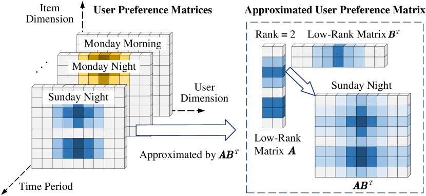
Figure 4. User preference matrix estimation using low rank factorization: An example with estimated rank $\tau=2$.

5. Regret Analysis

The regret bound serves as a fundamental theoretical guarantee for online learning algorithms (Cesa-Bianchi and Lugosi, 2006; Bubeck and Cesa-Bianchi, 2012; Shalev-Shwartz, 2011; Hazan, 2016; Zhang et al., 2019). In this section, we provide a regret bound of the proposed HyperBandit. First, we define the regret as follows:

(6) $$\mathrm{Reg}(T):=\sum_{t\in[T]}\left[r^{*}(u_{t},a_{t}^{*},p_{t})-r^{*}(u_{t},a_{I_{t}},p_{t})\right],$$

where $a_{t}^{*}$ represents the action with the highest time-varying true reward $r^{*}$ (defined in Eq. (2)) at time $t$, $u_{t}$ denotes the user for whom the item is recommended at time $t$, and $p_{t}$ represents the time period to which $t$ belongs. Recalling that $I_{t}$ denotes the index of the action executed by HyperBandit at time $t$, the regret in Eq. (6) measures the difference between the accumulated time-varying true rewards of the best policy and our policy.

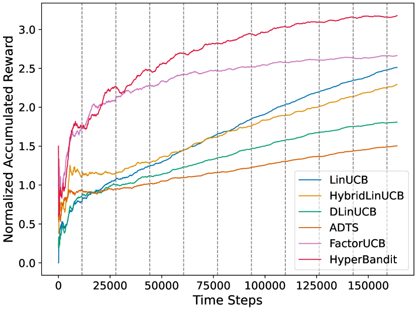
(a) KuaiRec

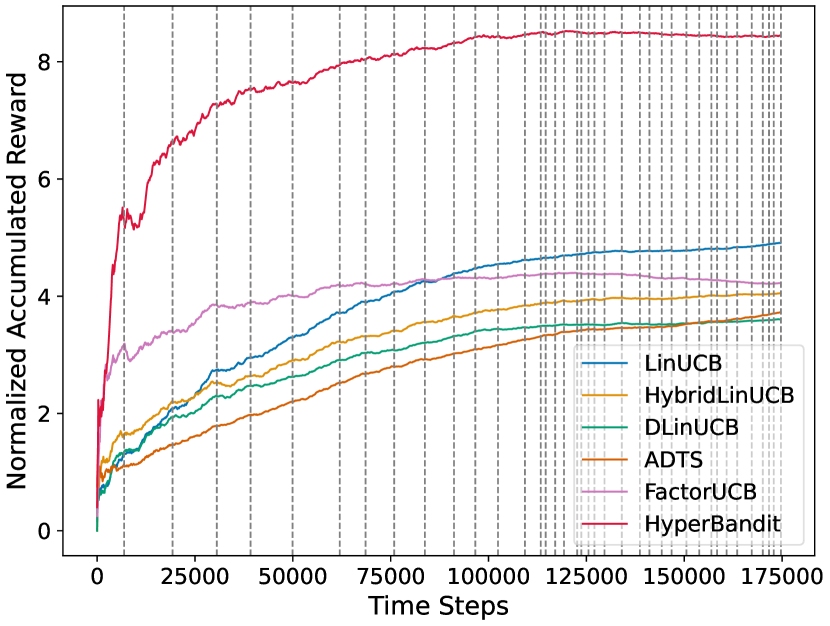
(b) NYC

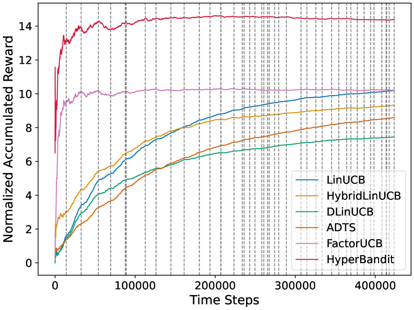
(c) TKY

Figure 5. Normalized accumulated reward of baselines, and the proposed HyperBandit on three datasets, KuaiRec & NYC & TKY. Note that The grey dashed lines represent the boundaries between weekdays and weekends. The $x$-axis represents the interaction data arranged in chronological order, and the $y$-axis represents the normalized accumulated reward.

Theorem 5.1 (Regret Upper Bound of HyperBandit).

Assume that the dimension of the latent features is $l_{a}=L,\forall a\in\mathcal{A}.$ The sequence of the actions executed by HyperBandit enjoys the following regret upper bound: with probability at least $1-\delta$,

(7) $$\mathrm{Reg}(T)\leq 2C_{\bm{x}}\sqrt{2LT\ln\left(1+\frac{C_{\bm{\Theta}}C_{\mathcal{U}}^{2}T}{2\lambda L\delta}\right)}+C_{\bm{x}}\sqrt{\frac{2}{\lambda}}\sum_{n\in[N]}E_{n},$$

where 1).  $C_{\bm{x}}=\max_{a\in\mathcal{A}_{T}}\|\bm{x}_{a}(T)-\bm{x}_{a}^{*}\|_{\bm{\Psi}_{a,T}}$, $\|\bm{x}\|_{\bm{\Psi}}:=\sqrt{\bm{x}^{\intercal}\bm{\Psi}\bm{x}}$ denotes the elliptic norm of $\bm{x}$ with respect to the matrix $\bm{\Psi}$, $\bm{x}_{a}^{*}$ is the true latent features of item $a$, and $C_{\bm{\Theta}}=\max_{n\in[N],p\in\mathcal{P}}\left\|\bm{\Theta}_{p}^{(n)}\right\|_{\mathrm{F}}^{2}$, $C_{\mathcal{U}}=\max_{u\in\mathcal{U}}\|\bm{c}_{u}\|_{2}^{2}$; 2).  $E_{n}:=\sum_{i\in[T_{n}]}\left\|\left(\bm{\Theta}_{p_{i,n}}^{(n)}-\bm{\Theta}_{p_{i,n}}^{*}\right)\bm{c}_{u_{i,n}}\right\|_{2}$ denotes the error caused by the hypernetwork updated $N$ times using $T_{n}$ examples in the $n$-th update, and the subscript $(\cdot)_{i,n}$ denotes the time step $i\in[T_{n}]$ after the $(n-1)$-th update.

The error $E_{n}$ in Eq. (7) caused by the hypernetwork can be decomposed into the sum of the following three parts. 1). Approximation error measures the discrepancy between the optimal hypothesis in hypernetwork space and the target function that generates $\bm{\Theta}_{p}^{*}\bm{c}_{u}$ in $E_{n}$. From the results in (Galanti and Wolf, 2020), we obtain that the approximation error of the hypernetwork $h$ (defined in Eq. (5)) with ReLU activation function is $\varepsilon$, providing that the number of trainable parameters in the hypernetwork is $\Omega\left(\varepsilon^{-U/S^{*}}+\varepsilon^{-P/S^{*}}\right)$, where we assume $d_{u}=U,\forall u\in\mathcal{U},$ $d_{p}=P,\forall p\in\mathcal{P}$, and $S^{*}$ denotes the order of smoothness of the target function. 2). Optimization error: measures the accumulated deviation between the hypernetwork parameters obtained through the online optimization algorithm and those of the optimal hypothesis in the hypernetwork space. Our HyperBandit equipped with a mini-batch first-order optimization method incurs an accumulated optimization error of order $O(T/N)$, assuming that each data buffer $\mathcal{D}_{n},n\in[N]$ contains an equal number of examples. 3). Estimation error measures the the error caused by the estimated user preference matrix using low-rank factorization. According to the analyses in Sec. 4.3.1, the user preference matrix exhibits a low-rank structure. Assuming that the maximum rank of the user preference matrices is $R$, if the estimated rank $\tau$ in the low-rank factorization discussed in Sec. 4.3.2 is set to $\tau\geq R$, and the best rank-$\tau$ approximation can be obtained, then the estimation error would be zero.

Setting the number of trainable parameters in the hypernetwork as $\Omega\left(\sqrt{T}^{U/S^{*}}+\sqrt{T}^{P/S^{*}}\right)$, the number of hypernetwork training iterations $N=O(\sqrt{T})$, and the estimated rank $\tau\geq R$, we can derive an upper bound for the error term $\sum_{n\in[N]}E_{n}$ in Eq. (7) of order $\widetilde{O}(\sqrt{T})$. This, in turn, leads to a sublinear regret upper bound of order $\widetilde{O}(\sqrt{T})$ for HyperBandit.

6. Experiments

We conducted experiments to evaluate the performance of HyperBandit on datasets for short video recommendation and point-of-interest (POI) recommendation.

Table 2. Comparisons of normalized accumulated reward, running time (sec., mean) and training time (sec., mean) of hypernetwork on KuaiRec, Foursquare (NYC) and Foursquare (TKY). The “Running Time of BP” means the average time cost of online recommendation and updating by Bandit Policy at each time step, and the “Training Time of HN” means the average time cost for training HyperNetwork at each time step. “–” means the corresponding algorithm has no hypernetwork.

Algorithm	Normalized Accumulated Reward			Running Time of BP		Training Time of HN
	KuaiRec	NYC	TKY	KuaiRec	Foursquare	KuaiRec	Foursquare
LinUCB	$2.56\pm 0.04$	$4.86\pm 0.05$	$10.15\pm 0.10$	$3.09\mathrm{e-}04$	$3.08\mathrm{e-}04$	–	–
HybridLinUCB	$2.29\pm 0.03$	$4.05\pm 0.07$	$9.33\pm 0.03$	$2.52\mathrm{e-}02$	$2.65\mathrm{e-}02$	–	–
DLinUCB	$1.84\pm 0.03$	$3.63\pm 0.08$	$7.39\pm 0.08$	$3.51\mathrm{e-}04$	$3.55\mathrm{e-}04$	–	–
ADTS	$1.50\pm 0.02$	$3.80\pm 0.10$	$8.63\pm 0.09$	$6.52\mathrm{e-}03$	$6.69\mathrm{e-}03$	–	–
FactorUCB	$2.70\pm 0.05$	$4.19\pm 0.04$	$10.22\pm 0.03$	$1.01\mathrm{e-}01$	$1.11\mathrm{e-}01$	–	–
HyperBandit ($\tau=1$)	$\mathbf{3.79\pm 0.18}$	$6.46\pm 0.45$	$13.37\pm 0.22$	$1.65\mathrm{e-}03$	$1.62\mathrm{e-}03$	$1.45\mathrm{e-}04$	$1.06\mathrm{e-}04$
HyperBandit ($\tau=5$)	$3.51\pm 0.06$	$8.08\pm 0.09$	$13.99\pm 0.29$	$1.60\mathrm{e-}03$	$1.63\mathrm{e-}03$	$1.58\mathrm{e-}04$	$1.21\mathrm{e-}04$
HyperBandit w/o Low-Rank	$3.24\pm 0.11$	$\mathbf{8.27\pm 0.17}$	$\mathbf{14.49\pm 0.07}$	$1.63\mathrm{e-}03$	$1.62\mathrm{e-}03$	$1.72\mathrm{e-}04$	$1.73\mathrm{e-}04$

6.1. Experimental Settings

6.1.1. Baselines.

HyperBandit was compared with several algorithms that construsted in stationary or piecewise-stationary environment, including:

LinUCB (Li et al., 2010) is a classical contextual bandit algorithm that addresses the problem of personalized recommendation.

HybridLinUCB (Li et al., 2010) is a variant algorithm of LinUCB that takes into account both shared and non-shared interests among users.

DLinUCB (Wu et al., 2018) is built upon a piecewise stationary environment, where each user group corresponds to a slave model. Whether to discard a slave model is based on the detection of “badness”.

ADTS (Hariri et al., 2015) is a bandit algorithm based on Thompson sampling, which tend to discard parameters before the last change point.

FactorUCB (Wang et al., 2017) leverages observed contextual features and user interdependencies to improve the convergence rate and help conquer cold-start in recommendation.

6.1.2. Hyperparameter Settings.

We implemented the hypernetwork $h$ in Eq. (5) using a MLP. The MLP consists of 1 input layer, 8 hidden layers, and 1 output layer. The number of nodes in the each layer is as follows: 30, 256, 512, 1024, 1024, 1024, 1024, 512, 256, $25*\tau*2$. We applied ReLU activation function after each hidden layer. We trained the hypernetwork every 2000 time steps (i.e., $T_{n}=2000,n\in[N]$) on KuaiRec and NYC, while $T_{n}=5000$ on TKY. Early stopping is applied in training process to avoid overfitting.

For the parameters in bandit policy, we set the exploration parameter $\alpha$ to 0.1 and the regularization parameter $\lambda$ to 0.1 for all the algorithms. The size of the candidate item set $\mathcal{A}_{t},\forall t\in[T]$ at each time step was set to 25 in all algorithms. The dimensions of both the context features of users and the context features of items were set to 25. In FactorUCB and HyperBandit, the dimensions of latent features of items were set to 10, and the dimensions of observed features of items were set to 15.

6.1.3. Evaluation Protocol.

The accumulated reward was utilized to assess the recommendation accuracy of algorithms, which was computed as the sum of the observed reward from the beginning to the current step. The normalized accumulated reward refers to the accumulated reward normalized by the corresponding logged random strategy.

6.2. Experiments on Short Video Recommendation

We employed KuaiRec (Gao et al., 2022) for evaluation, that is a real-world dataset collected from the recommendation logs of the video-sharing mobile app Kwai. The dense interaction matrix we used contains 1411 users, 3327 items and 529 video categories (i.e., tags). Each interactive data includes user id, video id, play duration, video duration, time, date, timestamp, and watch ratio, etc. Following the settings in (Wan et al., 2021), we used video categories (tags) as actions. In this experiment, we treated watch ratio higher than 2.0 as positive feedback. If the action (i.e., tag) got positive feedback in other time periods while not in current period, we assumed that the current user would give a negative feedback to it.

To fit the data into the contextual bandit setting, we pre-processed it first. Initially, we encoded all the user features provided by KuaiRec, including user activity level, number of followed users, and others. Subsequently, we applied PCA to reduce the dimensionality of the context feature vectors. We retained the first 25 principal components and applied the same procedure to the context feature vectors of items (i.e., $d_{a}=d_{u}=25$ ). For a particular time step, the video tag id having positive feedback was picked and the remaining 24 were randomly sampled from the tags which would get negative feedback in the current time step. Besides, we extracted data for one week from August 10th, 2020, to August 16th, 2020. From each time period within that week, we randomly sampled several time steps to reconstruct the data. This sampling process was repeated 10 times to generate data for 10 weeks.

The results are shown in Fig. 5(a) and Table 2, we can clearly notice that HyperBandit outperformed all the other baselines on KuaiRec in terms of rewards. As environment is periodic, both DLinUCB and ADTS were worse than others since these two algorithms were designed for the piece-wise stationary environment (i.e., they need to abandon the knowledge acquired during past periods). As more observations recurrent, LinUCB quickly catched up, because it is better to regard periodic environment as a stationary environment rather than piecewise environment. Besides, FactorUCB leveraged observed contextual features and dependencies among users to improve the algorithm’s convergence rate, leading to good performance at the beginning.

6.3. Experiments on POI Recommendation

Foursquare NYC & TKY dataset (Yang et al., 2015) includes long-term (about 10 months) check-in data in New York city (NYC) and Tokyo (TKY) collected from Foursquare from 12 April 2012 to 16 February 2013. Table 3 shows the statistics of two check-in datasets: NYC and TKY. Each dataset includes user id, venue id, venue category id, venue category name, latitude, longitude, and timestamp, etc.

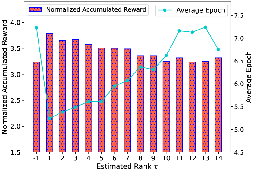
(a) KuaiRec

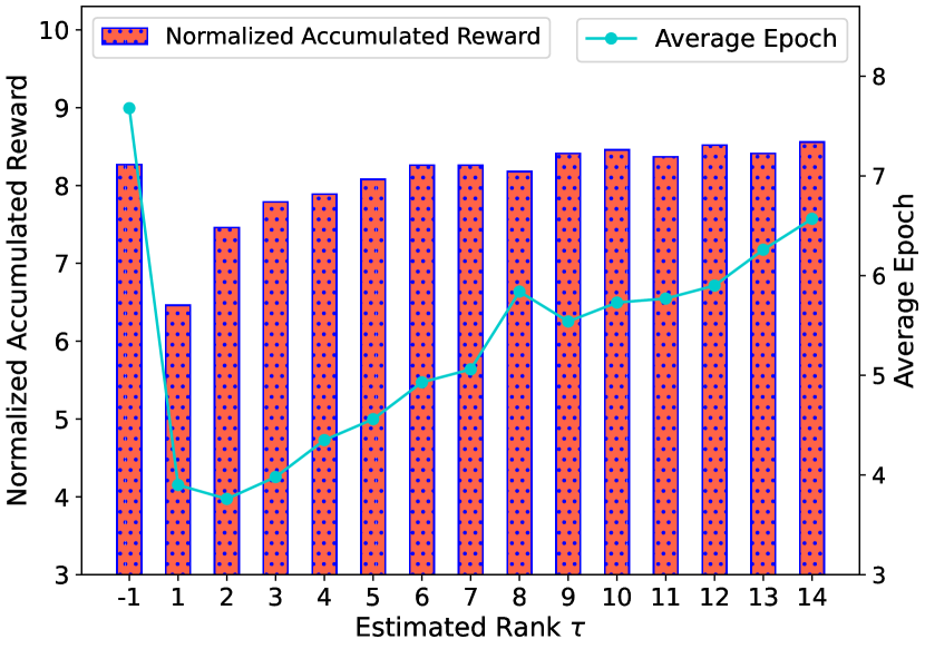
(b) NYC

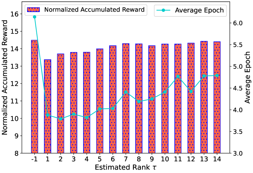
(c) TKY

Figure 6. Performance of low-rank factorization in HyperBandit on different estimated rank across three datasets. Note that the bar chart shows normalized accumulated reward, while the line chart shows average epoch in training process (a larger average epoch indicates a longer training time of hypernetwork). The first data point (with an $x$-coordinate of “$\mathrm{-1}$”) represents the result obtained without utilizing low-rank factorization.

Similarly, we used POI categories as actions. The ground-truth categories of the check-ins were considered positive samples of the current step while the rest categories were considered negative. Initially, instead of following the setting in (Cesa-Bianchi et al., 2013) that used TF-IDF for representation construction, we employed the GloVe model (Pennington et al., 2014) to craft a 300-dimensional feature vector, enhancing item context representation. Subsequently, PCA reduced vector dimensionality, retaining the initial 25 principal components. Since these two datasets do not contain user profiles, we used the interaction data from the first week to construct the contextual features of users. Specifically, we used the average vector of all the POI category feature vectors that the user checked in during the first week as the user context feature vector. For the candidate action set at each time step, we selected the ground-truth check-in tag and randomly extracted 24 negative categories of the current step. We used all the data from April 10th, 2012 to February 16th, 2013 (except data from the first week) to construct a data streaming.

Table 3. The statistics of the Foursquare NYC & TKY.

Dataset	#Users	#POIs	#POI Categories	#Check-ins
NYC	1,083	38,333	400	227,428
TKY	2,293	61,858	385	573,703

As illustrated in Fig. 5(b) and Fig. 5(c), similar conclusions can be drawn as in KuaiRec. Additionally, we conducted an analysis of time cost for all algorithms and compared the performance of different estimated rank ($\tau=1$, $\tau=5$ and w/o Low-Rank) of HyperBandit. The corresponding results are presented in Table 2. Notably, HyperBandit consistently outperformed the baselines in terms of normalized accumulated reward, while the running time of BP (bandit policy) remained acceptable. FactorUCB achieved excellent performance among baselines due to leveraging user adjacency relationships. However, that also lead to a significant time cost as FactorUCB required updating all user parameters at each time step. Furthermore, HyperBandit ($\tau=1$) and HyperBandit ($\tau=5$) reduced the training time of HN by 15.7%, 8.1% in KuaiRec and 38.7%, 30.1% on Foursquare dataset compared to HyperBandit (w/o Low-Rank), which provided strong evidences of the training efficiency with low-rank factorization.

6.4. Ablation Experiments

In this section, we empirically studied the proposed HyperBandit by addressing the following research questions:

RQ1: Is HyperBandit efficient enough to meet the real-time requirements of online recommendations?

RQ2: How does the estimated rank $\tau$ of low-rank factorization affect HyperBandit?

RQ3: What is the impact of key components in HyperBandit on the recommendation performance?

6.4.1. RQ1: Running Time

In streaming recommendation scenarios, running time is another important metric. We reports the running time of bandit policy and the training time of hypernetwork in Table 2. From the results, we conclude that the time cost of HyperBandit was on the order of milliseconds (ms), indicating that HyperBandit met the real-time requirements in streaming recommendations. Furthermore, the training time of the hypernetwork exhibits a decreasing trend as the estimated rank $\tau$ decreases from full rank to $1$, validating its efficiency in low-rank updating.

6.4.2. RQ2: Impact of Estimated Rank $\tau$

Fig. 6 explored the impact of different estimated rank of low-rank factorization on the performance in terms of normalized accumulated reward and training time. The observations from the experimental results can be summarized as follows: 1). With an increase in the estimated rank $\tau$, our HyperBandit demonstrated an overall improvement in normalized accumulated reward on Foursquare datasets, and the normalized accumulated reward of HyperBandit with ranks ranging from 2 to 14 were nearly equivalent to that of HyperBandit without low-rank factorization. Particularly on KuaiRec dataset, HyperBandit with ranks from 1 to 9 even outperformed the algorithm without low-rank factorization. These results validate the effectiveness of the low-rank factorization approach, which maintains excellent performance. 2). The average epoch, which measures the training time of the hypernetwork, also exhibits an overall upward trend as the estimated rank $\tau$ increases, although it is significantly smaller than that without low-rank factorization. This observation highlights the benefits of efficient training via low-rank factorization as described in Sec. 4.3.2.

6.4.3. RQ3: Impact of Key Components in HyperBandit.

HyperBandit consists of two key components for online updating: one is to update the latent features of items via ridge regression, and the other is to update the parameters of the hypernetwork through gradient descent. To investigate the interplay between these two updating components, an ablation experiment was conducted with the following settings: 1). Disable ridge regression updating: The dimension of the latent item features was set to zero. 2). Disable hypernetwork updating: The hypernetwork parameters were frozen to their initial state. The results are presented in Table 4. Based on the results, the following conclusions can be drawn: 1). Employing both updating components independently enhances the recommendation performance. 2). Irrespective of whether ridge regression was enabled or disabled, the utilization of the hypernetwork can lead to performance improvements.

Table 4. The results of the ablation experiment on key components of HyperBandit. Note that the ridge regression updating in the bandit policy is denoted by “RR”, and the hypernetwork updating is referred to as “HN”. The symbol ✓  signifies the inclusion of a particular update process, while the symbol ✗  indicates its exclusion.

RR	HN	Normalized Accumulated Reward
		KuaiRec	NYC	TKY
✗	✗	$0.93\pm 0.08$	$0.87\pm 0.08$	$1.14\pm 0.44$
✓	✗	$1.09\pm 0.08$	$5.62\pm 0.52$	$13.26\pm 0.23$
✗	✓	$1.86\pm 0.09$	$4.90\pm 0.28$	$10.91\pm 0.35$
✓	✓	$\mathbf{3.24\pm 0.11}$	$\mathbf{8.27\pm 0.17}$	$\mathbf{14.49\pm 0.07}$

7. Conclusion

This paper aims to model the user preference shift in periodic non-stationary streaming recommendation scenarios. Specifically, we propose an online learning approach called HyperBandit. The proposed HyperBandit leverages a hypernetwork to dynamically adjust user preference parameters for estimating time-varying rewards, employs a bandit policy for online recommendation with a regret guarantee, and utilizes a low-rank factorization method to efficiently train the model. Experimental results demonstrated the effectiveness and efficiency of HyperBandit in steaming recommendation. The proposed HyperBandit has opened up a promising avenue for advancing controllable online learning.

References

- (1)
- Balseiro et al. (2019) Santiago Balseiro, Negin Golrezaei, Mohammad Mahdian, Vahab Mirrokni, and Jon Schneider. 2019. Contextual Bandits with Cross-Learning. In Advances in Neural Information Processing Systems 32. 9679–9688.
- Bubeck and Cesa-Bianchi (2012) Sébastien Bubeck and Nicolò Cesa-Bianchi. 2012. Regret Analysis of Stochastic and Nonstochastic Multi-armed Bandit Problems. Journal of Foundations and Trends® in Machine Learning 5 (2012), 1–122.
- Cao et al. (2007) Zhe Cao, Tao Qin, Tie-Yan Liu, Ming-Feng Tsai, and Hang Li. 2007. Learning to rank: from pairwise approach to listwise approach. In Proceedings of the 24th International Conference on Machine learning. 129–136.
- Cesa-Bianchi et al. (2013) Nicolo Cesa-Bianchi, Claudio Gentile, and Giovanni Zappella. 2013. A gang of bandits. (2013), 2265–2279.
- Cesa-Bianchi and Lugosi (2006) Nicolò Cesa-Bianchi and Gabor Lugosi. 2006. Prediction, learning, and games. Cambridge University Press.
- Chandramouli et al. (2011) Badrish Chandramouli, Justin J Levandoski, Ahmed Eldawy, and Mohamed F Mokbel. 2011. Streamrec: A real-time recommender system. In Proceedings of the 2011 ACM SIGMOD International Conference on Management of Data. 1243–1246.
- Chang et al. (2017) Shiyu Chang, Yang Zhang, Jiliang Tang, Dawei Yin, Yi Chang, Mark A Hasegawa-Johnson, and Thomas S Huang. 2017. Streaming Recommender Systems. In Proceedings of the 26th International Conference on World Wide Web. 381–389.
- Chen et al. (2023) Sirui Chen, Yuan Wang, Zijing Wen, Zhiyu Li, Changshuo Zhang, Xiao Zhang, Quan Lin, Cheng Zhu, and Jun Xu. 2023. Controllable Multi-Objective Re-ranking with Policy Hypernetworks. In Proceedings of the 29th ACM SIGKDD Conference on Knowledge Discovery and Data Mining. 3855–3864.
- Ditzler et al. (2015) Gregory Ditzler, Manuel Roveri, Cesare Alippi, and Robi Polikar. 2015. Learning in nonstationary environments: A survey. Journal of IEEE Computational Intelligence Magazine 10 (2015), 12–25.
- Galanti and Wolf (2020) Tomer Galanti and Lior Wolf. 2020. On the modularity of hypernetworks. (2020), 10409–10419.
- Gao et al. (2022) Chongming Gao, Shijun Li, Wenqiang Lei, Jiawei Chen, Biao Li, Peng Jiang, Xiangnan He, Jiaxin Mao, and Tat-Seng Chua. 2022. KuaiRec: A Fully-Observed Dataset and Insights for Evaluating Recommender Systems. In Proceedings of the 31st ACM International Conference on Information & Knowledge Management. 540–550.
- Gao et al. (2013) Huiji Gao, Jiliang Tang, Xia Hu, and Huan Liu. 2013. Exploring temporal effects for location recommendation on location-based social networks. In Proceedings of the 7th ACM conference on Recommender Systems. 93–100.
- Garivier and Moulines (2008) Aurélien Garivier and Eric Moulines. 2008. On upper-confidence bound policies for non-stationary bandit problems. arXiv preprint arXiv:0805.3415 (2008).
- Ha et al. (2016) David Ha, Andrew Dai, and Quoc V Le. 2016. Hypernetworks. arXiv preprint arXiv:1609.09106 (2016).
- Han et al. (2020) Yanjun Han, Zhengqing Zhou, Zhengyuan Zhou, Jose Blanchet, Peter W Glynn, and Yinyu Ye. 2020. Sequential batch learning in finite-action linear contextual bandits. arXiv preprint arXiv:2004.06321 (2020).
- Hariri et al. (2015) Negar Hariri, Bamshad Mobasher, and Robin Burke. 2015. Adapting to user preference changes in interactive recommendation. In Proceedings of the 24th International Joint Conference on Artificial Intelligence. 4268–4274.
- Hartland et al. (2006) C. Hartland, S. Gelly, N. Baskiotis, O. Teytaud, and M. Sebag. 2006. Multi-armed Bandit, Dynamic Environments and Meta-Bandits. (2006).
- Hazan (2016) Elad Hazan. 2016. Introduction to online convex optimization. Journal of Foundations and Trends® in Optimization 2 (2016), 157–325.
- Jakomin et al. (2020) Martin Jakomin, Zoran Bosnic, and Tomaz Curk. 2020. Simultaneous Incremental Matrix Factorization for Streaming Recommender Systems. Journal of Expert Systems with Applications 160 (2020), 113685.
- Klocek et al. (2019) Sylwester Klocek, Łukasz Maziarka, Maciej Wołczyk, Jacek Tabor, Jakub Nowak, and Marek Śmieja. 2019. Hypernetwork functional image representation. In Proceedings of 28th International Conference on Artificial Neural Networks. 496–510.
- Langford and Zhang (2007) John Langford and Tong Zhang. 2007. The epoch-greedy algorithm for contextual multi-armed bandits. (2007), 96–1.
- Li et al. (2010) Lihong Li, Wei Chu, John Langford, and Robert E Schapire. 2010. A contextual-bandit approach to personalized news article recommendation. In Proceedings of the 19th International Conference on World Wide Web. 661–670.
- MacKay et al. (2019) Matthew MacKay, Paul Vicol, Jon Lorraine, David Duvenaud, and Roger Grosse. 2019. Self-tuning networks: Bilevel optimization of hyperparameters using structured best-response functions. arXiv preprint arXiv:1903.03088 (2019).
- Nachmani and Wolf (2019) Eliya Nachmani and Lior Wolf. 2019. Hyper-graph-network decoders for block codes. (2019), 2326–2336.
- Navon et al. (2021) Aviv Navon, Aviv Shamsian, Ethan Fetaya, and Gal Chechik. 2021. Learning the Pareto Front with Hypernetworks. In Proceedings of the 9th International Conference on Learning Representations.
- Pennington et al. (2014) Jeffrey Pennington, Richard Socher, and Christopher D Manning. 2014. Glove: Global vectors for word representation. In Proceedings of the 2014 Conference on Empirical Methods in Natural Language Processing. 1532–1543.
- Shalev-Shwartz (2011) Shai Shalev-Shwartz. 2011. Online learning and online convex optimization. Journal of Foundations and Trends® in Machine Learning 4 (2011), 107–194.
- Shamsian et al. (2021) Aviv Shamsian, Aviv Navon, Ethan Fetaya, and Gal Chechik. 2021. Personalized federated learning using hypernetworks. In Proceedings of the 38th International Conference on Machine Learning. 9489–9502.
- Slivkins and Upfal (2008) Aleksandrs Slivkins and Eli Upfal. 2008. Adapting to a Changing Environment: the Brownian Restless Bandits.. In COLT. 343–354.
- Suarez (2017) Joseph Suarez. 2017. Language modeling with recurrent highway hypernetworks. Advances in neural information processing systems 30 (2017), 3267–3276.
- von Oswald et al. (2020) Johannes von Oswald, Christian Henning, João Sacramento, and Benjamin F. Grewe. 2020. Continual learning with hypernetworks. In Proceedings of the 8th International Conference on Learning Representations.
- Wan et al. (2021) Yongquan Wan, Junli Xian, and Cairong Yan. 2021. A Contextual Multi-armed Bandit Approach Based on Implicit Feedback for Online Recommendation. In Proceedings of the 15th Knowledge Management in Organizations. 380–392.
- Wang et al. (2017) Huazheng Wang, Qingyun Wu, and Hongning Wang. 2017. Factorization bandits for interactive recommendation. In Proceedings of the AAAI Conference on Artificial Intelligence.
- Wang et al. (2018a) Qinyong Wang, Hongzhi Yin, Zhiting Hu, Defu Lian, Hao Wang, and Zi Huang. 2018a. Neural memory streaming recommender networks with adversarial training. In Proceedings of the 24th ACM SIGKDD International Conference on Knowledge Discovery & Data Mining. 2467–2475.
- Wang et al. (2018b) Weiqing Wang, Hongzhi Yin, Zi Huang, Qinyong Wang, Xingzhong Du, and Quoc Viet Hung Nguyen. 2018b. Streaming ranking based recommender systems. In Proceedings of the 41st International ACM SIGIR Conference on Research & Development in Information Retrieval. 525–534.
- Wu et al. (2018) Qingyun Wu, Naveen Iyer, and Hongning Wang. 2018. Learning contextual bandits in a non-stationary environment. In Proceedings of the 41st International ACM SIGIR Conference on Research & Development in Information Retrieval. 495–504.
- Xu et al. (2020) Xiao Xu, Fang Dong, Yanghua Li, Shaojian He, and Xin Li. 2020. Contextual-bandit based personalized recommendation with time-varying user interests. In Proceedings of the AAAI Conference on Artificial Intelligence. 6518–6525.
- Yang et al. (2015) Dingqi Yang, Daqing Zhang, Vincent. W. Zheng, and Zhiyong Yu. 2015. Modeling User Activity Preference by Leveraging User Spatial Temporal Characteristics in LBSNs. Journal of IEEE Transactions on Systems, Man, and Cybernetics: Systems 45 (2015), 129–142.
- Yu and Mannor (2009) Jia Yuan Yu and Shie Mannor. 2009. Piecewise-stationary bandit problems with side observations. In Proceedings of the 26th Annual International Conference on Machine Learning. 1177–1184.
- Zhang et al. (2022) Xiao Zhang, Sunhao Dai, Jun Xu, Zhenhua Dong, Quanyu Dai, and Ji-Rong Wen. 2022. Counteracting user attention bias in music streaming recommendation via reward modification. In Proceedings of the 28th ACM SIGKDD Conference on Knowledge Discovery and Data Mining. 2504–2514.
- Zhang et al. (2021) Xiao Zhang, Haonan Jia, Hanjing Su, Wenhan Wang, Jun Xu, and Ji-Rong Wen. 2021. Counterfactual reward modification for streaming recommendation with delayed feedback. In Proceedings of the 44th International ACM SIGIR Conference on Research and Development in Information Retrieval. 41–50.
- Zhang et al. (2019) Xiao Zhang, Yun Liao, and Shizhong Liao. 2019. A survey on online kernel selection for online kernel learning. WIREs Data Mining and Knowledge Discovery 9 (2019), e1295.