Episodic Bayesian Optimal Control with Unknown Randomness Distributions

Abstract

Stochastic optimal control with unknown randomness distributions has been studied for a long time, encompassing robust control, distributionally robust control, and adaptive control. We propose a new episodic Bayesian approach that incorporates Bayesian learning with optimal control. In each episode, the approach learns the randomness distribution with a Bayesian posterior and subsequently solves the corresponding Bayesian average estimate of the true problem. The resulting policy is exercised during the episode, while additional data/observations of the randomness are collected to update the Bayesian posterior for the next episode. We show that the resulting episodic value functions and policies converge almost surely to their optimal counterparts of the true problem if the parametrized model of the randomness distribution is correctly specified. We further show that the asymptotic convergence rate of the episodic value functions is of the order $O(N^{-1/2})$. We develop an efficient computational method based on stochastic dual dynamic programming for a class of problems that have convex value functions. Our numerical results on a classical inventory control problem verify the theoretical convergence results and demonstrate the effectiveness of the proposed computational method.

Keywords stochastic optimal control  $\cdot$ Bayesian learning  $\cdot$ stochastic dual dynamic programming

1 Introduction

Stochastic Optimal Control (SOC) provides a principled approach to dynamic decision making under uncertainty. It models the transition of the system state with a dynamic equation driven by randomness, with the assumption that the distribution of randomness is known. However, in practical problems, modeling randomness frequently depends on pre-collected data or observations, which introduces uncertainty regarding the distribution of randomness. This type of model uncertainty is also referred to as Knightian uncertainty or epistemic uncertainty in the literature.

There has been a long history of efforts to address this model uncertainty in stochastic optimal control, ranging from robust control to the recently developed distributionally robust control. Robust control (e.g., [6][17][8]), closely related to minimax control and $H^{\infty}$ control (e.g., [7][1]), often models the control problem as a game between the decision maker and nature, where nature selects the worst-case scenario in the uncertainty set while the decision maker aims to find the optimal control in the worst-case scenario. Depending on whether the uncertainty set remains fixed throughout the process or is constructed at each stage, the game between the decision maker and nature can be static or dynamic. In recent years, the vibrant development of Distributionally Robust Optimization (DRO) has sparked research in applying this approach to stochastic optimal control. DRO is conceptually similar to robust optimization, but instead of an uncertainty set for unknown parameters, it constructs an ambiguity set for unknown distributions. For instance, [20] applied DRO with an ambiguity set based on moment constraints to control systems with linear dynamics and quadratic costs; [18] solved infinite horizon average cost control problems using total variation distance ambiguity sets on the conditional distribution of the controlled process; and [21] adopted a DRO approach with Wasserstein-based ambiguity sets for stochastic control problems. Both robust control and distributionally robust control have faced the criticism of being overly conservative, as they focus on worst-case scenarios that often rarely occur in practice. Furthermore, these approaches are typically non-adaptive, meaning their uncertainty or ambiguity sets are solely based on pre-collected data before the process begins, without incorporating observations of randomness revealed during the process. It is worth mentioning that there are also exceptions where works such as [10][3] incorporate learning into robust approaches, enabling the reduction of model uncertainty through observed data.

Regarding continuing learning from observations of the randomness, the general approach of adaptive control incorporates model learning into optimization of the control policy and often takes into account the process of future revealed randomness. Bayesian learning, a natural way to learn from sequentially arrived data, is frequently used in adaptive control. The Bayesian posterior distribution is often treated as a state, sometimes referred to as the belief state or information state, whose dynamics are governed by the Bayes updating rule and driven by randomness. Dynamic programming is then employed on the augmented pair of the posterior (belief state) and the original physical state to obtain a policy (e.g., [9][12]). This approach essentially views the unknown distribution as a partially observed state and leads to the optimal policy in principle. However, it is often computationally prohibitive to solve, except for some special cases, due to the potentially infinite dimension of the Bayesian posterior. Even when a conjugate prior family of distribution is used, resulting in a closed-form and finite-dimensional posterior, the posterior remains a continuous state and hence solving the associate dynamic programming runs into the notorious curse of dimensionality. On a related note, Bayesian adaptive approaches have also been actively explored for Markov decision processes with parameter uncertainty (e.g., [5][11]), which is a similar model as the SOC problem considered in this paper, and numerical methods have been developed to combat the aforementioned computational difficulty brought by the posterior (belief state).

In this paper, we consider an infinite-horizon discounted-total-cost SOC problem with an unknown randomness distribution. Similar to adaptive control, we adopt a parametric Bayesian approach to learn from observed data of the randomness over time. However, in view of computational challenges associated with treating the Bayesian posterior as a state, we take a suboptimal but computationally easier approach by considering the Bayesian average counterpart of the original problem. This formulation ignores the future revelation of the randomness process, and hence the resultant control policy is suboptimal compared to the approach of taking into account the dynamics of the posterior (belief state). Nevertheless, the resultant suboptimal policy is only exercised for one episode while more data are collected during this episode; these data are then used to update the Bayesian posterior and the Bayesian average problem for the next episode, and a new improved policy is computed for use in that episode. Under regularity conditions, the Bayesian posterior converges in probability to the true parameter of the randomness distribution if our parametric model is correctly specified. Consequently, we show that the resultant sequence of episodic value functions (i.e., the optimal value function of the Bayesian average problem in each episode) and associated policies converge almost surely to the true optimal ones of the original problem. Moreover, with some heuristics, we can derive the asymptotic convergence rate of the episodic value functions to be of order $O(N^{-1/2})$, where $N$ is the number of episodes given that only one data point is collected in each episode. Assuming convexity of the cost function and linearity of the state dynamics, we develop an algorithm based on the Stochastic Dual Dynamic Programming (SDDP) method, which iteratively adds cutting planes to approximate the convex value function. To further improve the computation efficiency, we propose a warm-start of SDDP iterations in each episode by reusing the cutting planes from the previous episode.

The rest of the paper is organized as follows. We present the problem formulation and framework of episodic Bayesian SOC in Section 2. In Section 3, we show the asymptotic convergence of episodic value functions and associated policies to the true optimal ones and derive asymptotic rate of episodic value functions. In Section 4, we develop a computational method for episodic Bayesian SOC. In Section 5, we carry out numerical experiments on an inventory control problem to verify our theoretical results and demonstrate the effectiveness of our computational method. Finally, we conclude the paper and outline some future directions in Section 6.

2 Episodic Bayesian Optimal Control

We consider the discrete-time infinite-horizon Stochastic Optimal Control (SOC) problem (e.g., [2]), as follows

$$\begin{array}[]{ll}\min\limits_{\pi\in\Pi}{\mathbb{E}}^{\pi}\Big{[}\sum_{t=1}^{\infty}\gamma^{t-1}c(x_{t},u_{t},\xi_{t})\Big{]},\end{array}$$ (2.1)

where variables $x_{t}\in{\cal X}\subset{\mathbb{R}}^{n}$ represent state of the system, ${\cal U}$ is a nonempty closed subset of ${\mathbb{R}}^{m}$, $u_{t}\in{\cal U}$ are controls, $c:{\cal X}\times{\cal U}\times\Xi\to{\mathbb{R}}$ is cost function, $\gamma\in(0,1)$ is the discount factor, $F:{\cal X}\times{\cal U}\times\Xi\to{\cal X}$ is a (measurable) mapping, and $\xi_{t}$, $t=1,...,$ is an iid (independent identically distributed) sequence of random vectors viewed as realizations of random vector $\xi$ whose probability distribution $P_{*}$ is supported on the set $\Xi\subset{\mathbb{R}}^{d}$ equipped with its Borel sigma algebra ${\cal B}$. The optimization (minimization) in (2.1) is performed over the set $\Pi$ of feasible policies satisfying (w.p.1)

$$u_{t}\in{\cal U}\;\;{\rm and}\;\;x_{t+1}=F(x_{t},u_{t},\xi_{t}),\;t\geq 1,$$ (2.2)

and given initial value $x_{1}$ of the state vector.

In practice, the true distribution $P_{*}$ is often unknown and needs to be estimated from data. To continually learn the true distribution from sequential data, it is natural to adopt a Bayesian approach. We assume that the probability distribution of the random vector $\xi$ is modeled by a parametric family defined by probability density function (pdf) $f(\cdot|\theta)$, $\theta\in\Theta$, where $\Theta\subset{\mathbb{R}}^{q}$ is a closed set. With the Bayesian perspective, the parameter vector $\theta$ is assumed to be random, whose probability distribution is supported on the set $\Theta$ and defined by a prior probability density $p(\theta)$. Then, given the data (samples) $\mbox{\boldmath$\xi$}^{(N)}=(\xi_{1},...,\xi_{N})$, the posterior distribution is determined by Bayes’ rule

$$p(\theta|\mbox{\boldmath$\xi$}^{(N)})=\frac{f(\mbox{\boldmath$\xi$}^{(N)}|\theta)p(\theta)}{\int_{\Theta}f(\mbox{\boldmath$\xi$}^{(N)}|\theta)p(\theta)d\theta},$$ (2.3)

where $f(\mbox{\boldmath$\xi$}^{(N)}|\theta)=\prod_{i=1}^{N}f(\xi_{i}|\theta)$ is the density of the data conditional on $\theta$.

It is possible that our assumed parametric model $f(\cdot|\theta)$ does not include the true distribution $P_{*}$, but we can still approximate the true distribution by the best approximation within the parametric family. The best approximation is specified by the parameter that minimizes the Kullback–Leibler (KL) divergence from the true distribution to the parametric model [16]. More specifically, assume that the true distribution $P_{*}$ of $\xi$ has a probability density function (pdf) $q(\cdot)$ and that there is (unique) value $\theta^{*}\in\Theta$ of the parameter vector which minimizes the KL divergence from $q(\cdot)$ to $f(\cdot|\theta)$. That is,

$$\theta^{*}\in\mathop{\rm arg\,min}_{\theta\in\Theta}D_{KL}(q\|f_{\theta}),$$ (2.4)

where $f_{\theta}(\cdot):=f(\cdot|\theta)$ and

$$D_{KL}(q\|f_{\theta})=\int_{\Xi}q(\xi)\ln(q(\xi)/f_{\theta}(\xi))d\xi.$$

If $q(\cdot)=f_{\theta^{*}}(\cdot)$, the parametric model is said to be correctly specified; otherwise, it is said to be mis-specified.

The posterior distribution $p(\theta|\mbox{\boldmath$\xi$}^{(N)})$ provides a density estimation of $\theta$ given all the data and can be used to construct a Bayesian average estimate of the unknown true problem. First, we define the joint distribution $P_{N}$ of $(\xi,\theta)$, which is specified by the density $f(\xi|\theta)$ conditional on $\theta$ and the posterior of $\theta$. Let $\theta_{N}$ denote a random vector that follows the posterior $p(\theta|\mbox{\boldmath$\xi$}^{(N)})$. Thus, for a random variable $Z:\Xi\to{\mathbb{R}}$,

$${\mathbb{E}}_{P_{N}}[Z]={\mathbb{E}}_{\theta_{N}}\left[{\mathbb{E}}_{|\theta}[Z]\right]=\int_{\Theta}\int_{\Xi}Z(\xi)f(\xi|\theta)p(\theta|\mbox{\boldmath$\xi$}^{(N)})d\xi d\theta,$$ (2.5)

where

$${\mathbb{E}}_{|\theta}[Z]:=\int_{\Xi}Z(\xi)f(\xi|\theta)d\xi$$ (2.6)

is the expectation with respect to distribution of $\xi$ conditional on $\theta$, and

$${\mathbb{E}}_{\theta_{N}}[Y]:=\int_{\Theta}Y(\theta)p(\theta|\mbox{\boldmath$\xi$}^{(N)})d\theta$$ (2.7)

denotes the expectation of random variable $Y:\Theta\to{\mathbb{R}}$ with respect to the posterior distribution $p(\theta|\mbox{\boldmath$\xi$}^{(N)})$. Next, we will use the expectation operator ${\mathbb{E}}_{P_{N}}[\cdot]$ to define the bellman equation for the Bayesian average problem in the following.

For the true problem (2.1), the associated Bellman equation for the value function is

$$V(x)=\inf\limits_{u\in{\cal U}}{\mathbb{E}}\left[c(x,u,\xi)+\gamma V\big{(}F(x,u,\xi)\big{)}\right].$$ (2.8)

Assuming that the cost function is bounded, equation (2.8) has a unique solution (e.g., [2]). We denote by $V^{*}$ the solution of equation (2.8) corresponding to the probability distribution of $\xi$ defined by the pdf $f(\cdot|\theta^{*})$, where $\theta^{*}$ is the parameter vector which minimizers the KL-divergence in (2.4). That is

$$V^{*}(x)=\inf\limits_{u\in{\cal U}}{\mathbb{E}}_{|\theta^{*}}\left[c(x,u,\xi)+\gamma V^{*}\big{(}F(x,u,\xi)\big{)}\right].$$ (2.9)

The respective policy is given by $\pi^{*}:\mathcal{X}\rightarrow\mathcal{U}$ that satisfies

$$\pi^{*}(x)\in\mathop{\rm arg\,min}_{u\in{\cal U}}{\mathbb{E}}_{|\theta^{*}}\left[c(x,u,\xi)+\gamma V^{*}\big{(}F(x,u,\xi)\big{)}\right].$$ (2.10)

If the model is correctly specified, then $V^{*}$ is the value function corresponding to the true distribution of $\xi$, and $\pi^{*}$ is the optimal policy for problem (2.1).

With the expectation operator ${\mathbb{E}}_{P_{N}}[\cdot]$, the Bayesian average counterpart of the Bellman equation is

$$V_{N}(x)=\inf\limits_{u\in{\cal U}}{\mathbb{E}}_{P_{N}}\big{[}c(x,u,\xi)+\gamma V_{N}\big{(}F(x,u,\xi)\big{)}\big{]}.$$ (2.11)

This dynamic programming equation corresponds to the infinite horizon problem (2.1) with the expectation of $\xi$ taken with respect to $P_{N}$. For the solution $V^{*}_{N}(\cdot)$ of (2.11), its corresponding policy is determined by

$$\pi_{N}(x)\in\mathop{\rm arg\,min}\limits_{u\in{\cal U}}{\mathbb{E}}_{P_{N}}\big{[}c(x,u,\xi)+\gamma V^{*}_{N}\big{(}F(x,u,\xi)\big{)}\big{]}.$$ (2.12)

Since the Bayesian average problem is only an estimate of the true problem given currently available data, we will only exercise the policy $\pi_{N}(x)$ for one episode. During this episode, we will observe more data of the realizations of the randomness $\xi$, and hence, we can use the new data to update the posterior of $\theta$ and the associated policy by resolving the Bellman equation (2.11) and (2.12) with $p(\theta|\mbox{\boldmath$\xi$}^{(N)})$ replaced by the new posterior. This process generates the exercised policy $\pi=\{\pi_{1}(\cdot),\pi_{2}(\cdot),\ldots\}$.

To summarize the process described above, we present the following algorithm of Episodic Bayesian Optimal Control. Suppose that at the start of the first episode, a batch of historic data $\mbox{\boldmath$\xi$}^{(1)}=(\xi_{1},...,\xi_{N_{0}})$ are available.
input : initial state $x_{1}$; initial posterior distribution $p(\theta|\mbox{\boldmath$\xi$}^{(1)})$ computed using a historical batch of data $\mbox{\boldmath$\xi$}^{(1)}$. for Episode $N=1,2,\ldots$ do        Step 1: solve the Bellman equation (2.11) and (2.12) to obtain value function $V^{*}_{N}(\cdot)$ and corresponding policy $\pi_{N}$.        Step 2: apply $\pi_{N}$ to transition to the next state $x_{N+1}=F(x_{N},\pi_{N}(x_{N}),\xi_{N+1})$; use the new observation $\xi_{N+1}$ to update the posterior according to $$p(\theta|\mbox{\boldmath$\xi$}^{(N+1)})=\frac{p(\theta|\mbox{\boldmath$\xi$}^{(N)})f(\xi_{N}|\theta)}{\int p(\theta|\mbox{\boldmath$\xi$}^{(N+1)})f(\xi_{N+1}|\theta)d\theta},$$ where $\mbox{\boldmath$\xi$}^{(N+1)}=(\mbox{\boldmath$\xi$}^{N},\xi_{N+1})$. end for Algorithm 1 Episodic Bayesian optimal control Please note that here we implicitly assume each episode has a length $1$, i.e., each current policy is only exercised for one step. However, our approach can be easily generalized to any deterministic positive integer $H$, where each current policy is used for $H$ steps. During such an episode, $H$ data points are collected and then used to update the posterior and re-solve the Bellman equation under the new posterior. Algorithm 1 is mostly conceptual, since its Step 1 is usually not exactly solvable except for some special and simple cases. We will investigate computational methods for Step 1 (i.e., solving the Bayesian average Bellman equation) in Section 4.

3 Convergence Analysis

Our proposed Episodic Bayesian Optimal Control approach generates a sequence of episodic value functions and policies. In this section, we will analyze their convergence with respect to $N$, the number of episodes or data size.

3.1 Convergence of the episodic value functions and policies

Denote by ${\mathbb{B}}({\cal X})$ the space of bounded functions $v:{\cal X}\to{\mathbb{R}}$ equipped with the sup-norm $\|v\|_{\infty}:=\sup_{x\in{\cal X}}|v(x)|$. Unless stated otherwise, probabilistic statements like almost surely (a.s.), are made with respect to the true distribution $P_{*}$ of $\xi$. We make the following assumptions.

Assumption 3.1

(i) The cost function $c(x,u,\xi)$ is bounded on ${\cal X}\times{\cal U}\times\Xi$. (ii) For every $\xi\in\Xi$ the function $f(\xi|\cdot)$ is continuous at $\theta^{*}$, and there is a (measurable) function $h:\Xi\to{\mathbb{R}}_{+}$ such that $\int_{\Xi}h(\xi)d\xi$ is finite and $f(\xi|\theta)\leq h(\xi)$ for all $\xi\in\Xi$ and all $\theta$ in a neighborhood of $\theta^{*}$.

Assumption 3.2

(Bayesian Consistency) Almost surely $\theta_{N}$ converges in probability to $\theta^{*}$, i.e., for a.e. sequence $\{\xi_{1},...\}$ and any $\varepsilon>0$ it follows that

$$\lim_{N\to\infty}\int_{\theta:\|\theta-\theta^{*}\|\leq\varepsilon}p(\theta|\mbox{\boldmath$\xi$}^{(N)})d\theta=1.$$ (3.1)

Intuitively, Assumption 3.2 means that the Bayesian posterior of $\theta$ becomes more concentrated on $\theta^{*}$ as the data size increases and eventually degenerates to the delta function on $\theta^{*}$. There are classical results, going back to [4] and [13], ensuring Assumption 3.2 under certain regularity conditions. Relatively simple regularity conditions for such results were suggested in [16].

Assumption 3.1(i) guarantees the existence and uniqueness of solutions $V^{*}$ and $V^{*}_{N}$ of the respective Bellman equations. It also follows that $V^{*}$ and $V^{*}_{N}$ are bounded, i.e., $V^{*},V^{*}_{N}\in{\mathbb{B}}({\cal X})$.

Proposition 3.1

Suppose that Assumptions 3.1 and 3.2 hold. Then, a.s. solution $V^{*}_{N}$ of equation (2.11) converges uniformly to $V^{*}$, i.e.,

$$\|V^{*}_{N}-V^{*}\|_{\infty}\to 0,\;\;a.s.,$$ (3.2)

as $N\to\infty$.

Proof. The convergences below are understood in the a.s. sense, i.e., for almost every (a.e.) $\{\xi_{1},...,\}$. Consider Bellman operators ${\mathfrak{T}},{\mathfrak{T}}_{N}:{\mathbb{B}}({\cal X})\to{\mathbb{B}}({\cal X})$ defined as

$${\mathfrak{T}}(V)(x) := \inf\limits_{u\in{\cal U}}{\mathbb{E}}_{|\theta^{*}}\left[c(x,u,\xi)+\gamma V\big{(}F(x,u,\xi)\big{)}\right],\;\;V\in{\mathbb{B}}({\cal X}),$$ (3.3)

$${\mathfrak{T}}_{N}(V)(x) := \inf\limits_{u\in{\cal U}}{\mathbb{E}}_{P_{N}}\left[c(x,u,\xi)+\gamma V\big{(}F(x,u,\xi)\big{)}\right],\;\;V\in{\mathbb{B}}({\cal X}).$$ (3.4)

Note that ${\mathfrak{T}}$ and ${\mathfrak{T}}_{N}$ are contraction mappings, i.e.,

$$\|{\mathfrak{T}}(V)-{\mathfrak{T}}(V^{\prime})\|_{\infty}\leq\gamma\|V-V^{\prime}\|_{\infty},\;\;V,V^{\prime}\in{\mathbb{B}}({\cal X}),$$ (3.5)

and similarly for ${\mathfrak{T}}_{N}$. Hence, $V^{*}$ is the fixed point of ${\mathfrak{T}}$, i.e., ${\mathfrak{T}}(V^{*})=V^{*}$, and $V^{*}_{N}$ is the fixed point of ${\mathfrak{T}}_{N}$. We have

$$\begin{array}[]{lll}\|V^{*}_{N}-V^{*}\|_{\infty}&=&\|{\mathfrak{T}}_{N}(V^{*}_{N})-{\mathfrak{T}}(V^{*})\|_{\infty}\\ &\leq&\|{\mathfrak{T}}_{N}(V^{*}_{N})-{\mathfrak{T}}_{N}(V^{*})\|_{\infty}+\|{\mathfrak{T}}_{N}(V^{*})-{\mathfrak{T}}(V^{*})\|_{\infty}\\ &\leq&\gamma\|V^{*}_{N}-V^{*}\|_{\infty}+\|{\mathfrak{T}}_{N}(V^{*})-{\mathfrak{T}}(V^{*})\|_{\infty},\end{array}$$ (3.6)

where the last inequality follows by the contraction property of ${\mathfrak{T}}_{N}$. Thus

$$\|V^{*}_{N}-V^{*}\|_{\infty}\leq(1-\gamma)^{-1}\|{\mathfrak{T}}_{N}(V^{*})-{\mathfrak{T}}(V^{*})\|_{\infty}.$$ (3.7)

It follows from (3.7) that in order to show that $V^{*}_{N}(x)$ converges to $V^{*}(x)$ uniformly in $x\in{\cal X}$, it suffices to show that ${\mathfrak{T}}_{N}(V^{*})$ converges to ${\mathfrak{T}}(V^{*})$ with respect to the sup-norm. That is, we need to show that $\inf_{u\in{\cal U}}{\mathbb{E}}_{P_{N}}[Z_{(x,u)}]$ converges uniformly to $\inf_{u\in{\cal U}}{\mathbb{E}}_{|\theta^{*}}[Z_{(x,u)}]$ in $x\in{\cal X}$, where

$$Z_{(x,u)}(\xi):=c(x,u,\xi)+\gamma V^{*}\big{(}F(x,u,\xi)\big{)}.$$ (3.8)

In turn, for that it suffices to show that a.s. ${\mathbb{E}}_{P_{N}}\left[Z_{(x,u)}\right]$ converges to ${\mathbb{E}}_{|\theta^{*}}\left[Z_{(x,u)}\right]$ uniformly in $(x,u)\in{\cal X}\times{\cal U}$.

Since $c(\cdot,\cdot,\cdot)$ and $V^{*}(\cdot)$ are bounded, there is $C>0$ such that $|Z_{(x,u)}(\xi)|\leq C$ for all $(x,u,\xi)\in{\cal X}\times{\cal U}\times\Xi$. Then by (2.5) and since

$${\mathbb{E}}_{|\theta^{*}}[Z_{(x,u)}]=\int_{\Xi}\int_{\Theta}Z_{(x,u)}(\xi)f(\xi|\theta^{*})p(\theta|\mbox{\boldmath$\xi$}^{(N)})d\theta d\xi,$$ (3.9)

we have that

$$\big{|}{\mathbb{E}}_{P_{N}}[Z_{(x,u)}]-{\mathbb{E}}_{|\theta^{*}}[Z_{(x,u)}]\big{|} = \left|\int_{\Theta}\int_{\Xi}Z_{(x,u)}(\xi)\big{(}f(\xi|\theta)-f(\xi|\theta^{*})\big{)}p(\theta|\mbox{\boldmath$\xi$}^{(N)})d\xi d\theta\right|$$ (3.10)

$$\leq C\int_{\Theta}\int_{\Xi}\big{|}f(\xi|\theta)-f(\xi|\theta^{*})\big{|}p(\theta|\mbox{\boldmath$\xi$}^{(N)})d\xi d\theta$$

$$= C\int_{\Theta}\psi(\theta)p(\theta|\mbox{\boldmath$\xi$}^{(N)})d\theta=C(\nu_{1}(\varepsilon)+\nu_{2}(\varepsilon)),$$

where $\psi(\theta):=\int_{\Xi}\big{|}f(\xi|\theta)-f(\xi|\theta^{*})\big{|}d\xi,$ and for $\varepsilon>0$,

$$\nu_{1}(\varepsilon):=\int_{\theta:\|\theta-\theta^{*}\|\leq\varepsilon}\psi(\theta)p(\theta|\mbox{\boldmath$\xi$}^{(N)})d\theta,\;\;\nu_{2}(\varepsilon):=\int_{\theta:\|\theta-\theta^{*}\|>\varepsilon}\psi(\theta)p(\theta|\mbox{\boldmath$\xi$}^{(N)})d\theta.$$ (3.11)

We have that $0\leq\psi(\theta)\leq\int_{\Xi}f(\xi|\theta)d\xi+\int_{\Xi}f(\xi|\theta^{*})d\xi=2$, that $\psi(\theta^{*})=0$, and by Assumption 3.2(ii)

$$\lim_{\theta\to\theta^{*}}\psi(\theta)=\int_{\Xi}\lim_{\theta\to\theta^{*}}\big{|}f(\xi|\theta)-f(\xi|\theta^{*})\big{|}d\xi=0,$$

where the interchange of the limit and integration follows by Lebesgue’s dominated convergence theorem. Therefore $\sup\{\psi(\theta):\|\theta-\theta^{*}\|\leq\varepsilon\}$ can be made arbitrary small for sufficiently small $\varepsilon>0$, and hence the term $\nu_{1}(\varepsilon)$ can be made arbitrary small. The term $\nu_{2}(\varepsilon)$ can be bounded as

$$\nu_{2}(\varepsilon)\leq 2\int_{\theta:\|\theta-\theta^{*}\|>\varepsilon}p(\theta|\mbox{\boldmath$\xi$}^{(N)})d\theta,$$

and hence by (3.1), a.s. for any $\varepsilon>0$ this term tends to zero as $N\to\infty$. Therefore the conclusion (3.2) follows. $\hfill\square$

Uniform convergence of $V^{*}_{N}$ to $V^{*}$ implies convergence of policy $\pi_{N}$, defined by (2.12), to a policy of the limiting problem, defined by (2.10). That is, consider the set

$${\cal U}^{*}(x):=\mathop{\rm arg\,min}_{u\in{\cal U}}{\mathbb{E}}_{|\theta^{*}}\left[c(x,u,\xi)+\gamma V^{*}\big{(}F(x,u,\xi)\big{)}\right],\;\;x\in{\cal X}.$$ (3.12)

If the model is correctly specified, then $\pi^{*}(x)\in{\cal U}^{*}(x)$ defines an optimal policy for the true SOC problem (2.1).

Proposition 3.2

Suppose that Assumptions 3.1 and 3.2 hold, and that for a given $\bar{x}\in{\cal X}$ the set ${\cal U}^{*}(\bar{x})$ is nonempty and bounded. Then a.s. the distance from $\pi_{N}(\bar{x})$ to the set ${\cal U}^{*}(\bar{x})$ tends to zero as $N\to\infty$. In particular if ${\cal U}^{*}(\bar{x})=\{\pi^{*}(\bar{x})\}$ is the singleton, then a.s. $\pi_{N}(\bar{x})$ converges to $\pi^{*}(\bar{x})$.

Proof. Consider

$$\varphi_{N}(x,u) := {\mathbb{E}}_{P_{N}}\big{[}c(x,u,\xi)+\gamma V^{*}_{N}\big{(}F(x,u,\xi)\big{)}\big{]}$$

$$\varphi(x,u) := {\mathbb{E}}_{|\theta^{*}}\big{[}c(x,u,\xi)+\gamma V^{*}\big{(}F(x,u,\xi)\big{)}\big{]}.$$

Consider an element $\pi(\bar{x})$ of the set ${\cal U}^{*}(\bar{x})$. Note that $\pi(\bar{x})\in\mathop{\rm arg\,min}_{u\in{\cal U}}\varphi(\bar{x},u)$ and

$$\pi_{N}(\bar{x})\in\mathop{\rm arg\,min}_{u\in{\cal U}}\varphi_{N}(\bar{x},u).$$ (3.13)

By (3.2) and the proof of Proposition 3.1 (compare with (3.10) and (3.11)) we have that

$$\sup_{(x,u)\in{\cal X}\times{\cal U}}|\varphi_{N}(x,u)-\varphi(x,u)|\to 0\;\;a.s.$$

Therefore a.s. for any $\varepsilon>0$ there is $N_{\varepsilon}$ such that for any $N\geq N_{\varepsilon}$ it follows that

$$\varphi(\bar{x},\pi_{N}(x))-\varepsilon/2\leq\varphi_{N}(\bar{x},\pi_{N}(x))$$

$$\varphi_{N}(\bar{x},\pi(x))\leq\varphi(\bar{x},\pi(x))+\varepsilon/2.$$

Moreover, since $\pi(\bar{x})\in{\cal U}$ and because of (3.13) we have that

$$\varphi_{N}(\bar{x},\pi_{N}(\bar{x}))\leq\varphi_{N}(\bar{x},\pi(\bar{x})).$$

That is,

$$\varphi(\bar{x},\pi_{N}(\bar{x}))\leq\varphi(\bar{x},\pi(\bar{x}))+\varepsilon,$$

i.e., $\pi_{N}(\bar{x})\in L_{\varepsilon}(\bar{x})$, where $L_{\varepsilon}(\bar{x})$ is the level set

$$L_{\varepsilon}(\bar{x}):=\{u\in{\cal U}:\varphi(\bar{x},u)\leq\varphi(\bar{x},\pi(\bar{x}))+\varepsilon\}.$$

Now let $\varepsilon_{k}$ be a decreasing sequence of positive numbers converging to zero. Note that $L_{\varepsilon_{k+1}}(\bar{x})\subseteq L_{\varepsilon_{k}}(\bar{x})$ and $\cap_{k=1}^{\infty}L_{\varepsilon_{k}}(\bar{x})$ is contained in the topological closure of the set ${\cal U}^{*}(\bar{x})$. Indeed, otherwise there is a sequence $u_{k}\in L_{\varepsilon_{k}}(\bar{x})$ such that the distance $\mathop{\rm dist}(u_{k},{\cal U}^{*}(\bar{x}))\geq\delta$ for some $\delta>0$. Since ${\cal U}^{*}(\bar{x})$ is bounded we can choose such sequence to be bounded, and hence it has an accumulation point $u^{*}$. It follows that $\varphi(\bar{x},u^{*})\leq\varphi(\bar{x},\pi(\bar{x}))+\varepsilon$ for any $\varepsilon>0$, and hence $\varphi(\bar{x},u^{*})=\varphi(\bar{x},\pi(\bar{x}))$, i.e. $u^{*}\in{\cal U}^{*}(\bar{x})$. On the other hand, $\mathop{\rm dist}(u^{*},{\cal U}^{*}(\bar{x}))\geq\delta$, a contradiction.

It follows that a.s. the distance from $\pi_{N}(\bar{x})$ to the topological closure of ${\cal U}^{*}(\bar{x})$ tends to zero, and hence the distance from $\pi_{N}(\bar{x})$ to ${\cal U}^{*}(\bar{x})$ tends to zero. $\hfill\square$

We see that under mild regularity conditions, the sequence of value functions $V^{*}_{N}$, and the corresponding policies, determined by Bellman equation (2.11), converge to their counterparts of the limit problem. If the parametric model is correctly specified for the true distribution, the limit problem corresponds to the true problem. The next natural question is what would be the rate of such convergence. We will derive the asymptotics of the episodice value functions $V^{*}_{N}$ in the following subsection. Our derivation is somewhat heuristic, while a rigorous derivation of such results is far beyond the scope of this paper. These heuristics are verified in the numerical experiments of section 5.

3.2 Asymptotics of episodic value functions

We assume in this section that the model is correctly specified. Recall that $P_{*}$ denotes the true probability distribution of $\xi$. Since it is assumed that the model is correctly specified, $P_{*}$ is defined by the pdf $f(\cdot|\theta^{*})$, and hence ${\mathbb{E}}_{P_{*}}={\mathbb{E}}_{|\theta^{*}}$. By the Bernstein - von Mises theorem we have that under certain regularity conditions, in particular that the prior is continuous and (strictly) positive in a neighborhood around $\theta^{*}$, then

$$\left\|p(\theta|\mbox{\boldmath$\xi$}^{(N)})-d\hskip 1.42262pt{\cal N}\big{(}\hat{\theta}_{N},N^{-1}I(\theta^{*})^{-1}\big{)}\right\|_{TV}\stackrel{{\scriptstyle P_{\theta^{*}}^{N}}}{{\to}}0,$$ (3.14)

where $p(\theta|\mbox{\boldmath$\xi$}^{(N)})$ is the posterior density, $I(\theta)$ is the information matrix, $\hat{\theta}_{N}$ is an asymtotically efficient estimator of $\theta^{*}$ (i.e., $N^{1/2}(\hat{\theta}_{N}-\theta^{*})$ converges in distribution to normal ${\cal N}(0,I(\theta^{*})^{-1})$), $d\hskip 1.42262pt{\cal N}(\mu,\Sigma)$ denotes density of the normal distribution, and

$$\|p-q\|_{TV}=\mbox{$\frac{1}{2}$}\int|p(\theta)-q(\theta)|d\theta$$

is the total-variation distance for two pdfs $p$ and $q$ (cf., [19, Theorem 10.1 and discussion on page 144]).

Consider

$${\mathbb{E}}_{P_{N}}[Z]-{\mathbb{E}}_{P_{*}}[Z]=\int_{\Xi}\int_{\Theta}Z(\xi)\big{(}f(\xi|\theta)-f(\xi|\theta^{*})\big{)}p(\theta|\mbox{\boldmath$\xi$}^{(N)})d\theta d\xi.$$

By (3.14) the posterior pdf $p(\theta|\mbox{\boldmath$\xi$}^{(N)})$ is approximated by the pdf of normal distribution with mean $\hat{\theta}_{N}$ and covariance matrix $N^{-1}I(\theta^{*})^{-1}$; this pdf can be written as $N^{1/2}\phi\big{(}N^{1/2}(\theta-\hat{\theta}_{N})\big{)}$ with $\phi(\cdot)$ being the pdf of ${\cal N}(0,I(\theta^{*})^{-1})$. This leads to the following approximation

$${\mathbb{E}}_{P_{N}}[Z]-{\mathbb{E}}_{P_{*}}[Z]\approx\int_{\Xi}\int_{\Theta}Z(\xi)\big{(}f(\xi|\theta)-f(\xi|\theta^{*})\big{)}N^{1/2}\phi\big{(}N^{1/2}(\theta-\hat{\theta}_{N})\big{)}d\theta d\xi.$$ (3.15)

Moreover, making change of variables $\theta^{\prime}=N^{1/2}(\theta-\theta^{*})$, and since $N^{1/2}(\hat{\theta}_{N}-\theta^{*})$ has approximately normal distribution ${\cal N}(0,I(\theta^{*})^{-1})$, we obtain the following approximation

$$N^{1/2}({\mathbb{E}}_{P_{N}}[Z]-{\mathbb{E}}_{P_{*}}[Z]) \approx \int_{\Xi}\int_{\Theta^{\prime}}Z(\xi)G_{N}(\xi,\theta)\phi\big{(}\theta-N^{1/2}(\theta^{*}-\hat{\theta}_{N}))d\theta d\xi$$ (3.16)

$$\approx \int_{\Xi}\int_{\Theta^{\prime}}Z(\xi)G_{N}(\xi,\theta)\phi\big{(}\theta-X)d\theta d\xi,$$

where $\Theta^{\prime}:=N^{1/2}(\Theta-\theta^{*})$, $X\sim{\cal N}(0,I(\theta^{*})^{-1})$ is normally distributed random vector and

$$G_{N}(\xi,\theta):=\frac{f(\xi|N^{-1/2}\theta+\theta^{*})-f(\xi|\theta^{*})}{N^{-1/2}}.$$

Next observe that $G_{N}(\xi,\theta)$ tends to $\theta^{\top}\nabla_{\theta}f(\xi|\theta^{*})$ as $N\to\infty$, provided $f(\xi|\cdot)$ is differentiable at $\theta^{*}$. Suppose further that $\theta^{*}$ is an interior point of the set $\Theta$. Then for large $N$ we can replace the set $\Theta^{\prime}$ in approximation (3.16) by the space ${\mathbb{R}}^{q}$ (in particular if $\Theta={\mathbb{R}}^{q}$, then $\Theta^{\prime}={\mathbb{R}}^{q}$ as well).

This and (3.16), and since $\int_{{\mathbb{R}}^{q}}\theta^{\top}\nabla_{\theta}f(\xi|\theta^{*})\phi\big{(}\theta)d\theta=0,$ suggest the following approximation for large $N$,

$$N^{1/2}\big{(}{\mathbb{E}}_{P_{N}}[Z]-{\mathbb{E}}_{P_{*}}[Z]\big{)} \approx \int_{\Xi}\int_{{\mathbb{R}}^{q}}Z(\xi)\big{[}\theta^{\top}\nabla_{\theta}f(\xi|\theta^{*})\big{]}\phi\big{(}\theta-X)d\theta d\xi$$ (3.17)

$$= \int_{\Xi}\int_{{\mathbb{R}}^{q}}Z(\xi)\big{[}(\theta+X)^{\top}\nabla_{\theta}f(\xi|\theta^{*})\big{]}\phi\big{(}\theta)d\theta d\xi$$

$$= X^{\top}\left(\int_{\Xi}Z(\xi)\big{[}\nabla_{\theta}f(\xi|\theta^{*})\big{]}d\xi\right)$$

$$= X^{\top}\left(\int_{\Xi}Z(\xi)S(\theta^{*})(\xi)f(\xi|\theta^{*})\big{]}d\xi\right)$$

$$= X^{\top}{\mathbb{E}}_{P_{*}}[ZS(\theta^{*})],$$

where

$$S(\theta)(\xi):=\nabla_{\theta}\log f(\xi|\theta)$$ (3.18)

is the score function. We obtain that $N^{1/2}\big{(}{\mathbb{E}}_{P_{N}}[Z]-{\mathbb{E}}_{P_{*}}[Z]\big{)}$ has approximately normal distribution ${\cal N}(0,\sigma^{2})$ with

$$\sigma^{2}={\rm Var}\left(X^{\top}{\mathbb{E}}_{P_{*}}[ZS(\theta^{*})]\right)={\mathbb{E}}_{P_{*}}[ZS(\theta^{*})]^{\top}I(\theta^{*})^{-1}{\mathbb{E}}_{P_{*}}[ZS(\theta^{*})].$$ (3.19)

Note that the variance $\sigma^{2}$ characterizes the uncertainty about ${\mathbb{E}}_{P_{N}}[Z]$, which is the Bayesian estimator of ${\mathbb{E}}_{P_{*}}[Z]$. The result above shows that for large $N$, this uncertainty is inversely proportional to the Fisher information that the data $\xi^{(N)}$ carries about the parameter $\theta^{*}$, and is proportional to the square of $\nabla_{\theta}{\mathbb{E}}_{P_{\theta^{*}}}[Z]=\nabla_{\theta}\int_{\Xi}Z(\xi)f(\xi|\theta^{*})d\xi,$ provided the integration and differentiation can be interchanged and where $P_{\theta}$ is the distribution defined by the pdf $f(\cdot|\theta)$. This can be interpreted as the sensitivity of the function ${\mathbb{E}}_{|\theta}[Z]$ to the perturbation of the parameter value around $\theta^{*}$.

Now let us consider asymptotics of the value function $V^{*}_{N}(x)$ for given (fixed) value $x=x^{\prime}$. We use the approach of (von Mises) statistical functionals. That is, denote by $\vartheta(P)$ the optimal value of problem (2.1) considered as a function of the distribution $P$ of $\xi_{t}$ for initial value $x_{1}=x^{\prime}$. We have that $\vartheta(P_{*})=V^{*}(x^{\prime})$ and $\vartheta(P_{N})=V^{*}_{N}(x^{\prime})$. Consider the directional derivative

$$\vartheta^{\prime}(P_{*},P-P_{*})=\lim_{\tau\downarrow 0}\frac{\vartheta(P_{*}+\tau(P-P_{*}))-\vartheta(P_{*})}{\tau}.$$

Suppose that for $P=P_{*}$ problem (2.1) has unique optimal solution $\pi^{*}$, i.e., $\pi^{*}(x)$ is the unique minimizer in the right hand side of (2.10) for every $x\in{\cal X}$. Then under certain regularity conditions

$$\vartheta^{\prime}(P_{*},P-P_{*})={\mathbb{E}}_{P-P_{*}}\Big{[}\sum_{t=1}^{\infty}\gamma^{t-1}c(x_{t},\pi^{*}(x_{t}),\xi_{t})\Big{]},$$ (3.20)

with $x_{1}=x^{\prime}$ and $x_{t+1}=F(x_{t},\pi^{*}(x_{t}),\xi_{t})$, $t\geq 1$ (cf., [14]). Now we use the approximation

$$\vartheta(P_{N})-\vartheta(P_{*})\approx\vartheta^{\prime}(P_{*},P_{N}-P_{*}).$$ (3.21)

This gives us the following approximation

$$\begin{array}[]{lll}V^{*}_{N}(x^{\prime})-V^{*}(x^{\prime})&\approx&{\mathbb{E}}_{P_{N}-P_{*}}\Big{[}\sum_{t=1}^{\infty}\gamma^{t-1}c(x_{t},\pi^{*}(x_{t}),\xi_{t})\Big{]}\\ &=&{\mathbb{E}}_{P_{N}}\Big{[}\sum_{t=1}^{\infty}\gamma^{t-1}c(x_{t},\pi^{*}(x_{t}),\xi_{t})\Big{]}-V^{*}(x^{\prime}).\end{array}$$ (3.22)

This, together with (3.17), suggests that the stochastic error of $V^{*}_{N}(x^{\prime})$ considered as an estimator of $V^{*}(x^{\prime})$ is of order $O_{p}(N^{-1/2})$.

3.3 Example: inventory control

In this subsection we apply the episodic Bayesian optimal control to the classical inventory control problem and analytically show the asymptotic convergence rate of $1/\sqrt{N}$ at which the episodic value functions converge.

Consider the stationary inventory model

$$\begin{array}[]{cll}\min\limits_{u_{t}\geq 0}&{\mathbb{E}}_{P_{*}}\left[\sum_{t=1}^{\infty}\gamma^{t-1}\big{(}cu_{t}+\psi(x_{t}+u_{t},D_{t})\big{)}\right]\\ {\rm s.t.}&x_{t+1}=x_{t}+u_{t}-D_{t},\end{array}$$

where

$$\psi(y,d):=b[d-y]+h[y-d],$$

$c,b,h\in{\mathbb{R}}_{+}$ are the ordering cost, backorder penalty cost, and holding cost per unit, respectively (with $b>c>0$), $x_{t}$ is the current inventory level, $u_{t}$ is the order quantity, and $D_{t}\geq 0$ is the demand at time $t$ which is a random iid process. The optimal policy is the basestock policy $\pi^{*}(x)=[x^{*}-x]_{+}$, where $x^{*}=H^{-1}\left(\kappa\right)$ with

$$H(\nu):=P_{*}(D\leq\nu)={\mathbb{E}}_{P_{*}}[{\mbox{\boldmath$1$}}_{(-\infty,\nu]}(D)]$$

being the cdf of the demand and $\kappa:=\frac{b-(1-\gamma)c}{b+h}$ (e.g., [22]). It follows that for $x\leq x^{*}$ (cf., [14]),

$$V^{*}(x)=-cx+(1-\gamma)^{-1}{\mathbb{E}}_{P_{*}}\big{[}\gamma cD+(1-\gamma)cx^{*}+\psi(x^{*},D)\big{]}.$$ (3.23)

Suppose that the probability distribution of the random demand $D$ is modeled by pdf $f(\xi|\theta)$, $\theta\in{\mathbb{R}}$. Then $\pi_{N}(x)=[x_{N}-x]_{+}$, where $x_{N}=H_{N}^{-1}\left(\kappa\right)$ with $H_{N}(\nu)={\mathbb{E}}_{P_{N}}[{\mbox{\boldmath$1$}}_{(-\infty,\nu]}(D)]$. By (3.17) and (3.19) we can use the following approximation

$$H_{N}(\nu)\approx H(\nu)+N^{-1/2}Y,$$

where $Y\sim{\cal N}(0,\sigma^{2})$, with

$$\sigma^{2}=\frac{1}{I(\theta^{*})}\left(\int_{-\infty}^{\nu}\nabla_{\theta}f(\xi|\theta^{*})d\xi\right)^{2}=I(\theta^{*})^{-1}\left(P_{*}\{S(\theta^{*})\leq\nu\}\right)^{2}.$$

Suppose further that the cdf $H(\nu)$ has density $h(x^{*})=H^{\prime}(x^{*})>0$ at $\nu=x^{*}$. Then

$$x_{N}\approx x^{*}-N^{-1/2}[h(x^{*})]^{-1}Y.$$

It follows that for $x\leq\min\{x^{*},x_{N}\}$ we have the following approximations

$$\pi_{N}(x)-\pi^{*}(x)\approx N^{-1/2}[h(x^{*})]^{-1}Y.$$ (3.24)

Note that since the distribution of $Y$ is symmetrical around zero, the plus sign in the right hand side of (3.24) can be changed to the minus sign.

Also, by (3.23) and (3.22),

$$V^{*}_{N}(x)-V^{*}(x)\approx(1-\gamma)^{-1}{\mathbb{E}}_{P_{N}-P_{*}}\big{[}\gamma cD+\psi(x^{*},D)\big{]}.$$ (3.25)

Together with (3.17) this implies

$$V^{*}_{N}(x)-V^{*}(x)\approx N^{-1/2}(1-\gamma)^{-1}W,$$ (3.26)

where $W$ has normal distribution with zero mean and variance

$$I(\theta^{*})^{-1}({\mathbb{E}}_{P_{*}}[(\gamma cD+\psi(x^{*},D))S(\theta^{*})])^{2}.$$

4 Computational method

As mentioned in Section 2, the proposed episodic Bayesian optimal control requires solving a Bayesian average Bellman equation in every episode. We look into the problems with a convex structure and develop an efficient computational method in this section. In a nutshell, we first approximate the Bellman equation with a sample average and then extend the Stochastic Dual Dynamic Programming (SDDP) approach to the episodic Bayesian problem.

4.1 Sample average approximation of Bellman equation

In order to solve Bellman equation (2.11) numerically the distribution $P_{N}$ should be discretized. We approach such discretization by generating a random sample using Monte Carlo sampling techniques. There are two somewhat natural ways in which a random sample from $P_{N}$ can be generated. One straightforward way is to generate a random sample $\xi^{1},...,\xi^{M}$, of size $M$ from the distribution $P_{N}$. That is, a point $\theta$ is generated from the posterior distribution $p(\theta|\mbox{\boldmath$\xi$}^{(N)})$, and then conditional on $\theta$ a random point $\xi$ is generated from the density $f(\xi|\theta)$. This procedure is repeated $M$ times, independently from each other, to generate the random sample $\xi^{1},...,\xi^{M}$. Another approach is to generate a sample $\theta^{1},...,\theta^{K_{1}}$ from the the posterior distribution of $p(\theta|\mbox{\boldmath$\xi$}^{(N)})$, and conditional on $\theta=\theta^{i}$, $i=1,...,K_{1}$, to generate a random sample $\{\xi^{i1},...,\xi^{iK_{2}}\}$ from the pdf $f(\xi|\theta)$. The total sample size then is $K_{1}K_{2}$. The first method can be viewed as a special case of the second method with $K_{1}:=M$ and $K_{2}:=1$.

To estimate ${\mathbb{E}}_{\theta_{N}}\left[{\mathbb{E}}_{\xi|\theta}[Z(\xi)]\right]$, the sample average estimator is

$$\hat{Z}_{K_{1},K_{2}}=\frac{1}{K_{1}K_{2}}\sum_{i=1}^{K_{1}}\sum_{j=1}^{K_{2}}Z(\xi^{ij}).$$

This estimator is unbiased, i.e., ${\mathbb{E}}_{P_{N}}[\hat{Z}_{K_{1},K_{2}}]$ is equal to the expectation with respect to the joint distribution of $\xi$ and the posterior distribution of $\theta$ given by the right-hand side of (2.5). Thus, it is sufficient to analyze its variance

$${\rm Var}(\hat{Z}_{K_{1},K_{2}})=\frac{1}{(K_{1}K_{2})^{2}}\sum_{i=1}^{K_{1}}\sum_{j=1}^{K_{2}}{\rm Var}(Z(\xi^{ij})).$$

Recall that variance of a random variable can be written as

$${\rm Var}(X)={\mathbb{E}}[{\rm Var}(X|Y)]+{\rm Var}[{\mathbb{E}}(X|Y)],$$

where ${\rm Var}(X|Y)={\mathbb{E}}\big{[}\big{(}X-{\mathbb{E}}(X|Y)\big{)}^{2}|Y\big{]}$ is the conditional variance of $X$ given $Y$ and ${\rm Var}[{\mathbb{E}}(X|Y)]={\mathbb{E}}\big{[}({\mathbb{E}}(X|Y)-{\mathbb{E}}(X))^{2}\big{]}.$ Thus

$${\rm Var}[Z(\xi^{ij})]={\mathbb{E}}[{\rm Var}(Z(\xi^{ij})|\theta^{i})]+{\rm Var}[{\mathbb{E}}(Z(\xi^{ij})|\theta^{i})].$$ (4.1)

Note that both terms in the right-hand side of (4.1) are the same for all $i=1,\ldots,K_{1}$ and all $j=1,\ldots,K_{2}$. Therefore, the variance of the estimator $\hat{Z}_{K_{1},K_{2}}$ only depends on $K_{1}K_{2}$, the total sample size, and is not affected by the individual choice of $K_{1}$ and $K_{2}$. For convenience, we will use the first method above to generate samples.

So suppose that random sample $\xi^{1},...,\xi^{M}$, is generated from $P_{N}$ by the first method (we use the same sample size $M$ for all $N$). Then Bellman equation (2.11) is discretized to

$${\cal V}_{N}(x)=\frac{1}{M}\inf\limits_{u\in{\cal U}}\sum_{j=1}^{M}\big{[}c(x,u,\xi^{j})+\gamma{\cal V}_{N}\big{(}F(x,u,\xi^{j})\big{)}\big{]}.$$ (4.2)

Let

$${\cal T}_{N}(V)(x):=\frac{1}{M}\inf\limits_{u\in{\cal U}}\sum_{j=1}^{M}\big{[}c(x,u,\xi^{j})+\gamma V\big{(}F(x,u,\xi^{j})\big{)}\big{]}$$

be the corresponding Bellman operator and ${\cal V}^{*}_{N}$ be the solution of equation (4.2). That is ${\cal V}^{*}_{N}={\cal T}_{N}({\cal V}^{*}_{N})$. Similar to (3.7) we have that

$$\|V^{*}_{N}-{\cal V}^{*}_{N}(x)\|_{\infty}\leq(1-\gamma)^{-1}\|{\mathfrak{T}}_{N}(V^{*}_{N})-{\cal T}_{N}(V^{*}_{N})\|_{\infty}.$$ (4.3)

Under mild regularity conditions, for given $\varepsilon>0$, $N$ and $\gamma\in(0,1)$ the probability

$$P_{N}\big{\{}\|{\mathfrak{T}}_{N}(V^{*}_{N})-{\cal T}_{N}(V^{*}_{N})\|_{\infty}\geq\varepsilon\big{\}}$$

converges to zero exponentially fast with the increase of the sample size $M$ (cf., [15, section 8.4.2]). By (4.3) this implies that the probability $P_{N}\big{\{}\|V^{*}_{N}-{\cal V}^{*}_{N}\|_{\infty}\geq\varepsilon\big{\}}$ converges to zero exponentially fast with the increase of the sample size $M$. A Central Limit Theorem type results for ${\cal V}^{*}_{N}(x)$, considered as an estimate of $V^{*}_{N}(x)$, are given in [14]. The main conclusion is that the sample size $M$ needed to maintain the relative stochastic error of the discretized problem is not sensitive to the discount factor $\gamma$ even if $\gamma$ is very close to one.

4.2 SDDP for infinite-horizon optimal control

In this subsection, we develop a SDDP procedure for solving the discretized Bellman equation (4.2) of one fixed episode. For the sake of simplicity we assume now that the set ${\cal X}={\mathbb{R}}^{n}$. We consider a setting where value functions, given by solutions of Bellman equations, are convex. In order to enforce such convexity we make the following assumption.

Assumption 4.1

The set ${\cal U}$ is convex, for any $\xi\in\Xi$ the cost function $c(x,u,\xi)$ is convex in $(x,u)\in{\mathbb{R}}^{n}\times{\cal U}$, and the mapping $F(x,u,\xi)$ is affine, i.e.,

$$F(x,u,\xi)=A(\xi)x+B(\xi)u+b(\xi).$$ (4.4)

Under Assumption 4.1, value functions, given by solution of equations (2.8), (2.11), (4.2), are convex.

We discuss now a cutting planes algorithm for solving the infinite horizon discretized problem (4.2). We say that an affine function $\ell(x)=\alpha^{\top}x+\beta$ is a cutting plane of a convex function ${\cal V}:{\mathbb{R}}^{n}\to{\mathbb{R}}$ if ${\cal V}(x)\geq\ell(x)$ for all $x\in{\mathbb{R}}^{n}$. We say that a cutting plane $\ell(x)$ is a supporting plane of ${\cal V}(x)$, at a point $\bar{x}\in{\mathbb{R}}^{n}$, if ${\cal V}(\bar{x})=\ell(\bar{x})$. A supporting plane of ${\cal V}(x)$ at $\bar{x}$ is given by affine function $\ell(x)={\cal V}(\bar{x})+g^{\top}(x-\bar{x})$, where $g$ is a subgradient of ${\cal V}(x)$ at $\bar{x}$. Note that gradient of affine function $\ell(x)=\alpha^{\top}x+\beta$ is $\nabla\ell(x)=\alpha$ for any $x$.

The cutting planes algorithm, of the SDDP type, approximates value function ${\cal V}^{*}_{N}(x)$ by its cutting planes. The traditional SDDP, for finite-horizon stochastic programming, consists of two steps in each iteration: a forward step that generates a path of trial points, and a backward step that adds cutting planes at these trial points to approximate the value functions at each stage. Since the value function is stationary in the infinite-horizon problem considered here, we can simplify these two steps: the forward step only simulates the next state (which is a new trial point), and the backward step adds one cutting plane on this new trial point.

More specifically, let $\underline{{\cal V}}_{N}(x)$ be the current approximation of ${\cal V}^{*}_{N}(x)$, given by the maximum of a finite number of cutting planes. Note that by the definition of cutting planes, we have that ${\cal V}^{*}_{N}(\cdot)\geq\underline{{\cal V}}_{N}(\cdot)$. Given the current state (trial point) $\bar{x}\in{\mathbb{R}}^{n}$, compute the control

$$\bar{u}\in\mathop{\rm arg\,min}_{u\in{\cal U}}\sum_{j=1}^{M}\big{[}c_{j}(\bar{x},u)+\gamma\underline{{\cal V}}_{N}\big{(}A_{j}\bar{x}+B_{j}u+b_{j}\big{)}\big{]},$$ (4.5)

where $c_{j}(x,u):=c(x,u,\xi^{j})$, $A_{j}:=A(\xi^{j})$, $B_{j}:=B(\xi^{j})$, $b_{j}:=b(\xi^{j})$. Then, additional cutting plane is computed as $\ell(x)=\underline{v}_{N}+g^{\top}(x-\bar{x})$, where

$$\underline{v}_{N} = M^{-1}\sum_{j=1}^{M}\big{[}c_{j}(\bar{x},\bar{u})+\gamma\underline{{\cal V}}_{N}\big{(}A_{j}\bar{x}+B_{j}\bar{u}+b_{j}\big{)}\big{]},$$ (4.6)

$$g = M^{-1}\sum_{j=1}^{M}\big{[}\nabla_{x}c_{j}(\bar{x},\bar{u})+\gamma A_{j}^{\top}\nabla\underline{{\cal V}}_{N}\big{(}A_{j}\bar{x}+B_{j}\bar{u}+b_{j}\big{)}\big{]}.$$ (4.7)

The subgradient $\nabla\underline{{\cal V}}_{N}(x^{\prime})$ at the point $x^{\prime}:=A_{j}\bar{x}+B_{j}\bar{u}+b_{j}$ is computed as follows. Let $\underline{{\cal V}}_{N}(x)=\max_{\eta\in{\cal I}}\ell_{\eta}(x)$ be the current representation of $\underline{{\cal V}}_{N}(x)$ by cutting planes (affine functions) $\ell_{\eta}(x)$, $\eta\in{\cal I}$. Let $\hat{\eta}\in{\cal I}$ be such that $\underline{{\cal V}}_{N}(x^{\prime})=\ell_{\hat{\eta}}(x^{\prime})$, i.e., $\ell_{\hat{\eta}}(x)$ is the supporting plane of $\underline{{\cal V}}_{N}(x)$ at $x^{\prime}$. Then $\nabla\underline{{\cal V}}_{N}(x^{\prime})=\nabla\ell_{\hat{\eta}}(x^{\prime})$. The forward step generates the trial point by simulating the next state from the current state and control: $x^{\prime}:=A_{j}\bar{x}+B_{j}\bar{u}+b_{j}$, where $A_{j}$, $B_{j}$, and $b_{j}$ are computed on a randomly sampled $\xi_{j}$.

The approximation $\underline{{\cal V}}_{N}(x)$ of value functions defines a policy, and the value of the policy can be estimated as follows. Let $\hat{\xi}_{t}$, $t=1,...$, be a sample path (an iid sequence) from the discretized distribution. Such sample path is generated by taking at every stage one of the values $\xi^{j}$, $j=1,...,M$, at random with equal probability $M^{-1}$. Starting with the initial value $\hat{x}_{1}=x_{1}$, the state and control variables are computed sequentially going forward in time. At stage $t=1,...,$ given value $\hat{x}_{t}$ of the state vector, the corresponding control is computed as

$$\hat{u}_{t}\in\mathop{\rm arg\,min}_{u\in{\cal U}}\sum_{j=1}^{M}\big{[}c_{j}(\hat{x}_{t},u)+\gamma\underline{{\cal V}}_{N}\big{(}A_{j}\hat{x}_{t}+B_{j}u+b_{j}\big{)}\big{]}.$$ (4.8)

Then next value $\hat{x}_{t+1}=A(\hat{\xi}_{t})\hat{x}_{t}+B(\hat{\xi}_{t})\hat{u}_{t}+b(\hat{\xi}_{t})$ of the state vector is computed. Consequently with this sample path $\{\hat{x}_{t},\hat{u}_{t}\}$, an unbiased point estimate of the value of the constructed policy is

$$\sum_{t=1}^{\infty}\gamma^{t-1}c(\hat{x}_{t},\hat{u}_{t},\hat{\xi}_{t}).$$ (4.9)

The expected value of (4.9) gives an upper bound for the optimal value ${\cal V}^{*}_{N}(x_{1})$ of the discretized Bellman equation (4.2). The tightness of this upper bound depends on the accuracy of the constructed policy.

In order to compute the infinite sum (4.9), it should be truncated, i.e., it is approximated by a finite sum $\sum_{t=1}^{T}\gamma^{t-1}c(\hat{x}_{t},\hat{u}_{t},\hat{\xi}_{t})$. To determine the truncated length, let $\kappa$ be such that $|c(x,u,\xi)|\leq\kappa$ for all considered $(x,u,\xi)$. Then the error of the truncation can be bounded as

$$\begin{array}[]{ll}\left|\sum_{t=1}^{\infty}\gamma^{t-1}c(\hat{x}_{t},\hat{u}_{t},\hat{\xi}_{t})-\sum_{t=1}^{T}\gamma^{t-1}c(\hat{x}_{t},\hat{u}_{t},\hat{\xi}_{t})\right|\leq(1-\gamma)^{-1}\gamma^{T}\kappa.\end{array}$$

Consequently, the time horizon $T$ is chosen in such a way that the truncation error is less than the prescribed tolerance $\epsilon$, i.e.,

$$T\geq\log_{\gamma}\frac{\epsilon(1-\gamma)}{\kappa}.$$ (4.10)

4.3 Extension of SDDP to Episodic Setting

The SDDP algorithm described above is for one episode, i.e., for a fixed $N$, where the posterior pdf $p(\theta|\mbox{\boldmath$\xi$}^{(N)})$ is fixed. It could be extended to the multi-episode setting in a naive way by restarting from the scratch for every $N$. However, we can reuse value function approximation from previous episode to warm start the SDDP procedure for solving the problem at the next episode. To initialize the SDDP procedure, a lower bound on the value function is needed. Hence, a natural question is whether a lower approximation $\underline{{\cal V}}_{N}$ obtained from episode $N$ is still a lower bound for ${\cal V}_{N+1}^{*}$, the optimal value function of discretized problem at episode $N+1$.

Let us note that if $V^{*}$ is the solution of Bellman equation (2.8) and ${\mathfrak{T}}$ is the corresponding Bellman operator, then $V\geq{\mathfrak{T}}(V)$ implies that $V\geq V^{*}$. Indeed it follows then by monotonicity of ${\mathfrak{T}}$ that $V\geq{\mathfrak{T}}(V)\geq{\mathfrak{T}}^{2}(V)\geq\cdots\geq{\mathfrak{T}}^{k}(V)$, and hence the assertion follows since $\|{\mathfrak{T}}^{k}(V)-V^{*}\|_{\infty}$ tends to zero as $k\to\infty$. And similarly if $V\leq{\mathfrak{T}}(V)$, then $V\leq V^{*}$. That is, the sub-solution and super-solution of the optimality equation serve as lower and upper bound for the optimal value function. Therefore for $\underline{{\cal V}}_{N}\leq{\cal V}_{N+1}^{*}$ to hold, it suffices to check

$$\underline{{\cal V}}_{N}(x)\leq{\cal T}_{N+1}(\underline{{\cal V}}_{N})(x),$$

where ${\cal T}_{N+1}$ is the Bellman operator of the discretized problem at episode $N+1$, which can be rewritten as

$${\cal T}_{N+1}({\cal V})(x)=\inf_{u\in\mathcal{U}}\frac{1}{M}\sum_{j=1}^{M}\left[\frac{p(\theta^{j}|\mbox{\boldmath$\xi$}^{(N+1)})}{p(\theta^{j}|\mbox{\boldmath$\xi$}^{(N)})}\left[c(x,u,\xi^{j})+\gamma{\cal V}(F(x,u,\xi^{j}))\right]\right].$$ (4.11)

Since the likelihood ratio $p(\theta|\mbox{\boldmath$\xi$}^{(N+1)})/p(\theta|\mbox{\boldmath$\xi$}^{(N)})$ could be smaller than 1, it is easy to see that $\underline{{\cal V}}_{N}(x)\leq{\cal T}_{N+1}(\underline{{\cal V}}_{N})(x)$ does not necessarily hold. However, since $p(\theta|\mbox{\boldmath$\xi$}^{(N)})$ converges as $N$ goes to infinity, we can expect that the likelihood gets close to 1 when $N$ is large and hence the lower approximation $\underline{{\cal V}}_{N}(x)$ would also be a close lower approximation for the next episode.

Motivated by the above observation, the next question is whether we can reuse some of the cutting planes in $\underline{{\cal V}}_{N}$ to form a lower bound on the value function of next episode. To answer this question, we take two steps: first, we identify the cutting planes that are individually a lower bound, and we then show that the maximum of these cutting planes forms a valid lower bound for the value function of next episode. As mentioned above, to identify whether a cutting plane in $\underline{{\cal V}}_{N}$, denoted by $\ell_{N,\eta}(x)$, is a lower bound of ${\cal V}_{N+1}^{*}$, it suffices to check the following condition:

$$\ell_{N,\eta}(x) \leq {\cal T}_{N+1}(\ell_{N,\eta})(x)$$ (4.12)

$$= \inf_{u\in\mathcal{U}}\frac{1}{M}\sum_{j=1}^{M}\left[\frac{p(\theta^{j}|\mbox{\boldmath$\xi$}^{(N+1)})}{p(\theta^{j}|\mbox{\boldmath$\xi$}^{(N)})}\big{[}c(x,u,\xi^{j})+\gamma\ell_{N,\eta}(F(x,u,\xi^{j})\big{]}\right].$$

That is equivalent to checking the following holds:

$$\min_{x\in\mathcal{X},u\in\mathcal{U}}\frac{1}{M}\sum_{j=1}^{M}\left[\frac{p(\theta^{j}|\mbox{\boldmath$\xi$}^{(N+1)})}{p(\theta^{j}|\mbox{\boldmath$\xi$}^{(N)})}\big{[}c(x,u,\xi^{j})+\gamma\ell_{N,\eta}(F(x,u,\xi^{j})\big{]}\right]-\ell_{N,\eta}(x)\geq 0.$$ (4.13)

If the sets $\mathcal{X}$ and $\mathcal{U}$ are polyhedral, the function $c(x,u,\xi)$ is piecewise linear convex, and F is affine as in (4.4), then (4.13) is a linear program (LP). This condition is checked once for every cutting plane in the lower approximation of the previous episode, and hence the overhead incurred in each episode is the time of solving the LP (4.13) multiplied by the total number of cutting planes. Note that the SDDP procedure carries out multiple iterations in each episode, and each iteration requires solving (4.8), which is equivalent to solving an LP whose number of constraints is equal to the total number of cutting planes in the current lower approximation. Therefore, the computational time of checking condition (4.13) is only a small fraction of the time used by the SDDP procedure. Moreover, warm-start by reusing previous cutting planes usually reduces the number of iterations for SDDP to converge, and hence the overhead incurred by checking condition (4.13) is usually offset by the saved computational time of the SDDP procedure. This is also empirically observed in our numerical experiments in Section 5.

Now suppose we have found multiple cutting planes that are valid (i.e., the inequality (4.12) holds), we can show that they are also jointly valid, that is, the lower approximation constructed from maximum of these cutting planes also satisfies the inequality. Suppose there are two valid cutting planes, denoted as $a_{1}x+b_{1}$ and $a_{2}x+b_{2}$ respectively. Then

$$\min_{u\in\mathcal{U}}\sum_{j=1}^{M}\frac{p(\theta^{j}|\mbox{\boldmath$\xi$}^{(N+1)})}{p(\theta^{j}|\mbox{\boldmath$\xi$}^{(N)})}[c(x,u,\xi^{j})+\gamma\max\{a_{1}F(x,u,\xi^{j})+b_{1},a_{2}F(x,u,\xi^{j})+b_{2}\}]$$

$$= \min_{u\in\mathcal{U}}\max_{i\in\{1,2\}}f_{i}(u)\;\;\Big{(}\text{where}\;f_{i}(u)=\sum_{j=1}^{M}\frac{p(\theta^{j}|\mbox{\boldmath$\xi$}^{(N+1)})}{p(\theta^{j}|\mbox{\boldmath$\xi$}^{(N)})}[c(x,u,\xi^{j})+\gamma(a_{i}F(x,u,\xi^{j})+b_{i})]\Big{)}$$

$$= \min_{u\in\mathcal{U}}\max_{i\in\{1,2\}}f(i,u,u)\quad(\text{where}\;f(i,u_{1},u_{2})=f_{1}(u_{1})\text{ if }i=1,\text{and }f_{2}(u_{2})\text{ if }i=2)$$

$$\geq \max_{i\in\{1,2\}}\min_{u\in\mathcal{U}}f(i,u,u)\geq\max_{i\in\{1,2\}}\min_{u_{1}\in\mathcal{U},u_{2}\in\mathcal{U}}f(i,u_{1},u_{2})$$

$$= \max\{\min_{u_{1}\in\mathcal{U}}f_{1}(u_{1}),\min_{u_{2}\in\mathcal{U}}f_{2}(u_{2})\}\geq\max\{a_{1}x+b_{1},a_{2}x+b_{2}\}.$$

By induction, we can aggregate all the cutting planes from $\underline{{\cal V}}_{N}$ that are lower bounds for episode $N+1$ and use that approximation as a warm start.

Putting the ideas above together, we present the algorithm for episodic Bayesian optimal control with SDDP in Algorithm 2. In a nutshell, in each episode we adopt the SDDP procedure to solve an infinite-horizon stochastic optimal control problem with a fixed posterior distribution, and then exercise the obtained policy to transition to the next state; with the observed additional data, we update the posterior distribution and warm start SDDP for the next episode.

input : initial state $x_{1}$; posterior distribution $p(\theta|\mbox{\boldmath$\xi$}^{(1)})$; SDDP iteration number $K$; sample size $M$.

output : approximate optimal value functions $\underline{{\cal V}}_{N},N=1,2,\ldots$

for $N=1,2,\ldots$ do

       SDDP: Set $\bar{x}_{0}=x_{N}$. If $N=1$, set initial lower approximation $\underline{{\cal V}}_{1}^{1}$; if $N\neq 1$, construct $\underline{{\cal V}}_{N}^{1}$ using cutting planes from $\underline{{\cal V}}_{N-1}$ that satisfy (4.13).

      

      for $k\leftarrow 1$ to $K$ do

             Draw i.i.d. samples $\xi^{1},\ldots,\xi^{M}$, and compute the control, value, and subgradient:

$$\bar{u}\in\frac{1}{M} \mathop{\rm arg\,min}_{u\in\mathcal{U}}\sum_{j=1}^{M}c_{j}(\bar{x}_{k-1},u,\xi^{j})+\gamma\underline{{\cal V}}^{k}_{n}(A_{j}\bar{x}_{k-1}+B_{j}u+b_{j}),$$

$$\underline{v}_{k} =\frac{1}{M}\sum_{j=1}^{M}c_{j}(\bar{x}_{k-1},\bar{u},\xi^{j})+\gamma\underline{{\cal V}}^{k}_{n}(A_{j}\bar{x}_{k-1}+B_{j}\bar{u}+b_{j}),$$

$$g =\frac{1}{M}\sum_{j=1}^{M}\nabla_{x}c_{j}(\bar{x}_{k-1},\bar{u},\xi^{j})+\gamma A_{j}^{T}\nabla\underline{\mathcal{V}}^{k}_{N}(A_{j}\bar{x}_{k-1}+B_{j}\bar{u}+b_{j}).$$

             Update the lower approximation: $\underline{{\cal V}}_{N}^{k+1}=\max\{\underline{v}_{k}+g^{T}(x-\bar{x}_{k}),\underline{{\cal V}}_{N}^{k}\}$.

             Generate the next trial point: randomly draw a sample $\xi^{j}$ and set $\bar{x}_{k}=A_{j}\bar{x}_{k-1}+B_{j}\bar{u}+b_{j}.$

       end for

      Policy Evaluation (optional): Compute the truncated time horizon $T$ by (4.10). Draw a sample path $\{\hat{\xi}_{1},\ldots,\hat{\xi}_{T}\}$, and compute

$$\hat{{\cal V}}_{N}=\sum_{t=1}^{T}\gamma^{t}c(\hat{x}_{t},\pi_{N}(\hat{x}_{t}),\hat{\xi}_{t}),$$

where $\pi_{N}$ is the policy defined by $\underline{{\cal V}}_{N}$.

       Updating: Exercise the policy $\pi_{N}$ to transition to the next state $x_{N+1}=F(x_{N},\pi_{N}(x_{N}),\xi_{N+1})$; update the posterior to $p(\theta|\mbox{\boldmath$\xi$}^{(N+1)})$ with $\xi_{N+1}$.

end for

Algorithm 2 Episodic Bayesian optimal control with SDDP

5 Numerical results

In this section, we carry out numerical experiments to verify the theoretical results and demonstrate the performance of Algorithm 2 on the inventory control problem that is stated in Section 3.3.

5.1 1-D Inventory Control

We first test on the single-product (one-dimensional) inventory control problem. The parameter settings are as follows: unit ordering cost $c=1$, unit holding cost $h=2$, unit backorder penalty cost $b=3$, and customer demand $D_{t}$ at time $t$ follows an exponential distribution with unknown mean $\theta=10$. Recall that the optimal policy is the basestock policy $\pi^{*}(x)=\left[x^{*}-x\right]_{+}$, where $x^{*}=H^{-1}(\kappa)$ with $H(\cdot)$ being the cdf of the demand and $\kappa:=\frac{b-(1-\gamma)c}{b+h}$. It follows that for $x\leq x^{*}$,

$$V^{*}(x)=-cx+(1-\gamma)^{-1}\mathbb{E}_{P_{*}}\left[\gamma cD+(1-\gamma)cx^{*}+\psi\left(x^{*},D\right)\right].$$ (5.14)

With this analytical form, we compute the true optimal value function as a benchmark to compare with the value functions of the episodic Bayesian problems.

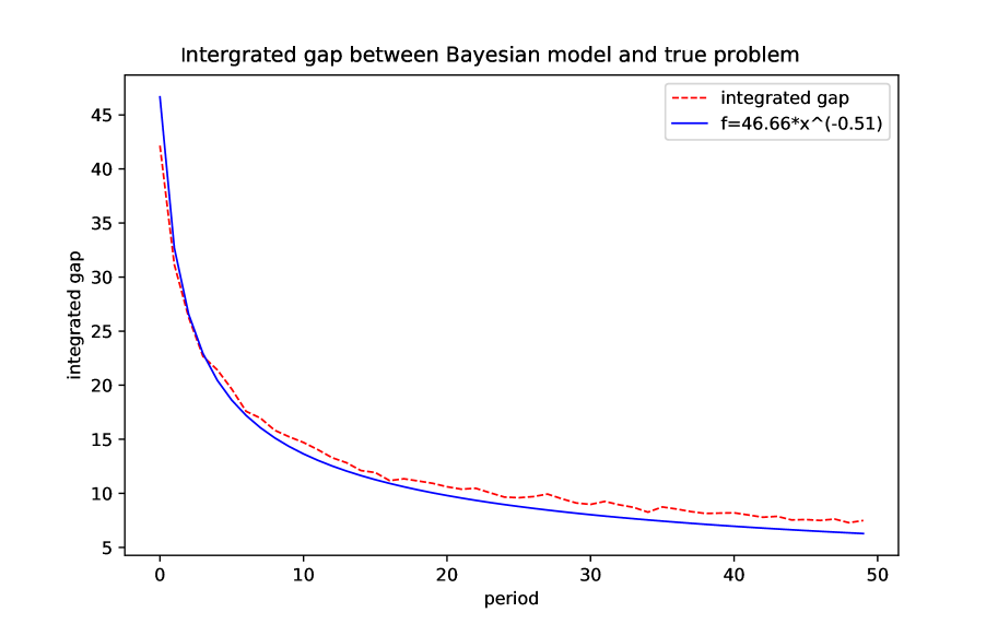
To make the Bayesian updating in closed form, we choose a Gamma prior $\Gamma(\alpha_{0},\beta_{0})$ with $\alpha_{0}=\beta_{0}=1$ on the unknown parameter $\frac{1}{\theta}$. Given $n$ observed data $\xi_{1},\ldots,\xi_{n}$, the posterior is also a Gamma distribution with parameter $\alpha^{\prime}=\alpha_{0}+n$, $\beta^{\prime}=\beta_{0}+\sum_{i=1}^{n}\xi_{i}$. In episode $N$, we update the Bayesian posterior with the observed data and then solve the above inventory control problem with probability distribution $P_{*}$ in (5.14) replaced by posterior probability distribution $P_{N}$ for the episodic value function $V_{N}$. We use a large number ($10^{5}$) of samples from $P_{*}$ or $P_{N}$ to approximate the expectation in (5.14) to obtain the true optimal value function $V^{*}$ or the episodic optimal value function $V_{N}$. We then plot the integrated gap between $V_{N}$ and $V^{*}$ with the gap computed as $\int_{\mathcal{X}}|V_{N}(x)-V^{*}(x)|d\mu^{*}(x)$, where $\mu^{*}$ is the stationary distribution (or occupancy measure of states) under true optimal policy $\pi^{*}$ of the original problem.

Figure 1: Convergence rate of episodic value functions

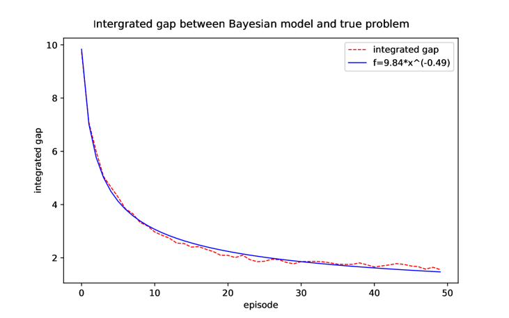
Figure 1 shows integrated gap between $V_{N}$ and $V^{*}$ in terms of episodes. The result is computed by running 200 replications. In each episode, new data of batch size $20$ is used to update the Bayesian posterior. To see how fast it converges to 0, we fit a regression model $f(x)=a*x^{b}$ with optimal values $a=9.84$ and $b=-0.49$, which is shown as the blue curve in the figure. The close value of $b$ to $-0.5$ verifies the theoretical result of convergence rate $O(N^{-1/2})$ with $N$ being the number of episodes.

(a) Empirical pdf

(b) Normal QQ plot

Figure 2: Asymptotic normality of episodic value functions

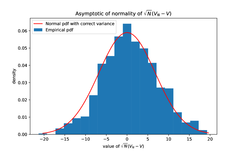
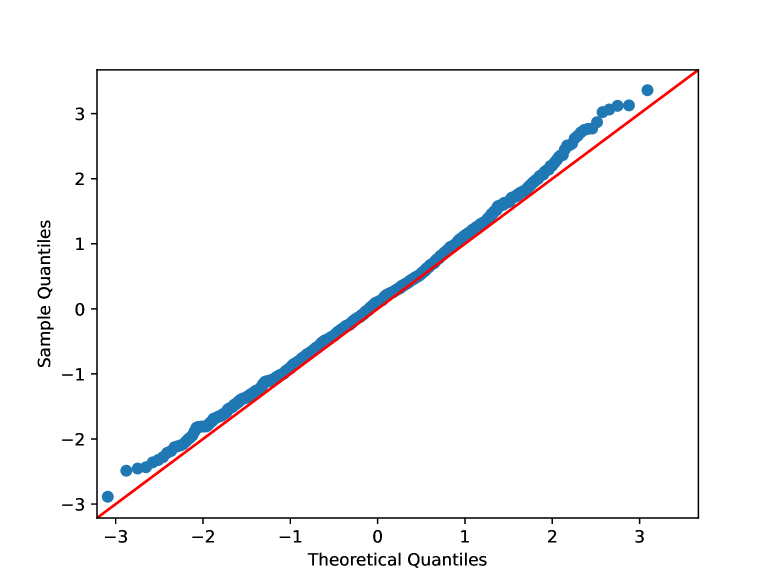
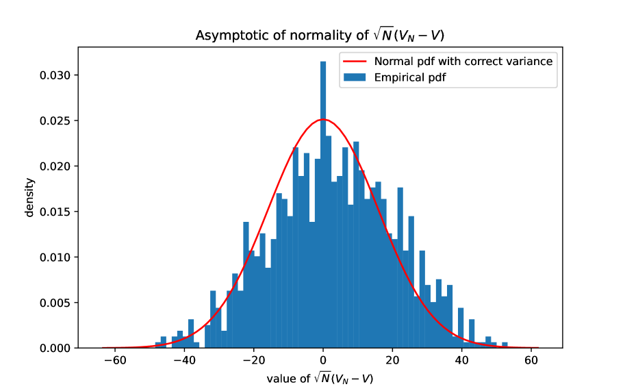
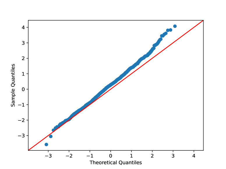
In Figure 2, we test the asymptotic normality of $\sqrt{N}(V_{N}-V^{*})$. For this specific test, we set the mean of demand $\theta=1$ to reduce the Monte Carlo estimation error of $V_{N}$ in the experiment. Other parameters are the same as in Figure 1. In Figure 2(a), the blue bar chart represents the empirical density of $\sqrt{N}(V_{N}-V)$ at $x_{0}=0$ and $N=100$, with $1000$ replications. The red curve represents the theoretical normal pdf with mean $0$ and standard deviation $\sigma^{c}$ computed according to (3.26). Figure 2(b) is the QQ plot, which plots the quantile of the empirical distribution $\frac{\sqrt{N}(V_{N}-V^{*})}{\sigma^{c}}$ (empirical quantile) against the quantile of the standard normal distribution (theoretical quantile). As both figures indicate, the empirical pdf coincides with the theoretical pdf well, verifying the asymptotic normality result in Section 3.2.

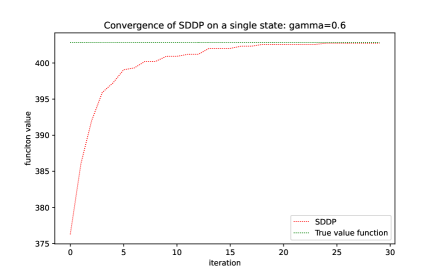
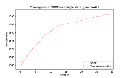
Next, we demonstrate the performance of Algorithm 2 on this problem. We run two different versions of this algorithm, both of which use SDDP to solve episode-wise Bayesian problem but differs in whether warm starting with the lower approximation from the previous episode. Both versions use the sample size $M=100$. In Figure 3, we plot the convergence of the SDDP algorithm on the final episode out of 5 episodes in total. The x-axis is the number of SDDP iteration number, and the y-axis is the function value (episodic value function $V_{N}$, and the approximate value function $\underline{{\cal V}}_{N}$ generated by Algorithm 2) evaluated at the initial point $x_{0}=1$. We vary the discount factor from 0.6 (left plot) to 0.9 (right plot).

Figure 3: SDDP algorithm with single episode for 1-D inventory control.

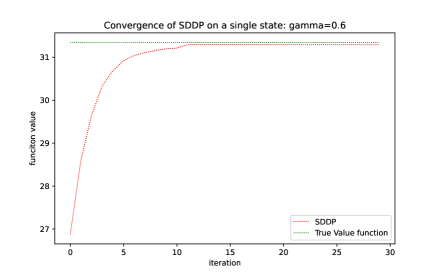
Figure 3 indicates the SDDP converges to the true value by maintaining an increasing lower approximation. It takes about 5 iterations to converge for $\gamma=0.6$ and takes about 30 iterations to converge for $\gamma=0.9$. The convergence is fast, considering the control and state space are both continuous.

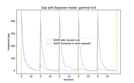
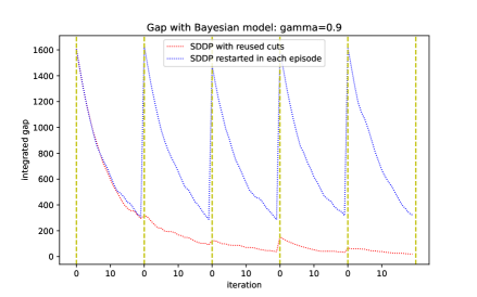
Figure 4 plots the integrated gap between $\underline{{\cal V}_{N}}$ and $V_{N}$ over the stationary distribution $\mu_{N}$ under the episodic optimal policy $\pi_{N}$, i.e., $\int_{\mathcal{X}}(V_{N}(x)-\underline{{\cal V}}_{N}(x))d\mu_{N}(x)$, where we drop the absolute value since $\underline{{\cal V}}_{N}$ is always a lower bound of $V_{N}$. The vertical dashed line shows the switch between two successive episodes. The left and right plots vary in the discount factor $\gamma$.

Figure 4: SDDP algorithm for 1-D Inventory Control.

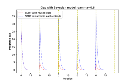
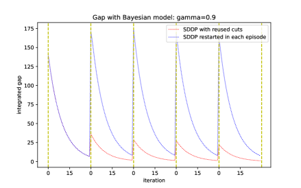
Figure 4 shows that within each episode SDDP converges to the optimal value ${\cal V}_{N}$ efficiently. By comparing the algorithm with warm start (red curve) and without warm start (blue curve), we can see the benefits of reusing the previous lower approximation in the next episode. Without warm start, the lower approximation of each episode starts from a large value (about $35$ for $\gamma=0.6$ and $150$ for $\gamma=0.9$) since we initialize $\underline{{\cal V}}_{N}$ by using a loose lower bound. When reusing the previous lower approximation, the initial gap starts from a relatively small value (lower than $5$ for $\gamma=0.6$ and $30$ for $\gamma=0.9$). This is even more beneficial in the later episode as the Bayesian posterior concentrate more on the true value, and as a result, more than $50\%$ of cuts of the previous episode remain valid for the new episode.

Figure 5: Convergence rate of episodic value functions

(a) Empirical pdf

(b) Normal QQ plot

Figure 6: Asymptotic normality of episodic value functions

Figure 7: SDDP algorithm with single episode for 5-D Inventory Control.

Figure 8: SDDP algorithm for the 5-D Inventory Control.

5.2 5-D Inventory Control

We also test on the multi-dimensional version of this inventory example. Suppose we have $N\_prod=5$ types of products. The $i$th product has the order cost $c_{i}=1+0.5*\sin{(i-1)}$, holding cost $h_{i}=2+0.5*\sin{(i-1)}$ and backorder penalty cost $b_{i}=3+0.5*\sin(i-1)$, for $i=1,2,\ldots,5$. The state is a five-dimensional vector, with each component being the current inventory level of each product. Assume the demand for each product follows an exponential distribution with unknown mean $\theta_{i}=10+0.5i,i=1,2,\ldots,5$.

We first show the convergence rate and asymptotic normality of the episodic value functions to the true optimal value function, and then demonstrate Algorithm 2 with or without reusing past lower approximation. Similar as for the 1-D case, due to the larger estimation error of ${\cal V}_{N}$, in Figure 6 we set the mean of demand distribution for the $i$th product to be $1+\sin(i-1)*0.2$ and still use $10^{5}$ samples from $P_{*}$ or $P_{N}$ to approximate the expectation in $V^{*}$ and $V_{N}$. We evaluate $V_{N}$ with $50$ episodes for testing convergence in Figure 5. In Figure 6, for testing asymptotic normality we evaluate $V_{N}$ at $N=100$ and at state $x_{0}=\mathbf{0}$. The empirical pdf and QQ plot are calculated with 1000 replications. In Figure 7 and 8, we use sample size $M=100$ in Algorithm 2 and run for 5 episodes with number of SDDP iterations $K=30$ for each episode. In Figure 7, the lower approximation is evaluated at state $x_{0}=\mathbf{0}$.

Similar results hold as in 1-D case in Figures 5, 6, 7 and 8. It is worth noting that there are more benefits of reusing past lower approximation in the higher-dimensional problem, in particular, because SDDP converges slower in high dimensions. For example, in the second plots of Figures 7 and 8 with discount factor $\gamma=0.9$, the difference between the two algorithms (with and without warm start) is starker, and we note that with warm start the percentage of reused previous cuts is higher than $80\%$ in the last three episodes.

6 Conclusions and Future Research

In this paper, we propose an episodic Bayesian approach to address unknown randomness distribution in stochastic optimal control. It incorporates Bayesian learning of the unknown distribution with optimization of the control policy. In each episode, the current policy is exercised and more data on the randomness are collected to update the Bayesian posterior, which is in turn used to update the control policy in the next episode. We show that the episodic value functions converge almost surely to the true optimal value function at an asymptotic rate of $1/\sqrt{N}$, where $N$ is the number of data points (which is also the number of episodes when the episode length is $1$). For problems where value functions are convex, we develop a computational algorithm based on the stochastic dual dynamic programming approach, with a warm start for each episode by reusing the value function approximation from the previous episode. Our numerical results on an inventory control problem verify the theoretical results and also demonstrate the effectiveness of the proposed algorithm.

There are several directions for future research. First, we have assumed that the length of each episode is constant, but it could be time-varying or even random in accordance with the Bayesian learning of the unknown distribution. For example, the episode length could become longer as the Bayesian posterior stabilizes at later times. We have also assumed the Bayesian average problem is solved to optimality in each episode, but it is not always possible or necessary to do so. There should be a balance between the estimation error (due to Bayesian learning from finite data) and optimization error (due to sub-optimality of the solution to the episodic Bayesian average problem). Second, as we mentioned in the paper, the assumed parametric form for the unknown randomness distribution could lead to model misspecification, and therefore, the Bayesian distributionally robust optimization approach for static (one-stage) optimization problems [16] could be a valuable direction to investigate for the dynamic problem here.

7 Appendix

Suppose now that the control set depends on the state vector and is given in the form

$${\cal U}(x):=\{u\in{\cal U}:g_{k}(x,u)\leq 0,\;k=1,...,K\}.$$ (7.1)

The counterpart of the Bellman equation (2.8) is

$$V(x)=\inf\left\{{\mathbb{E}}\left[c(x,u,\xi)+\gamma V\big{(}F(x,u,\xi)\big{)}\right]:u\in{\cal U},\;g(x,u)\leq 0\right\},$$ (7.2)

where $g(x,u)=(g_{1}(x,u),...,g_{K}(x,u))$. The counterparts of the value functions $V^{*}$ and $V^{*}_{N}$ are given as solutions of the Bellman equation of the form (7.2) when the expectation is taken with respect to the corresponding distributions $f(\cdot|\theta^{*})$ and $P_{N}$. The value functions are convex if in addition to Assumption 4.1 the functions $g_{k}(x,u)$, $i=1,...,K$, are convex in $(x,u)$.

For a current approximation $\underline{{\cal V}}_{N}$ of the value function the required subgradient at a trial point $\bar{x}$ is given by an optimal solution of the dual of the problem

$$\begin{array}[]{cll}\min\limits_{u\in{\cal U},\,z\in{\mathbb{R}}^{M}}&\sum_{j=1}^{M}c_{j}(\bar{x},u)+z_{j}\\ {\rm s.t.}&\underline{{\cal V}}_{N}(A_{j}\bar{x}+B_{j}u+b_{j})\leq z_{j},\;j=1,...,M,\\ &g_{k}(\bar{x},u)\leq 0,\;k=1,...,K.\end{array}$$ (7.3)

If the set ${\cal U}$ is polyhedral and the functions $\underline{{\cal V}}_{N}(\cdot)$, $c_{j}(\cdot,\cdot)$, $j=1,...,M$, and $g_{k}(\cdot,\cdot)$, $k=1,...,K$, are given as maxima of the respective (finite) sets of affine functions, problem (7.3) can be formulated as a linear programming problem.

References

- [1] T. Basar and P. Bernhard. -optimal control and related minimax design problems – A dynamic game approach. Birkhauser Boston, 2008.
- [2] D.P. Bertsekas and S.E. Shreve. Stochastic Optimal Control, The Discrete Time Case. Academic Press, New York, 1978.
- [3] Tomasz R. Bielecki, Tao Chen, Igor Cialenco, Areski Cousin, and Monique Jeanblanc. Adaptive robust control under model uncertainty. SIAM Journal on Control and Optimization, 57(2):925–946, 2019.
- [4] Joseph L. Doob. Application of the theory of martingales. Actes du Colloque International Le Calcul des Probabilites et ses applications, pages 23–27, 1948.
- [5] Michael O’Gordon Duff. Optimal Learning: Computational procedures for Bayes-adaptive Markov decision processes. University of Massachusetts Amherst, 2002.
- [6] Itzhak Gilboa and David Schmeidler. Maxmin expected utility with non-unique prior. Journal of Mathematical Economics, 18:141–153, 1989.
- [7] J. I. González-Trejo, O. Hernández-Lerma, and L. F. Hoyos-Reyes. Minimax control of discrete-time stochastic systems. SIAM Journal on Control and Optimization, 41(5):1626–1659, 2002.
- [8] L. P. Hansen, G. Sargent, G. Turmuhambetova, and N. Williams. Robust control and model misspecification. J. Econom. Theory, 2006.
- [9] P. R. Kumar and P. Varaiya. Stochastic Systems: Estimation, Identification, and Adaptive Control, chapter Chapter 11: Bayesian Adaptive Control. Prentice Hall, 2015.
- [10] A. E. B. Lim, G. J. Shanthikumar, and Z. J. Max Shen. Model uncertainty, robust optimization and learning. Tutorials in Operations Research, INFORMS, pages 66–94, 2006.
- [11] Yifan Lin, Yuxuan Ren, and Enlu Zhou. Bayesian risk Markov decision processes. In S. Koyejo, S. Mohamed, A. Agarwal, D. Belgrave, K. Cho, and A. Oh, editors, Advances in Neural Information Processing Systems, volume 35, pages 17430–17442, 2022.
- [12] U. Rieder. Bayesian dynamic programming. Adv. Appl. Prob., pages 330–348, 1975.
- [13] Lorraine Schwartz. On Bayes procedures. Zeitschrift für Wahrscheinlichkeitstheorie und Verwandte Gebiete, 4:10–26, 1965.
- [14] A. Shapiro and Y. Cheng. Central limit theorem and sample complexity of stationary stochastic programs. Operations Research Letters, 49:676–681, 2021.
- [15] A. Shapiro, D. Dentcheva, and A. Ruszczyński. Lectures on Stochastic Programming: Modeling and Theory. SIAM, Philadelphia, third edition, 2021.
- [16] Alexander Shapiro, Enlu Zhou, and Yifan Lin. Bayesian distributionally robust optimization. SIAM Journal on Optimization, 33(2):1279–1304, 2023.
- [17] Mihai Sîrbu. A note on the strong formulation of stochastic control problems with model uncertainty. Electronic Communications in Probability, 19:1–10, 2014.
- [18] I. Tzortzis, C. D. Charalambous, and T. Charalambous. Infinite horizon average cost dynamic programming subject to total variation distance ambiguity. SIAM Journal of Control and Optimization, 57(4):2843–2872, 2019.
- [19] A.W. van der Vaart. Asymptotic Statistics. Cambridge Univ. Press, 1998.
- [20] Bart P. G. Van Parys, Daniel Kuhn, Paul J. Goulart, and Manfred Morari. Distributionally robust control of constrained stochastic systems. IEEE Transactions on Automatic Control, 61(2):430–442, 2016.
- [21] Insoon Yang. Wasserstein distributionally robust stochastic control: A data-driven approach. IEEE Transactions on Automatic Control, 66:3863–3870, 2018.
- [22] P.H. Zipkin. Foundation of inventory management. McGraw-Hill, 2000.