Certifying Stability and Performance of Uncertain Differential-Algebraic Systems: A Dissipativity Framework

Abstract

This paper presents a novel framework for characterizing dissipativity of uncertain dynamical systems subject to algebraic constraints. The main results provide sufficient conditions for dissipativity when uncertainties are characterized by integral quadratic constraints. For polynomial or linear dynamics, these conditions can be efficiently verified through sum-of-squares or semidefinite programming. The practical impact of this work is illustrated through a case study that examines performance of the IEEE 39-bus power network with uncertainties used to model a set of potential line failures.

1 Introduction

Dissipativity theory [1] relates input-output properties of dynamical systems to the dissipation of so-called storage functions over trajectories [2]. Storage functions generalize Lyapunov functions for closed systems to open systems with inputs and outputs: rather than decreasing along trajectories, the time derivative of the storage function along trajectories is upper bounded by a supply rate that describes a relation of the system’s inputs and outputs. Appropriate choices of supply rate lead to special cases of dissipativity, such as passivity, stability and $L_{2}$ gain bounds. Moreover, a dissipativity framework allows for incorporation of uncertainties described by integral quadratic constraints [3, 4].

Classical dissipativity applies to system dynamics described by ordinary differential equations (ODEs). Here, we develop a dissipativity framework that applies to uncertain systems described by differential-algebraic equations (DAEs). This framework unifies the study of key system properties, ranging from stability to performance, while accommodating classes of model uncertainty described by integral quadratic constraints and obviating the need to eliminate algebraic equations. DAEs can model dynamical systems with constraints and arise in chemical, electrical, and mechanical engineering applications [5], e.g., electric circuit models constrained to conserve charge, fluid flow modeled by the Navier-Stokes equations subject to an incompressibility constraints, or mechanical system motion subject to holonomic constraints [6].

Many classical results have been extended from the ODE to the DAE setting, including controllability and observability [7], and controller [8] and observer [9] design for linear systems. Specific subclasses of dissipativity that have been examined for DAEs include positive realness of linear DAE systems [10] and Lyapunov stability and passivity of nonlinear DAE systems [11]. However, incorporation of uncertainties into dissipativity analysis of DAE systems is less prevalent; one exception is [12] which analyzes stability of linear DAE systems subject to polytopic uncertainties. Despite the vast literature on disspativity and on DAEs, a general dissipativity framework for uncertain and nonlinear differential-algebraic systems is lacking.

In this manuscript, we extend the notion of dissipativity to linear and nonlinear DAE systems with uncertainties and provide sufficient conditions for dissipativity when the uncertainty is described by quadratic constraints. For linear or polynomial dynamics, we show that these conditions can be verified numerically with linear matrix inequalities or Sum-of-Squares programming, respectively.

This work is motivated by DAE models with algebraic constraints arising from network interconnections, e.g., dynamics of multibody systems with interconnection constraints [13], power networks with algebraic power flow constraints [14], and implicit neural networks with outputs defined as the solutions to fixed-point equations [15]. When the algebraic constraint is invertible, the DAE system may be equivalently represented as a standard ODE, e.g., power network DAEs can be converted to an ODE through a Kron reduction procedure [16]. However, this suffers a loss of the network structure that is captured in the algebraic constraint; this is illustrated in a case study of a power network with with uncertain line failure presented in Section 5.

The remainder of the paper is structured as follows. In Section 2, a DAE model and an IQC characterization of uncertainties are presented; the notion of dissipativity for this model is formalized. Section 3 derives a sufficient condition for dissipativity of an uncertain DAE system. This condition is shown to be confirmable numerically in Section 3.2 for polynomial dynamics and Section 4 for the linear setting. A power network with an uncertain line failure is analyzed as a case study in Section 5.

2 Problem Set-Up: Uncertain Differential-Algebraic Systems

We consider a system with time-invariant state dynamics, subject to algebraic constraints:

$$\dot{\boldsymbol{x}}(t) =f(\boldsymbol{x}(t),\boldsymbol{v}(t),\boldsymbol{w}(t),\boldsymbol{\xi}(t))$$ (1a)

$$0 =g(\boldsymbol{x}(t),\boldsymbol{v}(t),\boldsymbol{w}(t),\boldsymbol{\xi}(t))$$ (1b)

$$\boldsymbol{y}(t) =h(\boldsymbol{x}(t),\boldsymbol{v}(t)),$$ (1c)

where $\boldsymbol{x}(t)\in\mathbb{R}^{n}$ is the state, $\boldsymbol{v}(t)\in\mathbb{R}^{m}$ is the algebraic variable, $\boldsymbol{w}(t)\in\mathbb{R}^{p}$ is an exogenous disturbance, and $\boldsymbol{y}(t)\in\mathbb{R}^{q}$ is an output. $\boldsymbol{\xi}(t)\in\mathbb{R}^{\ell}$ captures additional dynamics, e.g., uncertainties, and is modeled as the output of a bounded, causal system $\Delta:L_{2}^{n}\times L_{2}^{m}\rightarrow L_{2}^{\ell}$:

$$\boldsymbol{\xi}=\Delta\left(\boldsymbol{x},\boldsymbol{v}\right).$$ (2)

Bold letters denote signals, ${\boldsymbol{x}}:[0,\tau]\rightarrow\mathbb{R}^{n}$, and non-bold letters denote points, $x\in\mathbb{R}^{n}$. We assume an equilibrium point exists and is shifted to $x=0$; i.e., $f(0,v_{0},0,0)=0,g(0,v_{0},0,0)=0$ for some $v_{0}.$ For $\boldsymbol{\xi}=0$, (1) is a differential-algebraic equation (DAE) in semi-explicit form [6, 5].

Assumption 1

The initial conditions of (1) are consistent, e.g., they satisfy the constraints (1b). Inputs to the system are sufficiently smooth. Given consistent initial conditions and sufficiently smooth inputs, a unique solution $\boldsymbol{x},\boldsymbol{v},\boldsymbol{\xi},\boldsymbol{y}$, exists for the system (1)-(2) over an interval of time $t\in[0,\tau]$.

Methods for determining admissible initial conditions can be found in, e.g., [17], and existence and uniqueness of solutions can be confirmed through, e.g., geometric approaches [18], [19], theory of differential equations on manifolds [20], or computational methods [21]. Further details on the solvability of DAEs are beyond the scope of this work; we refer the reader to [6, 5] and the references therein for a more comprehensive study.

2.1 Dissipativity of DAE Systems

We begin by formalizing the notion of dissipativity for uncertain DAE systems.

Definition 1

Under Assumption 1, the DAE system (1)-(2) is dissipative with respect to the supply rate $s(\cdot,\cdot)$ if there exists a positive definite function $V(\cdot)$, called a storage function, such that $V(0)=0$ and

$$V(\boldsymbol{x}(T))-V(\boldsymbol{x}(0))\leq\int_{0}^{T}s(\boldsymbol{w}(t),h(\boldsymbol{x}(t),\boldsymbol{v}(t)))dt$$ (3)

for all $T\in[0,\tau].$

Note that $\boldsymbol{x},\boldsymbol{w},\boldsymbol{v},$ and $\boldsymbol{\xi}$ in (3) satisfy

$$0=g(\boldsymbol{x}(t),\boldsymbol{v}(t),\boldsymbol{w}(t),\boldsymbol{\xi}(t))$$ (4)

due to constraint (1b) of the system dynamics. Supply rates of interest include:

• $s(w,y)=w^{\top}y$ corresponding to passivity,

• $s(w,y)=w^{\top}w-\gamma^{2}y^{\top}y$ corresponding to an $L_{2}$ gain bound of $\gamma$,

• $s(w,y)\equiv 0$ corresponding to stability of the origin; in this case the storage function $V(\cdot)$ serves as a Lyapunov function.

This definition is difficult to verify in the presence of unknown $\Delta$. In what follows we derive sufficient conditions for dissipavity when $\Delta$ is unknown, but satisfies known quadratic constraints.

2.2 Integral Quadratic Constraints

Figure 1: Block diagram representation of uncertain system $\Delta$ and virtual filter $\Psi$. $\Psi$ is utilized to provide a more general input-output characterization of $\Delta$ via the integral quadratic constraint $\int_{0}^{\infty}z(t)^{\top}Mz(t)dt\leq 0$ for some $M=M^{\top},$ where $z$ is the output of $\Psi$.

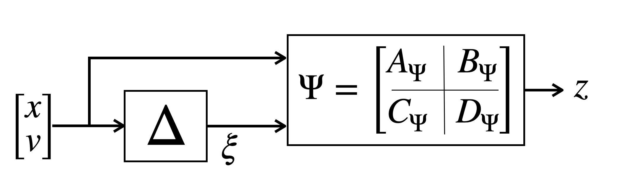
We characterize $\Delta$ in (2) through input-output properties with the framework of integral quadratic constraints (IQCs) [4, 22]. As depicted in Figure 1, the input signals $\boldsymbol{x},\boldsymbol{v}$ and output signal $\boldsymbol{\xi}$ of $\Delta$ are passed through a “virtual filter” $\Psi$ defined by the stable linear dynamics:

$$\dot{\boldsymbol{\psi}}(t) =A_{\Psi}\boldsymbol{\psi}(t)+B_{\psi}{\small{\left[\begin{array}[]{c}\boldsymbol{x}(t)\\ \boldsymbol{v}(t)\\ \boldsymbol{\xi}(t)\end{array}\right]}},~{}~{}\boldsymbol{\psi}(0)=0$$ (5)

$$\boldsymbol{z}(t) =C_{\Psi}\boldsymbol{\psi}(t)+D_{\Psi}{\small{\left[\begin{array}[]{c}\boldsymbol{x}(t)\\ \boldsymbol{v}(t)\\ \boldsymbol{\xi}(t)\end{array}\right]}}.$$

For $M=M^{\top}$, $\Delta$ satisfies the hard IQC defined by $(\Psi,M)$ if

$$\int_{0}^{T}\boldsymbol{z}(t)^{T}M\boldsymbol{z}(t)dt\leq 0$$ (6)

for all $T\geq 0$. This is clearly satisfied if

$$\boldsymbol{z}(t)^{\top}M\boldsymbol{z}(t)\leq 0,~{}~{}\forall t\geq 0,$$ (7)

and we say $\Delta$ satisfies the pointwise quadratic constraint defined by $(\Psi,M)$. In the simple case that $\Psi$ is the identity operator, (6) reduces to

$$\int_{0}^{T}{\small{\left[\begin{array}[]{c}\boldsymbol{x}(t)\\ \boldsymbol{v}(t)\\ \boldsymbol{\xi}(t)\end{array}\right]}}^{\top}M{\small{\left[\begin{array}[]{c}\boldsymbol{x}(t)\\ \boldsymbol{v}(t)\\ \boldsymbol{\xi}(t)\end{array}\right]}}dt\leq 0.$$ (8)

3 Conditions for Dissipativity of Differential-Algebraic Systems

This section presents a sufficient condition for dissipativity of DAE systems with uncertainties described by IQCs and shows this can be confirmed numerically for polynomial DAEs.

Theorem 1

Consider the DAE system (1)-(2) and assume $\Delta$ satisfies the IQC defined by $(\Psi,M)$. This system is dissipative w.r.t. the supply rate $s(\cdot,\cdot)$ if there exist $\tau,\lambda\geq 0$, a matrix $P_{\Delta}\succeq 0$, and a positive definite $V(\cdot)$ satisfying $V(0)=0$ and

$$\triangledown V(x)^{\top}f(x,v,w,\xi)+{\psi}^{\top}P_{\Delta}\Big{(}A_{\psi}^{\top}\psi\small{+}B_{\psi}\left[\begin{array}[]{c}x\\ {v}\\ {\xi}\end{array}\right]\Big{)}$$ (9)

$$+\Big{(}A_{\psi}^{\top}\psi\small{+}B_{\psi}\left[\begin{array}[]{c}x\\ {v}\\ {\xi}\end{array}\right]\Big{)}^{\top}P_{\Delta}\psi$$

$$\leq~{}s\big{(}w,h(x,v)\big{)}+\lambda g(x,v,w,\xi)^{\top}g(x,v,w,\xi)~{}+$$

$$\tau\Big{(}C_{\psi}\psi+D_{\psi}{\small{\left[\begin{array}[]{c}x\\ v\\ \xi\end{array}\right]}}\Big{)}^{\top}M\Big{(}C_{\psi}\psi+D_{\psi}{\small{\left[\begin{array}[]{c}x\\ v\\ \xi\end{array}\right]}}\Big{)},$$

for all $\psi,x,v,\xi,w.$

Proof of Theorem 1: Integrating (LABEL:eq:nonlinear_general_int) from $t=0$ to $T$ along trajectories of (1) and (5) and using the filter initial condition $\boldsymbol{\psi}(0)=0$ gives

$$V(\boldsymbol{x}(T))+\boldsymbol{\psi}(T)^{T}P_{\Delta}{\boldsymbol{\psi}}(t)-V(\boldsymbol{x}(0))$$ (10)

$$\leq\int_{0}^{T}s\big{(}\boldsymbol{w}(t),h\big{(}\boldsymbol{x}(t),\boldsymbol{v}(t)\big{)}\big{)}dt~{}+$$

$$~{}~{}\lambda\underbrace{\int_{0}^{T}(\star)^{\top}g(\boldsymbol{x}(t),\boldsymbol{v}(t),\boldsymbol{w}(t),\boldsymbol{\xi}(t))dt}_{(I)}+$$

$$~{}~{}\tau\underbrace{\int_{0}^{T}(\star)^{\top}M\Big{(}C_{\psi}\boldsymbol{\psi}(t)+D_{\psi}{\small{\left[\begin{array}[]{c}\boldsymbol{x}(t)\\ \boldsymbol{v}(t)\\ \boldsymbol{\xi}(t)\end{array}\right]}}\Big{)}dt,}_{(II)}$$

where the terms denoted by $(\star)$ can each be inferred by symmetry. By the classical s-procedure, the existence of $\tau,\lambda\geq 0$ satisfying (LABEL:eq:pf1) ensures that nonpositivity of terms $(I)$ and $(II)$ imply

$$V(\boldsymbol{x}(T))-V(\boldsymbol{x}(0))+\boldsymbol{\psi}(T)^{T}P_{\Delta}{\boldsymbol{\psi}}(T)~{}\leq$$ (11)

$$\int_{0}^{T}s\big{(}\boldsymbol{w}(t),h\big{(}\boldsymbol{x}(t),\boldsymbol{v}(t)\big{)}\big{)}dt.$$

Nonposivity of $(I)$ and $(II)$ follow from (4) and that $\Delta$ satisfies the IQC defined by $(\Psi,M)$, respectively. (3) follows from (LABEL:eq:1) since $P_{\Delta}\succeq 0$. $\blacksquare$

Remark 1

We can view

$$\tilde{V}(x,\psi):=V(x)+\psi^{\top}P_{\Delta}\psi$$ (12)

as a storage function of the augmented system of DAE (1) and filter (5). $P_{\Delta}=0$ amounts to searching for a storage function of DAE (1) alone; Searching for a combined storage function (nonzero $P_{\Delta}$) introduces another term to the left hand side of (LABEL:eq:nonlinear_general_int) whose negativity may help this inequality hold. Without uncertainty or with uncertainty characterized by a pointwise constraint, we may assume $P_{\Delta}=0.$

3.1 Dissipativity of Systems without Uncertainty

Theorem 1 simplifies in the case of no uncertainty, as stated in the following corollary.

Corollary 1

The DAE system (1), with $\boldsymbol{\xi}=0$, is dissipative w.r.t. the storage function $s(\cdot,\cdot)$ if there exists $\lambda\geq 0$ and a positive definite $V(\cdot)$ such that $V(0)=0$ and

$$\triangledown V(x)^{\top}f(x,v,w,0)\leq$$ (13)

$$s\big{(}w,h(x,v)\big{)}+\lambda g(x,v,w,0)^{\top}g(x,v,w,0)$$

for all points $x,v,w$.

3.2 Numerical Solutions for Polynomial Dynamics

When the DAE system is described by polynomials, the storage function (12) can be found numerically with a sum-of-squares approach.

A polynomial $p$ is sum-of-squares (SOS) if there exist polynomials $p_{1},\dots,p_{n}$ such that $p=\sum_{i=1}^{n}p_{i}^{2}$. A polynomial being SOS implies it is nonnegative. Let $\Sigma[x]$ be the set of SOS polynomials in $x$, and $\Sigma[(x,v,w,\xi,\psi)]$ be the set of SOS polynomials in $x,v,w,\xi$ and $\psi$. Then, for polynomial $f,g,$ and $h$ and a polynomial supply rate $s$, we can verify dissipativity through Theorem 1 by finding nonnegative scalars $\tau$ and $\lambda$, a positive definite matrix $P_{\Delta}$, and a $V\in\Sigma[x]$ such that $V(x)-\epsilon x^{\top}x\in\Sigma[x]$ and

$$s(w,h(x,v))+\lambda\cdot(\star)^{\top}g(x,v,w,\xi)$$ (14)

$$+\tau\cdot(\star)^{\top}M\Big{(}C_{\psi}\psi+D_{\psi}{\small{\left[\begin{array}[]{c}x\\ v\\ \xi\end{array}\right]}}\Big{)}$$

$$-\triangledown V(x)^{\top}f(x,v,w,\xi)-\psi^{\top}P_{\Delta}\psi$$

$$-\psi^{\top}P_{\Delta}\Big{(}A_{\psi}\psi+B_{\psi}{\small{\left[\begin{array}[]{c}x\\ v\\ \xi\end{array}\right]}}\Big{)}$$

$$\in\Sigma[(x,v,w,\xi,\psi)]$$

where $\epsilon$ is small and positive and each of the terms $(\star)$ can be inferred by symmetry.

Example 1

Consider the polynomial DAE system:

$$\dot{\boldsymbol{x}}_{1}(t) =-\boldsymbol{x}_{1}(t)+\boldsymbol{v}(t)$$ (15)

$$\dot{\boldsymbol{x}}_{2}(t) =-\boldsymbol{x}_{1}(t)-\boldsymbol{x}_{2}(t)$$

$$0 =\boldsymbol{x}_{1}(t)^{2}+\left(\boldsymbol{x}_{2}(t)^{2}+5\right)\boldsymbol{v}(t).$$

Applying (14) to this system to show stability of the origin gives the following equations

$$V(x)-\epsilon x^{\top}x \in\Sigma[x],$$

$$\lambda g(x,v)^{\top}g(x,v)-\triangledown V(x)^{\top}f(x,v) \in\Sigma[(x,v)].$$

To implement this, we use the SOSTOOLS MATLAB toolbox [23] and the SeDuMi solver [24]. We allow $V$ to be a polynomial of degree $\leq 4$. For $\epsilon=10^{-3}$, SeDuMi finds a solution $\lambda=0.59504$ and $V(x)=0.00017634x_{1}^{4}+0.0012261x_{1}^{2}x_{2}^{2}+0.0027498x_{1}x_{2}^{3}+0.0023039x_{2}^{4}+0.013246x_{1}^{3}-0.013733x_{1}^{2}x_{2}-0.055089x_{1}x_{2}^{2}-0.056305x_{2}^{3}+0.40316x_{1}^{2}+0.67688x_{1}x_{2}+0.57717x_{2}^{2}$.

4 Dissipativity of Linear Differential-Algebraic Systems

For linear DAE dynamics, dissipativity can be verified with feasibility of an LMI. The linear DAE model is:

$$\dot{\boldsymbol{x}}(t){\small{=}}A\boldsymbol{x}(t){\small{+}}B_{v}\boldsymbol{v}(t)+B_{w}\boldsymbol{w}(t)+B_{\xi}\boldsymbol{\xi}(t)$$ (16a)

$$0{=}F\boldsymbol{x}(t)+G_{v}\boldsymbol{v}(t)+G_{w}\boldsymbol{w}(t)+G_{\xi}\boldsymbol{\xi}(t)$$ (16b)

$$\boldsymbol{y}(t)=C\boldsymbol{x}(t)+D_{v}\boldsymbol{v}(t),$$ (16c)

where

$$\boldsymbol{\xi}=\Delta(\boldsymbol{x},\boldsymbol{v})$$ (17)

can describe nonlinearites such as model uncertainties [25] or saturations [26]. We restrict our attention to quadratic supply rates:

$$s(w,y)=\left[\begin{array}[]{c}y\\ w\end{array}\right]^{\top}\tilde{X}_{s}\left[\begin{array}[]{c}y\\ w\end{array}\right]\\$$

which, using the equality $y=Cx+D_{v}v$, can be written as

$$s(w,Cx\small{+}D_{v}v){\small{=}}\left[\begin{array}[]{c}x\\ w\end{array}\right]^{\top}\left[\begin{array}[]{cc}X_{xx}&X_{xw}\\ X_{xw}^{\top}&X_{ww}\end{array}\right]\left[\begin{array}[]{c}x\\ w\end{array}\right]$$ (18)

For linear dynamics and quadratic supply rates, there is no loss [1] in restricting a storage function $V(\cdot)$ to be quadratic:

$$V(x)=x^{\top}Px,~{}~{}P=P^{\top}\succ 0.$$ (19)

4.1 Linear DAE without Uncertainty

In the case of $\boldsymbol{\xi}=0$, feasibility of an LMI is both necessary and sufficient for dissipativity, as stated next. The proof of this result is in Appendix A.

Proposition 1

The linear DAE system (16), with $\boldsymbol{\xi}=0$, is dissipative w.r.t. the quadratic supply rate (18) if and only if there exists $\lambda\geq 0$ and a matrix $P\succ 0$ such that

$$\left[\begin{array}[]{ccc}A^{\top}P+PA&PB_{v}&PB_{w}\\ B_{v}^{\top}P&0&0\\ B_{w}^{\top}P&0&0\end{array}\right]\preceq$$ (20)

$$\left[\begin{array}[]{ccc}X_{xx}&0&X_{xw}\\ 0&0&0\\ X_{xw}^{\top}&0&X_{ww}\end{array}\right]{\small{+}}\lambda\left[\begin{array}[]{c}F^{\top}\\ G_{v}^{\top}\\ G_{w}^{\top}\end{array}\right]\left[\begin{array}[]{ccc}F&G_{v}&G_{w}\end{array}\right].$$

4.2 Linear DAE with Uncertainty

More generally, $\xi$ is the output of an uncertain system $\Delta$ satisfying a known IQC. The proof of the following result is presented in Appendix B.

Theorem 2

Consider the linear DAE system (16)-(17) with $\Delta$ satisfying the IQC defined by $(\Psi,M)$. This system is dissipative w.r.t. the quadratic supply rate (18) if there exists $\lambda,\tau\geq 0$, $P\succ 0$, and $P_{\Delta}\succeq 0$ satisfying

$$\left[\begin{array}[]{cc|c}X(P)&PB_{w}&B_{\psi}^{\top}P_{\Delta}\\ B_{w}^{\top}P&0&0\\ \hline\cr P_{\Delta}B_{\psi}&0&A_{\psi}^{\top}P_{\Delta}+P_{\Delta}A_{\psi}\end{array}\right]$$ (21)

$$~{}~{}~{}~{}~{}\preceq\lambda(\star)^{\top}\left[\begin{array}[]{cccc|c}F&G_{v}&G_{\xi}&G_{w}&0\end{array}\right]$$

$$~{}~{}~{}~{}~{}~{}~{}~{}+\tau\left[\begin{array}[]{cc|c}D_{\psi}^{\top}MD_{\psi}&0&D_{\psi}^{\top}MC_{\psi}\\ 0&0&0\\ \hline\cr C_{\psi}^{\top}MD_{\psi}&0&C_{\psi}^{\top}MC_{\psi}\end{array}\right],$$

where $X(P):=\left[\begin{array}[]{ccc}A^{\top}P+PA&PB_{v}&PB_{\xi}\\ B_{v}^{\top}P&0&0\\ B_{\xi}^{\top}P&0&0\end{array}\right]$. (The matrices in (LABEL:linear_thm_eq) are block partitioned to assist with readability.)

Remark 2

Conservatism of Theorem 2 arises from requiring a single storage function $\tilde{V}(\cdot,\cdot)$ to ensure dissipativity for all $\Delta$ satisfying a quadratic constraint. This conservatism may be tolerable, and a computational benefit of this conservatism is that feasibility of a single LMI confirms dissipativity over the whole uncertainty set.

Often, uncertainties can be captured as the output of a system $\Delta$ satisfying a pointwise quadratic constraint. In this case, the parameter $P_{\Delta}$, which accounts for the filter dynamics, can be taken as zero, and Theorem 2 simplifies.

Corollary 2

Consider the uncertain linear DAE (16)-(17) with $\Delta$ satisfying the pointwise quadratic constraint defined by $(I,M)$. This system is dissipative w.r.t. the quadratic supply rate (18) if there exists $\lambda,\tau\geq 0$ and $P\succ 0$ satisfying

$$\left[\begin{array}[]{cccc}A^{\top}P+PA&PB_{v}&PB_{\xi}&PB_{w}\\ B_{v}^{\top}P&0&0&0\\ B_{\xi}^{\top}P&0&0&0\\ B_{w}^{\top}P&0&0&0\end{array}\right]\preceq\tau\tilde{M}~{}+$$ (22)

$$~{}~{}~{}~{}~{}~{}~{}\left[\begin{array}[]{cccc}X_{xx}&0&0&X_{xw}\\ 0&0&0&0\\ 0&0&0&0\\ X_{xw}^{\top}&0&0&X_{ww}\end{array}\right]+\lambda\left[\begin{array}[]{c}F^{\top}\\ G_{v}^{\top}\\ G_{\xi}^{\top}\\ G_{w}^{\top}\end{array}\right]\left[\begin{array}[]{c}F^{\top}\\ G_{v}^{\top}\\ G_{\xi}^{\top}\\ G_{w}^{\top}\end{array}\right]^{\top}$$

where $\tilde{M}:=\left[\begin{array}[]{cc}M&0\\ 0&0\end{array}\right].$

The usefulness of Corollary 2 is illustrated in the following example.

Example 2

(Implicit neural network controller)

Consider a general linear plant with dynamics

$$\dot{\boldsymbol{x}}_{p}(t) =A_{p}\boldsymbol{x}_{p}(t)+B_{u}\boldsymbol{u}(t)+B_{w}\boldsymbol{w}(t)$$ (23)

$$\boldsymbol{y}(t) =C_{p}\boldsymbol{x}_{p}(t)$$

in feedback with a controller $\pi_{\theta}$ modeled as the interconnection of an LTI system and activation functions $\phi$:

$$\dot{\boldsymbol{x}}_{k}(t) =A_{k}\boldsymbol{x}_{k}(t)+B_{\xi}\boldsymbol{\xi}(t)+B_{y}\boldsymbol{y}(t)$$ (24)

$$\boldsymbol{u}(t) =C_{u}\boldsymbol{x}_{k}(t)+D_{u\xi}\boldsymbol{\xi}(t)+D_{uy}\boldsymbol{y}(t)$$

$$\boldsymbol{v}(t) =C_{v}\boldsymbol{x}_{k}(t)+D_{v\xi}\boldsymbol{\xi}(t)+D_{vy}\boldsymbol{y}(t)$$

$$\boldsymbol{\xi} =\phi(\boldsymbol{v}(t))$$

with $\small{\theta:=\left[\begin{array}[]{ccc}A_{k}&B_{\xi}&B_{y}\\ C_{u}&D_{u\xi}&D_{uy}\\ C_{v}&D_{v\xi}&D_{vy}\end{array}\right]}$ capturing the learnable parameters of $\pi_{\theta}$. In the terminology of [15], this controller is an “implicit” recurrent neural network, since $D_{v\xi}\neq 0$ results in a fixed-point equation that implicitly defines the variable $\boldsymbol{\xi}$. This class of networks encompasses common architectures such as fully connected feedforward neural networks, convolutional layers, and max-pooling layers [15]. By incorporating feedback loops, implicit neural networks are able to achieve the performance of feedforward architectures with fewer parameters [27].

We assume the nonlinearity $\phi$ is applied elementwise so that $\phi(v)=\left[\begin{array}[]{ccc}\phi_{1}(v_{1})&\cdots&\phi_{n}(v_{n})\end{array}\right]^{\top}$ and each $\phi_{i}$ is sector-bounded. Without loss of generality, we take this sector to be $[0,1]$, which is satisfied by common activation functions such as $\mathrm{ReLU}$ and $\tanh$, so that

$$\left[\begin{array}[]{c}v\\ \xi\end{array}\right]^{\top}\left[\begin{array}[]{cc}0&-\frac{1}{2}\Lambda\\ -\frac{1}{2}\Lambda&\Lambda\end{array}\right]\left[\begin{array}[]{c}v\\ \xi\end{array}\right]\leq 0$$ (25)

for any diagonal $\Lambda\succ 0$. The interconnection of plant (23) and controller $\pi$ is described by

$$\dot{\boldsymbol{x}}(t) =\mathcal{A}\boldsymbol{x}(t)+\mathcal{B}_{w}\boldsymbol{w}(t)+\mathcal{B}_{\xi}\boldsymbol{\xi}(t)$$ (26)

$$0 =\mathcal{C}\boldsymbol{x}(t)-\boldsymbol{v}(t)+\mathcal{D}\boldsymbol{\xi}(t)$$

$$\boldsymbol{\xi}(t) =\phi(\boldsymbol{v}(t)),$$

where $\boldsymbol{x}(t)=\small{\left[\begin{array}[]{c}\boldsymbol{x}_{p}(t)\\ \boldsymbol{x}_{k}(t)\end{array}\right]},$ and

$$\mathcal{A}=\small{\left[\begin{array}[]{cc}A_{p}+B_{u}D_{uy}C_{p}&B_{u}C_{u}\\ B_{y}C_{p}&A_{k}\end{array}\right]},~{}\mathcal{B}_{w}=\left[\begin{array}[]{c}B_{w}\\ 0\end{array}\right],$$

$$\mathcal{B}_{\xi}=\small{\left[\begin{array}[]{c}B_{u}D_{u\xi}\\ B_{\xi}\end{array}\right]},\mathcal{C}=\small{\left[\begin{array}[]{cc}D_{vy}C_{p}&C_{v}\end{array}\right]},~{}\mathcal{D}=D_{v\xi}.$$

Applying Corollary 2, an $L_{2}$ gain from $\boldsymbol{w}$ to $\boldsymbol{y}$ of $\gamma$ holds for the closed-loop system (26) if there exist $P=P^{\top}\succ 0$, diagonal $\Lambda\succ 0$, and nonnegative scalar $\lambda$ for which the following LMI holds

$$\left[\begin{array}[]{cccc}\mathcal{A}^{\top}P+P\mathcal{A}+\gamma^{2}\begin{bmatrix}C_{p}^{\top}C_{p}&0\\ 0&0\end{bmatrix}&P\mathcal{B}_{w}&0&P\mathcal{B}_{\xi}\\ \mathcal{B}_{w}^{\top}P&-I&0&0\\ 0&0&0&0\\ \mathcal{B}_{\xi}^{\top}P&0&0&0\end{array}\right]$$

$$\preceq\left[\begin{array}[]{cccc}0&0&0&0\\ 0&0&0&0\\ 0&0&0&-\frac{1}{2}\Lambda\\ 0&0&-\frac{1}{2}\Lambda&\Lambda\end{array}\right]+\lambda\begin{bmatrix}\mathcal{C}^{\top}\\ 0\\ -I\\ \mathcal{D}^{\top}\end{bmatrix}\begin{bmatrix}\mathcal{C}&0&-I&\mathcal{D}\end{bmatrix}.$$

This LMI is convex in $P,\Lambda,$ and $\lambda$, so that feasibility can be checked numerically given parameters $\theta$. This provides a sufficient condition for a controller $\pi_{\theta}$ to satisfy an $L_{2}$ gain bound.

Remark 3

Invertibility of the algebraic constraint in (26) allows us to “eliminate” the algebraic variable $\boldsymbol{v}$ and analyze the system in standard ODE with uncertainty characterized via

$$\boldsymbol{\xi}(t)=\phi(\mathcal{C}\boldsymbol{x}(t)+\mathcal{D}\boldsymbol{\xi}(t)),$$

and

$$\left[\begin{array}[]{c}x\\ \xi\end{array}\right]^{\top}\left[\begin{array}[]{cc}0&\frac{\raisebox{0.0pt}{-}1}{2}C^{\top}\Lambda\\ \frac{\raisebox{0.0pt}{-}1}{2}\Lambda C&\frac{\raisebox{0.0pt}{-}1}{2}(D^{\top}\Lambda\small{+}\Lambda D)+\Lambda\end{array}\right]\left[\begin{array}[]{c}x\\ \xi\end{array}\right]\leq 0.$$

This alternate approach will not apply to general DAE systems, whose algebraic constraints may not be invertible. Even with invertibility, the DAE form might be advantageous in (i) preserving structure captured by the algebraic constraint or (ii) avoiding inversion of a poorly conditioned matrix; both (i) and (ii) occur in a case study analyzed in Section 5.

The case study in the following section further illustrates the practical use of these results.

5 Case Study: Power Network with Line Failures

We analyze the performance of a wide-area control policy for a power network in the event of a single line failure, also referred to as an $N\raisebox{0.0pt}{-}1$ contingency [29]. Designing a separate control policy for each such contingency one-by-one is computationally burdensome. Thus, it is advantageous to design a single controller and verify its performance for a set of potential $N\raisebox{0.0pt}{-}1$ contingencies simultaneously. In this section we utilize Proposition 2 to perform this task for the IEEE 39-bus power network [30].

5.1 Power Network & Line Failure Model

The dynamics at each of the $10$ generators in the IEEE 39-bus network are modeled with the classical swing equations [31]:

$$\dot{\boldsymbol{\delta}}_{i}(t)=\Omega\boldsymbol{\omega}_{i}(t)$$ (27)

$$\dot{\boldsymbol{\omega}}_{i}(t)=\frac{1}{2H_{i}}\Big{(}\boldsymbol{p}_{mi}(t)~{}{-}D_{i}\boldsymbol{\omega}_{i}(t)-$$

$$~{}~{}~{}~{}~{}~{}~{}~{}~{}~{}~{}~{}~{}~{}~{}~{}\frac{E_{i}\boldsymbol{v}_{Gi}(t)\sin(\boldsymbol{\delta}_{i}(t){\small-}\boldsymbol{\theta}_{Gi}(t))}{X_{di}}\Big{)}$$

where $\tilde{\boldsymbol{E}}_{i}(t)=E_{i}e^{j\boldsymbol{\delta}_{i}(t)}$ is the internal voltage, $\tilde{\boldsymbol{v}}_{Gi}=\boldsymbol{v}_{Gi}(t)e^{j\boldsymbol{\theta}_{Gi}(t)}$ is the bus voltage phasor, $\boldsymbol{p}_{mi}(t)$ is the mechanical input power, and $H_{i},X_{di},$ and $D_{i}$ are the inertia, internal transient reactance and damping constants, all for the $i^{\rm th}$ generator. Linearization about a power flow solution gives

$$\frac{d}{dt}\left[\begin{array}[]{c}\boldsymbol{d\delta}(t)\\ \boldsymbol{d\omega}(t)\end{array}\right] =\overline{A}\left[\begin{array}[]{c}\boldsymbol{d\delta}(t)\\ \boldsymbol{d\omega}(t)\end{array}\right]+\overline{B}_{v}\boldsymbol{v}(t)$$ (28)

$$~{}~{}~{}~{}~{}+\left[\begin{array}[]{c}0\\ \boldsymbol{w}(t)+\boldsymbol{u}(t)\end{array}\right],$$

where $\boldsymbol{u}$ and $\boldsymbol{w}$ represent vectors of control and disturbance signals, respectively, and $\boldsymbol{d\delta}$ and $\boldsymbol{d\omega}$ denote vectors of the deviation of $\boldsymbol{\delta}$ and $\boldsymbol{\omega}$ from their operating points $\delta_{0}$ and $\omega_{0}=0$. The generator dynamics are coupled through the network via the power flow equations:

$$\left(\left[\begin{array}[]{cc}Y_{11}&Y_{12}\\ Y_{21}&Y_{22}\end{array}\right]{+}\left[\begin{array}[]{cc}Y_{d}&0\\ 0&Y_{L}\end{array}\right]\right)\left[\begin{array}[]{c}\tilde{\boldsymbol{v}}_{G}(t)\\ \tilde{\boldsymbol{v}}_{L}(t)\end{array}\right]{=}\left[\begin{array}[]{c}Y_{d}\tilde{\boldsymbol{E}}(t)\\ 0\end{array}\right]$$

where $\tilde{\boldsymbol{v}}_{Li}(t)=\boldsymbol{v}_{Li}(t)e^{j\boldsymbol{\theta}_{Li}(t)}$ is the voltage phasor at load bus $i$, $\small{\left[\begin{array}[]{cc}Y_{11}&Y_{12}\\ Y_{21}&Y_{22}\end{array}\right]}$ is the network admittance matrix, $Y_{d}$ is a diagonal matrix whose entries are the inverses of the generator internal transient reactances, $\frac{1}{X_{di}},$ and $Y_{L}$ is a diagonal matrix whose entries are the constant impedance models of loads in the network. Linearizing this complex-valued equation about the power flow solution and decomposing real and imaginary components gives the linear, real-valued algebraic constraint

$$0=\overline{F}\left[\begin{array}[]{c}\boldsymbol{d\delta}(t)\\ \boldsymbol{d\omega}(t)\end{array}\right]+G\boldsymbol{v}(t),$$ (29)

where

$$\small\boldsymbol{v}(t):=\left[\begin{array}[]{cccc}\boldsymbol{dv}_{G}(t)^{\top}&\boldsymbol{d\theta}_{G}(t)^{\top}&\boldsymbol{dv}_{L}(t)^{\top}&\boldsymbol{d\theta}_{L}(t)^{\top}\end{array}\right]^{\top}$$

is the deviation of magnitudes $(\boldsymbol{v}_{G},\boldsymbol{v}_{L})$ and angles $(\boldsymbol{\theta}_{G},\boldsymbol{\theta}_{L})$ of the voltages at generator and load buses from their operating points, respectively. (Appendix C provides expressions for $\overline{A},\overline{B}_{v},\overline{F},$ and ${G}$.) We evaluate performance with the output

$$\boldsymbol{y}(t)=\left[\begin{array}[]{cc}0&I\end{array}\right]\left[\begin{array}[]{c}\boldsymbol{d\delta}(t)\\ \boldsymbol{d\omega}(t)\end{array}\right]=:\overline{C}\left[\begin{array}[]{c}\boldsymbol{d\delta}(t)\\ \boldsymbol{d\omega}(t)\end{array}\right].$$ (30)

Remark 4

Note that (28)-(29) could be converted to a standard ODE of the form

$$\frac{d}{dt}\left[\begin{array}[]{c}\boldsymbol{d\delta}(t)\\ \boldsymbol{d\omega}(t)\end{array}\right]=\left(\overline{A}-\overline{B}_{v}G^{-1}\overline{F}\right)\left[\begin{array}[]{c}\boldsymbol{d\delta}(t)\\ \boldsymbol{d\omega}(t)\end{array}\right]$$

$$+\left[\begin{array}[]{c}0\\ \boldsymbol{w}(t)+\boldsymbol{u}(t)\end{array}\right]$$

The DAE formulation, though, avoids inversion of the poorly conditioned matrix $G$. Moreover, $G$ captures the network structure, which would be lost in an inversion. Moreover, line failures in the network may be modeled as low rank updates to the structured matrix $G$ leading to a simple uncertainty characterization that would not occur in the ODE setting.

The linear DAE (28)-(29) is invariant to uniform shifts in angles, leading to the algebraic property

$$\overline{A}\left[\begin{array}[]{c}\mathbb{1}\\ 0\end{array}\right]=0,~{}~{}\overline{F}\left[\begin{array}[]{c}\mathbb{1}\\ 0\end{array}\right]+G\left[\begin{array}[]{c}0\\ \mathbb{1}\\ 0\\ \mathbb{1}\end{array}\right]=0,$$ (31)

where $\mathbb{1}$ and $0$ denote vectors of all ones and all zeros, respectively, with dimensions consistent with the dimension of the vectors of angles. The mode corresponding to the resulting eigenvalue at zero of $(\overline{A}-\overline{B}_{v}G^{-1}\overline{F})$ is unobservable from output (30).

5.1.1 Line Failure Model

Figure 2: IEEE 39-Bus Network with potential line failures indicated with dashed blue lines.

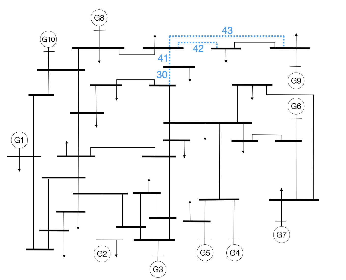
For line failures which minimally change the power flow solution, we approximate the resulting changes to the dynamics (LABEL:eq:powerDAE) as additive perturbations to ${G}$. For four line failures of interest, 30, 41, 42, and 43 (see Figure 2), we compute these perturbations $\Delta{G}_{30},\Delta{G}_{41},\Delta{G}_{42}$ and $\Delta{G}_{43}$. For instance, when line 43 fails the ODE (28) remains unchanged and the constraint (29) is modified to

$$0=\overline{F}\left[\begin{array}[]{c}\boldsymbol{d\delta}(t)\\ \boldsymbol{d\omega}(t)\end{array}\right]+(G+\Delta G_{43})\boldsymbol{v}(t).$$ (32)

5.1.2 Controller Design

We design a static linear controller, assuming access to relative angle measurements, e.g. $d\delta_{1}-d\delta_{2}$ and absolute angular velocity measurements, e.g. $d\omega_{1}$. Such a control policy will take the form [32]

$$\boldsymbol{u}(t)=K\boldsymbol{x}(t),$$ (33)

where $\boldsymbol{x}(t)=Q\left[\begin{array}[]{c}\boldsymbol{d\delta}(t)\\ \boldsymbol{d\omega}(t)\end{array}\right]$ is a reduced state vector and $Q$ is matrix whose columns form an orthonormal basis for the null space of $\left[\begin{array}[]{cc}\mathbb{1}^{\top}&0\end{array}\right]$. The corresponding reduced dynamics are

$$\dot{\boldsymbol{x}}(t){\small{=}}A\boldsymbol{x}(t)+B_{v}\boldsymbol{v}(t)+B_{w}(\boldsymbol{w}(t)+\boldsymbol{u}(t))$$ (34)

$$0=F\boldsymbol{x}(t)+G\boldsymbol{v}(t)$$

$$\boldsymbol{y}=C\boldsymbol{x}(t),$$

where $A=Q^{\top}\overline{A}Q,$ $B_{v}=Q^{\top}\overline{B}_{v},$ $B_{w}=Q^{\top}\left[\begin{array}[]{cc}0&I\end{array}\right]^{\top}$, $F=\overline{F}Q$ and $C=\overline{C}Q$. The input-output behavior of (LABEL:eq:powerDAE) is equivalent to that of the original system (28)-(30), due to property (31) and the unobservability of the removed mode from output $\boldsymbol{y}.$ Removal of this zero mode removes any implicit equality constraints in (LABEL:eq:powerDAE), which may cause numerical issues.

When (LABEL:eq:powerDAE) describes the nominal open-loop system, the dynamics of the system with line 43 removed and in feedback with control (33) are

$$\dot{\boldsymbol{x}}(t) =A_{\rm cl}\boldsymbol{x}(t)+B_{v}\boldsymbol{v}(t)+B_{w}\boldsymbol{w}(t)$$ (35a)

$$0 =F\boldsymbol{x}(t)+(G+\Delta G_{43})\boldsymbol{v}(t)$$ (35b)

$$\boldsymbol{y}(t) =C\boldsymbol{x}(t),$$ (35c)

where $A_{\rm cl}:=(A{\small+}B_{u}K)$. We choose $K$ to place all closed-loop eigenvalues in the half plane $\{z;~{}\Re(z)<-0.5\}$.

5.1.3 Uncertainty Characterization

Rather than confirmining dissipativity for line failures one-by-one, we prioritize computationally tractability as the number of line failures of interest grows and construct a (conservative) uncertainty set containing each contingency. Dissipativity is confirmed over this set through one LMI using Proposition 2. An added benefit of this approach is the implicit incorporation of robustness, and we will see that the conservatism introduced for our example is quite small.

To create this uncertainty set, we compute the differences $\Delta G_{i}\small{-}\Delta G_{43}$ for $i=30,41,42$. The magnitudes of the singular values of these differences drop off rapidly, and thus we approximate each by a “structured” [33] rank three matrix, where “structure” corresponds to preserving the physical property (31): $\Delta G_{41}\small{-}\Delta G_{43}=H_{1}J_{1}^{\top},\Delta G_{42}\small{-}\Delta G_{43}=H_{2}J_{2}^{\top},\Delta G_{30}\small{-}\Delta G_{43}=H_{3}J_{3}^{\top},$ with $H_{i},J_{i}\in\mathbb{R}^{78\times 3}.$ Then,

$$0=Fx+(G{\small+}\Delta G_{43})v+\sum_{i=1}^{3}\tfrac{1-\theta_{i}}{2}H_{i}J_{i}^{\top}v,$$ (36)

$\theta_{i}\in[-1,1]$, covers the algebraic constraint corresponding to each of the four line failures of interest, e.g., $\theta_{1}=\theta_{2}=\theta_{3}=1$ and $\theta_{1}=\small{-}1,\theta_{2}=\theta_{3}=0$ correspond to the removal of line 43 and 41, respectively. This uncertainty is incorporated as

$$\dot{\boldsymbol{x}}(t) =A_{\rm cl}B{x}(t)+B_{v}\boldsymbol{v}(t)+B_{w}\boldsymbol{w}(t),$$ (37)

$$0 =F\boldsymbol{x}(t)+G_{v}\boldsymbol{v}(t)+G_{\xi}\boldsymbol{\xi}(t),$$

$$\boldsymbol{y}(t) =C\boldsymbol{x}(t),$$

where

$$G_{\xi}{\small{=}}\left[\begin{array}[]{ccc}H_{1}&H_{2}&H_{3}\end{array}\right],$$ (38)

$$G_{v}{\small{=}}G{\small{+}}\Delta G_{43}{\small{+}}\tfrac{1}{2}\left(H_{1}J_{1}^{\top}{\small{+}}H_{2}J_{2}^{\top}{\small{+}}H_{3}J_{3}^{\top}\right)$$

and $\boldsymbol{\xi}(t)=\left[\begin{array}[]{ccc}\boldsymbol{\xi}_{1}(t)^{\top}&\boldsymbol{\xi}_{2}(t)^{\top}&\boldsymbol{\xi}_{3}(t)^{\top}\end{array}\right]^{\top}$ is the output of some $\Delta$ satisfying the pointwise quadratic constraints

$$\left[\begin{array}[]{c}\xi_{i}\\ v\end{array}\right]^{\top}\left[\begin{array}[]{cc}X_{i}&\frac{-1}{2}Y_{i}J_{i}^{\top}\\ \frac{-1}{2}J_{i}Y_{i}^{\top}&\frac{-1}{4}J_{i}X_{i}J_{i}^{\top}\end{array}\right]\left[\begin{array}[]{c}\xi_{i}\\ v\end{array}\right]\leq 0$$ (39)

for any $X_{i}=X_{i}^{\top}$ and $Y_{i}=-Y_{i}^{\top}$ [4].

Remark 5

This uncertainty set could be equivalently characterized by a polytopic set as in [12, Sec. 3]. Characterization (39) results in a lower dimensional LMI condition and allows us to incorporate the uncertainty set parameters $X_{i},Y_{i}$ as additional design variables for more flexibility.

5.2 $H_{\infty}$ Norm Bound over a set of Line Failures

We compute a bound on the $L_{2}$ gain from $\boldsymbol{w}$ to $\boldsymbol{y}$ of (37)-(LABEL:eq:power_uncertain2) with $\Delta$ satisfying (39) using Proposition 2. We formulate the corresponding convex optimization problem

$$\min_{P,\lambda,X_{1},Y_{1},X_{2},Y_{2},\gamma^{2}}~{}~{}~{}\gamma^{2}$$ (40)

$$~{}~{}~{}{\rm s.t.}~{}~{}P\succ 0,X_{i}=X_{i}^{\top},Y_{i}=-Y_{i}^{\top},\lambda\geq 0,$$

$$~{}~{}~{}~{}~{}~{}~{}~{}~{}\left[\begin{array}[]{cccc}A_{\rm{cl}}^{\top}P\small{+}PA_{\rm{cl}}\small{+}C^{\top}C&PB_{v}&0&PB_{w}\\ B_{v}^{\top}P&0&0&0\\ 0&0&0&0\\ B_{w}^{\top}P&0&0&-\gamma^{2}I\end{array}\right]$$

$$~{}~{}~{}~{}~{}~{}~{}~{}~{}~{}\preceq\lambda\left[\begin{array}[]{c}F^{\top}\\ G_{v}^{\top}\\ G_{\xi}^{\top}\\ 0\end{array}\right]\left[\begin{array}[]{cccc}F&G_{v}&G_{\xi}&0\end{array}\right]~{}+$$

$$~{}~{}~{}~{}~{}~{}~{}~{}~{}~{}~{}\left[\begin{array}[]{cccc}0&0&0&0\\ 0&\frac{-1}{4}\sum_{i=1}^{3}\left(J_{i}X_{i}J_{i}^{\top}\right)&W&0\\ 0&W^{\top}&X&0\\ 0&0&0&0\end{array}\right]$$

where $W:=\frac{-1}{2}\left[\begin{array}[]{ccc}J_{1}Y_{1}^{\top}&J_{2}Y_{2}^{\top}&J_{3}Y_{3}^{\top}\end{array}\right]$ and $X$ is the block diagonal matrix of $\{X_{1},X_{2},X_{3}\}.$ We solve (LABEL:eq:power_exmp_opt) numerically in MATLAB using CVX [34] with the SeDuMi solver [24] resulting in an $L_{2}$ gain bound of $\gamma=2.31$ over the uncertainty set. To evaluate conservatism, we compute the $L_{2}$ gain corresponding to each of the four line removals:

Line removed	30	41	42	43
$\begin{array}[]{c}\text{Closed-loop}\\ H_{\infty}\text{-norm}\end{array}$	2.215	2.222	2.219	2.217

We compute $L_{2}$ gains over the full uncertainty set via a grid search - the maximum value obtained is 2.2719, occurring at $\theta_{1}=0.1,\theta_{2}=0,\theta_{3}=0$ in (36); note that this point does not correspond to a physical line removal. Our bound $\gamma=2.31$ is 3.98% over the true maximal $L_{2}$ gain over the four line removals of interest and 1.68% over true bound for the full uncertainty set. Thus, for this case study, neither the choice of a larger uncertainty set nor the restriction to a single storage function (see Remark 2) cause much conservatism.

6 Conclusion

A general framework for analyzing dissipativity of DAE systems with uncertainties described by IQCs was provided. It was shown that dissipativity could be confirmed numerically in the case of polynomial or linear dynamics. Analysis of the IEEE 39-bus power system subject to line failures provided a case study. The sufficient condition for dissipativity derived introduces conservatism. This conservatism was insignificant in the presented case study; quantifying or minimizing this conservatism are potential extensions of this work.

Appendix

6.1 Proof of Proposition 1

By the lossless s-procedure (see, e.g., [35]), the existence of $\lambda\geq 0$ satisfying (LABEL:eq:lin_proof_lmi) is equivalent to nonpositivity of

$$\left[\begin{array}[]{c}x\\ v\\ w\end{array}\right]^{\top}\left[\begin{array}[]{c}F^{\top}\\ G_{v}^{\top}\\ G_{w}^{\top}\end{array}\right]\left[\begin{array}[]{ccc}F&G_{v}&G_{w}\end{array}\right]\left[\begin{array}[]{c}x\\ v\\ w\end{array}\right]$$ (41)

implying

$$\left[\begin{array}[]{c}x\\ v\\ w\end{array}\right]^{\top}\Bigg{(}\left[\begin{array}[]{ccc}A^{\top}P+PA&PB_{v}&PB_{w}\\ B_{v}^{\top}P&0&0\\ B_{w}^{\top}P&0&0\end{array}\right]$$ (42)

$$~{}~{}~{}~{}~{}~{}~{}~{}~{}~{}~{}-\left[\begin{array}[]{ccc}X_{xx}&0&X_{xw}\\ 0&0&0\\ X_{xw}^{\top}&0&X_{ww}\end{array}\right]\Bigg{)}\left[\begin{array}[]{c}x\\ v\\ w\end{array}\right]\leq 0.$$

Since $V(\cdot)$ is quadratic, and thus continuously differentiable, dissipativity (Definition 1) with $\boldsymbol{\xi}=0$ can be confirmed through an equivalent differential characterization that for all $x,v,w$ we have that

$$0=g(x,v,w,0)~{}\Rightarrow~{}\triangledown V(x)^{\top}f(x,v,w,0)\leq 0.$$

Nonpositivity of (41) is equivalent to $0=g(x,v,w,0)$ for linear $g$ of the form (16b), and condition $\triangledown V(x)^{\top}f(x,v,w,0)\leq 0$ reduces to (LABEL:eq:lin_diss_LMI) for linear $f$ of form (16a) and quadratic $V$. $\blacksquare$

6.2 Proof of Theorem 2:

Assume (LABEL:linear_thm_eq) holds, and left and right the inequality by $\left[\begin{array}[]{ccccc}x^{\top}&v^{\top}&\xi^{\top}&w^{\top}&\psi^{\top}\end{array}\right]$ and its transpose to arrive at

$$x^{\top}P(Ax+B_{v}v+B_{w}w+B_{\xi}\xi)+(\star)^{\top}Px+$$

$$\psi^{\top}P_{\Delta}\Big{(}A_{\psi}^{\top}\psi(t)\small{+}B_{\psi}{\small{\left[\begin{array}[]{c}x(t)\\ v(t)\\ \xi(t)\end{array}\right]}}\Big{)}+(\star)^{\top}P_{\Delta}\psi(t)$$

$$\leq\left[\begin{array}[]{c}x\\ w\end{array}\right]^{\top}\left[\begin{array}[]{cc}X_{xx}&X_{xw}\\ X_{xw}^{\top}&X_{ww}\end{array}\right]\left[\begin{array}[]{c}x\\ w\end{array}\right]$$

$$+\lambda\left[\begin{array}[]{c}x\\ v\\ \xi\\ w\end{array}\right]^{\top}\left[\begin{array}[]{c}F^{\top}\\ G_{v}^{\top}\\ G_{\xi}^{\top}\\ G_{w}^{\top}\end{array}\right]\left[\begin{array}[]{cccc}F&G_{v}&G_{\xi}&G_{w}\end{array}\right]\left[\begin{array}[]{c}x\\ v\\ \xi\\ w\end{array}\right]$$

$$+\tau\Big{(}C_{\psi}\psi+D_{\psi}{\small{\left[\begin{array}[]{c}x\\ v\\ \xi\end{array}\right]}}\Big{)}^{\top}M\Big{(}C_{\psi}\psi+D_{\psi}{\small{\left[\begin{array}[]{c}x\\ v\\ \xi\end{array}\right]}}\Big{)},$$

where each of the terms $(\star)$ may be inferred by symmetry; this is condition (LABEL:eq:nonlinear_general_int) for dissipativity in the linear setting so that the result follows immediately from Theorem 1. $\blacksquare$

6.3 Power Network Model Parameters:

The ODE parameters are given by

$$\overline{A}=\left[\begin{array}[]{cc}0_{n_{g}\times n_{g}}&\Omega\cdot I_{n_{g}}\\ {\rm diag}(\frac{-E\circ V_{G}\circ\cos(\delta-\theta_{G})}{2H\circ X_{d}})&{\rm diag}(\frac{-D}{2H})\end{array}\right]$$

$$\overline{B}=\left[\begin{array}[]{cccc}0_{n_{g}\times n_{g}}&0_{n_{g}\times n_{g}}&0_{n_{g}\times n_{l}}&0_{n_{g}\times n_{l}}\\ \overline{B}_{21}&\overline{B}_{22}&0_{n_{g}\times n_{l}}&0_{n_{g}\times n_{l}}\end{array}\right],$$

where $\small{\overline{B}_{21}={\rm diag}\left(\frac{-E\circ\sin(\delta-\theta_{G})}{2H\circ X_{d}}\right)}$, and $\small{\overline{B}_{22}={\rm diag}\left(\frac{E\circ V_{G}\circ\cos(\delta-\theta_{G})}{2H\circ X_{d}}\right)}.$

To define $\overline{F}$ and $G$, we decompose the following matrices into real and imaginary parts:

$$Y_{d}=Y^{d}_{\rm re}+iY^{d}_{\rm im},$$

$$Y^{G}=\left[\begin{array}[]{c}Y_{11}+Y_{d}\\ Y_{21}\end{array}\right]=Y^{G}_{\rm re}+iY^{G}_{\rm im},$$

$$Y^{L}=\left[\begin{array}[]{c}Y_{12}\\ Y_{22}+Y_{L}\end{array}\right]=Y^{L}_{\rm re}+iY^{L}_{\rm im}.$$

With this notation,

$$\overline{F}=\left[\begin{array}[]{cc}Y^{d}_{\rm im}\cdot{\rm diag}(E\circ\cos(\delta)&0_{n_{g}\times n_{g}}\\ 0_{n_{l}\times n_{g}}&0_{n_{l}\times n_{g}}\\ Y^{d}_{\rm im}\cdot{\rm diag}(E\circ\sin(\delta)&0_{n_{g}\times n_{g}}\\ 0_{n_{l}\times n_{g}}&0_{n_{l}\times n_{g}}\end{array}\right]$$

$${G}=\left[\begin{array}[]{cccc}G_{V_{G}}&G_{\theta_{G}}&G_{V_{L}}&G_{\theta_{L}}\end{array}\right],$$

where

$${\small{G_{V_{G}}=\left[\begin{array}[]{c}Y^{G}_{\rm re}\cdot{\rm diag}(\cos\theta_{G})-Y^{G}_{\rm im}\cdot{\rm diag}(\sin\theta_{G})\\ Y^{G}_{\rm re}\cdot{\rm diag}(\sin\theta_{G})+Y^{G}_{\rm im}\cdot{\rm diag}(\cos\theta_{G})\end{array}\right]}}$$

$$G_{\theta_{G}}=$$

$$\small{\left[\begin{array}[]{c}\small{-}Y^{G}_{\rm re}\cdot{\rm diag}\left(V_{G}\circ\sin\theta_{G}\right)\small{-}Y^{G}_{\rm im}\cdot{\rm diag}(V_{G}\circ\cos\theta_{G})\\ Y^{G}_{\rm re}\cdot{\rm diag}\left(V_{G}\circ\cos\theta_{G}\right)\small{-}Y^{G}_{\rm im}\cdot{\rm diag}\left(V_{G}\circ\sin\theta_{G}\right)\end{array}\right]}$$

$${\small{G_{V_{L}}=\left[\begin{array}[]{c}Y^{L}_{\rm re}\cdot{\rm diag}\left(\cos\theta_{L}\right)-Y^{L}_{\rm im}\cdot{\rm diag}\left(\sin\theta_{L}\right)\\ Y^{L}_{\rm re}\cdot{\rm diag}\left(\sin\theta_{L}\right)+Y^{L}_{\rm im}\cdot{\rm diag}\left(\cos\theta_{L}\right)\end{array}\right]}}$$

$${\small G_{\theta_{L}}=}$$

$${\small{\left[\begin{array}[]{c}\small{-}Y^{L}_{\rm re}\cdot{\rm diag}\left(V_{L}\circ\sin\theta_{L}\right)\small{-}Y^{L}_{\rm im}\cdot{\rm diag}\left(V_{L}\circ\cos\theta_{L}\right)\\ Y^{L}_{\rm re}\cdot{\rm diag}\left(V_{L}\circ\cos\theta_{L}\right)-Y^{L}_{\rm im}\cdot{\rm diag}\left(V_{L}\circ\sin\theta_{L}\right)\end{array}\right]}}$$

[]Emily Jensen is a postdoctoral researcher at UC Berkeley and previously held a postdoctoral appointment at Northeastern University. She received her B.S. in Engineering, Mathematics & Statistics from UC Berkeley in 2015 and the Ph.D. degree in Electrical & Computer Engineering from the University of California, Santa Barbara in 2020. She was a research & instructional assistant at Caltech in 2016. Dr. Jensen received the UC Regents’ Graduate Fellowship (2016), the Zonta Amelia Earhart Fellowship (2019) and an honorable mention for the Young Author Award at the IFAC Conference on Networked Systems (2022). []Neelay Junnarkar is a Ph.D. student at UC Berkeley and previously received a B.S. in Electrical Engineering and Computer Sciences from UC Berkeley (2021). He worked as an intern with Siemens Technology in 2023. His research interests include applications of machine learning to control theory. []Murat Arcak is a professor at U.C. Berkeley in the Electrical Engineering and Computer Sciences Department, with a courtesy appointment in Mechanical Engineering. He received the B.S. degree in Electrical Engineering from the Bogazici University, Istanbul, Turkey (1996) and the M.S. and Ph.D. degrees from the University of California, Santa Barbara (1997 and 2000). He received a CAREER Award from the National Science Foundation in 2003, the Donald P. Eckman Award from the American Automatic Control Council in 2006, the Control and Systems Theory Prize from the Society for Industrial and Applied Mathematics (SIAM) in 2007, and the Antonio Ruberti Young Researcher Prize from the IEEE Control Systems Society in 2014. He is a member of ACM and SIAM, and a fellow of IEEE and the International Federation of Automatic Control (IFAC).

[]Xiaofan Wu received the B.Eng. degree in detection guidance and control technology from the Beijing University of Aeronautics and Astronautics, Beijing, China, in 2010, and the M.S. and Ph.D. degrees in electrical engineering from the University of Minnesota, Minneapolis, MN, USA, in 2012 and 2016, respectively. He is currently the Head of Research Group - Autonomous System and Control with Siemens Technology in Princeton, NJ, USA. He is also a Project Manager for the Siemens Princeton Island Grid Living Lab. He has more than ten years of experience in modeling, control and optimization of energy systems and smart grids. He was a Visiting Scholar with the Automatic Control Laboratory, ETH Zurich, Switzerland, from March to June 2016. He was the recipient of the 2021 Thomas Edison Patent Award of the New Jersey R&D Council.

[]Suat Gumussoy is a senior key expert on data-driven control at Autonomous Systems & Control group at Siemens Technology in Princeton, NJ. His general research interests are learning, control, and autonomous systems with particular focus on reinforcement learning, data-driven modeling and control, and development of commercial engineering design tools.

Dr. Gumussoy received his B.S. degrees in Electrical & Electronics Engineering and Mathematics from Middle East Technical University at Turkey in 1999 and M.S., Ph.D. degrees in Electrical and Computer Engineering from The Ohio State University at USA in 2001 and 2004. He worked as a system engineer in defense industry (2005-2007) and he was a postdoctoral associate in Computer Science Department at KU Leuven (2008-2011). He was a principal control system engineer in Controls & Identification Team at MathWorks where his contributions ranges from state-of-the-art numerical algorithms to comprehensive analysis & design tools in Control System, Robust Control, System Identification and Reinforcement Learning Toolboxes.

He served as an Associate Editor in IEEE Transactions on Control Systems Technology and IEEE Conference Editorial Board for 2018-2022. He is a Senior Member of IEEE and a member of IFAC Technical Committee on Linear Control Systems.

References

- [1] J. C. Willems, “Dissipative dynamical systems part I: General theory,” Archive for rational mechanics and analysis, vol. 45, no. 5, pp. 321–351, 1972.
- [2] R. Lozano, B. Brogliato, O. Egeland, and B. Maschke, Dissipative systems analysis and control: theory and applications. Springer Science & Business Media, 2013.
- [3] B. Hu, M. J. Lacerda, and P. Seiler, “Robustness analysis of uncertain discrete-time systems with dissipation inequalities and integral quadratic constraints,” International Journal of Robust and Nonlinear Control, vol. 27, no. 11, pp. 1940–1962, 2017.
- [4] A. Megretski and A. Rantzer, “System analysis via integral quadratic constraints,” IEEE transactions on automatic control, vol. 42, no. 6, pp. 819–830, 1997.
- [5] A. Kumar and P. Daoutidis, Control of nonlinear differential algebraic equation systems with applications to chemical processes, vol. 397. CRC Press, 1999.
- [6] U. M. Ascher and L. R. Petzold, Computer methods for ordinary differential equations and differential-algebraic equations, vol. 61. Siam, 1998.
- [7] E. Yip and R. Sincovec, “Solvability, controllability, and observability of continuous descriptor systems,” IEEE transactions on Automatic Control, vol. 26, no. 3, pp. 702–707, 1981.
- [8] Y. Feng and M. Yagoubi, Robust control of linear descriptor systems. Springer, 2017.
- [9] M. Darouach and M. Boutayeb, “Design of observers for descriptor systems,” IEEE transactions on Automatic Control, vol. 40, no. 7, pp. 1323–1327, 1995.
- [10] D. Chu and R. C. Tan, “Algebraic characterizations for positive realness of descriptor systems,” SIAM Journal on Matrix Analysis and Applications, vol. 30, no. 1, pp. 197–222, 2008.
- [11] P. Liu, Q. Zhang, X. Yang, and L. Yang, “Passivity and optimal control of descriptor biological complex systems,” IEEE Transactions on Automatic Control, vol. 53, no. Special Issue, pp. 122–125, 2008.
- [12] E. Uezato and M. Ikeda, “Strict LMI conditions for stability, robust stabilization, and h/sub/spl infin//control of descriptor systems,” in Proceedings of the 38th IEEE Conference on Decision and Control (Cat. No. 99CH36304), vol. 4, pp. 4092–4097, IEEE, 1999.
- [13] F. E. Udwadia and P. Phohomsiri, “Explicit equations of motion for constrained mechanical systems with singular mass matrices and applications to multi-body dynamics,” Proceedings of the Royal Society A: Mathematical, Physical and Engineering Sciences, vol. 462, no. 2071, pp. 2097–2117, 2006.
- [14] H. Choi, P. J. Seiler, and S. V. Dhople, “Propagating uncertainty in power-system dae models with semidefinite programming,” IEEE Transactions on Power Systems, vol. 32, no. 4, pp. 3146–3156, 2017.
- [15] L. E. Ghaoui, F. Gu, B. Travacca, A. Askari, and A. Y. Tsai, “Implicit deep learning,” 2020.
- [16] F. Dorfler and F. Bullo, “Kron reduction of graphs with applications to electrical networks,” IEEE Transactions on Circuits and Systems I: Regular Papers, vol. 60, no. 1, pp. 150–163, 2012.
- [17] J.-Y. Lin and Z.-H. Yang, “Existence and uniqueness of solutions for non-linear singular (descriptor) systems,” International journal of systems science, vol. 19, no. 11, pp. 2179–2184, 1988.
- [18] S. Reich, “On an existence and uniqueness theory for nonlinear differential-algebraic equations,” Circuits, Systems and Signal Processing, vol. 10, pp. 343–359, 1991.
- [19] P. J. Rabier and W. C. Rheinboldt, “A geometric treatment of implicit differential-algebraic equations,” Journal of Differential Equations, vol. 109, no. 1, pp. 110–146, 1994.
- [20] W. C. Rheinboldt, “Differential-algebraic systems as differential equations on manifolds,” Mathematics of computation, vol. 43, no. 168, pp. 473–482, 1984.
- [21] S. L. Campbell and E. Griepentrog, “Solvability of general differential algebraic equations,” SIAM Journal on Scientific Computing, vol. 16, no. 2, pp. 257–270, 1995.
- [22] P. Seiler, A. Packard, and G. J. Balas, “A dissipation inequality formulation for stability analysis with integral quadratic constraints,” in 49th IEEE Conference on Decision and Control (CDC), pp. 2304–2309, IEEE, 2010.
- [23] S. Prajna, A. Papachristodoulou, and P. A. Parrilo, “Introducing sostools: A general purpose sum of squares programming solver,” in Proceedings of the 41st IEEE Conference on Decision and Control, 2002., vol. 1, pp. 741–746, IEEE, 2002.
- [24] J. F. Sturm, “Using SeDuMi 1.02, a MATLAB toolbox for optimization over symmetric cones,” Optimization methods and software, vol. 11, no. 1-4, pp. 625–653, 1999.
- [25] J. Buch, S.-C. Liao, and P. Seiler, “Robust control barrier functions with sector-bounded uncertainties,” IEEE Control Systems Letters, vol. 6, pp. 1994–1999, 2021.
- [26] H. Hindi and S. Boyd, “Analysis of linear systems with saturation using convex optimization,” in Proceedings of the 37th IEEE conference on decision and control (Cat. No. 98CH36171), vol. 1, pp. 903–908, IEEE, 1998.
- [27] S. Bai, J. Z. Kolter, and V. Koltun, “Deep equilibrium models,” 2019.
- [28] N. Junnarkar, H. Yin, F. Gu, M. Arcak, and P. Seiler, “Synthesis of stabilizing recurrent equilibrium network controllers,” in 2022 IEEE 61st Conference on Decision and Control (CDC), pp. 7449–7454, IEEE, 2022.
- [29] N. Xue, X. Wu, S. Gumussoy, U. Muenz, A. Mesanovic, C. Heyde, Z. Dong, G. Bharati, S. Chakraborty, L. Cockcroft, et al., “Dynamic security optimization for N-1 secure operation of hawaii island system with 100% inverter-based resources,” IEEE Transactions on Smart Grid, vol. 13, no. 5, pp. 4009–4021, 2021.
- [30] T. Athay, R. Podmore, and S. Virmani, “A practical method for the direct analysis of transient stability,” IEEE Transactions on Power Apparatus and Systems, no. 2, pp. 573–584, 1979.
- [31] J. H. Chow and J. J. Sanchez-Gasca, Power system modeling, computation, and control. John Wiley & Sons, 2020.
- [32] X. Wu, F. Dörfler, and M. R. Jovanović, “Input-output analysis and decentralized optimal control of inter-area oscillations in power systems,” IEEE Transactions on Power Systems, vol. 31, no. 3, pp. 2434–2444, 2015.
- [33] M. T. Chu, R. E. Funderlic, and R. J. Plemmons, “Structured low rank approximation,” Linear algebra and its applications, vol. 366, pp. 157–172, 2003.
- [34] M. Grant and S. Boyd, “CVX: MATLAB software for disciplined convex programming, version 2.1.” urlhttp://cvxr.com/cvx, Mar. 2014.
- [35] S. Boyd, S. P. Boyd, and L. Vandenberghe, Convex optimization. Cambridge university press, 2004.