LLM4TS: Aligning Pre-Trained LLMs as Data-Efficient Time-Series Forecasters

Abstract

Multivariate time-series forecasting is vital in various domains, e.g., economic planning and weather prediction. Deep train-from-scratch models have exhibited effective performance yet require large amounts of data, which limits real-world applicability. Recently, researchers have leveraged the representation learning transferability of pre-trained Large Language Models (LLMs) to handle limited non-linguistic datasets effectively. However, incorporating LLMs with time-series data presents challenges of limited adaptation due to different compositions between time-series and linguistic data, and the inability to process multi-scale temporal information. To tackle these challenges, we propose LLM4TS, a framework for time-series forecasting with pre-trained LLMs. LLM4TS consists of a two-stage fine-tuning strategy: the time-series alignment stage to align LLMs with the nuances of time-series data, and the forecasting fine-tuning stage for downstream time-series forecasting tasks. Furthermore, our framework features a novel two-level aggregation method that integrates multi-scale temporal data within pre-trained LLMs, enhancing their ability to interpret time-specific information. In experiments across 7 time-series forecasting datasets, LLM4TS is superior to existing state-of-the-art methods compared with trained-from-scratch models in full-shot scenarios, and also achieves an average improvement of $6.84\%$ in MSE in few-shot scenarios. In addition, evaluations compared with different self-supervised learning approaches highlight LLM4TS’s effectiveness with representation learning in forecasting tasks.

1 Introduction

Forecasting is a vital task in multivariate time-series analysis, not only for its ability to operate without manual labeling but also for its importance in practical applications such as economic planning Lai et al. (2018) and weather prediction Zhou et al. (2021). Recently, numerous deep train-from-scratch models have been developed for time-series forecasting Nie et al. (2023), although some lean towards unsupervised representation learning Chang et al. (2023) and transfer learning Zhang et al. (2022); Zhou et al. (2023). Generally, these approaches aim to employ adept representation learners: first extracting rich representations from the time-series data and then using these representations for forecasting.

Achieving an adept representation learner requires sufficient training data Hoffmann et al. (2022), yet in real-world scenarios, there is often a lack of large-scale time-series datasets. For instance, in industrial manufacturing, the sensor data for different products cannot be combined for further analysis, leading to limited data for each product type Yeh et al. (2019). Recent research has pivoted towards pre-trained LLMs in Natural Language Processing (NLP) Radford et al. (2019); Touvron et al. (2023) , exploiting their robust representation learning and few-shot learning capabilities. Moreover, these LLMs can adapt to non-linguistic datasets (e.g., images Lu et al. (2021), audio Ghosal et al. (2023), tabular data Hegselmann et al. (2023), and time-series data Zhou et al. (2023)) by fine-tuning with only a few parameters and limited data. While LLMs are renowned for their exceptional transfer learning capabilities across various fields, the domain-specific nuances of time-series data introduce two challenges in leveraging these models for time-series forecasting.

The first challenge of employing LLMs for time-series forecasting is their limited adaptation to the unique characteristics of time-series data due to LLMs’ initial pre-training focus on the linguistic corpus. While LLMs have been both practically and theoretically proven Zhou et al. (2023) to be effective in transfer learning across various modalities thanks to their data-independent self-attention mechanism, their primary focus on general text during pre-training causes a shortfall in recognizing key time-series patterns and nuances crucial for accurate forecasting. This limitation is evident in areas such as meteorology and electricity forecasting Zhou et al. (2021), where failing to account for weather patterns and energy consumption trends leads to inaccurate predictions.

The second challenge lies in the limited capacity to process multi-scale temporal information. While LLMs are adept at understanding the sequence and context of words, they struggle to understand temporal information due to the lack of utilizing multi-scale time-related data such as time units (e.g., seconds, minutes, hours, etc.) and specific dates (e.g., holidays, significant events). This temporal information is vital in time-series analysis for identifying and predicting patterns Wu et al. (2021); for instance, in energy management, it is used to address consumption spikes during daytime and in summer/winter, in contrast to the lower demand during the night and in milder seasons Zhou et al. (2021). This underscores the importance of models adept at interpreting multi-scale temporal patterns (hourly to seasonal) for precise energy demand forecasting. However, most LLMs (e.g., Radford et al. (2019); Touvron et al. (2023)) built on top of the Transformer architecture do not naturally incorporate multi-scale temporal information, leading to models that fail to capture crucial variations across different time scales.

To address the above issues, we propose LLM4TS, a framework for time-series forecasting with pre-trained LLMs. Regarding the first challenge, our framework introduces a two-stage fine-tuning approach: the time-series alignment stage and the forecasting fine-tuning stage. The first stage focuses on aligning the LLMs with the characteristics of time-series data by utilizing the autoregressive objective, enabling the fine-tuned LLMs to adapt to time-series representations. The second stage is incorporated to learn corresponding time-series forecasting tasks. In this manner, our model supports effective performance in full- and few-shot scenarios. Notably, throughout both stages, most parameters in the pre-trained LLMs are frozen, thus preserving the model’s inherent representation learning capability. To overcome the limitation of LLMs in integrating multi-scale temporal information, we introduce a novel two-level aggregation strategy. This approach embeds multi-scale temporal information into the patched time-series data, ensuring that each patch not only represents the series values but also encapsulates the critical time-specific context. Consequently, LLM4TS emerges as a data-efficient time-series forecaster, demonstrating robust few-shot performance across various datasets (Figure 1).

In summary, the paper’s main contributions are as follows:

• Aligning LLMs Toward Time-Series Data: To the best of our knowledge, LLM4TS is the first method that aligns pre-trained Large Language Models with time-series characteristics, effectively utilizing existing representation learning and few-shot learning capabilities.

• Multi-Scale Temporal Information in LLMs: To adapt to time-specific information, a two-level aggregation method is proposed to integrate multi-scale temporal data within pre-trained LLMs.

• Robust Performance in Forecasting: LLM4TS excels in 7 real-world time-series forecasting benchmarks, outperforming state-of-the-art methods, including those trained from scratch. It also demonstrates strong few-shot capabilities, particularly with only $5\%$ of data, where it surpasses the best baseline that uses $10\%$ of data. This efficiency makes LLM4TS highly relevant for practical, real-world forecasting applications.

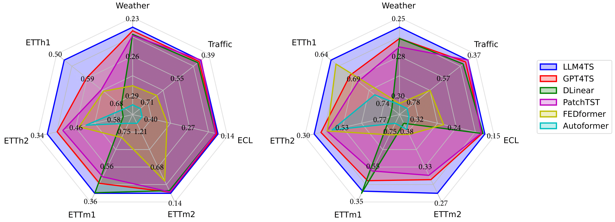
(a) 10% training data

(b) 5% training data

Figure 1: Model performance comparison on few-shot forecasting.

2 Related Work

2.1 Transfer Learning Across Various Modalities with LLMs

LLMs have demonstrated their effectiveness in transfer learning across a variety of modalities, such as images Lu et al. (2021), audio Ghosal et al. (2023), tabular data Hegselmann et al. (2023), and time-series data Zhou et al. (2023). A key motivation for employing LLMs in various modalities is their ability to achieve notable performance with limited data Zhou et al. (2023). To preserve their data-independent representation learning capability, most parameters in these LLMs are kept fixed. Empirical evidence Lu et al. (2021); Zhou et al. (2023) indicates that LLMs keeping most parameters unchanged often outperform those trained from scratch, underscoring the value of maintaining these models’ pre-existing representation learning strengths. Theoretically, it is shown that the self-attention modules in these pre-trained transformers develop the capacity for data-independent operations (akin to principal component analysis Zhou et al. (2023)), enabling them to function effectively as universal compute engines Lu et al. (2021) or general computation calculators Giannou et al. (2023). In the time-series domain, GPT4TS Zhou et al. (2023) utilizes the pre-trained GPT-2 and demonstrates strong performance in time-series forecasting under few-shot conditions without modifying most parameters. With our LLM4TS, we address the challenges of limited adaptation to time-series characteristics and the difficulty in processing multi-scale temporal information, thereby enhancing performance in time-series forecasting.

2.2 Long-term Time-Series Forecasting

Numerous efforts have been dedicated to employing Transformer models for long-term time-series forecasting Zhou et al. (2021); Wu et al. (2021); Zhou et al. (2022); Nie et al. (2023). While Transformer-based models have gained traction, DLinear Zeng et al. (2023) reveals that a single-layer linear model can surpass many of these sophisticated Transformer-based approaches. These deep train-from-scratch models exhibit outstanding performance when trained on sufficient datasets, but their efficacy decreases in limited-data scenarios. In contrast, LLM4TS sets new benchmarks alongside these state-of-the-art approaches in both full- and few-shot scenarios.

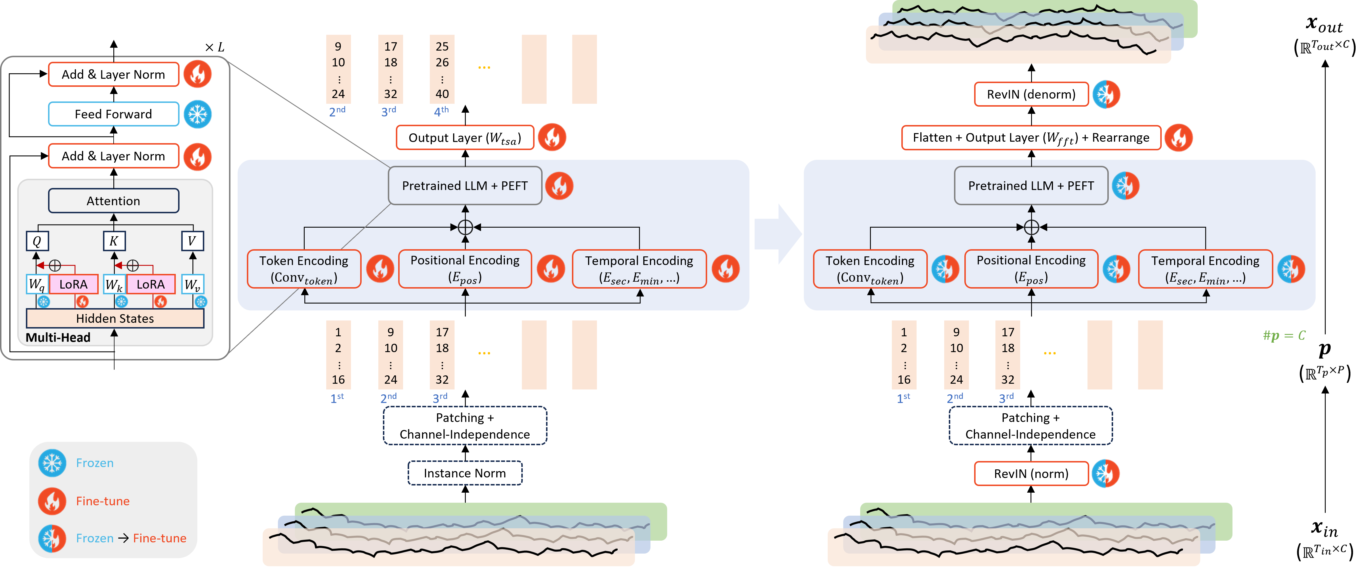
(a) Time-Series Alignment

(b) Forecasting Fine-Tuning

Figure 2: LLM4TS framework. The numbers in the patched time series (e.g., 1, 2, …, 16 in the first patch) indicate the sequential order of the timestamps. The framework consists of two stages: (a) Time-series alignment, which uses the autoregressive approach to align the pre-trained LLM with patched time-series data. (b) Forecasting fine-tuning, which starts with linear probing (i.e., only the output layer is unfrozen), followed by full fine-tuning (all the layers and PEFT components in the LLM are unfrozen).

2.3 Time-Series Representation Learning

In the time-series domain, self-supervised learning emerges as a prominent approach to representation learning. While Transformers are widely recognized as prime candidates for end-to-end time-series analysis Xu et al. (2021); Liu et al. (2021); Nie et al. (2023), CNN-based Yue et al. (2022) or RNN-based Tonekaboni et al. (2021) backbones consistently stand out as the preferred architecture in time-series self-supervised learning. However, the inherent capability of Transformers to model long-range dependencies and capture patterns aligns perfectly with time-series data, which involve complex sequential relationships. Since the time-series alignment stage in LLM4TS can be seen as a self-supervised learning approach, we evaluate LLM4TS’s representation learning capability and demonstrate the full potential of Transformers in self-supervised learning, surpassing the performance of conventional CNN and RNN-based models.

3 Problem Formulation

Given a complete and evenly-sampled multivariate time series, we use a sliding data window to extract sequential samples. This window moves with a stride of $1$ and has a total length of $T_{in}+T_{out}$ — comprising past data $\textbf{x}_{in}=(d_{1},\dots,d_{T_{in}})$ with a look-back window length $T_{in}$ and future data $\textbf{x}_{out}=(d_{T_{in}+1},\dots,d_{T_{in}+T_{out}})$ with a prediction length $T_{out}$. For each time step $t$, $d_{t}$ represents a $C$-dimensional vector, where $C$ denotes the number of features. Our objective is to use the past data $\textbf{x}_{in}\in\mathbb{R}^{T_{in}\times C}$ to predict the future data $\textbf{x}_{out}\in\mathbb{R}^{T_{out}\times C}$.

4 The Proposed LLM4TS

Figure 2 illustrates our LLM4TS framework, leveraging the pre-trained GPT-2 Radford et al. (2019) as the backbone model. We first introduce the time-series alignment stage, which focuses on aligning the LLMs with the characteristics of time-series data using an autoregressive objective (Section 4.1). Subsequently, the forecasting fine-tuning stage is designed to further enhance the model’s ability to handle time-series forecasting tasks (Section 4.2).

4.1 Time-Series Alignment

Existing LLMs are pre-trained on a general language corpus, which means they fail to learn contextualized information outside linguistic domains; therefore, the time-series alignment stage is proposed to align LLMs with the characteristics of time-series data. Given our selection of GPT-2 Radford et al. (2019) as the backbone model, which is a causal language model, we ensure that this stage adopts the same autoregressive training methodology used during its pre-training phase. Figure 2(a) illustrates the autoregressive objective in the time-series alignment stage: given an input sequence of patched time-series data (e.g., $1^{st}$ patch, $2^{nd}$ patch, $3^{rd}$ patch, etc.), the backbone model generates an output sequence shifted one patch to the right (e.g., $2^{nd}$ patch, $3^{rd}$ patch, $4^{th}$ patch, etc.).

Instance Normalization

Data normalization is essential for stable performance when adapting pre-trained models across various modalities. Alongside the layer normalization used in the pre-trained LLM, we incorporate instance normalization to improve consistency and reliability in handling diverse time-series datasets. In our model, instance normalization is employed without incorporating a trainable affine transformation. This is crucial because when a batch of data is gathered and instance normalization is applied with a trainable affine transformation, the resulting transformed data becomes unsuitable to be the ground truth for the output. Given that an autoregressive objective is used at this stage, applying a trainable affine transformation is not feasible.

Given an input time-series sample $\textbf{x}_{in}\in\mathbb{R}^{T_{in}\times C}$, we apply instance normalization (IN) to produce a normalized time-series sample $\textbf{x}_{normed}\in\mathbb{R}^{T_{in}\times C}$ with zero mean and unit standard deviation:

$$\textbf{x}_{normed}=\text{IN}(\textbf{x}_{in}).$$ (1)

Time-Series Tokenization

The context window sizes in pre-trained LLMs (e.g., 1024 in GPT-2) are sufficient for NLP tasks but are inadequate for long-term time-series forecasting. In our experiments, a prediction length of 720 combined with a look-back window size of 512 easily exceeds these limits. To address this, we adopt channel-independence along with patching Nie et al. (2023) for time-series tokenization, effectively resolving the context window size constraint and simultaneously reducing the time and space complexity of the Transformer quadratically. Channel-independence converts multivariate time-series data into multiple univariate time-series data, thus transforming the data’s dimension to $\mathbb{R}^{T_{in}\times 1}$, with the channel dimension $C$ merged into the batch size dimension. The subsequent patching step groups adjacent time steps into a singular patch-based token, reducing the input sample’s time dimension from $T_{in}$ to $T_{p}$, where $T_{p}$ denotes the number of patches, and concurrently expanding the feature dimension from $1$ to $P$, with $P$ representing the patch length.

Given a normalized time-series sample $\textbf{x}_{normed}\in\mathbb{R}^{T_{in}\times C}$, we first apply channel-independence (CI), and then patching to produce a series of patches $\textbf{p}\in\mathbb{R}^{T_{p}\times P}$:

$$\textbf{p}=\text{patching}(\text{CI}(\textbf{x}_{normed})).$$ (2)

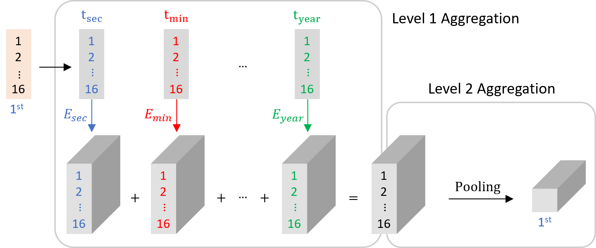
Figure 3: Temporal encoding for patched time-series data involves a two-level aggregation process. Here, only the first patch is shown for simplicity; in practice, all patches in a batch are processed simultaneously. Level 1 aggregation calculates the temporal embedding for each time unit and sums them together. Next, Level 2 aggregation applies a pooling method to extract the final temporal embedding.

Three Encodings for Patched Time-Series Data

Given our goal to adapt a pre-trained LLM for time-series data, the original token encoding layer (designed for text) becomes unsuitable due to the mismatched modalities. Additionally, we design a new temporal encoding layer to address the inability to process multi-scale temporal information.

Given a series of tokens, applying token encoding is necessary to align their dimensions with the latent embedding dimension of the pre-trained LLM. In standard NLP practices, this encoding uses a trainable lookup table to map tokens into a high-dimensional space. However, this method only suits scalar tokens, whereas our patched time-series data are vectors. Therefore, we drop the original token encoding layer in the LLM, and employ a one-dimensional convolutional layer $\text{Conv}_{token}$ as our new token encoding layer. As opposed to employing a linear layer Zhou et al. (2023), we choose a convolutional layer due to its superior ability to retain local semantic information within the time-series data. This results in the generation of the token embedding $\textbf{e}_{token}\in\mathbb{R}^{T_{p}\times D}$, where $D$ denotes the dimension of the embeddings:

$$\textbf{e}_{token}=\text{Conv}_{token}(\textbf{p}).$$ (3)

For the positional encoding layer, we employ a trainable lookup table $E_{pos}$ to map patch locations. This results in the generation of the positional embedding $\textbf{e}_{pos}\in\mathbb{R}^{T_{p}\times D}$:

$$\textbf{e}_{pos}=E_{pos}(\textbf{i}),$$ (4)

where $\textbf{i}\in\mathbb{R}^{T_{p}}$ represents the indices of the patch locations.

To address the challenge LLMs face in processing multi-scale temporal information, we introduce a temporal encoding layer. When processing time-related data, we face two challenges due to the need to aggregate multiple pieces of information into one unified representation (Figure 3):

1. Each timestamp includes a range of multi-scale temporal attributes (e.g., seconds, minutes, hours, holidays, etc.).

2. Each patch encompasses multiple timestamps.

To address the first challenge associated with diverse temporal attributes within a timestamp, we employ Level 1 aggregation: a trainable lookup table for each temporal attribute (e.g., $E_{sec},E_{min},...$), mapping it into a high-dimensional space, and then summing them to produce a singular temporal embedding. In response to the second challenge of multiple timestamps within a patch, we use Level 2 aggregation: a pooling method to extract the final temporal embedding. For the pooling method, we opt for the “select first” method, where the initial timestamp is designated as representative of the entire patch. This is because the first timestamp often carries the most significant and representative information for the entire duration covered by the patch, especially in time-series data where earlier events can have a substantial influence on the subsequent sequence. This process generates the final temporal embedding $\textbf{e}_{temp}\in\mathbb{R}^{T_{p}\times D}$:

$$\textbf{e}_{temp}=\text{Pooling}\left(\sum_{a\in\{\text{sec},\text{min},\text{hour},\ldots\}}E_{a}(\textbf{t}_{a})\right),$$ (5)

where $a$ represents different temporal attributes (seconds, minutes, hours, holidays, etc.), $E_{a}$ denotes the trainable lookup table for each temporal attribute, $\textbf{t}_{a}\in\mathbb{R}^{T_{p}\times P}$ are the series of patches containing temporal information for that temporal attribute, and Pooling applies the pooling method to the aggregated embeddings.

Finally, the token, positional, and temporal embeddings are summed to yield the final embedding $\textbf{e}\in\mathbb{R}^{T_{p}\times D}$, which is then fed into the pre-trained Transformer blocks:

$$\textbf{e}=\textbf{e}_{token}+\textbf{e}_{pos}+\textbf{e}_{temp}.$$ (6)

Pre-Trained LLM

To preserve LLMs’ data-independent representation learning capability, most parameters in these LLMs are kept fixed. Empirical evidence Lu et al. (2021); Zhou et al. (2023) shows that training these LLMs from scratch often hurts performance, highlighting the importance of fixing most parameters to retain the LLM’s representation learning capability. To that end, we opt for freezing most parameters, particularly those associated with the multi-head attention and feed-forward layers in the Transformer block, as they are the most responsible for representation learning Zhou et al. (2023).

For the remaining trainable parameters in the pre-trained LLM, we employ two Parameter-Efficient Fine-Tuning (PEFT) methods to selectively adjust or introduce a limited set of trainable parameters. Specifically, we utilize Layer Normalization Tuning Lu et al. (2021) to adjust pre-existing parameters in Transformer blocks, making the affine transformation in layer normalization trainable. Concurrently, we employ Low-Rank Adaptation (LoRA) Hu et al. (2021), which introduces trainable low-rank matrices that are applied to the query (Q) and key (K) matrices in the self-attention mechanism. With these two PEFT techniques, only $1.5\%$ of the pre-trained LLM’s total parameters are used to be trained.

Given the embedding e (which is adjusted to the required embedding dimension $D$ by three encoding layers), we pass it into the pre-trained LLM, which comprises a series of pre-trained Transformer blocks (TBs) (with $L$ blocks in total). This process yields the final embeddings $\textbf{z}\in\mathbb{R}^{T_{p}\times D}$:

$$\textbf{z}=\text{TBs}(\textbf{e}).$$ (7)

After being processed by the pre-trained LLM, we employ a linear output layer $W_{tsa}\in\mathbb{R}^{P\times D}$ to transform the output embedding back to patched time-series data:

$$\hat{\textbf{p}}_{shifted}=\textbf{z}W_{tsa}^{\top},$$ (8)

where $\hat{\textbf{p}}_{shifted}\in\mathbb{R}^{T_{p}\times P}$ represents our prediction target, corresponding to the original time-series patches (p) shifted one patch to the right, in line with the autoregressive objective of this stage. To ensure the prediction precisely reconstructs the actual shifted patched data $\textbf{p}_{shifted}\in\mathbb{R}^{T_{p}\times P}$, we use the Mean Squared Error (MSE) as the loss function:

$$\mathcal{L}_{tsa}=\text{MSE}(\textbf{p}_{shifted},\hat{\textbf{p}}_{shifted}).$$ (9)

4.2 Forecasting Fine-tuning

After aligning the pre-trained LLM with patched time-series data in the time-series alignment stage, we transfer the trained weights of the backbone model, including those from the encoding layers, to the forecasting fine-tuning stage. When fine-tuning the backbone model for the forecasting task, two primary training strategies are available: full fine-tuning (where all model parameters are updated) and linear probing (where only the final linear output layer is updated). Studies have shown that a sequential approach—initial linear probing followed by full fine-tuning (LP-FT, as illustrated in Figure 2(b))—consistently surpasses strategies exclusively employing either method Kumar et al. (2022). The superiority of LP-FT is due to its dual-phase approach: first finding an optimized output layer to minimize later adjustments in fine-tuning (preserving feature extractor efficacy for out-of-distribution (OOD) scenarios), and then employing full fine-tuning to adapt the model to the specific task (enhancing in-distribution (ID) accuracy) Kumar et al. (2022).

For the model architecture in the forecasting fine-tuning stage, we preserve most of the structure as in the time-series alignment stage, including the three encoding layers and the pre-trained LLM. However, there are two architectural differences in this stage: instance normalization and the output layer.

The first architectural difference is in the instance normalization, where we adopt Reversible Instance Normalization (RevIN) Kim et al. (2021) to enhance forecasting accuracy. RevIN involves batch-specific instance normalization and subsequent denormalization, both sharing the same trainable affine transformation. The additional denormalization step addresses distribution shifts between training and testing data, which is a common challenge in the time-series domain (e.g., seasonal changes). Therefore, during the time-series tokenization step, we apply RevIN’s normalization, succeeded by channel-independence and patching:

$$\textbf{p}=\text{patching}(\text{CI}(\text{RevIN}_{norm}(\textbf{x}_{in}))).$$ (10)

Notably, the denormalization step is applicable only to unpatched time-series data; hence, in the time-series alignment stage, standard instance normalization is employed.

The second architectural difference lies in the output layer, whose function is to transform the final embedding z into the predicted future data, presented in the general (unpatched) time-series format. This involves flattening the data and passing it through the linear output layer $W_{fft}\in\mathbb{R}^{T_{out}\times T_{p}\cdot D}$, followed by rearrangement, and then applying RevIN’s denormalization to obtain the final prediction $\hat{\textbf{x}}_{out}\in\mathbb{R}^{T_{out}\times C}$:

$$\hat{\textbf{x}}_{out}=\text{RevIN}_{denorm}(\text{Rearrange}((\text{Flatten}(\textbf{z}))W_{fft}^{\top}).$$ (11)

To ensure that this prediction accurately reconstructs the future data $\textbf{x}_{out}\in\mathbb{R}^{T_{out}\times C}$, we use MSE as the loss function:

$$\mathcal{L}_{fft}=\text{MSE}(\textbf{x}_{out},\hat{\textbf{x}}_{out}).$$ (12)

Table 1: Statistical overview of the 7 datasets for long-term time-series forecasting.

Datasets	Features	Timesteps	Granularity
Weather	21	52,696	10 min
Traffic	862	17,544	1 hour
Electricity	321	26,304	1 hour
ETTh1 & ETTh2	7	17,420	1 hour
ETTm1 & ETTm2	7	69,680	5 min

Table 2: Long-term forecasting for multivariate time-series tasks. Results are averaged over prediction lengths $T_{out}\in\{96,192,336,720\}$ for all datasets. The best average results are in bold, while the second-best results are in underlined. Details are reported in Appendix A.1.

Methods	LLM4TS		GPT4TS		DLinear		PatchTST		FEDformer		Autoformer		Informer
Metric	MSE	MAE	MSE	MAE	MSE	MAE	MSE	MAE	MSE	MAE	MSE	MAE	MSE	MAE
Weather	0.223	0.260	0.237	0.271	0.249	0.300	0.226	0.264	0.309	0.360	0.338	0.382	0.634	0.521
ETTh1	0.404	0.418	0.428	0.426	0.423	0.437	0.413	0.431	0.440	0.460	0.496	0.487	1.040	0.795
ETTh2	0.333	0.383	0.355	0.395	0.431	0.447	0.330	0.379	0.437	0.449	0.450	0.459	4.431	1.729
ETTm1	0.343	0.378	0.352	0.383	0.357	0.379	0.351	0.381	0.448	0.452	0.588	0.517	0.961	0.734
ETTm2	0.251	0.313	0.267	0.326	0.267	0.334	0.255	0.315	0.305	0.349	0.327	0.371	1.410	0.810
ECL	0.159	0.253	0.167	0.263	0.166	0.264	0.162	0.253	0.214	0.327	0.227	0.338	0.311	0.397
Traffic	0.401	0.273	0.414	0.295	0.434	0.295	0.391	0.264	0.610	0.376	0.628	0.379	0.764	0.416
Avg. Rank	1.286	1.429	3.286	3.000	3.714	3.714	1.714	1.857	5.000	5.000	6.000	6.000	7.000	7.000

Table 3: Few-shot long-term forecasting using $10\%$ and $5\%$ of the training data. For most datasets, results are averaged over prediction lengths $T_{out}\in\{96,192,336,720\}$. However, for datasets marked with * (ETTh1, ETTh2, and Traffic) in the $5\%$ setting, only $T_{out}\in\{96,192,336\}$ are used because there are insufficient data to constitute a training set when $T_{out}=720$. The best average results are in bold, while the second-best results are in underlined. Details are reported in Appendix A.2.

(a) Few-shot long-term forecasting using $10\%$ of the training data.

Methods	LLM4TS		GPT4TS		DLinear		PatchTST		FEDformer		Autoformer		Informer
Metric	MSE	MAE	MSE	MAE	MSE	MAE	MSE	MAE	MSE	MAE	MSE	MAE	MSE	MAE
Weather	0.235	0.270	0.238	0.275	0.241	0.283	0.242	0.279	0.284	0.324	0.300	0.342	0.597	0.495
ETTh1	0.525	0.493	0.590	0.525	0.691	0.600	0.633	0.542	0.639	0.561	0.702	0.596	1.199	0.809
ETTh2	0.366	0.407	0.397	0.421	0.605	0.538	0.415	0.431	0.466	0.475	0.488	0.499	3.872	1.513
ETTm1	0.408	0.413	0.464	0.441	0.411	0.429	0.501	0.466	0.722	0.605	0.802	0.628	1.192	0.821
ETTm2	0.276	0.324	0.293	0.335	0.316	0.368	0.296	0.343	0.463	0.488	1.342	0.930	3.370	1.440
ECL	0.172	0.264	0.176	0.269	0.180	0.280	0.180	0.273	0.346	0.427	0.431	0.478	1.195	0.891
Traffic	0.432	0.303	0.440	0.310	0.447	0.313	0.430	0.305	0.663	0.425	0.749	0.446	1.534	0.811
Avg. Rank	1.143	1.000	2.286	2.286	3.857	4.286	3.143	3.000	4.714	4.714	5.857	5.714	7.000	7.000

(b) Few-shot long-term forecasting using $5\%$ of the training data.

Methods	LLM4TS		GPT4TS		DLinear		PatchTST		FEDformer		Autoformer		Informer
Metric	MSE	MAE	MSE	MAE	MSE	MAE	MSE	MAE	MSE	MAE	MSE	MAE	MSE	MAE
Weather	0.256	0.292	0.264	0.302	0.264	0.309	0.270	0.304	0.310	0.353	0.311	0.354	0.584	0.528
ETTh1*	0.651	0.551	0.682	0.560	0.750	0.611	0.695	0.569	0.659	0.562	0.722	0.599	1.225	0.817
ETTh2*	0.359	0.405	0.401	0.434	0.828	0.616	0.439	0.448	0.441	0.457	0.470	0.489	3.923	1.654
ETTm1	0.413	0.417	0.472	0.450	0.401	0.417	0.527	0.476	0.731	0.593	0.796	0.621	1.163	0.792
ETTm2	0.286	0.332	0.308	0.346	0.399	0.426	0.315	0.353	0.381	0.405	0.389	0.434	3.659	1.490
ECL	0.173	0.266	0.179	0.273	0.177	0.276	0.181	0.277	0.267	0.353	0.346	0.405	1.281	0.930
Traffic*	0.418	0.295	0.434	0.305	0.451	0.317	0.418	0.297	0.677	0.424	0.833	0.502	1.591	0.832
Avg. Rank	1.143	1.000	2.571	2.286	4.000	4.143	3.429	3.286	4.286	4.429	5.571	5.714	7.000	7.000

5 Experiments

Datasets

We use 7 widely used multivariate time-series datasets to test our LLM4TS framework in long-term forecasting, including Weather, Traffic, Electricity, and 4 ETT sets (ETTh1, ETTh2, ETTm1, ETTm2). Detailed statistics for these datasets are provided in Table 1.

Baselines

For long-term time-series forecasting, we focus on a range of state-of-the-art models. GPT4TS Zhou et al. (2023) is distinct in leveraging a pre-trained LLM (GPT-2), while DLinear Zeng et al. (2023), PatchTST Nie et al. (2023), FEDformer Zhou et al. (2022), Autoformer Wu et al. (2021), and Informer Zhou et al. (2021) are recognized as train-from-scratch time-series forecasting models. The same set of models is used for few-shot learning and ablation studies. For self-supervised learning, we choose PatchTST, BTSF Yang and Hong (2022), TS2Vec Yue et al. (2022), TNC Tonekaboni et al. (2021), and TS-TCC Eldele et al. (2021). Consistent with prior research Zhou et al. (2023), we rely on Mean Squared Error (MSE) and Mean Absolute Error (MAE) as evaluation metrics across all experiments.

Implementation Details

For our experiments in long-term time-series forecasting, few-shot learning, and ablation studies, we use the settings from PatchTST Nie et al. (2023) for a consistent comparison. We set our look-back window length $T_{in}$ to either $336$ or $512$ (reporting the best results), and configure the patch length $P$ as $16$ with a stride $S$ of $8$. For self-supervised learning, the settings are slightly adjusted to $T_{in}=512$, $P=12$, and $S=12$. Aligned with the GPT4TS configuration Zhou et al. (2023), we utilize only the first 6 layers of the 12-layer GPT-2 base Radford et al. (2019).

5.1 Long-Term Time-Series Forecasting

Table 2 presents the results of long-term time-series forecasting averaged over a consistent prediction length set $T_{out}\in\{96,192,336,720\}$ for all datasets. For each dataset, we train a single model in the time-series alignment stage, which is then applied consistently across all prediction lengths. In contrast, in the forecasting fine-tuning stage, we fine-tune a distinct model for each prediction length, while ensuring that all these models share the same hyperparameters. Although the primary intent of using the pre-trained LLM is for few-shot learning, LLM4TS still surpasses all baseline methods even when given access to the full dataset. By using two-stage fine-tuning and incorporation of multi-scale temporal information, LLM4TS achieves the highest rank in 9 of the 14 evaluations, covering 7 datasets and 2 metrics.

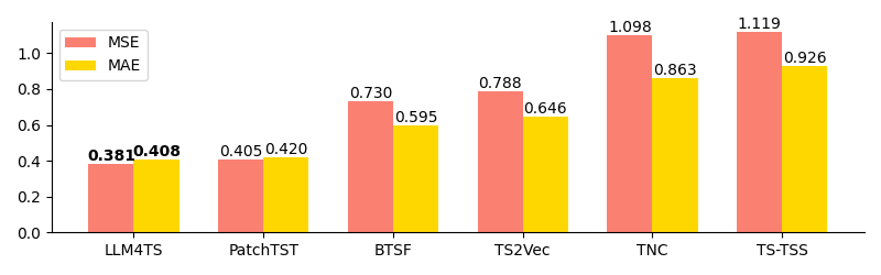
Figure 4: Self-supervised learning evaluation in forecasting with linear evaluation. We use results averaged over prediction lengths $T_{out}\in\{24,48,168,336,720\}$ for the ETTh1 dataset. The best average results are in bold. Details are reported in Appendix A.3.

5.2 Few-Shot Learning

Table 3 shows the results of using only $10\%$ and $5\%$ of the training data in long-term time-series forecasting. In our experiments, we maintain consistent splits for training, validation, and test sets in both full- and few-shot learning, and in few-shot scenarios, we intentionally limit the training data percentage. Both LLM4TS and GPT4TS Zhou et al. (2023) consistently surpass most train-from-scratch models in limited-data scenarios across various datasets, thanks to the pre-existing representation learning capability encapsulated in GPT-2. With the additional time-series alignment and multi-scale temporal information integration, LLM4TS emerges as a better data-efficient time-series forecaster against GPT4TS, achieving better performance across all datasets. Notably, LLM4TS with only $5\%$ of data outperforms the best baseline that uses $10\%$ of data.

5.3 Self-Supervised Learning

Given that the autoregressive objective used in the time-series alignment stage can be seen as a pretext task in self-supervised learning, we aim to assess LLM4TS’s representation learning capability. To evaluate the effectiveness of self-supervised learning, we conduct a linear evaluation on time-series forecasting. This involves pre-training the backbone model using the pretext task, freezing its weights, and then training an attached linear layer on the downstream forecasting task. With the backbone model’s parameters fixed, strong performance in forecasting depends on the expressiveness of the learned representations. Figure 4 shows LLM4TS’s superior performance over competitors on the ETTh1 dataset, highlighting the effectiveness of adapting the LLM to time-series characteristics in the time-series alignment stage.

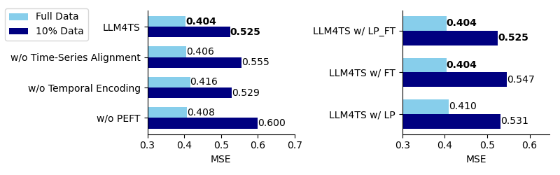
(a) Key Components in LLM4TS

(b) Training Strategies in Forecasting Fine-Tuning

Figure 5: Ablation study. Each ablation is conducted under both full- and few-shot learning with $10\%$ training data. We report results averaged over prediction lengths $T\in\{96,192,336,720\}$ for the ETTh1 dataset. The best average results are in bold. Details are reported in Appendix A.4.

5.4 Ablation Study

Key Components in LLM4TS

Figure 5(a) explores the effects of time-series alignment, temporal encoding, and PEFT in LLM4TS, assessing both full- and few-shot scenarios on the ETTh1 dataset. A comparative analysis—with and without these components—highlights their individual importance in enhancing forecasting accuracy in both scenarios. Notably, LLM4TS delivers exceptional performance in few-shot learning, averaging a $6.2\%$ reduction in MSE with each incorporation of these components.

Training Strategies in Forecasting Fine-Tuning

As discussed in Section 4.2, while full fine-tuning (FT) shows superior performance in out-of-distribution (OOD) scenarios and linear probing (LP) excels in in-distribution (ID) scenarios, LP-FT can surpass FT and LP in both OOD and ID scenarios. Figure 5(b) shows that LP-FT enhances performance in both full- and few-shot learning on the ETTh1 dataset, achieving an average improvement of $0.7\%$ in MSE for full-shot learning and $2.51\%$ for few-shot learning. The subtle improvements in both scenarios can be attributed to the limited number of trainable parameters in the LLM4TS’s backbone model even when using FT, which narrows the distinction between LP and FT. Notably, few-shot learning benefits more from LP-FT than full-shot learning, mainly because it is more susceptible to severe OOD issues.

6 Conclusion

In this paper, we present LLM4TS, a framework for time-series forecasting utilizing pre-trained LLMs. LLM4TS employs a two-stage fine-tuning strategy, beginning with the time-series alignment stage to adapt LLMs to the characteristics of time-series data, followed by the forecasting fine-tuning stage designed for time-series forecasting tasks. Our framework also introduces a novel two-level aggregation method, integrating multi-scale temporal data within pre-trained LLMs to improve their interpretation of time-related information. Through experiments on 7 time-series forecasting datasets, LLM4TS demonstrates superior performance over existing state-of-the-art methods, including those trained from scratch, in both full and few-shot scenarios.

In future work, we plan to extend our research in two directions. First, while we chose GPT-2 as our primary LLM in this paper for a fair comparison over GPT4TS, we plan to evaluate more recent LLMs like GPT-3.5 and LLaMA-2 to assess their advancements. Second, we aim to explore other tasks, such as classification and anomaly detection. Although forecasting is highly relevant to real-world applications without the need for manual labeling, extending it to other tasks enables the broader applicability of our LLM4TS framework.

Appendix A Detailed Results of Experiments

Table 4: Long-term forecasting for multivariate time-series data. We use prediction lengths $T\in\{96,192,336,720\}$ for all datasets. The best results are in bold, while the second-best results are underlined.

Methods		LLM4TS		GPT4TS		DLinear		PatchTST		FEDformer		Autoformer		Informer
Metric		MSE	MAE	MSE	MAE	MSE	MAE	MSE	MAE	MSE	MAE	MSE	MAE	MSE	MAE
Weather	96	0.147	0.196	0.162	0.212	0.176	0.237	0.149	0.198	0.217	0.296	0.266	0.336	0.300	0.384
	192	0.191	0.238	0.204	0.248	0.220	0.282	0.194	0.241	0.276	0.336	0.307	0.367	0.598	0.434
	336	0.241	0.277	0.254	0.286	0.265	0.319	0.245	0.282	0.339	0.380	0.359	0.395	0.578	0.523
	720	0.313	0.329	0.326	0.337	0.333	0.362	0.314	0.334	0.403	0.428	0.419	0.428	1.059	0.741
ETTh1	96	0.371	0.394	0.376	0.397	0.375	0.399	0.370	0.399	0.376	0.419	0.449	0.459	0.865	0.713
	192	0.403	0.412	0.416	0.418	0.405	0.416	0.413	0.421	0.420	0.448	0.500	0.482	1.008	0.792
	336	0.420	0.422	0.442	0.433	0.439	0.443	0.422	0.436	0.459	0.465	0.521	0.496	1.107	0.809
	720	0.422	0.444	0.477	0.456	0.472	0.490	0.447	0.466	0.506	0.507	0.514	0.512	1.181	0.865
ETTh2	96	0.269	0.332	0.285	0.342	0.289	0.353	0.274	0.336	0.358	0.397	0.346	0.388	3.755	1.525
	192	0.328	0.377	0.354	0.389	0.383	0.418	0.339	0.379	0.429	0.439	0.456	0.452	5.602	1.931
	336	0.353	0.396	0.373	0.407	0.448	0.465	0.329	0.380	0.496	0.487	0.482	0.486	4.721	1.835
	720	0.383	0.425	0.406	0.441	0.605	0.551	0.379	0.422	0.463	0.474	0.515	0.511	3.647	1.625
ETTm1	96	0.285	0.343	0.292	0.346	0.299	0.343	0.290	0.342	0.379	0.419	0.505	0.475	0.672	0.571
	192	0.324	0.366	0.332	0.372	0.335	0.365	0.332	0.369	0.426	0.441	0.553	0.496	0.795	0.669
	336	0.353	0.385	0.366	0.394	0.369	0.386	0.366	0.392	0.445	0.459	0.621	0.537	1.212	0.871
	720	0.408	0.419	0.417	0.421	0.425	0.421	0.416	0.420	0.543	0.490	0.671	0.561	1.166	0.823
ETTm2	96	0.165	0.254	0.173	0.262	0.167	0.269	0.165	0.255	0.203	0.287	0.255	0.339	0.365	0.453
	192	0.220	0.292	0.229	0.301	0.224	0.303	0.220	0.292	0.269	0.328	0.281	0.340	0.533	0.563
	336	0.268	0.326	0.286	0.341	0.281	0.342	0.274	0.329	0.325	0.366	0.339	0.372	1.363	0.887
	720	0.350	0.380	0.378	0.401	0.397	0.421	0.362	0.385	0.421	0.415	0.433	0.432	3.379	1.338
ECL	96	0.128	0.223	0.139	0.238	0.140	0.237	0.129	0.222	0.193	0.308	0.201	0.317	0.274	0.368
	192	0.146	0.240	0.153	0.251	0.153	0.249	0.157	0.240	0.201	0.315	0.222	0.334	0.296	0.386
	336	0.163	0.258	0.169	0.266	0.169	0.267	0.163	0.259	0.214	0.329	0.231	0.338	0.300	0.394
	720	0.200	0.292	0.206	0.297	0.203	0.301	0.197	0.290	0.246	0.355	0.254	0.361	0.373	0.439
Traffic	96	0.372	0.259	0.388	0.282	0.410	0.282	0.360	0.249	0.587	0.366	0.613	0.388	0.719	0.391
	192	0.391	0.265	0.407	0.290	0.423	0.287	0.379	0.256	0.604	0.373	0.616	0.382	0.696	0.379
	336	0.405	0.275	0.412	0.294	0.436	0.296	0.392	0.264	0.621	0.383	0.622	0.337	0.777	0.420
	720	0.437	0.292	0.450	0.312	0.466	0.315	0.432	0.286	0.626	0.382	0.660	0.408	0.864	0.472

We include detailed tables for the entire set of experiments in the appendices: long-term forecasting (Appendix A.1), few-shot learning (Appendix A.2), self-supervised learning (Appendix A.3), and ablation studies (Appendix A.4). All results for various prediction lengths are provided in these tables

A.1 Long-term Time-Series Forecasting

Table 4 showcases the outcomes of long-term time-series forecasting, maintaining a consistent prediction length set $T_{out}\in\{96,192,336,720\}$ across all datasets. While the primary focus of using pre-trained LLMs is on few-shot learning, LLM4TS notably outperforms all deep train-from-scratch methods, even with full dataset access. Its two-stage fine-tuning approach and integration of multi-scale temporal information enable LLM4TS to secure the top rank in 9 out of 14 evaluations, spanning 7 datasets and 2 metrics. Interestingly, for the largest dataset (Traffic), PatchTST emerges as the leading model. This suggests that with complete dataset access and sufficient data volume, traditional deep train-from-scratch models may sometimes outshine those leveraging pre-trained LLMs.

Table 5: Few-shot long-term forecasting using $10\%$ of the training data. We use prediction lengths $T\in\{96,192,336,720\}$ for all datasets. The best results are in bold, while the second-best results are underlined.

Methods		LLM4TS		GPT4TS		DLinear		PatchTST		FEDformer		Autoformer		Informer
Metric		MSE	MAE	MSE	MAE	MSE	MAE	MSE	MAE	MSE	MAE	MSE	MAE	MSE	MAE
Weather	96	0.158	0.207	0.163	0.215	0.171	0.224	0.165	0.215	0.188	0.253	0.221	0.297	0.374	0.401
	192	0.204	0.249	0.210	0.254	0.215	0.263	0.210	0.257	0.250	0.304	0.270	0.322	0.552	0.478
	336	0.254	0.288	0.256	0.292	0.258	0.299	0.259	0.297	0.312	0.346	0.320	0.351	0.724	0.541
	720	0.322	0.336	0.321	0.339	0.320	0.346	0.332	0.346	0.387	0.393	0.390	0.396	0.739	0.558
ETTh1	96	0.417	0.432	0.458	0.456	0.492	0.495	0.516	0.485	0.512	0.499	0.613	0.552	1.179	0.792
	192	0.469	0.468	0.570	0.516	0.565	0.538	0.598	0.524	0.624	0.555	0.722	0.598	1.199	0.806
	336	0.505	0.499	0.608	0.535	0.721	0.622	0.657	0.550	0.691	0.574	0.750	0.619	1.202	0.811
	720	0.708	0.572	0.725	0.591	0.986	0.743	0.762	0.610	0.728	0.614	0.721	0.616	1.217	0.825
ETTh2	96	0.282	0.351	0.331	0.374	0.357	0.411	0.353	0.389	0.382	0.416	0.413	0.451	3.837	1.508
	192	0.364	0.400	0.402	0.411	0.569	0.519	0.403	0.414	0.478	0.474	0.474	0.477	3.856	1.513
	336	0.374	0.416	0.406	0.433	0.671	0.572	0.426	0.441	0.504	0.501	0.547	0.543	3.952	1.526
	720	0.445	0.461	0.449	0.464	0.824	0.648	0.477	0.480	0.499	0.509	0.516	0.523	3.842	1.503
ETTm1	96	0.360	0.388	0.390	0.404	0.352	0.392	0.410	0.419	0.578	0.518	0.774	0.614	1.162	0.785
	192	0.386	0.401	0.429	0.423	0.382	0.412	0.437	0.434	0.617	0.546	0.754	0.592	1.172	0.793
	336	0.415	0.417	0.469	0.439	0.419	0.434	0.476	0.454	0.998	0.775	0.869	0.677	1.227	0.908
	720	0.470	0.445	0.569	0.498	0.490	0.477	0.681	0.556	0.693	0.579	0.810	0.630	1.207	0.797
ETTm2	96	0.184	0.265	0.188	0.269	0.213	0.303	0.191	0.274	0.291	0.399	0.352	0.454	3.203	1.407
	192	0.240	0.301	0.251	0.309	0.278	0.345	0.252	0.317	0.307	0.379	0.694	0.691	3.112	1.387
	336	0.294	0.337	0.307	0.346	0.338	0.385	0.306	0.353	0.543	0.559	2.408	1.407	3.255	1.421
	720	0.386	0.393	0.426	0.417	0.436	0.440	0.433	0.427	0.712	0.614	1.913	1.166	3.909	1.543
ECL	96	0.135	0.231	0.139	0.237	0.150	0.253	0.140	0.238	0.231	0.323	0.261	0.348	1.259	0.919
	192	0.152	0.246	0.156	0.252	0.164	0.264	0.160	0.255	0.261	0.356	0.338	0.406	1.160	0.873
	336	0.173	0.267	0.175	0.270	0.181	0.282	0.180	0.276	0.360	0.445	0.410	0.474	1.157	0.872
	720	0.229	0.312	0.233	0.317	0.223	0.321	0.241	0.323	0.530	0.585	0.715	0.685	1.203	0.898
Traffic	96	0.402	0.288	0.414	0.297	0.419	0.298	0.403	0.289	0.639	0.400	0.672	0.405	1.557	0.821
	192	0.416	0.294	0.426	0.301	0.434	0.305	0.415	0.296	0.637	0.416	0.727	0.424	1.454	0.765
	336	0.429	0.302	0.434	0.303	0.449	0.313	0.426	0.304	0.655	0.427	0.749	0.454	1.521	0.812
	720	0.480	0.326	0.487	0.337	0.484	0.336	0.474	0.331	0.722	0.456	0.847	0.499	1.605	0.846

Table 6: Few-shot long-term forecasting using $5\%$ of the training data. For most datasets, results are reported over prediction lengths $T_{out}\in\{96,192,336,720\}$. However, for datasets marked with * (ETTh1, ETTh2, and Traffic), only $T_{out}\in\{96,192,336\}$ are used because there are insufficient data to constitute a training set when $T_{out}=720$. The best results are in bold, while the second-best results are in underlined.

Methods		LLM4TS		GPT4TS		DLinear		PatchTST		FEDformer		Autoformer		Informer
Metric		MSE	MAE	MSE	MAE	MSE	MAE	MSE	MAE	MSE	MAE	MSE	MAE	MSE	MAE
Weather	96	0.173	0.227	0.175	0.230	0.184	0.242	0.171	0.224	0.229	0.309	0.227	0.299	0.497	0.497
	192	0.218	0.265	0.227	0.276	0.228	0.283	0.230	0.277	0.265	0.317	0.278	0.333	0.620	0.545
	336	0.276	0.310	0.286	0.322	0.279	0.322	0.294	0.326	0.353	0.392	0.351	0.393	0.649	0.547
	720	0.355	0.366	0.366	0.379	0.364	0.388	0.384	0.387	0.391	0.394	0.387	0.389	0.570	0.522
ETTh1*	96	0.509	0.484	0.543	0.506	0.547	0.503	0.557	0.519	0.593	0.529	0.681	0.570	1.225	0.812
	192	0.717	0.581	0.748	0.580	0.720	0.604	0.711	0.570	0.652	0.563	0.725	0.602	1.249	0.828
	336	0.728	0.589	0.754	0.595	0.984	0.727	0.816	0.619	0.731	0.594	0.761	0.624	1.202	0.811
	720	-	-	-	-	-	-	-	-	-	-	-	-	-	-
ETTh2*	96	0.314	0.375	0.376	0.421	0.442	0.456	0.401	0.421	0.390	0.424	0.428	0.468	3.837	1.508
	192	0.365	0.408	0.418	0.441	0.617	0.542	0.452	0.455	0.457	0.465	0.496	0.504	3.975	1.933
	336	0.398	0.432	0.408	0.439	1.424	0.849	0.464	0.469	0.477	0.483	0.486	0.496	3.956	1.520
	720	-	-	-	-	-	-	-	-	-	-	-	-	-	-
ETTm1	96	0.349	0.379	0.386	0.405	0.332	0.374	0.399	0.414	0.628	0.544	0.726	0.578	1.130	0.775
	192	0.374	0.394	0.440	0.438	0.358	0.390	0.441	0.436	0.666	0.566	0.750	0.591	1.150	0.788
	336	0.411	0.417	0.485	0.459	0.402	0.416	0.499	0.467	0.807	0.628	0.851	0.659	1.198	0.809
	720	0.516	0.479	0.577	0.499	0.511	0.489	0.767	0.587	0.822	0.633	0.857	0.655	1.175	0.794
ETTm2	96	0.192	0.273	0.199	0.280	0.236	0.326	0.206	0.288	0.229	0.320	0.232	0.322	3.599	1.478
	192	0.249	0.309	0.256	0.316	0.306	0.373	0.264	0.324	0.394	0.361	0.291	0.357	3.578	1.475
	336	0.301	0.342	0.318	0.353	0.380	0.423	0.334	0.367	0.378	0.427	0.478	0.517	3.561	1.473
	720	0.402	0.405	0.460	0.436	0.674	0.583	0.454	0.432	0.523	0.510	0.553	0.538	3.896	1.533
ECL	96	0.139	0.235	0.143	0.241	0.150	0.251	0.145	0.244	0.235	0.322	0.297	0.367	1.265	0.919
	192	0.155	0.249	0.159	0.255	0.163	0.263	0.163	0.260	0.247	0.341	0.308	0.375	1.298	0.939
	336	0.174	0.269	0.179	0.274	0.175	0.278	0.183	0.281	0.267	0.356	0.354	0.411	1.302	0.942
	720	0.222	0.310	0.233	0.323	0.219	0.311	0.233	0.323	0.318	0.394	0.426	0.466	1.259	0.919
Traffic*	96	0.401	0.285	0.419	0.298	0.427	0.304	0.404	0.286	0.670	0.421	0.795	0.481	1.557	0.821
	192	0.418	0.293	0.434	0.305	0.447	0.315	0.412	0.294	0.653	0.405	0.837	0.503	1.596	0.834
	336	0.436	0.308	0.449	0.313	0.478	0.333	0.439	0.310	0.707	0.445	0.867	0.523	1.621	0.841
	720	-	-	-	-	-	-	-	-	-	-	-	-	-	-

A.2 Few-Shot Learning

Table 5 shows the results of long-term time-series forecasting using only $10\%$ of the training data, while Table 6 presents similar results but with merely $5\%$ of the training data utilized. In our experiments, consistent splits for training, validation, and test sets are maintained across both full and few-shot learning scenarios. We deliberately limited the training data percentage to 10% and 5% to evaluate model performance in few-shot scenarios. LLM4TS and GPT4TS Zhou et al. [2023] consistently outperformed most deep train-from-scratch models in these limited-data scenarios across various datasets, a success attributed to the inherent representation learning capabilities of GPT-2. Enhanced by additional time-series alignment and multi-scale temporal information integration, LLM4TS proves to be a better data-efficient time-series forecaster compared to GPT4TS, delivering superior performance across all datasets. Remarkably, with only $5\%$ of data, LLM4TS surpasses the top baseline using $10\%$ of data.

For the largest dataset (Traffic), PatchTST emerges as the leading model in the full-shot scenario, though this trend does not extend to few-shot scenarios. With only $10\%$ training data, LLM4TS outperforms PatchTST in 5 out of 8 evaluations, and with just $5\%$ training data, it leads in 5 out of 6 evaluations. This suggests that in few-shot scenarios, traditional deep train-from-scratch models generally still underperform compared to those leveraging pre-trained LLMs.

Table 7: Self-supervised learning evaluation in forecasting with linear probing. We use prediction lengths $T_{out}\in\{24,48,168,336,720\}$ for the ETTh1 dataset. The best average results are in bold, while the second-best results are in underlined.

Methods		LLM4TS		PatchTST		BTSF		TS2Vec		TNC		TS-TCC
Metric		MSE	MAE	MSE	MAE	MSE	MAE	MSE	MAE	MSE	MAE	MSE	MAE
ETTh1	24	0.315	0.365	0.322	0.369	0.541	0.519	0.599	0.534	0.632	0.596	0.653	0.61
	48	0.342	0.384	0.354	0.385	0.613	0.524	0.629	0.555	0.705	0.688	0.72	0.693
	168	0.401	0.415	0.419	0.424	0.64	0.532	0.755	0.636	1.097	0.993	1.129	1.044
	336	0.421	0.427	0.445	0.446	0.864	0.689	0.907	0.717	1.454	0.919	1.492	1.076
	720	0.426	0.447	0.487	0.478	0.993	0.712	1.048	0.79	1.604	1.118	1.603	1.206
	Avg.	0.381	0.408	0.405	0.420	0.730	0.595	0.788	0.646	1.098	0.863	1.119	0.926

A.3 Self-Supervised Learning

Table 7 showcases LLM4TS’s outstanding performance on the ETTh1 dataset, underscoring the success of adapting the LLM to time-series characteristics during the time-series alignment stage. This comparison exclusively includes self-supervised learning methods, thereby excluding deep train-from-scratch models designed explicitly for time-series forecasting. Similarly, GPT4TS is not part of this experiment as it lacks a distinct stage of representation learning. The variant of PatchTST used here differs from that in the forecasting experiments; this variant focuses on representation learning. PatchTST incorporates an MLM (Masked Language Model) approach, akin to BERT, for learning representations. Despite this, LLM4TS still emerges as the top method in representation learning capability among all evaluated methods, achieving an average improvement of $6.02\%$ in MSE.

Table 8: Ablation study. Each ablation is conducted under standard and few-shot learning with 10% training data. IMP. denotes the average improvement achieved by incorporating one of LLM4TS’s core components. We use prediction lengths $T_{out}\in\{96,192,336,720\}$ for the ETTh1 dataset. The best average results are in bold.

(a) Ablation study of time-series alignment, temporal encoding, and PEFT in LLM4TS.

Methods		IMP.	LLM4TS		w/o Time-Series Fine-Tuning		w/o Temporal Encoding		w/o PEFT
Metric		MSE	MSE	MAE	MSE	MAE	MSE	MAE	MSE	MAE
ETTh1 (full)	96	0.89%	0.371	0.394	0.372	0.395	0.378	0.397	0.373	0.393
	192	1.14%	0.403	0.412	0.404	0.411	0.411	0.416	0.408	0.412
	336	1.16%	0.42	0.422	0.422	0.423	0.433	0.43	0.42	0.421
	720	2.21%	0.422	0.444	0.424	0.448	0.442	0.457	0.429	0.45
	Avg.	1.37%	0.404	0.418	0.406	0.419	0.416	0.425	0.408	0.419
ETTh1 (10%)	96	1.80%	0.417	0.432	0.43	0.438	0.422	0.434	0.422	0.433
	192	1.01%	0.469	0.468	0.488	0.474	0.463	0.465	0.471	0.462
	336	4.03%	0.505	0.499	0.538	0.506	0.516	0.508	0.525	0.504
	720	11.89%	0.708	0.572	0.762	0.589	0.714	0.584	0.98	0.672
	Avg.	6.20%	0.525	0.493	0.555	0.502	0.529	0.498	0.600	0.518

(b) Ablation study of training strategies during forecasting fine-tuning.

Methods		IMP.	LLM4TS w/ LP_FT (Ours)		LLM4TS w/ FT		LLM4TS w/ LP
Metric		MSE	MSE	MAE	MSE	MAE	MSE	MAE
ETTh1 (full)	96	0.80%	0.371	0.394	0.371	0.394	0.377	0.398
	192	0.98%	0.403	0.412	0.404	0.413	0.41	0.416
	336	0.70%	0.42	0.422	0.42	0.423	0.426	0.424
	720	0.35%	0.422	0.444	0.42	0.444	0.427	0.447
	Avg.	0.70%	0.404	0.418	0.404	0.419	0.410	0.421
ETTh1 (10%)	96	0.12%	0.421	0.435	0.423	0.436	0.42	0.433
	192	2.52%	0.454	0.457	0.477	0.474	0.455	0.454
	336	2.36%	0.515	0.504	0.545	0.524	0.511	0.507
	720	3.92%	0.711	0.574	0.743	0.589	0.737	0.589
	Avg.	2.51%	0.525	0.493	0.547	0.506	0.531	0.496

A.4 Ablation Study

Key Components in LLM4TS

Table 8(a) explores the effects of time-series alignment, temporal encoding, and PEFT in LLM4TS, assessing both full- and few-shot scenarios on the ETTh1 dataset. A comparative analysis—with and without these components—highlights their individual importance in enhancing forecasting accuracy in both scenarios. Notably, LLM4TS delivers exceptional performance in few-shot learning, averaging a $6.2\%$ reduction in MSE with each incorporation of these components. We can observe two things in the experimental results. The first one is the MSE improvement is increasing when the prediction length is also increasing. This indicate that the main components have greater benefits when the requirement of the model’s prediction capability is increased. The second one is the few-shot scenarios benefit more than full-shot scenarios when we incorporate these main components in LLM4TS. This indicates that the model benefits more than the incorporation of the LLM4TS’s compoments when the volumn of training data is limited. This proves that LLM4TS is an excellent data-efficient time-series forecaster since the main components of its own.

In the experimental results, we observe two key insights. First, there is a notable trend where the MSE improvement increases as the prediction length extends. This indicates that the core elements of LLM4TS become increasingly beneficial in situations where a higher level of predictive capability is required, particularly evident with longer prediction lengths. Second, few-shot scenarios exhibit more substantial gains than full-shot scenarios upon integrating these main components into LLM4TS. It emphasizes LLM4TS’s strength as a data-efficient time-series forecaster, a quality primarily attributed to its intrinsic components.

Training Strategies in Forecasting Fine-Tuning

Table 8(b) demonstrates that LP-FT boosts performance on the ETTh1 dataset in both full- and few-shot learning scenarios, with an average MSE improvement of $0.7\%$ in full-shot and $2.51\%$ in few-shot learning. The subtle enhancements in both cases are likely due to the limited number of trainable parameters in LLM4TS’s backbone model even with FT, leading to a more negligible differentiation between LP and FT. The results further reveal that few-shot learning derives a greater advantage from LP-FT, primarily due to its higher vulnerability to severe OOD issues. Additionally, consistent with observations in the ablation study of LLM4TS’s main components, we note a similar trend where longer prediction lengths yield more significant benefits in few-shot scenarios.

References

- Chang et al. [2023] Ching Chang, Chiao-Tung Chan, Wei-Yao Wang, Wen-Chih Peng, and Tien-Fu Chen. Timedrl: Disentangled representation learning for multivariate time-series. arXiv preprint arXiv:2312.04142, 2023.
- Eldele et al. [2021] Emadeldeen Eldele, Mohamed Ragab, Zhenghua Chen, Min Wu, C. Kwoh, Xiaoli Li, and Cuntai Guan. Time-series representation learning via temporal and contextual contrasting. In International Joint Conference on Artificial Intelligence, 2021.
- Ghosal et al. [2023] Deepanway Ghosal, Navonil Majumder, Ambuj Mehrish, and Soujanya Poria. Text-to-audio generation using instruction-tuned llm and latent diffusion model. ArXiv, abs/2304.13731, 2023.
- Giannou et al. [2023] Angeliki Giannou, Shashank Rajput, Jy-yong Sohn, Kangwook Lee, Jason D Lee, and Dimitris Papailiopoulos. Looped transformers as programmable computers. arXiv preprint arXiv:2301.13196, 2023.
- Hegselmann et al. [2023] Stefan Hegselmann, Alejandro Buendia, Hunter Lang, Monica Agrawal, Xiaoyi Jiang, and David Sontag. Tabllm: Few-shot classification of tabular data with large language models. In International Conference on Artificial Intelligence and Statistics, pages 5549–5581. PMLR, 2023.
- Hoffmann et al. [2022] Jordan Hoffmann, Sebastian Borgeaud, Arthur Mensch, Elena Buchatskaya, Trevor Cai, Eliza Rutherford, Diego de Las Casas, Lisa Anne Hendricks, Johannes Welbl, Aidan Clark, et al. Training compute-optimal large language models. arXiv preprint arXiv:2203.15556, 2022.
- Hu et al. [2021] Edward J Hu, Yelong Shen, Phillip Wallis, Zeyuan Allen-Zhu, Yuanzhi Li, Shean Wang, Lu Wang, and Weizhu Chen. Lora: Low-rank adaptation of large language models. arXiv preprint arXiv:2106.09685, 2021.
- Kim et al. [2021] Taesung Kim, Jinhee Kim, Yunwon Tae, Cheonbok Park, Jang-Ho Choi, and Jaegul Choo. Reversible instance normalization for accurate time-series forecasting against distribution shift. In International Conference on Learning Representations, 2021.
- Kumar et al. [2022] Ananya Kumar, Aditi Raghunathan, Robbie Jones, Tengyu Ma, and Percy Liang. Fine-tuning can distort pretrained features and underperform out-of-distribution. arXiv preprint arXiv:2202.10054, 2022.
- Lai et al. [2018] Guokun Lai, Wei-Cheng Chang, Yiming Yang, and Hanxiao Liu. Modeling long-and short-term temporal patterns with deep neural networks. In The 41st international ACM SIGIR conference on research & development in information retrieval, pages 95–104, 2018.
- Liu et al. [2021] Minghao Liu, Shengqi Ren, Siyuan Ma, Jiahui Jiao, Yizhou Chen, Zhiguang Wang, and Wei Song. Gated transformer networks for multivariate time series classification. arXiv preprint arXiv:2103.14438, 2021.
- Lu et al. [2021] Kevin Lu, Aditya Grover, Pieter Abbeel, and Igor Mordatch. Pretrained transformers as universal computation engines. arXiv preprint arXiv:2103.05247, 1, 2021.
- Nie et al. [2023] Yuqi Nie, Nam H. Nguyen, Phanwadee Sinthong, and Jayant Kalagnanam. A time series is worth 64 words: Long-term forecasting with transformers. In ICLR. OpenReview.net, 2023.
- Radford et al. [2019] Alec Radford, Jeffrey Wu, Rewon Child, David Luan, Dario Amodei, Ilya Sutskever, et al. Language models are unsupervised multitask learners. OpenAI blog, 1:9, 2019.
- Tonekaboni et al. [2021] Sana Tonekaboni, Danny Eytan, and Anna Goldenberg. Unsupervised representation learning for time series with temporal neighborhood coding. In ICLR. OpenReview.net, 2021.
- Touvron et al. [2023] Hugo Touvron, Thibaut Lavril, Gautier Izacard, Xavier Martinet, Marie-Anne Lachaux, Timothée Lacroix, Baptiste Rozière, Naman Goyal, Eric Hambro, Faisal Azhar, Aurelien Rodriguez, Armand Joulin, Edouard Grave, and Guillaume Lample. Llama: Open and efficient foundation language models. ArXiv, abs/2302.13971, 2023.
- Wu et al. [2021] Haixu Wu, Jiehui Xu, Jianmin Wang, and Mingsheng Long. Autoformer: Decomposition transformers with auto-correlation for long-term series forecasting. Advances in Neural Information Processing Systems, 34:22419–22430, 2021.
- Xu et al. [2021] Jiehui Xu, Haixu Wu, Jianmin Wang, and Mingsheng Long. Anomaly transformer: Time series anomaly detection with association discrepancy. arXiv preprint arXiv:2110.02642, 2021.
- Yang and Hong [2022] Ling Yang and Shenda Hong. Unsupervised time-series representation learning with iterative bilinear temporal-spectral fusion. In International Conference on Machine Learning, pages 25038–25054. PMLR, 2022.
- Yeh et al. [2019] Cheng-Han Yeh, Yao-Chung Fan, and Wen-Chih Peng. Interpretable multi-task learning for product quality prediction with attention mechanism. In 2019 IEEE 35th International Conference on Data Engineering (ICDE), pages 1910–1921. IEEE, 2019.
- Yue et al. [2022] Zhihan Yue, Yujing Wang, Juanyong Duan, Tianmeng Yang, Congrui Huang, Yunhai Tong, and Bixiong Xu. Ts2vec: Towards universal representation of time series. In Proceedings of the AAAI Conference on Artificial Intelligence, volume 36, pages 8980–8987, 2022.
- Zeng et al. [2023] Ailing Zeng, Muxi Chen, Lei Zhang, and Qiang Xu. Are transformers effective for time series forecasting? In Proceedings of the AAAI conference on artificial intelligence, volume 37, pages 11121–11128, 2023.
- Zhang et al. [2022] Xiang Zhang, Ziyuan Zhao, Theodoros Tsiligkaridis, and Marinka Zitnik. Self-supervised contrastive pre-training for time series via time-frequency consistency. Advances in Neural Information Processing Systems, 35:3988–4003, 2022.
- Zhou et al. [2021] Haoyi Zhou, Shanghang Zhang, Jieqi Peng, Shuai Zhang, Jianxin Li, Hui Xiong, and Wancai Zhang. Informer: Beyond efficient transformer for long sequence time-series forecasting. In Proceedings of the AAAI conference on artificial intelligence, volume 35, pages 11106–11115, 2021.
- Zhou et al. [2022] Tian Zhou, Ziqing Ma, Qingsong Wen, Xue Wang, Liang Sun, and Rong Jin. Fedformer: Frequency enhanced decomposed transformer for long-term series forecasting. In International Conference on Machine Learning, pages 27268–27286. PMLR, 2022.
- Zhou et al. [2023] Tian Zhou, Peisong Niu, Xue Wang, Liang Sun, and Rong Jin. One fits all: Power general time series analysis by pretrained lm. arXiv preprint arXiv:2302.11939, 2023.