Hierarchical Uncertainty Estimation for
Medical Image Segmentation Networks

Abstract

Learning a medical image segmentation model is an inherently ambiguous task, as uncertainties exist in both images (noise) and manual annotations (human errors and bias) used for model training. To build a trustworthy image segmentation model, it is important to not just evaluate its performance but also estimate the uncertainty of the model prediction. Most state-of-the-art image segmentation networks adopt a hierarchical encoder architecture, extracting image features at multiple resolution levels from fine to coarse. In this work, we leverage this hierarchical image representation and propose a simple yet effective method for estimating uncertainties at multiple levels. The multi-level uncertainties are modelled via the skip-connection module and then sampled to generate an uncertainty map for the predicted image segmentation. We demonstrate that a deep learning segmentation network such as U-net, when implemented with such hierarchical uncertainty estimation module, can achieve a high segmentation performance, while at the same time provide meaningful uncertainty maps that can be used for out-of-distribution detection. The code is publicly available here.

1 Introduction

Image segmentation plays an essential role in medical image analysis, which enables extraction of clinically relevant information about anatomical structures, detection of abnormalities and visualisation of regions of interest. In recent years, automated medical image segmentation has made solid progress with deep learning. Given clinicians’ concerns over exclusive reliance on automated segmentations for critical decisions [5], one of the solutions is to corporate uncertainty estimation into the network. This not only improves model interpretability for ambiguous areas, but also serves as a safeguard for unexpected inputs.

In this work, we propose a generic hierarchical uncertainty estimation framework, named as VAE U-net, for medical image segmentation task. VAE U-net integrates uncertainty modelling with the skip-connection module between encoder and decoder. Different from previous works [4, 15], the sampled latent features are directly fed into the decoder without upsampling and then concatenated with features from the skip-connection layer. This may allow the gradients to flow easily to the initial layers of the encoder to learn good representations. We demonstrate that VAE U-net achieves state-of-the-art segmentation performance while captures a very good estimation of the uncertainty as a light-weight model.

2 Related Works

Capturing uncertainty within the learning process is often implemented by model ensemble or by using variational Bayesian methods [2]. For model ensembling, Lakshminarayanan et al. [16] introduced a randomisation-based approach to ensemble multiple networks and showed that majority voting using these networks greatly improves the accuracy. A more advanced technique to produce diversified weight samples was proposed in [21], which includes cyclical learning rate and multi-modal checkpoint ensemble. Limitations for model ensemble include reduced interpretability as well as additional costs in computation time.

Apart from model ensemble, variational inference provides another way for estimating uncertainty [10]. Dropout [19], initially proposed as a regularization layer, is recognised as a way for approximate inference in a complex network [8]. Similar techniques were adopted by flipout [20], which perturbs the weight distribution in mini-batches. More recent works are dedicated to introducing auxiliary modules to an existing network. To directly learn the uncertainty from samples, Kohl et al. [13] included a side branch to the U-net architecture to learn the latent distribution with a conditional variational auto-encoder. Later, architectures that used hierarchical probabilistic U-net to model ambiguities at multiple scales were proposed [4, 15], where the uncertainty estimator was interleaved with feature extraction by the decoder.

3 Methods

3.1 Problem Formulation

Let $X$ denote the input image and $Y$ denote the segmentation map. The image $X$ is mapped to a latent space $z$ via an encoder $q_{\phi}(\mathbf{z}\mid X)$, which describes the posterior distribution of $z$ conditioned on $X$. In a variational auto-encoder (VAE), the posterior $q_{\phi}(\mathbf{z}\mid X)$ is typically constrained by a prior $p(z)$ which is a Gaussian distribution. We assume that the segmentation $Y$ can be mapped to the same latent space $z$ via an encoder $p_{\theta}(\mathbf{z}\mid Y)$, i.e. the image and the segmentation share an aligned latent space. Based on this assumption, we formulate the following learning objective,

$$\max_{\theta,\phi}\mathbb{E}_{X,Y\sim D}[\mathbb{E}_{z\sim q_{\phi}(\mathbf{z}\mid X)}[\log p_{\theta}(Y\mid\mathbf{z})]]$$ (1)

$$\textrm{subj. to}\quad D_{KL}[q_{\phi}(\mathbf{z}\mid X)||p_{\theta}(\mathbf{z}\mid Y)]<\epsilon$$ (2)

Here $D$ denotes the dataset of both images $X$ and segmentations $Y$, the objective function aims to maximise the probability of the observed segmentation $Y$ given the latent space distribution $q_{\phi}(\mathbf{z}\mid X)$. A Kullback-Leibler (KL) divergence $D_{KL}$ is introduced to match the distribution $q_{\phi}(\mathbf{z}\mid X)$ and $p_{\theta}(\mathbf{z}\mid Y)$.

Inspired by $\beta$-VAE [11] and rewriting the optimisation problem using the Lagrangian multiplier $\beta$, we have,

$$\mathcal{F}(\theta,\phi,\beta;Y,\mathbf{z}) =\mathbb{E}_{q_{\phi}(\mathbf{z}\mid X)}[\log p_{\theta}(Y\mid\mathbf{z})]-\beta(D_{KL}[q_{\phi}(\mathbf{z}\mid X)||p_{\theta}(\mathbf{z}\mid Y)]-\epsilon)$$ (3)

$$\geq\mathbb{E}_{q_{\phi}(\mathbf{z}\mid X)}[\log p_{\theta}(Y\mid\mathbf{z})]-\beta D_{KL}[q_{\phi}(\mathbf{z}\mid X)||p_{\theta}(\mathbf{z}\mid Y)]$$ (4)

We aim to maximise the lower bound of the objective function,

$$\mathcal{L}=\mathbb{E}_{q_{\phi}(\mathbf{z}\mid X)}[\log p_{\theta}(Y\mid\mathbf{z})]-\beta D_{KL}[q_{\phi}(\mathbf{z}\mid X)||p_{\theta}(\mathbf{z}\mid Y)]$$ (5)

In this work, we employ the binary cross entropy loss for the first term, which evaluates the reconstruction accuracy for the predicted segmentation, compared to ground truth. $\beta$ denotes a regularization weight, which encourages the posterior $q_{\phi}$ to be close to the prior $p_{\theta}$.

3.2 Hierarchical Representation

Without loss of generality, we assume a multi-level network such as U-net is used for the segmentation task, which contains skip connections at multiple resolution levels. These skip connections encode rich image features, which allow us to model the data uncertainties at different resolution levels. Given a U-net of $L+1$ resolution levels, we introduce a number of latent variables $z_{i}(i=0,\dots,L)$ to describe the latent representation at resolution level $i$. These latents are inferred from the feature maps at the skip connections. They are inter-dependent as fine resolution features are normally built upon coarse resolution features. For instance, $z_{0}$ denotes the latent variable from the top level skip connection features extracted directly from the input image. $z_{1}$ denotes the latent variable from the second level, which has a dependency on $z_{0}$. Therefore, the image-to-latent encoder $q_{\phi}$ and segmentation-to-latent encoder $p_{\theta}$ can be expanded with the product rule:

$$q_{\phi}(\mathbf{z}\mid X) =q_{\phi}(z_{L}\mid z_{<L},X)\cdot...\cdot q_{\phi}(z_{0}\mid X)$$ (6)

$$p_{\theta}(\mathbf{z}\mid Y) =p_{\theta}(z_{L}\mid z_{<L},Y)\cdot...\cdot p_{\theta}(z_{0}\mid Y)$$ (7)

The KL-divergence between the two distribution can be expanded hierarchically [14] as,

$$\quad D_{KL}[q_{\phi}(\mathbf{z}\mid X)||p_{\theta}(\mathbf{z}\mid Y)]$$ (8)

$$=\mathbb{E}_{z\sim q_{\phi}(\mathbf{z}\mid X)}[\log q_{\phi}(\mathbf{z}\mid X)-\log p_{\theta}(\mathbf{z}\mid Y)]$$ (9)

$$=\int_{\mathbf{z}}\Pi^{L}_{j=0}q_{\phi}(z_{j}\mid z_{<j},X)\sum^{L}_{i=0}[\log q_{\phi}(z_{i}\mid z_{<i},X)-\log p_{\theta}(z_{i}\mid z_{<i},Y)]dz_{0}...dz_{L}$$ (10)

$$=\sum^{L}_{i=0}\int_{\mathbf{z}}\Pi^{i}_{j=0}q_{\phi}(z_{j}\mid z_{<j},X)[\log q_{\phi}(z_{i}\mid z_{<i},X)-\log p_{\theta}(z_{i}\mid z_{<i},Y)]dz_{0}...dz_{L}$$ (11)

$$=\sum^{L}_{i=0}\int_{\mathbf{z}}\Pi^{i-1}_{j=0}q_{\phi}(z_{j}\mid z_{<j},X)q_{\phi}(z_{i}\mid z_{<i},X)[\log q_{\phi}(z_{i}\mid z_{<i},X)$$ (12)

$$\qquad-\log p_{\theta}(z_{i}\mid z_{<i},Y)]dz_{0}...dz_{L}$$ (13)

$$=\sum^{L}_{i=0}\mathbb{E}_{\mathbf{z}_{<i}\sim q_{\phi}(\mathbf{z}\mid X)}[D_{KL}[q_{\phi}(z_{i}\mid z_{<i},X)||p_{\theta}(z_{i}\mid z_{<i},Y)]]$$ (14)

This means that the KL-divergence term can be evaluated separately for each resolution level, which eases the implementation. Note that for simplicity, $p_{\theta}(z_{0}\mid z_{<0})$ and $q_{\phi}(z_{0}\mid z_{<0})$ represents for $p_{\theta}(z_{0})$ and $q_{\phi}(z_{0})$ separately. Plugging this formulation into the KL-divergence in Eq. (14), we have the following objective function,

$$\mathcal{L}=\mathbb{E}_{q_{\phi}(\mathbf{z}\mid X)}[\log p_{\theta}(Y\mid\mathbf{z})]-\beta\sum^{L}_{i=0}\mathbb{E}_{\mathbf{z}_{<i}\sim q_{\phi}(\mathbf{z}\mid X)}[D_{KL}[q_{\phi}(z_{i}\mid z_{<i},X)||p_{\theta}(z_{i}\mid z_{<i},Y)]]$$ (15)

The expectation of the first term can be performed with a single pass Monte-Carlo sampling [12] in the implementation.

3.3 Proposed Architecture

Figure 1 illustrates the overall structure of the proposed segmentation framework with uncertainty awareness, named as VAE U-net.

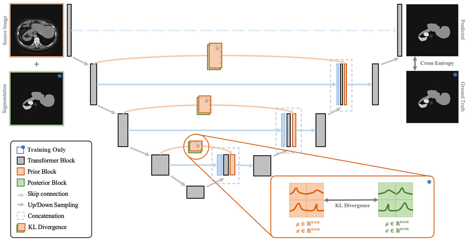
Figure 1: Hierarchical uncertainty estimation architecture. The structure of the network is based on U-net, with VAE modules that accompany the skip connections to model the uncertainty at multiple resolution levels.

The network follows the typical setup of a U-net architecture, composed of encoder and decoder modules. At the training stage, it takes both the image $X$ and the segmentation $Y$, aiming to generate the correct segmentation while at the meantime matching the latent distributions $q_{\phi}(\mathbf{z}\mid X)$ and $p_{\theta}(\mathbf{z}\mid Y)$. The latents are modelled along the skip connections at each resolution level. At level $i$, 1$\times$1 convolutions are applied to the skip connection feature map, which generate pixel-wise parameter maps for the latents, $\boldsymbol{\mu}_{i}^{\text{prior }}\left(\mathbf{z}_{<i},X\right)$, $\boldsymbol{\sigma}_{i}^{\text{prior }}\left(\mathbf{z}_{<i},X\right)$ for image latents, and $\boldsymbol{\mu}_{i}^{\text{prior }}\left(\mathbf{z}_{<i},Y\right)$, $\boldsymbol{\sigma}_{i}^{\text{prior }}\left(\mathbf{z}_{<i},Y\right)$ for segmentation latents. The latents at level $i$ are sampled from the Gaussian distribution,

$$\mathbf{z}_{i}\sim\mathcal{N}\left(\boldsymbol{\mu}_{i}^{\text{prior }}\left(\mathbf{z}_{<i},X\right),\boldsymbol{\sigma}_{i}^{\text{prior }}\left(\mathbf{z}_{<i},X\right)\right)=:p_{\theta}\left(\mathbf{z}_{i}\mid\mathbf{z}_{<i},X\right)$$ (16)

and then concatenated with other feature maps and passed on to the U-net decoder. The mean $\boldsymbol{\mu}_{i}$ and standard deviation $\boldsymbol{\sigma}_{i}$ model the uncertainty at this level. Once the model is trained, at the inference stage, the decoder samples from the image latent space and reconstructs the segmentation map. Comparing to previous works [4, 15], this new design leverages the multi-level feature maps from skip connections and performs sampling in the latent space before the decoder, therefore allows the decoder to learn how to interpret the latent space.

4 Experiments

4.1 Setup

Within this work, we aim to improve both the uncertainty estimation as well as the segmentation performance. To this end, for the first part, we evaluate the uncertainty estimation ability quantitatively using the LIDC-IDRI dataset (The Lung Image Database Consortium image collection [3], licensed under TCIA Data Usage Policy and Restrictions) and compare to other uncertainty-aware methods including hierarchical probabilistic U-net [15] and PHiSeg [4]. Following up as the second part, we also perform quantitative analysis with manually crafted out-of-distribution samples to show the usefulness of the uncertainty map. For the last part, we conduct experiments on Synapse dataset (a multi-organ segmentation dataset [1] contains 30 abdominal CT scans with 3,779 axial clinical CT images, licensed under CC BY 4.0) and compare segmentation quality to state-of-the-art segmentation models, including the Unet [18], AttnUnet [17], SwinUnet [6] and TransUnet [7].

4.2 Results

4.2.1 Quantitative Metrics for Uncertainty Modeling

Following the experiment setup as in previous work [15], we trained the proposed model, VAE U-net, using images and paired annotation from only one expert. Then the model was evaluated on a test subset, where all four experts agreed on the presence of the lung lesion but provided independent annotations. On this test subset, automated lung lesion segmentations were generated by drawing 100 random samples from the latent space. Following [4], two metrics, $D_{\mathrm{GED}}^{2}$ and $\mathcal{S}_{\mathrm{NCC}}$, were evaluated, which compare the automated segmentations to multiple expert annnotations. The generalized energy distance $D_{\mathrm{GED}}^{2}$ is defined as $D_{\mathrm{GED}}^{2}\left(p_{t},p_{\mathbf{s}}\right)=2\mathbb{E}[d(\mathbf{s},\mathbf{t})]-\mathbb{E}\left[d\left(\mathbf{s},\mathbf{s}^{\prime}\right)\right]-\mathbb{E}\left[d\left(\mathbf{t},\mathbf{t}^{\prime}\right)\right]$ where $d(*,*)=1-\operatorname{IoU}(*,*)$, $s,s^{\prime}$ are drawn from the learnt distribution $p_{\mathbf{s}}$ and $t,t^{\prime}$ are chosen from the ground-truth annotation $p_{\mathbf{t}}$. The first term measures the similarity between the segmentation and the ground-truth annotation, whereas the second and the last terms measure the variability of the predicted segmentations and the ground-truth annotations respectively. Generalized energy distance models the resemblance of two distributions on the global manner, but may not be sensitive to details. The normalized cross correlation score $\mathcal{S}_{\mathrm{NCC}}$ is used to evaluate the distribution similarity at the pixel level. It is defined as, $\mathcal{S}_{\mathrm{NCC}}\left(p_{t},p_{\mathbf{s}}\right)=\mathbb{E}_{\mathbf{t}\sim p_{t}}\left[\mathrm{NCC}\left(\mathbb{E}_{\mathbf{s}\sim p_{\mathbf{s}}}[\mathrm{CE}(\overline{\mathbf{s}},\mathbf{s})],\mathbb{E}_{\mathbf{s}\sim p_{\mathbf{s}}}[\mathrm{CE}(\mathbf{t},\mathbf{s})]\right)\right]$, where $CE(*,*)$ stands for cross-entropy.

Methods	GED $\downarrow$	NCC $\uparrow$	Parameters $\downarrow$
H.Prob. U-net [15]	0.4452	0.5999	$\mathbf{5.00}$ M
PHiSeg (L=1) [4]	0.4695	0.6013	26.37 M
PHiSeg (L=5) [4]	0.3225	$\mathbf{0.7337}$	54.37 M
VAE U-net (Proposed)	$\mathbf{0.2888}$	0.7087	$\underline{20.08}$ M

Table 1: Evaluation on LIDC test subset. The metrics are calculated from 100 generated segmentations sampled from prior latent distribution. The highest-performing metrics are presented in bold, while the second-place metric are underscored.

Table 1 reports the GED, NCC as well as the number of model parameters (in million), comparing the proposed method to other methods that account for segmentation uncertainties. The proposed method outperforms all other uncertainty-aware methods for GED metrics, while performing comparatively well in NCC with PHiSeg (L=5) but with fewer parameters. This shows that the distribution of the generated segmentations by the proposed method agrees well with the ground truth distribution given by four experts, even when trained on single annotations only. The top panel of Figure 2 provides some visualization of the generated lesion segmentations.

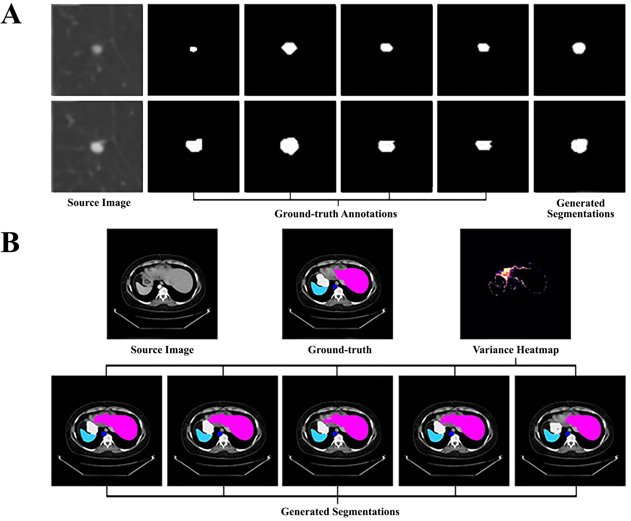
Figure 2: Generative Segmentation of Medical Images with VAE U-net. A) Generated Lung cancer segmentation from LIDC-IRDI dataset. It is able to provide a plausible boundary based on four ground truth segmentations. B) Segmentation of abdominal organs on Synapse dataset with the variance heatmap. The variance heatmap is derived from multiple sampled segmentations.

4.2.2 Qualitative Study of the Uncertainty Map

After drawing multiple segmentations from the latent space using VAE U-net, we can generate a segmentation uncertainty map by calculating the pixel-wise variance of predicted segmentations and normalizing it by the maximum value of variance among the samples, illustrated by the bottom panel of Figure 2. We demonstrate the use of this uncertainty map for the out-of-distribution detection task. Out-of-distribution samples are constructed using three different ways: 1) applying Gaussian blurring to the image; 2) adding a patch to a random location in the image; 3) using abnormal samples from PMC Open Access Subset [9]. Figure 3 visualizes the uncertainty maps for the three cases. For Gaussian blurred images, the map highlights the uncertainty near the anatomical boundaries. For random patched image or abnormal image with liver tumour, the map highlights the location of abnormalities. The ability of uncertainty measurement can serve as a potentially powerful tool for further downstream tasks.

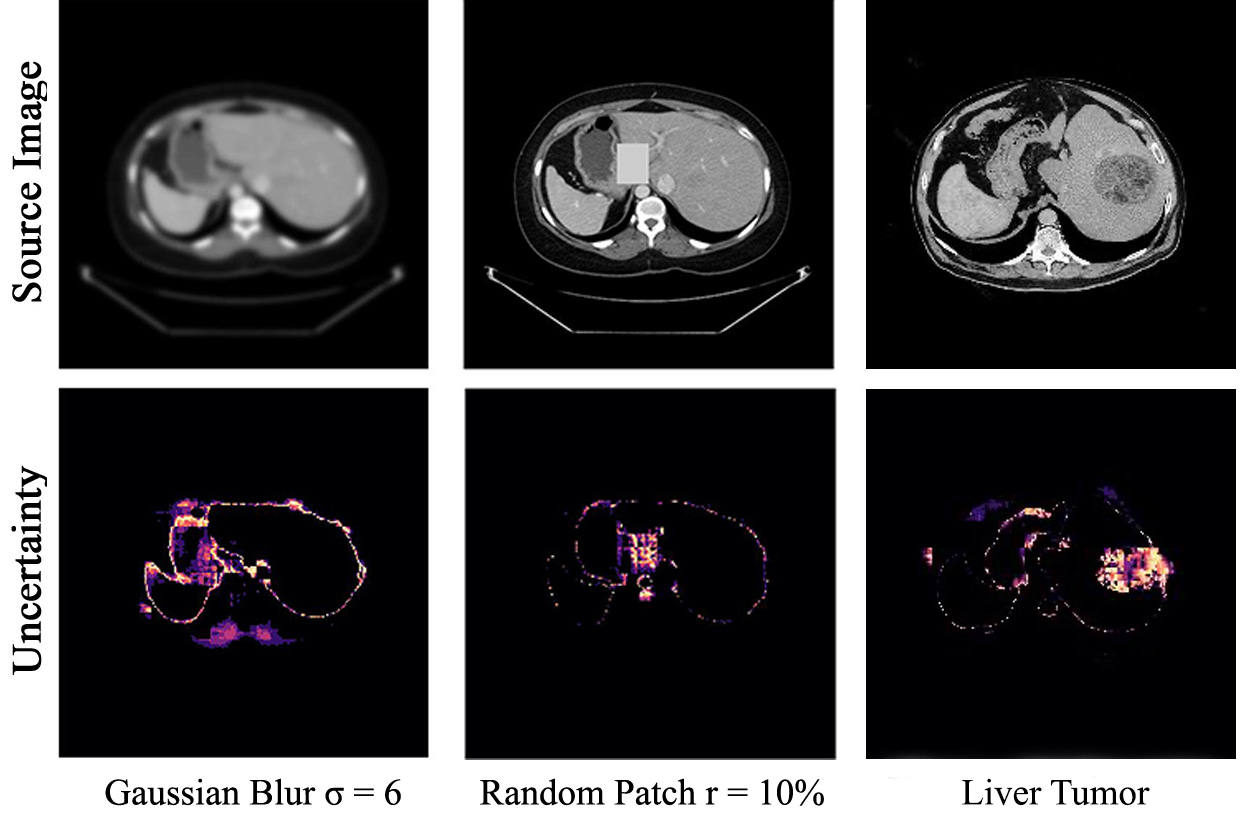
Figure 3: Uncertainty heatmap for out-of-distribution detection. The heatmap is generated from 10 segmentation maps from VAE U-net. Brighter color means more disagreement (variance) in generated segmenatations and vice versa. Random patching adds a $r=10\%$ patch which is proportional to 10% of the image size.

4.2.3 Quantitative Metrics for Segmentation Performance

Table 2 compares the segmentation performance of the proposed method to state-of-the-art deep learning methods on the Synapse dataset. The proposed VAE U-net was used in two modes: the sampling mode which generates a number of plausible segmentations and the prior mode which generates a single segmentation using the prior mean. Both modes show a strong performance compared to existing methods. VAE U-net in prior mode achieves the highest overall Dice score of 78.71% on Dice score and the highest overall Hausdorff distance (HD) of 20.86mm. It also achieved the best score for the kidney and stomach. In sampling mode, the sampled segmentations achieve $77.29\%(\pm 0.22\%)$ in Dice and $26.52\text{mm}(\pm 1.65\text{mm})$ in HD, which are in line with other state-of-the-art methods, indicating the usefulness of incorporating uncertainty into segmentation. The bottom panel of Figure 2 shows the visualization of the segmentations as well as the variance on selected samples.

Methods	Dice $\uparrow$	HD $\downarrow$	Aorta	Gallbladder	Kidney(L)	Kidney(R)	Liver	Pancreas	Spleen	Stomach
V-Net	68.81	-	75.34	51.87	77.10	80.75	87.84	40.05	80.56	56.98
DARR	69.77	-	74.74	53.77	72.31	73.24	94.08	54.18	89.90	45.96
R50 U-Net	74.68	36.87	87.74	63.66	80.60	78.19	93.74	56.90	85.87	74.16
U-Net	76.85	39.70	89.07	69.72	77.77	68.60	93.43	53.98	86.67	75.58
R50 Att-Unet	75.57	36.97	55.92	63.91	79.20	72.71	93.56	49.37	87.19	74.95
Att-Unet	77.77	36.02	89.55	68.88	77.98	71.11	93.57	58.04	87.30	75.75
R50 ViT	71.29	32.87	73.73	55.13	75.80	72.20	91.51	45.99	81.99	73.95
TransUnet	77.48	31.69	87.23	63.13	81.87	77.02	94.08	55.86	85.08	75.62
SwinUnet	78.39	24.73	86.65	66.15	83.71	79.89	93.87	56.00	87.98	72.88
VAE U-net (Sample)	77.29 $\pm$ 0.22	26.52 $\pm$ 1.65	83.99 $\pm$ 0.22	63.37 $\pm$ 0.74	82.93 $\pm$ 0.49	78.42 $\pm$ 0.46	93.59 $\pm$ 0.06	53.38 $\pm$ 0.55	88.78 $\pm$ 0.30	73.83 $\pm$ 0.41
VAE U-net (Prior)	78.71	20.86	85.40	65.01	83.96	80.16	93.89	55.42	89.65	76.18

Table 2: Segmentation performance on Synapse test set. The second and third columns report the average performance across organs. The mean and variance in sampling mode is calculated from 10 generated segmentations sampled from the prior latent distribution.

5 Conclusion

In this paper, we proposed a novel uncertainty measurement method for Unet-based image segmentation models, named as VAE U-net. VAE U-net models uncertainty via the skip connection and thus is potentially applicable to other segmentation models that consist of multi-level skip connections. The proposed method achieves a high segmentation performance compared to state-of-the-art deterministic models, as well as to a high uncertainty estimation capability compared to uncertainty-aware segmentation models in terms of generalised energy distance and normalized cross correlation score. By drawing multiple plausible segmentations from the latent space, the proposed method can generate an uncertainty map for the segmentation, which not only facilitates the detection of out-of-distribution samples with noise and abnormality, but also provide an extra layer of interpretability to the segmentation.

Appendix

Appendix 0.A Model Output and Visualization for Synapse Dataset

In the paper, we quantitively evaluate model performance with the sampled latent space with the prior distribution. The detailed metrics for each sample are shown in Table 3.

Sample	Aorta		Gallbladder		Kidney(L)		Kidney(R)		Liver		Pancreas		Spleen		Stomach
	DSC	HD	DSC	HD	DSC	HD	DSC	HD	DSC	HD	DSC	HD	DSC	HD	DSC	HD
1	0.8366	10.8351	0.6369	42.0419	0.8309	35.9437	0.7920	48.9854	0.9356	21.1717	0.5280	13.7971	0.8883	30.1600	0.7416	18.1989
2	0.8447	7.5771	0.6371	28.9042	0.8297	32.5005	0.7843	56.9210	0.9360	21.3996	0.5283	13.3646	0.8888	36.6232	0.7423	16.8864
3	0.8394	9.4634	0.6377	36.7390	0.8267	32.9405	0.7835	48.2171	0.9364	20.1728	0.5394	13.9482	0.8872	32.2708	0.7366	19.1086
4	0.8370	10.6003	0.6416	34.6728	0.8283	33.6209	0.7863	51.2560	0.9364	20.6927	0.5250	14.1900	0.8847	24.5469	0.7367	17.6837
5	0.8422	7.9080	0.6394	37.1049	0.8298	39.9077	0.7913	44.3016	0.9358	20.9809	0.5303	13.9811	0.8908	23.4351	0.7422	17.6694
6	0.8392	11.5661	0.6457	42.0551	0.8313	43.2612	0.7757	52.3549	0.9361	20.7980	0.5281	14.0435	0.8911	21.3762	0.7429	16.8955
7	0.8360	10.1318	0.6150	43.8266	0.8227	38.1155	0.7798	51.0938	0.9349	20.8692	0.5291	13.3467	0.8876	33.1373	0.7324	17.3859
8	0.8416	9.3573	0.6268	35.4166	0.8343	32.0674	0.7827	37.2433	0.9352	22.7996	0.5427	13.4555	0.8865	26.1281	0.7384	17.6222
9	0.8384	9.9281	0.6243	43.1226	0.8347	31.3610	0.7891	37.8275	0.9370	21.1330	0.5359	12.9866	0.8919	23.7895	0.7441	17.2179
10	0.8388	8.8284	0.6314	36.4831	0.8295	35.0589	0.7807	43.4456	0.9359	26.7443	0.5423	13.3481	0.8816	26.4568	0.7360	16.6224
11	0.8393	10.1432	0.6250	44.0193	0.8364	31.6526	0.7892	47.2165	0.9353	20.9640	0.5378	13.2315	0.8864	37.1440	0.7407	17.0977
12	0.8377	10.4850	0.6367	38.5701	0.8353	35.5516	0.7871	54.8652	0.9352	22.0824	0.5358	13.3616	0.8861	26.5290	0.7395	17.3862
13	0.8401	7.5355	0.6306	43.4111	0.8243	32.4223	0.7800	60.8630	0.9359	20.2417	0.5349	13.8721	0.8865	22.4895	0.7266	18.0815
14	0.8377	9.5309	0.6326	29.2546	0.8232	41.4945	0.7823	54.1239	0.9365	20.9434	0.5293	13.7607	0.8911	19.2319	0.7371	16.6482
15	0.8408	12.2123	0.6317	34.6952	0.8319	33.1501	0.7892	44.0921	0.9370	20.6693	0.5360	14.1194	0.8920	25.7182	0.7381	17.2505
16	0.8390	10.3945	0.6285	35.8092	0.8289	36.4739	0.7872	43.1464	0.9347	21.9926	0.5276	13.7141	0.8849	25.9178	0.7311	18.3067
17	0.8433	7.7038	0.6214	43.8646	0.8323	32.6734	0.7884	50.8036	0.9366	20.8931	0.5386	14.2091	0.8855	23.8639	0.7431	16.0795
18	0.8397	13.0554	0.6484	41.6519	0.8238	36.3828	0.7710	70.8122	0.9357	25.2957	0.5278	13.5820	0.8854	28.7111	0.7381	18.1320
19	0.8397	10.1656	0.6290	35.6434	0.8227	32.5431	0.7767	68.4746	0.9358	21.8821	0.5381	13.7800	0.8804	26.7668	0.7345	17.3851
20	0.8444	6.8438	0.6415	35.0602	0.8349	31.7220	0.7882	42.0353	0.9362	21.2437	0.5398	13.7009	0.8895	24.7836	0.7402	19.3254
21	0.8402	9.3683	0.6403	35.1964	0.8324	31.6422	0.7856	42.2339	0.9351	33.4777	0.5363	14.0311	0.8868	29.1294	0.7448	17.4502
22	0.8415	8.1393	0.6246	36.0243	0.8388	33.4439	0.7856	35.7542	0.9353	24.3854	0.5323	14.5034	0.8913	25.0883	0.7415	17.0907
23	0.8398	9.8867	0.6386	43.7625	0.8364	31.5464	0.7876	48.1456	0.9361	22.9412	0.5437	13.6355	0.8919	24.6596	0.7403	17.5962
24	0.8400	8.9493	0.6377	43.7889	0.8291	34.2538	0.7841	35.4504	0.9368	22.6263	0.5375	13.9456	0.8909	22.9949	0.7377	17.7307
25	0.8379	11.1249	0.6262	43.8527	0.8248	37.3052	0.7816	63.9425	0.9365	20.5847	0.5302	13.9278	0.8861	26.2930	0.7401	18.0096
26	0.8411	11.7145	0.6366	35.3857	0.8263	33.3029	0.7843	27.9618	0.9358	23.4411	0.5207	14.4669	0.8864	24.8067	0.7397	16.8104
27	0.8428	10.4767	0.6346	37.0661	0.8254	43.4891	0.7809	45.0421	0.9350	27.0051	0.5361	13.4993	0.8851	33.3704	0.7334	16.8366
28	0.8417	8.2642	0.6332	35.6866	0.8173	41.7104	0.7804	47.2405	0.9365	20.7961	0.5332	13.8991	0.8879	25.6882	0.7324	17.0354
29	0.8403	7.7829	0.6367	30.3253	0.8267	40.9993	0.7853	47.4382	0.9355	20.1965	0.5322	14.0804	0.8911	24.6459	0.7390	17.1018
30	0.8374	10.8176	0.6419	36.5570	0.8289	44.0330	0.7845	55.7831	0.9358	22.0614	0.5370	14.5356	0.8897	22.5841	0.7389	16.9006

Table 3: Model Performance Metrics for 30 Sampled Annotations using Prior Distribution on Synapse Dataset.

In Synapse dataset, the degree of uncertainty largely depends on the slice position. When the slices are closer to the boundary of the organs, the model becomes uncertain about the correct segmentation of the source image. Figure 4 is the generated segmentations for test case 35 (slice 80). We can see the boundary of the organs in the uncertainty magma colour map, which is the variance of the segmentation map (20 in total). In this case, there is little ambiguity in the target segmentation, therefore the generated segmentations look similar.

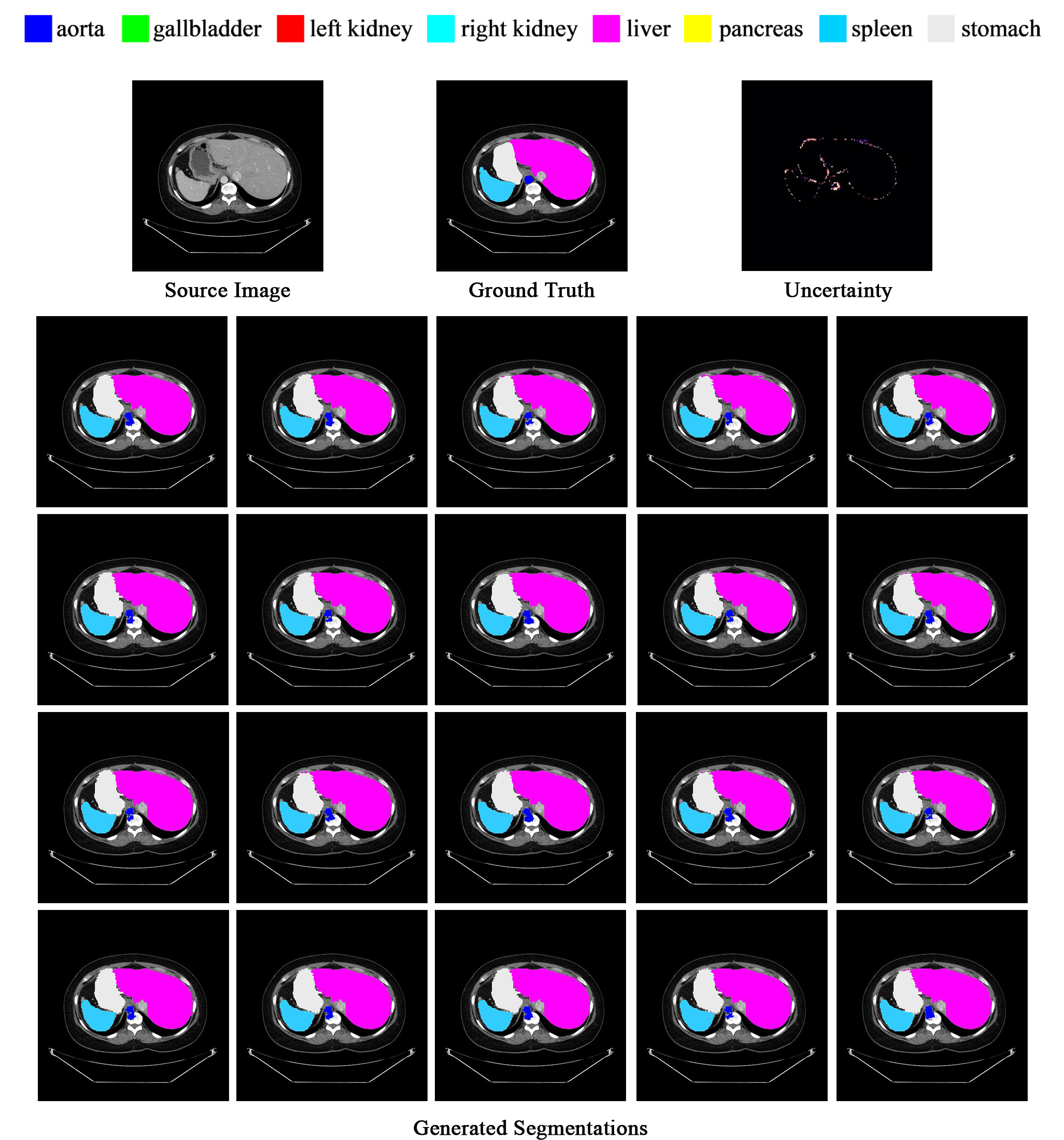
Figure 4: Visualization of Generated Samples with Uncertainty on Synapse dataset Test Case 35 (Slice 80).

For the same test case but with a different slice position, the ambiguity increases as the boundaries between organs become blurry. For slice 84, the visualized samples are shown in Figure 5. It is clear that the area around the liver in the source image stops the human grader to mark it precisely, but the model can generate different reasonable samples in the learning process and produces high uncertainty measurements around this area.

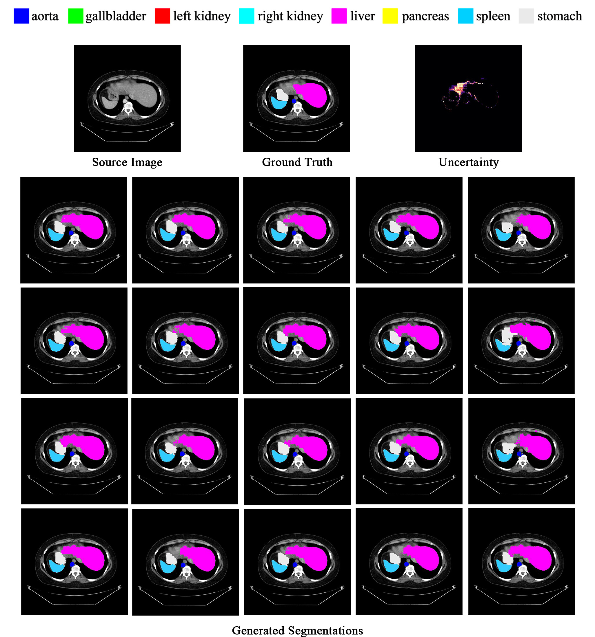
Figure 5: Visualization of Generated Samples with Uncertainty on Synapse dataset Test Case 35 (Slice 84).

To comprehensively compare the fidelity of the reconstruction, we picked three previous state-of-the-art Unet-like models to compare against our approach. Three ambiguous segmentation samples are selected from test case 22 (slice 61), test case 22 (slice 66) and test case 2 (slice 106) to visualize the overlaid segmentation map. The result is shown in Figure 6.

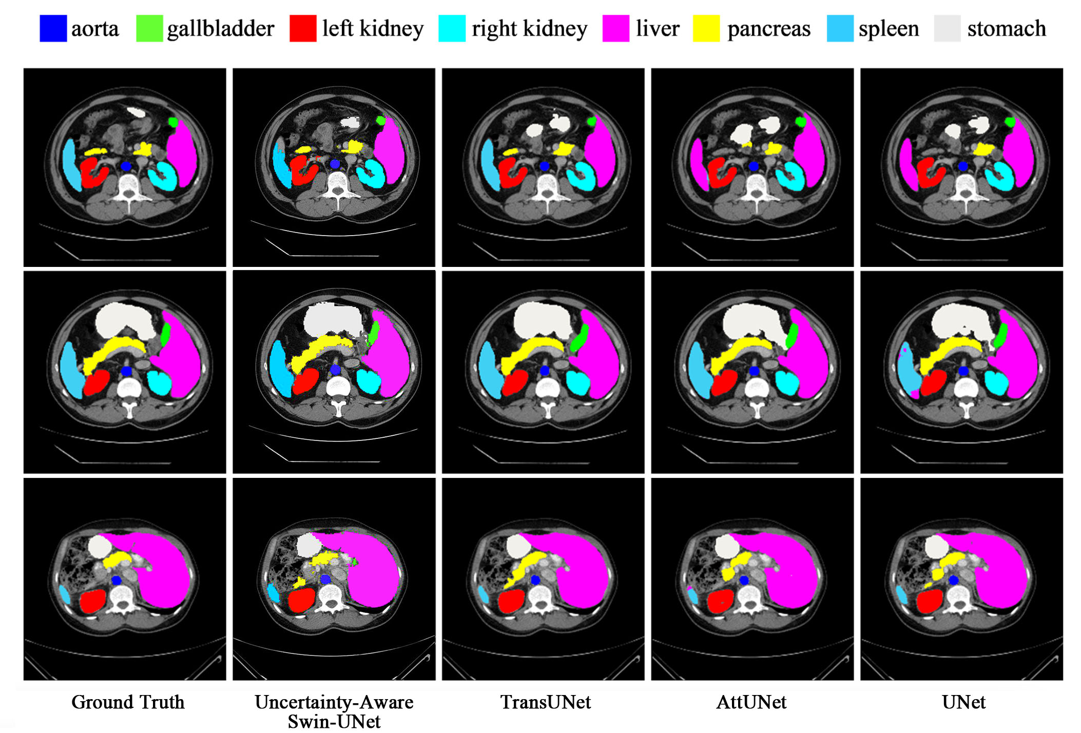
Figure 6: Comparison of Segmentation Results on Synapse Dataset. Models for comparison are TransUnet [7], AttnUnet [17] and Unet [18].

Appendix 0.B Model Prediction Visualization for LIDC Dataset

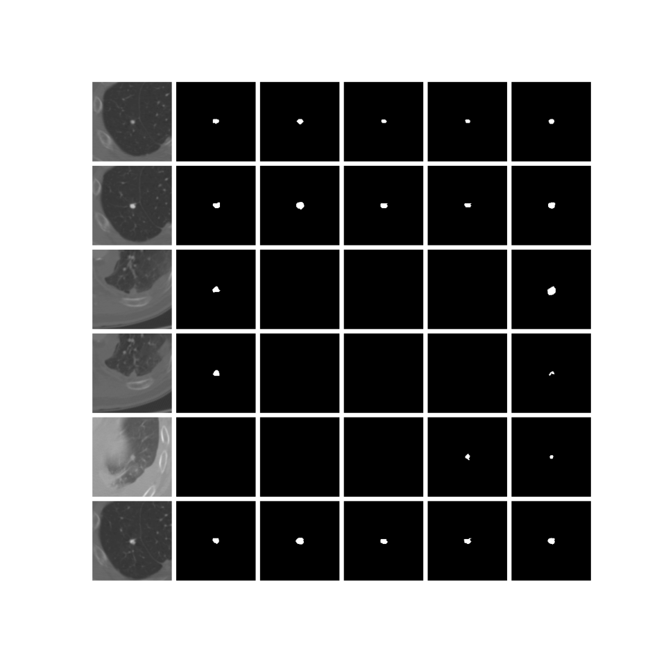
Figure 7: Visualization of 5 Predicted Annotations using Prior Sampling on LIDC Dataset Case 0021.

Appendix 0.C Network Hyper-parameters

The hyper-parameters that are being used for training is shown in Table 4. During training, we used a combination of cross-entropy loss and the Dice-Similarity coefficient (Dice) loss. The former term can quickly guide the network to learn general segmentation and the latter one comes into effect when learning the fine details. We also used a decayed learning rate scheduler with $1\times 10^{-4}$ decay rate. To balance the magnitude of variance, we used a relatively small $\beta=0.1$ and use the average of KL-divergence from all levels in (14) to keep the scale consistent with the reconstruction loss.

Parameter	Value
Batch Size	24
Learning Rate	0.05 (Synapse)/ 0.01 (LIDC)
Input Size	[224, 224]
Output Size	[512, 512]
Momentum	0.9
Weight Decay	0.0001
Reconstruction Loss	Cross-Entropy (0.4) + Dice (0.6)
Epoch	150
KL-divergence $\beta$	0.1

Table 4: Model Training Hyper-parameters.

Appendix 0.D Computational Complexity

Apart from the performance perspectives, we also want to investigate the performance of the given model. Because of the use of windowed transformer modules, our method is significantly faster than raw transformer-based or convolutional-based models. Compared to the previous state-of-the-art Swin-Unet model, our model can achieve higher accuracy with minimal additional cost on the total number of parameters and FLOPs. With the extra cost of 0.02% (3.6K) parameters, we can improve the overall Dice performance by 0.32% and overall HD score by 15.64%, which demonstrated the importance of uncertainty modeling in medical image segmentation tasks.

The complexity of popular models in medical image segmentation is shown in Table 5. From the table, we can see that our method holds a small number of parameters as well as a small number of flops. The computational efficiency of the model is largely attributed to the tiny design of the Swin-Transformer block we adopted. With the shifted and patched windows attention module, it is significantly more efficient than its competitors. Although our model is similar to nnUnet in terms of the number of parameters, we have approximately $1\%$ of its flops which greatly accelerate the inference time.

Methods	# of Params (M) $\downarrow$	FLOPs (G) $\downarrow$	Inference Time (s) $\downarrow$
TransUnet	$96.07$	$48.34$	$26.97$
nnUnet	$19.07$	$412.65$	$10.28$
CoTr	$46.51$	$399.21$	$19.21$
ASPP	$47.92$	$44.87$	$25.47$
SETR	$86.03$	$43.49$	$24.86$
Our Method	$20.08$	$4.92$	$0.25$

Table 5: Computational Complexity of Synapse Segmentation Models.

The small number of flops greatly benefit the application of this model with rapid inference and testing. Using the Swin-T backbone, we can sample in the inference stage while having a reasonable waiting time for patients. Compared to previous methods, we can generate nearly 50 samples before previous models can generate one single prediction.

Appendix 0.E Figures for Out-of-distribution Detection

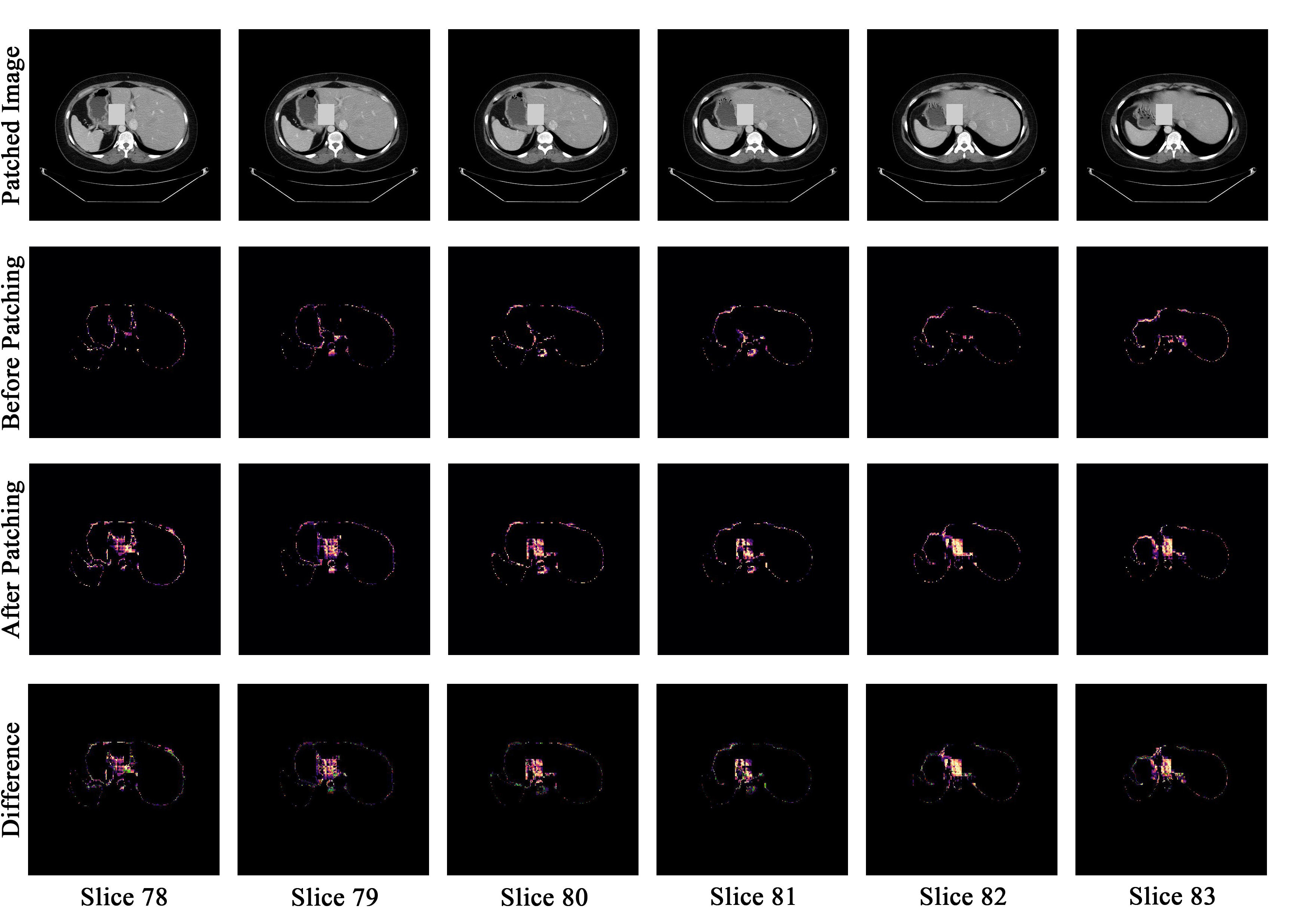
Figure 8: Qualitative Study of Randomly Patched Samples on Synapse dataset Test Case 35. The variance of the predicted 20 samples is visualized in magma colormap.

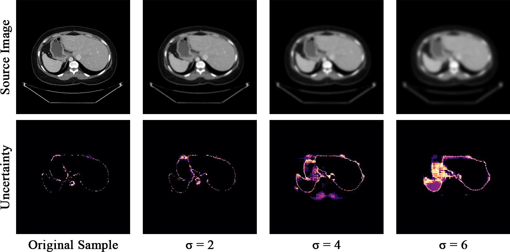
Figure 9: Qualitative Study of the Impact of Gaussian Blur Filters ($\sigma$) on Synapse dataset Test Case 35 (Slice 80). The variance of the predicted 20 samples is visualized in magma colormap.

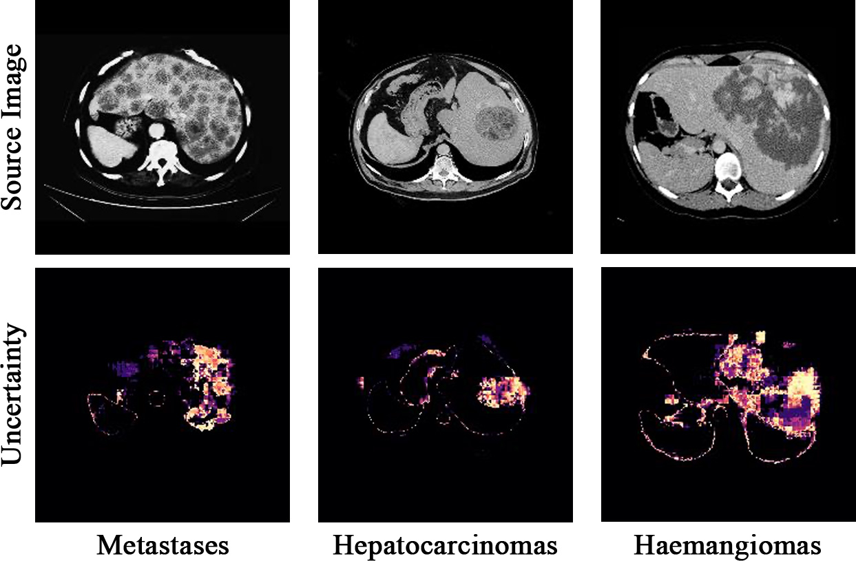
Figure 10: Qualitative Study of Real Liver Tumor. The variance of the predicted 20 samples is visualized in magma colormap.

Appendix 0.F Latent Space Visualization

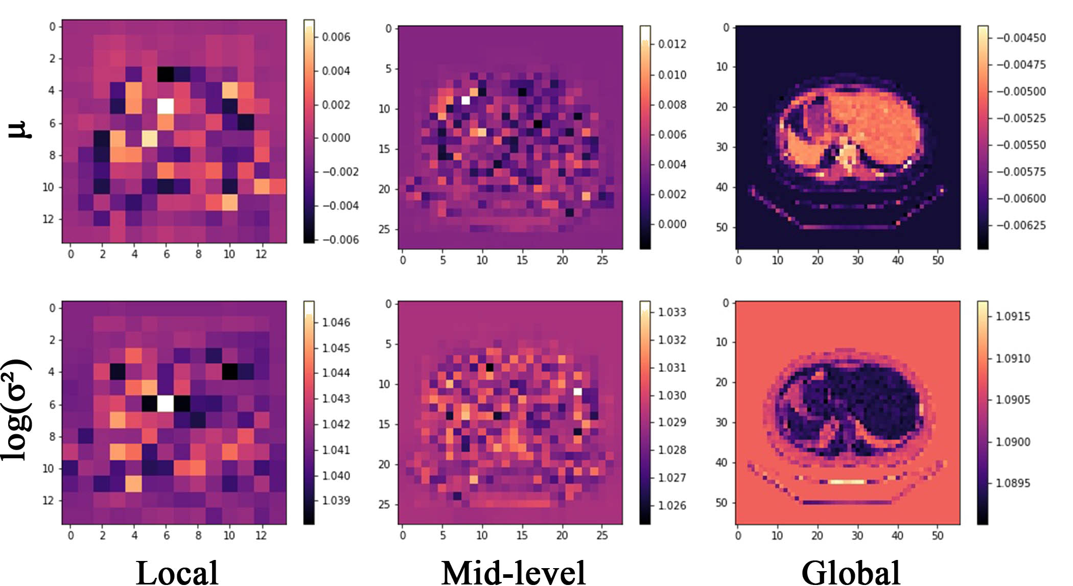
Figure 11: Visualization of mean $\mu$ and variance $\log(\sigma^{2})$ in Gaussian Latent Space across 3 Levels on Synapse dataset Test Case 35 (Slice 80).

References

- [1] Synapse multi-organ segmentation dataset: Multi-atlas labeling beyond the cranial vault - Workshop and Challenge. https://www.synapse.org/#!Synapse:syn3193805/wiki/217789, accessed: 2022-09-30
- [2] Abdar, M., Pourpanah, F., Hussain, S., Rezazadegan, D., Liu, L., Ghavamzadeh, M., Fieguth, P., Cao, X., Khosravi, A., Acharya, U.R., Makarenkov, V., Nahavandi, S.: A review of uncertainty quantification in deep learning: Techniques, applications and challenges. Information Fusion 76, 243–297 (dec 2021). https://doi.org/10.1016/j.inffus.2021.05.008, https://doi.org/10.1016%2Fj.inffus.2021.05.008
- [3] Armato III, S.G., McLennan, G., Bidaut, L., McNitt-Gray, M.F., Meyer, C.R., et al.: The lung image database consortium (LIDC) and image database resource initiative (IDRI): a completed reference database of lung nodules on CT scans. Medical Physics (2011)
- [4] Baumgartner, C.F., Tezcan, K.C., Chaitanya, K., Hötker, A.M., Muehlematter, U.J., et al.: PHiSeg: Capturing uncertainty in medical image segmentation. In: Medical Image Computing and Computer Assisted Intervention (2019)
- [5] Begoli, E., Bhattacharya, T., Kusnezov, D.: The need for uncertainty quantification in machine-assisted medical decision making. Nature Machine Intelligence 1(1), 20–23 (2019)
- [6] Cao, H., Wang, Y., Chen, J., Jiang, D., Zhang, X., Tian, Q., Wang, M.: Swin-unet: Unet-like pure transformer for medical image segmentation. arXiv preprint arXiv:2105.05537 (2021)
- [7] Chen, J., Lu, Y., Yu, Q., Luo, X., Adeli, E., Wang, Y., Lu, L., Yuille, A.L., Zhou, Y.: TransUnet: Transformers make strong encoders for medical image segmentation. arXiv:2102.04306 (2021)
- [8] Gal, Y., Ghahramani, Z.: Dropout as a Bayesian approximation: Representing model uncertainty in deep learning. In: International Conference on Machine Learning (2016)
- [9] Gamble, A.: Pubmed central (pmc). The Charleston Advisor 19(2), 48–54 (2017)
- [10] Graves, A.: Practical variational inference for neural networks. Advances in neural information processing systems 24 (2011)
- [11] Higgins, I., Matthey, L., Pal, A., Burgess, C.P., Glorot, X., et al.: beta-VAE: Learning basic visual concepts with a constrained variational framework. In: International Conference on Learning Representations (2017)
- [12] Kingma, D.P., Welling, M.: An introduction to variational autoencoders. Foundations and Trends in Machine Learning (2019)
- [13] Kohl, S., Romera-Paredes, B., Meyer, C., De Fauw, J., Ledsam, J.R., et al.: A probabilistic u-net for segmentation of ambiguous images. Advances in Neural Information Processing Systems (2018)
- [14] Kohl, S.A.A., Romera-Paredes, B., Maier-Hein, K.H., Rezende, D.J., Eslami, S.M.A., Kohli, P., Zisserman, A., Ronneberger, O.: A hierarchical probabilistic u-net for modeling multi-scale ambiguities. CoRR abs/1905.13077 (2019), http://arxiv.org/abs/1905.13077
- [15] Kohl, S.A., Romera-Paredes, B., Maier-Hein, K.H., Rezende, D.J., Eslami, S., et al.: A hierarchical probabilistic U-net for modeling multi-scale ambiguities. Medical Imaging meets NeurIPS (2019)
- [16] Lakshminarayanan, B., Pritzel, A., Blundell, C.: Simple and scalable predictive uncertainty estimation using deep ensembles. Advances in Neural Information Processing Systems (2017)
- [17] Oktay, O., Schlemper, J., Folgoc, L.L., Lee, M., Heinrich, M., Misawa, K., Mori, K., McDonagh, S., Hammerla, N.Y., Kainz, B., Glocker, B., Rueckert, D.: Attention u-net: Learning where to look for the pancreas. In: Medical Imaging with Deep Learning (2018)
- [18] Ronneberger, O., Fischer, P., Brox, T.: U-net: Convolutional networks for biomedical image segmentation. In: Medical Image Computing and Computer-Assisted Intervention (2015)
- [19] Srivastava, N., Hinton, G., Krizhevsky, A., Sutskever, I., Salakhutdinov, R.: Dropout: a simple way to prevent neural networks from overfitting. Journal of Machine Learning Research (2014)
- [20] Wen, Y., Vicol, P., Ba, J., Tran, D., Grosse, R.: Flipout: Efficient pseudo-independent weight perturbations on mini-batches. International Conference on Learning Representations (2018)
- [21] Zhao, Y., Yang, C., Schweidtmann, A., Tao, Q.: Efficient Bayesian uncertainty estimation for nnU-Net. In: Medical Image Computing and Computer-Assisted Intervention (2022)