Gravitational Wave Emission from a Cosmic String Loop, I: Global Case

Abstract

We study the simultaneous decay of global string loops into scalar particles (massless and massive modes) and gravitational waves (GWs). Using field theory simulations in flat space-time of loops with initial length $\sim 80-1700$ times their core width, we determine the power emitted by a loop into scalar particles, $P_{\varphi}$, and GWs, $P_{\rm GW}$, and characterize the loop-decay timescale as a function of its initial length, energy and angular momentum. We quantify infrared and ultraviolet lattice dependencies of our results. For all type of loops and initial conditions considered, GW emission is always suppressed compared to particles as $P_{\rm GW}/P_{\varphi}\simeq\mathcal{O}(10)(v/m_{\text{p}})^{2}\ll 1$, where $v$ is the vacuum expectation value associated with string formation. Our results suggest that the GW background from a global string network, such as in dark matter axion scenarios, will be highly suppressed.

Motivation.– Cosmic string networks [1] are predicted by a variety of field theory and superstring early Universe scenarios [1, 2, 3, 4, 5, 6, 7]. They consist primarily of ‘long’ (infinite) strings stretching across the observable universe, and string loops. The long-string density decreases as they intercommute forming loops. In the Nambu-Goto (NG) approximation of infinitely thin strings, loops decay mainly into gravitational waves (GWs), leading to a stochastic GW background (GWB) [8, 9, 10].

While LIGO and VIRGO have placed stringent constraints on the cosmic string GWB at $\sim 10-100$ Hz frequencies [11, 12], recently, pulsar timing array (PTA) collaborations [13, 14, 15, 16] have announced the first evidence for a GWB, at the $\sim$ nHz frequency window. Although a GWB from a population of supermassive black hole binaries (SMBHBs) is naturally expected at the PTA frequencies [17, 18], cosmological backgrounds also represent a viable explanation [19, 18, 20], in particular, a cosmic (super)string [21, 5] GWB [19, 18, 20, 22, 23, 24, 25, 26]. Fitting the PTA data with a signal from NG cosmic strings leads to a tight constraint on the string tension, $\sqrt{\mu}\simeq 1.32^{+0.20}_{-0.24}\times 10^{14}~{}{\rm GeV}$ [20]. The fit to the data is however not as good as for SMBHB or other cosmological signals [19, 18, 20]. A cosmic superstring network, on the other hand, provides a better fit to the PTA data [19, 18, 20], accommodating a smaller string energy scale as $\sqrt{\mu}\simeq 1.56^{+0.48}_{-0.39}\times 10^{13}~{}{\rm GeV}$, while suppressing the string intercommutation probability down to $p\sim 0.001-0.007$ [20]. The potential detection of a signal from string networks in the mHz-kHz window by next generation GW detectors like LISA [27], and others [28], with tensions down to $\sqrt{\mu}\gtrsim 10^{10}$ GeV [29], adds further opportunity to detect a string network.

Given these exciting developments, a revisit of the GW signal calculation from cosmic strings seems in order. A crucial aspect which remains to be resolved is to understand whether GWs are in fact the key decay channel of cosmic strings. Being primarily field theory objects, a natural decay route is particle production from the fields themselves, and [30, 31] have argued that this is the primary decay path for Abelian-Higgs strings. Recently, [32] set up and evolved Abelian-Higgs loop configurations, comparing the observed particle production in their set-up with the traditional GW result from NG loops. For loops below a critical length, they found decay primarily through particle production, whilst for larger loops GW emission dominates. In [33] they extended their work, considering the decay of global string loops into massless and massive scalar modes.

In this Letter we extend the approach taken in [33], with one important addition: a true comparison of the relative decay into GWs and particle production requires both processes happening simultaneously. Here we do just that, using global loops created either via the algorithm of [33] or directly from networks as in [34, 35]. Our main result is that for all shapes of the global loops (e.g. ‘squared’, ‘circular’, ‘twisted’) and types of initial conditions considered (e.g. initial length, energy, angular momentum), the power emitted in GWs is suppressed compared to particle emission as $P_{\rm GW}/P_{\varphi}\simeq\mathcal{O}(10)(v/m_{\text{p}})^{2}\ll 1$, with $v$ the vacuum expectation value ($vev$) associated to string formation. An analogous study for Abelian-Higgs strings will appear later.

Loop configurations.– We consider a model with a complex scalar field, $\varphi=(\phi_{1}+i\phi_{2})/\sqrt{2}$, and action

$$S=-\int\text{d}^{4}x\sqrt{-g}\left[\partial_{\mu}\varphi^{*}\partial^{\mu}\varphi+V(\varphi)\right],$$ (1)

where $V(\varphi)=\lambda(\varphi\varphi^{*}-v^{2}/2)^{2}$. This model exhibits two phases: a symmetric phase with $\langle\varphi\rangle=0$, and a broken phase with $\langle\varphi^{*}\varphi\rangle=v^{2}/2$, where both massless ($\theta$) and massive ($\chi$) excitations of mass $m_{\chi}=\sqrt{2\lambda}v$ are present. If a transition from the unbroken to the broken phase takes place, global strings form. These are line-like topological defects with long-range interactions and a core of radius $r_{\text{c}}\sim 1/m_{\chi}$ trapped in the symmetric phase.

We study the decay of global string loops in flat space-time using lattice simulations performed with $\mathcal{C}$osmo$\mathcal{L}$attice ($\mathcal{C}\mathcal{L}$) [36, 37]. The GW emission is obtained with the GW-module of $\mathcal{C}\mathcal{L}$ [38], based on [39]. We use lattices with periodic boundary conditions, side length $L$, $N$ sites per dimension, and lattice spacing $\delta x=L/N$. We monitor the loop dynamics by measuring relevant observables: the energy and spectra of the $\theta$ and $\chi$ modes [33, 40], and the loop’s length, energy [35] and angular momentum [33], with the latter two defined as

$$E_{\text{str}}=\int\text{d}^{3}x\,W(\varphi)\left[\dot{\varphi}\dot{\varphi}^{*}+\vec{\nabla}\varphi\cdot\vec{\nabla}\varphi^{*}+V(\varphi)\right]\,,$$ (2)

$$\vec{J}=-\frac{1}{2}\int\text{d}^{3}x\,W(\varphi)\left[\vec{x}\times\big{(}\dot{\varphi}\vec{\nabla}\varphi^{*}+\dot{\varphi}^{*}\vec{\nabla}\varphi\big{)}\right]\,,$$ (3)

with $W(\varphi)=(V(\varphi)/W_{0})\times\Theta(v^{2}/2-|\varphi|^{2})$ a weight function, $W_{0}=\lambda v^{4}/4$ and $\Theta(x)$ the step function. We consider two type of loops, i) network loops originating from the decay of string networks, and ii) artificial loops forming from the intersection of infinite straight strings.

Network loops. Following [35] we initially create a Gaussian random realization of $\varphi$ with given correlation length $\ell_{\text{str}}$. The field first undergoes a diffusive phase to obtain a smooth string configuration, which is then evolved in a radiation-dominated (RD) background with the string-core resolution-preserving approach of [41], until the system is close to its scaling regime [42, 43, 44]. The resulting network is finally evolved in flat space-time until it decays into a single isolated loop, which represents the initial condition for our study. Initial netwonetwork loop lengths range between $\sim(0.5-6)L$. Note that only $\sim 35\%$ of the network simulations lead to isolated loops, of which only $\sim 40\%$ are useful for our study, as we discard those simulations for which the loop intercommutes to form infinite strings, attracts itself around the box preventing its decay, or is much longer than the box size.

Artificial loops. Following [33] we create loops from the intersection of two perpendicular pairs of boosted infinite strings [45], each pair separated by a distance $L_{1/4}$ and modified to obey periodic boundary conditions [33]. The initial two-pair configuration is characterized by $L_{1/4}$, the boost velocities of each pair, $v_{1}$ and $v_{2}$, and an angle $\alpha$ between the boost direction and normal to the plane where the loops intersect, see Fig. S2. This method leads to the formation of two squared loops, an inner and an outer one. Shortly after intersection, the two loops begin to shrink, moving apart from each other. We isolate the inner loop, substituting the field outside a cylindrical volume that encompasses this loop by a smooth and periodic configuration which continuously matches $\varphi$ and $\dot{\varphi}$ in the surface of the cylinder. This results in a single isolated loop with length $L_{0}\approx 4L_{1/4}$ (slightly smaller in reality). Unlike for network loops, we can control $L_{0}$ by appropriately choosing $L_{1/4}$ (typically as a fraction of $L$).

For more details on how loops are generated, see supplemental material. Observables will be expressed, from now on, in terms of dimensionless program variables: $\tilde{\varphi}=\varphi/v$, $\tilde{\vec{x}}=\sqrt{\lambda}v\,{\vec{x}}$, $\tau=\sqrt{\lambda}v\,t$, $\kappa=k/\sqrt{\lambda}v$, ${\tilde{E}}_{\text{str,0}}=(\sqrt{\lambda}/v)\,E_{\text{str,0}}$, and $\tilde{J}_{0}=\lambda|\vec{J}_{0}|$.

String loop	$A\times 10^{3}$	$B$	$C\times 10^{3}$	$D$
Network loops	$185\pm 22$	$5\pm 14$	$70\pm 12$	$15\pm 17$
$v_{1}=0.9,v_{2}=0.9$	$571\pm 10$	$-26\pm 3$	$270\pm 9$	$-22\pm 6$
$v_{1}=0.9,v_{2}=0.6$	$430\pm 30$	$-13\pm 11$	$223\pm 14$	$-14\pm 9$
$v_{1}=0.9,v_{2}=0.3$	$534\pm 14$	$-23\pm 5$	$269\pm 9$	$-20\pm 6$
$v_{1}=0.9,v_{2}=0.0$	$706\pm 19$	$-45\pm 6$	$348\pm 9$	$-40\pm 6$
$v_{1}=0.6,v_{2}=0.6$	$227\pm 11$	$-3\pm 4$	$125\pm 5$	$-1\pm 3$
$v_{1}=0.6,v_{2}=0.3$	$260\pm 15$	$-9\pm 5$	$140\pm 8$	$-6\pm 5$
$v_{1}=0.3,v_{2}=0.3$	$280\pm 30$	$-1\pm 9$	$154\pm 15$	$2\pm 9$

Table 1: Coefficients of linear fits $\Delta\tau_{\rm dec}=A\tilde{L}_{0}+B$ and $\Delta\tau_{\rm dec}=C\tilde{E}_{\text{str,0}}+D$.

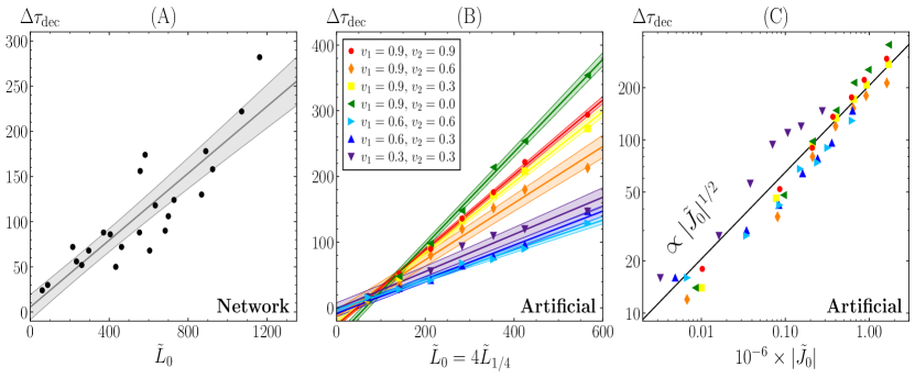
Figure 1: Lifetime as a functions of initial length for network (A) and artificial loops with different boost velocities (B), and as a function of initial angular momentum for the artificial loops (C), in a logarithmic scale. Lines and shaded regions in (A) and (B) correspond to linear-fit results, while the line in (C) is not a fit.

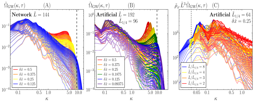
Figure 2: GW energy density spectra evolution for network (A) and artificial loops (B) with varying UV resolution, $\delta\tilde{x}$, and fixed lattice size, $\tilde{L}$, and for artificial loops with varying the IR scale $\tilde{L}$ while fixing $\delta\tilde{x}$ (C). Dashed vertical lines indicate the scale of the string width, $\kappa_{\text{c}}=2\pi/\tilde{r}_{\text{c}}$, while the dotted vertical line indicates the scale of the initial length of the string, $\kappa_{0}=2\pi/\tilde{L}_{0}$. Spectra go from early to late times from bottom to top, with lines separated by two units of program time.

Results on Loop Decay.– We characterize the decay of loops into scalar particles, and determine their decay time $\Delta\tau_{\rm dec}$, as a function of their initial length ${\tilde{L}}_{0}$, or other physical quantities whenever appropriate. We report on the lifetime of 23 network loops, of lengths $80\lesssim\tilde{L}_{0}/\tilde{r}_{\rm c}\lesssim 1700$, with $\tilde{r}_{\rm c}=1/\sqrt{2}$ the string width, and of 49 artificial loops divided into 7 sets according to their boost velocities, of length $100\lesssim\tilde{L}_{0}/\tilde{r}_{\rm c}\lesssim 800$. A summary of the simulation parameters is presented in the supplemental material.

In Fig. 1-(A) we plot $\Delta\tau_{\rm dec}$ for network loops as a function of the initial loop length $\tilde{L}_{0}$, the latter measured by counting pierced plaquettes taking into account the Manhattan effect [46, 47, 48]. Although the points show some scatter, $\Delta\tau_{\rm dec}$ scales roughly linearly with $\tilde{L}_{0}$ (similarly as obtained for Abelian-Higgs network loops in [35]). A linear fit $\Delta\tau_{\rm dec}=A\tilde{L}_{0}+B$ to the data is shown (solid line), with a 1$\sigma$ deviation given by the gray band, see row two of Table 1. This linear dependence indicates a scale invariant mechanism driving the decay of the loop. We have also studied $\Delta\tau_{\rm dec}$ against the initial string energy, and find that data support a linear fit $\Delta\tau_{\rm dec}=C\tilde{E}_{\rm str,0}+D$, see again row two of Table 1. This allows us to estimate the particle emission power, $P_{\varphi}\equiv v^{2}\tilde{P}_{\varphi}$, with $\tilde{P}_{\varphi}\equiv{\text{d}\tilde{E}_{\rm str,0}/\text{d}\tau}=1/C=14.2\pm 2.4$.

In Figs. 1-(B) and 1-(C) we present $\Delta\tau_{\rm dec}$ for artificial loops versus the initial length $\tilde{L}_{0}$ (estimated as $\simeq 4\tilde{L}_{1/4}$), and versus the initial angular momentum $\tilde{J}_{0}$, with each color representing a different set of velocities. Fig. 1-(B) indicates that artificial loops live in general longer than network loops of the same length, for the range of lengths that can be compared. Once again, linear relations of the form $\Delta\tau_{\rm dec}=A\tilde{L}_{0}+B$ or $\Delta\tau_{\rm dec}=C\tilde{E}_{\rm str}+D$, are observed. The fit coefficients, summarized in rows three to nine of Table 1, show a noticeable dependence on the velocities, indicating that no linear scaling can fit all velocity pairs simultaneously. The particle emission power ranges between $\tilde{P}_{\varphi}\equiv{d{\tilde{E}}_{\rm str}/d\tau}=1/C\simeq 3-8$, with the exact number depending on the values of $v_{1}$ and $v_{2}$. Fig. 1-(C) shows, on the other hand, a scaling $\Delta\tau_{\rm dec}\sim 0.2|\tilde{J}_{\rm 0}|^{1/2}$ for all loops, independently of the boost velocities. This highlights that angular momentum is a major ingredient affecting the loop decay. Retrospectively, this might explain the scatter of points in Fig. 1-(A), since we cannot control the initial angular momentum for network loops.

Several consistency checks have been performed to ensure robustness of our results. For instance, we observe negligible variations of $\Delta\tau_{\rm dec}$ when changing $\alpha$ or when reducing the lattice spacing, and variations of less than $10\%$ in $\Delta\tau_{\rm dec}$ when increasing the ratio $\tilde{L}/\tilde{L}_{1/4}$.

We note that the case $v_{1}=v_{2}=0.6$ [light-blue triangles in Figs. 1-(B) and 1-(C)] correspond to the same initial setup used in [33]. We find their linear fit coefficient $A=\text{d}\Delta\tau_{\rm dec}/\text{d}\tilde{L}_{0}$ to be $\sim 40\%$ larger than ours, and we do not observe the reported peak in the spectrum of $\theta$. We note nonetheless that a peak emerges if we consider a radius of the initial infinite strings larger than $\tilde{r}_{\text{c}}=1/\sqrt{2}$, see supplemental material. The decay time $\Delta\tau_{\rm dec}$ is however not affected by this change.

Results on GW emission.– The GW emission from a string loop is obtained by solving the equation $\ddot{h}_{ij}-\vec{\nabla}^{2}h_{ij}=4m_{\text{p}}^{-2}[{\rm Re}(\partial_{i}\varphi\partial_{j}\varphi^{*})]^{\rm TT}$ for tensor metric perturbations $h_{ij}$ that represent GWs and obey $\partial_{i}h_{ij}=h_{ii}=0$. Here $[\cdots]^{\rm TT}$ implies transverse-traceless projection and $m_{\text{p}}\simeq 2.44\times 10^{18}$ GeV is the reduced Planck mass. We neglect backreaction of the GWs onto the loop dynamics, something we justify self-consistently later. The GW energy density spectrum on a volume $L^{3}$, normalized to the total scalar field energy density $\rho_{\varphi}$, is [28]

$$\Omega_{\rm GW}(k,t)\equiv{1\over\rho_{\varphi}}\frac{\text{d}\rho_{\rm GW}}{\text{d}\log k}=\frac{k^{3}m_{\text{p}}^{2}}{8\pi^{2}L^{3}\rho_{\varphi}}\big{\langle}\dot{{h}}_{ij}(k,t)\dot{{h}}^{*}_{ij}(k,t)\big{\rangle}_{\hat{\Omega}_{k}},$$

where $\langle\cdots\rangle_{\hat{\Omega}_{k}}$ represents an angular averaging in $k$-space. The total GW energy emitted by a loop is obtained via $E_{\text{GW}}(t)=\rho_{\varphi}L^{3}\int\Omega_{\rm GW}(k,t)\,\text{d}\log k\,$. In terms of program variables, we define $\tilde{\Omega}_{\rm GW}(\kappa,\tau)=\Omega_{\rm GW}(k,t)\,/\,(v/m_{\text{p}})^{2}$ and $\tilde{E}_{\rm GW}=\sqrt{\lambda}\,(E_{\rm GW}/v)\,/\,(v/m_{\text{p}})^{2}$.

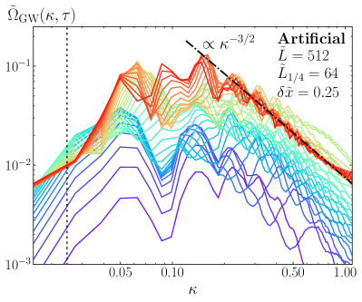
Figure 3: GW energy density spectrum of an artificial loop generated with $v_{1}=0.6$, $v_{2}=0.7$ and $\sin\alpha=0.5$. Each line corresponds to a different time, going from blue to red, and with separations of two units of program time. The vertical dotted line indicates the scale associated to the initial string length.

We first analyze lattice discretization effects on the GW spectrum of a loop. For network loops we run a high resolution simulation with $\delta\tilde{x}=0.125$ and $\tilde{L}=144$, and create new lattices with lower resolution, $\delta\tilde{x}^{(p)}=p\delta\tilde{x}$ ($p=2,3,4$), by eliminating $p-1$ sites (per dimension) of every $p$ consecutive points of the original lattice. For artificial loops we run simulations with different lattice spacing and fixed $\tilde{L}=192$, $\tilde{L}_{1/4}=96$ and initial parameters $v_{1}=0.7$, $v_{2}=0.6$, $\sin\alpha=0.5$. Figs. 2-(A) and 2-(B) show the evolution of the GW spectrum for these network and artificial loops, respectively. In all cases GW emission peaks at IR scales $\kappa\sim(2-6)\kappa_{0}$, with $\kappa_{0}=2\pi/\tilde{L}_{0}$ the scale of the initial string length $\tilde{L}_{0}$, and there is always good agreement between spectra up to a scale $\kappa_{\rm cut}\simeq 0.1\kappa_{\text{c}}$ for different $\delta\tilde{x}$, with $\kappa_{\text{c}}\equiv 2\pi/\tilde{r}_{\text{c}}$ the scale of the core radius. A second peak emerges at higher modes, but its height is suppressed as the UV resolution is improved, effectively disappearing for the smallest $\delta\tilde{x}$ in both types of loops. This second peak is therefore a lattice artifact arising when the string core is not well resolved. We thus compute the total energy emitted in GWs by integrating the spectrum up to the cut-off scale $\kappa_{\rm cut}$, guaranteeing in this way that the result is independent of the resolution $\delta\tilde{x}$. Finally, we note that the GW power is completely suppressed for length scales smaller than the core radius, $\kappa>\kappa_{\text{c}}$ (black dashed lines Fig. 2).

We also study the effect of varying the IR coverage in the case of artificial loops. Fixing $\delta\tilde{x}=0.25$, $v_{1}=0.6$, $v_{2}=0.7$, $\sin\alpha=0.5$, and $\tilde{L}_{1/4}=64$, we vary the ratio $\tilde{L}/\tilde{L}_{1/4}$. The resulting GW spectra are shown in Fig. 2-(C), multiplied by a factor to account for lattice-size dependencies. While large discrepancies are observed for the smallest box, the spectra converge as the box size increases. GW emission is suppressed for scales larger than the initial loop length $\kappa<\kappa_{0}$ (black dotted line). A zoomed-in version of the spectra from the largest box is found in Fig. 3, where we note the presence of various peaks in the spectrum. Although the peak structure resembles the harmonic pattern of GW emission expected in NG strings, the peak frequencies here are not in harmonic proportions, and their absolute and relative location actually varies between early (blue) and late (red) times. We note that the high-frequency tail of the spectrum approximately scales as $\propto k^{-3/2}$ (dot-dahsed line), which represents a steeper fall than the standard NG tail $\propto k^{-4/3}$ for cusp-dominated GW emission.

We finally determine a (rolling average) measurement of the total GW power emitted by a loop as

$$P_{\rm GW}(t)\equiv\frac{L^{3}\rho_{\varphi}}{2T}\int^{t+T}_{t-T}\text{d}t^{\prime}\int_{0}^{k_{\text{cut}}}\dot{\Omega}_{\text{GW}}(k,t^{\prime})\,\text{d}\log k\,,$$ (5)

which in terms of program variables can be written as $\tilde{P}_{\rm GW}=(P_{\rm GW}/v^{2})\,/\,(v/m_{\text{p}})^{2}$. This is shown in Fig. 4 for $\tilde{T}\equiv T/\sqrt{\lambda}v=15$ and UV cutoff $\kappa_{\text{cut}}=1$, chosen to prevent capturing the artificial UV-peak. The upper panel corresponds to network loops of different initial length $\tilde{L}_{0}$, simulated in lattices with varying $\tilde{L}$ and $\delta\tilde{x}$. We observe that in all cases the GW power emitted does not depend on $\tilde{L}_{0}$ and is roughly constant in time (though the exact time evolution of $\tilde{P}_{\rm GW}$ depends on the specific details of the collapse dynamics of each loop). At late times $\tilde{P}_{\rm GW}$ simply drops off as the loops finally disappear. Remarkably, there is no evidence of any systematic variation of the GW power emitted due to the shrinking of the loops. Between $\tau=30-100$, the average emission of all loops is of the order $\tilde{P}_{\rm GW}=240\pm 80$ (grey dashed line and band). Although there is no a priori reason to expect this to be similar to the NG prediction, $P_{\text{NG}}=(\Gamma/8\pi)\mu^{2}/m_{\text{p}}^{2}$, it is still instructive to make the comparison. Using $\mu=\pi v^{2}$ and $\mathit{\Gamma}=50$ [49], one gets $\tilde{P}_{\text{NG}}=\pi\mathit{\Gamma}/8\approx 20$, which is roughly an order of magnitude smaller than our result.

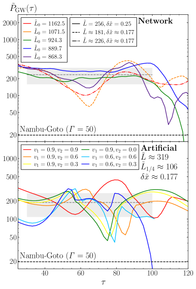
Figure 4: Rolling-averaged GW power emitted by network loops of different length (top) and artificial loops with distinct boost velocities (bottom), computed using eq. 5 with $\tilde{T}=15$ ad $\kappa_{\text{cut}}=1$.

Results for artificial loops with different boost velocities are presented in the lower panel of Fig. 4. All simulations are performed in boxes of $\tilde{L}=450/\sqrt{2}\approx 319$ and $\delta\tilde{x}=0.25/\sqrt{2}\approx 0.177$, with initial string separation $\tilde{L}_{1/4}=\tilde{L}/3$, chosen to reduce IR effects. For all pairs $\{v_{1},v_{2}\}$, hence for all choices of $\tilde{J}_{0}$, the GW power emission is of a similar order as for network loops, again with an amplitude that does not show large variations as the loops shrink. Fluctuations are however observed, which we believe are in part related to superposition of different GW fronts arising from the very peculiar symmetry of the squared configuration of the loops. Between $\tau=30-100$ the average emission of all loops is of the order $\tilde{P}_{\rm GW}=190\pm 80$ (grey dashed line and band), once again an order of magnitude larger than the NG result.

Comparing the GW and particle emission rates for both types of loop leads to

$${P_{\rm GW}\over P_{\varphi}}\approx\left\{\begin{array}[]{ll}\displaystyle{(240\pm 80)\over(14.2\pm 2.6)}\left({v\over m_{\text{p}}}\right)^{2}\,,&{\rm Network~{}loops,\vspace*{1mm}}\\ \displaystyle{(190\pm 80)\over(5.2\pm 2.5)}\left({v\over m_{\text{p}}}\right)^{2}\,,&{\rm Artificial~{}loops,}\end{array}\right.$$ (8)

where $P_{\varphi}$ for artificial loops is taken as an average over all families considered in Table 1. As the string scale cannot be arbitrarily large, e.g. CMB constraints require $v/m_{\text{p}}\lesssim 10^{-6}$ [50], we conclude that ${P_{\rm GW}/P_{\varphi}}\ll 1$, indicating that loop decay into GWs is completely sub-dominant compared to particle emission. This actually justifies a posteriori our assumption that backreaction of GW emission onto the loop dynamics could be neglected.

Discussion.– In this Letter, we have studied the decay of global string loops into GWs and scalar particles. Our results show that the latter totally dominates the decay of every type of loop we have considered, independent of their shape and initial condition (length, angular momentum, energy, etc), with a universal suppression of GW to particle emission by ${P_{\rm GW}/P_{\varphi}}\simeq\mathcal{O}(10)(v/m_{\text{p}})^{2}\ll 1$ for any acceptable $vev$ $v$. This constitutes the main result of our work. Our lattice study shows that the above conclusion is robust for a separation of scales ranging a factor $\sim 80-1700$ between the initial length of a loop and its core width, with no indication that this would change if the separation of such scales is increased further.

Extrapolating our results to cosmological scales might provide a new strategy to calculate the GWB spectrum from a global string network. While current attempts are based on lattice simulations of entire networks [51, 52, 53], or on a mixture of field theory and NG ingredients put together [54, 55], one should be able to obtain the GWB spectrum from a convolution of the loop number density at cosmological scales [56, 57, 58] with our newly calibrated GW power emission. The advantage of this method is that we have determined the GW emission of individual loops without having to resolve at the same time the separation $d_{\text{s}}$ between strings in the network, and without losing resolution of the string core as field evolution progresses. Taking into account that the GW power emission we obtain is independent of the string length and it scales as $\propto v^{2}(v/m_{\text{p}})^{2}$, and not proportional to a logarithmically growing tension as $\propto v^{2}(v/m_{\text{p}})^{2}\log^{2}(d_{\text{s}}/r_{\text{c}})$, together with the fact that global string loops are short lived, we anticipate that our results are expected to greatly suppress the overall amplitude of the GWB from cosmic string networks. We will present the details of this in a separate publication.

Supplemental material

Figure S1: Three-dimensional snapshots of $|\varphi|^{2}=0.1v^{2}$ surfaces from a network simulation with $\tilde{L}=64$ and $\delta\tilde{x}=0.25$. The snapshots correspond to the end of diffusion at $\tau=\tau_{0}=70$ (left), the end of the extra-fattening phase at $\tau=84.5$ (center), and the detection of a single isolated loop at $\tau=96$ (right).

Generation of isolated network loops. Network loops originate from the decay of string networks which are close to the scaling regime [42, 43, 44]. These networks are generated following the procedure detailed in [35]. Namely, we start simulations with a realization of a random Gaussian field $\varphi=(\phi_{1}+i\phi_{2})/\sqrt{2}$ in Fourier space, with power spectrum for each field component

$$\mathcal{P}_{\phi_{i}}(k)=\frac{k^{3}v^{2}\ell_{\text{str}}^{3}}{\sqrt{2\pi}}\exp\left(-\frac{1}{2}k^{2}\ell_{\text{str}}^{2}\right)\,,\quad i=1,~{}2\,,$$ (9)

normalized such that $\langle\phi_{1}^{2}+\phi_{2}^{2}\rangle=v^{2}$, where $\langle\cdots\rangle$ denotes expectation value. Here $\ell_{\text{str}}$ is a correlation length that controls the string density of the resulting network. This resulting field configuration is initially too energetic, so we remove the excess energy by evolving the configuration through out a diffusion process, modeled via the equation

$$\dot{\phi}_{i}-\nabla^{2}\phi_{i}=-\lambda\left(\phi_{1}^{2}+\phi_{2}^{2}-v^{2}\right)\phi_{i}\,,\quad i=1,~{}2\,.$$ (10)

We diffuse the field for 20 units of program time, which is enough to leave a smooth string configuration. An example of the resulting string network is represented in the first panel of Fig. S1

Following, the string network is evolved in a radiation-dominated background, with equation of motion

$$\ddot{\phi}_{i}+2\frac{\dot{a}}{a}\dot{\phi}_{i}-\nabla^{2}\phi_{i}=-a^{2}\lambda\left(\phi_{1}^{2}+\phi_{2}^{2}-v^{2}\right)\phi_{i}\,,\quad i=1,~{}2\,,$$ (11)

where $a=t/t_{0}$, $t$ denotes the conformal time, $t_{0}$ is its time when evolution begins and $\dot{f}=\text{d}f/\text{d}t$. In our simulations, we use $t_{0}=70/\sqrt{\lambda}v$. The background expansion is maintained for a half-light-crossing time of the lattice, $\Delta t_{\text{HL}}=L/2$. To avoid losing resolution of the string cores due to the expansion of the universe, the string-core resolution-preserving approach from [41] is adopted, also known as extra-fattening, in which the coupling parameter is promoted to a time-dependent constant, $\lambda\rightarrow a^{4}\lambda$. The extra-fattening lasts for a time $\Delta t_{\text{ef}}=\sqrt{t_{0}(t_{0}+\Delta t_{\text{HL}})}$, so that at time $t_{0}+\Delta t_{\text{HL}}$ the string-core width is equal to the initial one. The second panel of Fig. S1 shows an example of the network at the end of the extra-fattening phase.

At this point, networks are close to the scaling regime, with the mean string separation growing almost linearly with conformal time and the mean square velocity being constant, but the networks have not yet decayed into an isolated loop. The field is then evolved in a Minkowski background ($a(t)=1,\dot{a}=0$) for a maximum time of $\Delta t_{\text{HL}}/2$, which we found to be enough for the networks to decay into a single loop. An example of such loop is shown in the last panel of Fig. S1. We have found that $\sim 35\%$ of the simulations have decayed into single loops after this time, with the remaining forming multiple loops or infinite strings, and hence not being suitable for our study.

After finding an isolated loop, we turn on the emission of gravitational waves and study the evolution of the loop, still in Minkowski space-time, until it completely decays. Only $\sim 40\%$ of the isolated loops could be used for this study. We discarded those for which the loop self-intersected creating infinite strings, attracted itself around the box preventing its decay, or was much longer than the box size.

Figure S2: Schematic representation of the relevant variables used for the creation of a pair of parallel strings (left) and for isolating the inner loop (right). In the left panel, $b$ has been exaggerated compared to the actual simulations, which use $r_{\text{c}}\lesssim b\ll a=L_{1/4}/2$. In the right panel, red and blue regions are substituted by a smooth field configuration in two separate steps of the isolation procedure.

Generation of isolated artificial loops. Artificial loops are generated from the intersection of two pairs of boosted parallel infinite strings following [33]. We consider lattice coordinates varying from 0 to $L$, where $L$ is the lattice side, and take the pairs to be parallel to the $z$ and $x$ axis, respectively. Quantities associated to each of these pairs will be denotes with a “1” and “2” subscript, in this same order.

We first describe how the pair parallel to the $z$ axis is produced. To generate each of the strings, we consider the Nielsen-Olsen (NO) vortex solution for an infinite string, $\varphi_{\text{NO}}^{\pm}(x,y)=f(r)~{}\text{exp}(\pm i\theta)/\sqrt{2}$, where $(r,\theta)$ are cylindrical coordinates around the $z$-axis and $f(r)$ is a numeric function. The string solution is boosted with velocity ${\vec{v}}=v_{1}(\sin\alpha_{1},\cos\alpha_{1})$ in the $(x,y)$-plane, $\varphi_{{\vec{v}}_{1}}^{\pm}(x,y,t)=\varphi_{\text{NO}}^{\pm}(x^{\prime},y^{\prime})$, where

$$\begin{array}[]{lr}x^{\prime}&=-\gamma_{1}v_{1}st+[1+(\gamma_{1}-1)s_{1}^{2}]x+(\gamma_{1}-1)s_{1}c_{1}y\,,\\ y^{\prime}&=-\gamma_{1}v_{1}ct+(\gamma_{1}-1)s_{1}c_{1}x+[1+(\gamma_{1}-1)c^{2}]y)\,,\end{array}\quad\quad\text{with}\quad\quad c_{1}=\cos\alpha_{1}\,,s_{1}=\sin\alpha_{1}\,,\gamma_{1}=(1-v_{1}^{2})^{1/2}\,.$$ (12)

This allows to obtain the field and its time-derivative. A pair of strings parallel to the $z$ axis is then constructed using the product ansatz [33] on two displaced boosted strings,

$$\varphi_{1}(x,y,t)=\frac{1}{v}\varphi_{{\bf v}_{1}}^{+}\left(x-\left(\frac{L}{2}+a_{1}\right),y-\left(\frac{L}{2}+b_{1}\right),t\right)\varphi_{-{\bf v}_{1}}^{-}\left(x-\left(\frac{L}{2}-a_{1}\right),y-\left(\frac{L}{2}-b_{1}\right),t\right)\,.$$ (13)

The variables used for the construction of one pair of strings are schematically represented in the left panel of fig. S2. Note that in this work we consider equal velocities and displacements for both strings of each pair.

The resulting configuration and its derivative, evaluated at $t=0$, are modified following [33] to incorporate them in a periodic lattice. Finally we note that the product ansatz is used twice so that the initial configuration is obtained by multiplying two pairs parallel to the $z$ and $x$ axis, $\varphi(x,y,z)=\varphi_{1}(x,y,0)\varphi_{2}(z,y,0)/v$. An example of the resulting field is shown in the first panel of Fig. S3.

In this work, we consider the two-string pairs to have, in general, different velocity magnitudes, $v_{1}\neq v_{2}$ with $v_{2}\geq v_{1}$, but the same angle with respect to the normal to the plane where the strings intersect, $\alpha_{1}=\alpha_{2}$. We also consider all strings to initially lie almost in that same plane. We let $a_{1}=-a_{2}$ be a significant fraction of the lattice size, typically $L/4$ or $L/6$, while $b_{1}=0$ and $b_{2}=2/\sqrt{\lambda}v$. This choice ensures strings to be separated enough so that the product ansatz remains valid, and that the two pairs are close enough so the intersection happens very early in the simulation. The (approximmate) separation of two parallel strings is denoted $L_{1/4}=2a$, so that the initial length $L_{0}$ of the loops is of the order of $4L_{1/4}$.

The initial configuration is evolved using eq. (11) in a flat background ($a(t)=1,\dot{a}=0$), and the four straight strings rapidly intersect forming two squared loops, one inner and one outer. Shortly after, the two loops start to shrink and separate from each other. We have developed a procedure to isolate the inner loop at this point, as we expect such loop to be less affected by the initial conditions than the outer loop. The procedure is based on the fact that both loops are almost planar and the center of the inner loop is close to the center of the box. This procedure is schematically represented in the right panel of Fig. S2.

Figure S3: Three-dimensional snapshots of the $|\varphi|^{2}=0.06v^{2}$ surfaces from an artificial loop simulation with initial conditions $v_{1}=0.8,v_{2}=0.6,\sin\alpha=0.5$ and $L_{1/4}=L/2$, and simulation parameters $\tilde{L}=64$ and $\delta\tilde{x}=0.25$. The snapshots correspond to the start of the simulation at $\tau=0$ (left), and to times immediately before (center) and after (right) the application of the isolation procedure at $\tau=2.5$.

After formation, we let the loops evolve until their separation is a fraction (typically a factor $0.15$) of the radius of the central one. At this point, we consider a cylinder with its axis along the $y$ axis and radius $R$, such that it encompasses the inner loop and its surface lies halfway between the two loops. The field outside of the cylinder and its time derivative are then substituted with a smooth configuration containing no string. The substitution is performed in two steps, repeated for each fixed value of the coordinate $y=y_{\star}$. First, one considers those points $(x,y_{\star},z)$ outside the cylinder with $|L/2-x|<R$ (red area in the right panel of Fig. S2). Each possible value of $x=x_{\star}$ defines a one-dimensional surface that intersects the cylinder at $z_{1}$ and $z_{2}>z_{1}$. The field and its conjugate momentum outside the cylinder in this line are then substituted with a smooth configuration. The phases are linearly interpolated using the phase values at $z_{1,2}$, while for the field modulus an ansatz based on the long-distance behavior of the NO solution is used. For the field we have,

$$|\varphi(x_{\star},y_{\star},z)|=\left\{\begin{array}[]{lr}\displaystyle\frac{A_{1}}{(\Delta-z+z_{1})^{2}}+\frac{A_{2}}{(L+z+\Delta-z_{2})^{2}}+\frac{v}{\sqrt{2}}\,,&\quad\quad\quad 0\leq z<z_{1}\,,\\ \displaystyle\frac{A_{1}}{(L-z+\Delta+z_{1})^{2}}+\frac{A_{2}}{(\Delta+z-z_{2})^{2}}+\frac{v}{\sqrt{2}}\,,&\quad\quad\quad z_{2}<z<L\,,\end{array}\right.$$ (14)

and for its derivative,

$$|\dot{\varphi}(x_{\star},y_{\star},z)|=\left\{\begin{array}[]{lr}\displaystyle\frac{B_{1}}{(\Delta-z+z_{1})^{3}}+\frac{B_{2}}{(L+z+\Delta-z_{2})^{3}}\,,&\quad\quad\quad 0\leq z<z_{1}\,,\\ \displaystyle\frac{B_{1}}{(L-z+\Delta+z_{1})^{3}}+\frac{B_{2}}{(\Delta+z-z_{2})^{3}}\,,&\quad\quad\quad z_{2}<z<L\,,\end{array}\right.$$ (15)

where $A_{1,2}$ and $B_{1,2}$ are normalization constants that ensure the configuration is periodic and match in the surface of the cylinder, and $\Delta$ is a length parameter we set to $\Delta=2/\sqrt{\lambda}v$. In a second step, we consider points with $|L/2-x|\geq R$, and proceed analogously working with fixed $z=z_{\star}$ (blue regions in the right panel of Fig. S2). Both steps are finally repeated for all values of $y_{\star}$. The central and right panels of Fig. S3 show an example of a field configuration just before and after isolating the inner loop. After the isolation procedure is complete, we turn on gravitational waves and study the loop until it completely decays.

We have checked the effect of varying $\Delta$, as well as the isolation time and the size of the cylinder, finding that the results are insensitive to these changes as long as $a)$ both strings are sufficiently separated away, and $b)$ the cylinder surface is not too close to any of the two loops.

Spectra of massless and massive modes. The broken phase of the model in Eq. (1) is characterized by the presence of massless ($\theta$) and massive ($\chi$) field excitations. These correspond, respectively, to angular and radial perturbations from the true vacuum of the theory, $\varphi=\frac{v+\chi}{\sqrt{2}}\exp(i\theta)$. In Fig. S4 we plot power spectra of $\chi$ (left) and $\theta$ (right) at the end of the decay of an artificial loop generated with $v_{1}=v_{2}=0.6$, $\sin\alpha=0.4$ and $L_{1/4}=L/2$. For a generic field $\phi$, the power spectrum is defined as $\Delta_{\phi}(k)=k^{3}|\phi(k)|^{2}/2\pi^{2}$, with $\phi(k)$ the Fourier transform of $\phi$. In program variables, we have $\tilde{\theta}=\theta$, $\tilde{\chi}=\chi/v$ and $\tilde{\Delta}_{\tilde{\phi}}(\kappa)=\lambda v^{5}\Delta_{\phi}(k)$. We note how the spectrum of the massless field is suppressed at high modes, while the spectrum of the massive field peaks around $\kappa\sim 1$.

Figure S4: Power spectra of massless (left) and massive (right) particles just after the decay of an artificial loop with $v_{1}=v_{2}=0.6$ and $\sin\alpha=0.4$. Dashed vertical lines indicate the scale of the string width, $\kappa_{\text{c}}=2\pi/\tilde{r}_{\text{c}}\simeq 9$.

In [33], the energy power spectrum per linear interval for these two modes was determined for artificial loops with these same initial conditions, and the authors showed the appearance of a peak in the energy spectrum of $\theta$. In Fig. S5, we present in red our results for the energy spectrum of the massless field after the loop decay, which for small perturbations is defined as

$$E_{\theta}(k)=\frac{v^{2}}{2}\left[|\dot{\theta}({\vec{k}})|^{2}+k^{2}|\theta({\vec{k}})|^{2}\right]\,.$$ (16)

We observe the same scaling of the spectrum with $\propto k^{-1}$ as in [33], but we detect no presence of a sharp peak. Interestingly, if we set the initial radius of the string to be larger than the physical one by modifying the NO vortex solution as $f(r)\rightarrow f(2r)$, we observe a peak appearing at the same scale scale as in [33]. (Note we find the peak at $\kappa=k/\sqrt{\lambda}v\approx 1/\sqrt{2}$, and in [33] the values $v=1$, $\lambda=1/2$ are used). In our case it looks like if this peak is related to an excess energy in the radial mode of the string due to an excessively large core width of the initial strings. Furthermore, we only observe ’bulges’ in the three-dimensional representation of the field, as those discussed in [33], when considering this extra large initial radius.

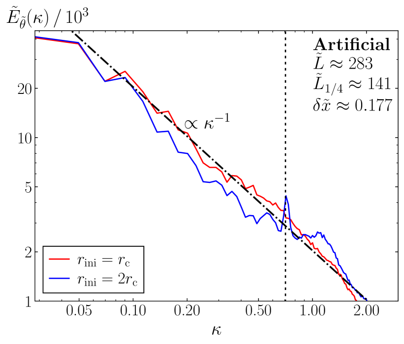
Figure S5: Energy power spectrum per linear interval of massless radiation at the end of the decay of an artificial loop initialized with $v_{1}=v_{2}=0.6,\sin\alpha=0.4$ and $L_{1/4}=L/2$, both in the case of initial core radius, $r_{\text{ini}}$ equal to the physical one (red) and twice as big (blue). We observe the same scaling as in [33], but only find the sharp peak for the physically unrealistic initial conditions.

Simulation parameters. This section summarizes the parameters used in our simulations run to study the loop dynamics. Table 2 refers to network loops, characterized by $\{\tilde{L},\delta\tilde{x},\tilde{\ell}_{\text{str}}\}$, while Table 3 presents the initial conditions and simulation parameters used for artificial loops. Note that for each of the 7 families of initial conditions, a simulation is performed for all sets of $\{\tilde{L},\tilde{L}_{1/4},\delta\tilde{x}\}$.

$\tilde{L}$	$\delta\tilde{x}$	$\tilde{\ell}_{\text{str}}$	$\tilde{L}_{0}$
256	0.25	25	868.3
256	0.25	20	924.3
256	0.25	20	889.7
$320/\sqrt{2}\approx 226.3$	$0.25/\sqrt{2}\approx 0.177$	22	1162.48
$256/\sqrt{2}\approx 181.0$	$0.25/\sqrt{2}\approx 0.177$	15	1071.5
$256/\sqrt{2}\approx 181.0$	$0.25/\sqrt{2}\approx 0.177$	15	684.0
$256/\sqrt{2}\approx 181.0$	$0.25/\sqrt{2}\approx 0.177$	15	371.2
144	0.25	12	557.0
144	0.25	12	296.3
144	0.1875	12	605.0
144	0.1875	12	553.5
144	0.125	12	633.6
$192/\sqrt{2}\approx 135.8$	$0.25/\sqrt{2}\approx 0.177$	15	728.6
$192/\sqrt{2}\approx 135.8$	$0.25/\sqrt{2}\approx 0.177$	15	699.8
$192/\sqrt{2}\approx 135.8$	$0.25/\sqrt{2}\approx 0.177$	15	582.2
$192/\sqrt{2}\approx 135.8$	$0.25/\sqrt{2}\approx 0.177$	15	462.4
$192/\sqrt{2}\approx 135.8$	$0.25/\sqrt{2}\approx 0.177$	15	405.2
128	0.25	10	433.2
$128/\sqrt{2}\approx 90.5$	$0.25/\sqrt{2}\approx 0.177$	8	260.7
$128/\sqrt{2}\approx 90.5$	$0.25/\sqrt{2}\approx 0.177$	8	234.1
$128/\sqrt{2}\approx 90.5$	$0.25/\sqrt{2}\approx 0.177$	8	215.2
$128/\sqrt{2}\approx 90.5$	$0.25/\sqrt{2}\approx 0.177$	8	88.2
$128/\sqrt{2}\approx 90.5$	$0.25/\sqrt{2}\approx 0.177$	8	60.3

Table 2: Summary of the simulation parameters used to study the decay of network loops, together with the initial length of the isolated loops estimated from the number of pierced plaquettes taking the Manhattan effect into account.

$v_{1}$	$v_{2}$	$\sin\alpha$
0.9	0.9	0.4
0.9	0.6	0.4
0.9	0.3	0.4
0.9	0.0	0.4
0.6	0.6	0.4
0.6	0.3	0.4
0.3	0.3	0.4

$\tilde{L}$	$\tilde{L}_{1/4}$	$\delta\tilde{x}$
$50/\sqrt{2}\approx 35.4$	$25/\sqrt{2}\approx 17.7$	$0.25/\sqrt{2}\approx 0.177$
$100/\sqrt{2}\approx 70.7$	$50/\sqrt{2}\approx 35.4$	$0.25/\sqrt{2}\approx 0.177$
$150/\sqrt{2}\approx 106.1$	$75/\sqrt{2}\approx 53.0$	$0.25/\sqrt{2}\approx 0.177$
$200/\sqrt{2}\approx 141.4$	$100/\sqrt{2}\approx 70.7$	$0.25/\sqrt{2}\approx 0.177$
$250/\sqrt{2}\approx 176.8$	$125/\sqrt{2}\approx 88.4$	$0.25/\sqrt{2}\approx 0.177$
$300/\sqrt{2}\approx 212.1$	$150/\sqrt{2}\approx 106.1$	$0.25/\sqrt{2}\approx 0.177$
$400/\sqrt{2}\approx 282.8$	$200/\sqrt{2}\approx 141.4$	$0.25/\sqrt{2}\approx 0.177$

Table 3: Summary of the initial conditions (left) and simulation parameters (right) used to study the decay of artificial loops. For each family of initial conditions, a simulation is performed using each $\{\tilde{L},\tilde{L}_{1/4},\delta\tilde{x}\}$ set.