Detection of Binary Black Hole Mergers from the Signal-to-Noise Ratio Time Series Using Deep Learning
Abstract
Gravitational wave detection has opened up new avenues for exploring and understanding some of the fundamental principles of the universe. The optimal method for detecting modelled gravitational-wave events involves template-based matched filtering and doing a multi-detector search in the resulting signal-to-noise ratio time series. In recent years, advancements in machine learning and deep learning have led to a flurry of research into using these techniques to replace matched filtering searches and for efficient and robust parameter estimation. This paper presents a novel approach that utilizes deep learning techniques to detect gravitational waves from the signal-to-noise ratio time series produced from matched filtering. We do this to investigate if an efficient deep-learning model could replace the computationally expensive post-processing in current search pipelines. We present a feasibility study where we look to detect gravitational waves from binary black hole mergers in simulated stationary Gaussian noise from the LIGO detector in Hanford, Washington. We show that our model can match the performance of a single-detector matched filtering search and that the ranking statistic from the output of our model was robust over unseen noise, exhibiting promising results for practical online implementation in the future. We discuss the possible implications of this work and its future applications to gravitational-wave detection.
I Introduction
Gravitational waves (GWs) were first detected by the Laser Interferometer Gravitational-Wave Observatory (LIGO) Aasi et al. (2015) on September 14, 2015 Abbott et al. (2016). Since then, 90 GW events from compact-binary-coalescences (CBCs) have been detected across three separate observing runs Abbott et al. (2019, 2021a, 2021b, 2021c) by the LIGO and Virgo Acernese et al. (2015) detectors. With upgrades to these existing detectors improving their sensitivity, and additional detectors such as the Kamioka Gravitational Wave Detector (KAGRA) Akutsu et al. (2021) and LIGO-India Saleem et al. (2022) coming online, the opportunity to detect new GW events is increasing dramatically in each observing run. Therefore, it is becoming more prevalent to develop efficient search algorithms for the future of gravitational-wave astronomy.
Currently, four approved search pipelines search for modelled gravitational-wave events from the strain of the GW detectors, including PyCBC Live Nitz et al. (2018); Dal Canton et al. (2021), GstLAL Cannon et al. (2020), SPIIR Chu et al. (2022) and MBTA Aubin et al. (2021). These pipelines are all based on the technique of matched filtering, which employs a comprehensive bank of modelled GW waveform templates to perform a cross-correlation with the detector strain data to identify matching signals. When the match between the template and data achieves a predefined threshold and the data passes the data quality checks, an event trigger can be produced. Matched filtering search pipelines are inherently computationally expensive, resulting in minimum detection latencies of Chu et al. (2022); Dal Canton et al. (2021), with additional latency for parameter estimation used to localize and classify the sources. To most efficiently detect GW events, search pipelines need to minimize detection latency and maximize the robustness of each detection.
Deep learning LeCun et al. (2015); Krizhevsky et al. (2012); Simonyan and Zisserman (2015); Goodfellow et al. (2016) is a subset of machine learning that uses artificial neural network models to make predictions by extracting features from input data for problems such as classification and regression. In recent years, deep learning has been applied to gravitational-wave physics for problems such as binary black hole (BBH) merger detection George and Huerta (2018a, b); Huerta et al. (2021); Gabbard et al. (2018); Fan et al. (2019); Rebei et al. (2019); Gebhard et al. (2019); Santos et al. (2022); Corizzo et al. (2020); Lin and Wu (2021); Deighan et al. (2020); Wei et al. (2021); Xia et al. (2021); Schäfer et al. (2022); Schäfer and Nitz (2022); Verma et al. (2022a); Ma et al. (2022); Verma et al. (2022b); Andrews et al. (2022); Yan et al. (2022); Barone et al. (2022); Schäfer et al. (2023); Nousi et al. (2023); Morales et al. (2021); Kim et al. (2021, 2022); Álvares et al. (2020); Menéndez-Vázquez et al. (2021); Fan et al. (2021); Lopac et al. (2022); Ravichandran et al. (2023); Andres-Carcasona et al. (2023); Jadhav et al. (2021, 2023); Wang et al. (2020); Jiang et al. (2022); Bresten and Jung (2019) and parameter estimation Fan et al. (2019); Álvares et al. (2020); Chatterjee et al. (2019); McLeod et al. (2022); Chatterjee et al. (2022); Chatterjee and Wen (2022); Dax et al. (2021), and it has been shown that these models are capable of enabling and accelerating these computationally expensive problems. One of the main motivations for implementing deep learning for these tasks is that the computationally expensive training process can be done offline. This allows for rapid inference in real-time, where current algorithms may take hours or even days.
Previous research on detecting gravitational waves with deep learning has mostly looked at making detections from the detector strain data George and Huerta (2018a, b); Huerta et al. (2021); Gabbard et al. (2018); Fan et al. (2019); Rebei et al. (2019); Gebhard et al. (2019); Santos et al. (2022); Corizzo et al. (2020); Lin and Wu (2021); Deighan et al. (2020); Wei et al. (2021); Xia et al. (2021); Schäfer et al. (2022); Schäfer and Nitz (2022); Verma et al. (2022a); Ma et al. (2022); Verma et al. (2022b); Andrews et al. (2022); Yan et al. (2022); Barone et al. (2022); Schäfer et al. (2023); Nousi et al. (2023) or time-frequency spectrograms Morales et al. (2021); Kim et al. (2021, 2022); Álvares et al. (2020); Menéndez-Vázquez et al. (2021); Fan et al. (2021); Lopac et al. (2022); Ravichandran et al. (2023); Andres-Carcasona et al. (2023); Jadhav et al. (2021, 2023). Detecting CBC mergers from these data sources using deep learning becomes difficult when looking at lower mass events such as binary neutron star (BNS) and neutron star-black hole (NSBH) mergers. This is because as the signal duration increases for lower mass binaries, the signal power is spread over a longer period, and the signal has a lower overall amplitude. There have also been publications that use the peak values of the signal-to-noise ratio (SNR) time series produced by matched filtering as the input to a deep learning model, with template sets consisting of 35 Wang et al. (2020) and 57 Jiang et al. (2022) template waveforms.
This paper presents a unique approach for detecting gravitational waves from spinning binary black hole mergers by using the SNR time series produced by matched filtering as the input to our deep learning model. This is advantageous in several aspects, including that the SNR time series is readily available from online and offline search pipelines and that the SNR time series projects all of the signal power into a small time window. This is consistent for all CBC source types, meaning our deep learning model can be easily adapted for detecting BNS and NSBH events. Additionally, matched filtering is considered the optimal search method for identifying modelled signals in stationary Gaussian noise Wainstein et al. (1962). With a Gaussian noise background, comparing the detection performance of matched filtering with our deep learning model is a good feasibility study for implementing deep learning in detecting gravitational wave events in real noise where the background is non-stationary.
We have trained and tested a Residual Neural Network (ResNet) He et al. (2015) deep learning model, with an architecture that includes Convolutional Neural Network (CNN) Lecun et al. (1998) layers, Long Short-term Memory (LSTM) Hochreiter and Schmidhuber (1997) layers and Dense fully-connected layers Priddy and Keller (2005). CNNs, and ResNet models, are commonly used for image and pattern recognition tasks Simard et al. (2003); Krizhevsky et al. (2012) and are regularly used in various applications where feature recognition is required. LSTM networks are regularly used in time series prediction tasks Sak et al. (2014), as they can process time series data while remembering information about earlier segments.
We demonstrate the performance of our method through a feasibility study for the detection of BBH mergers in single-detector Gaussian noise. The result of this method is comparable with that of matched filtering. This is the first time deep learning has been applied to successfully detect gravitational waves from the SNR time series produced by matched filtering.
Section II discusses the methods we have used to train and test our deep learning model, including the process of matched filtering, the architecture of our deep learning model, and the datasets we have generated. Section III presents the results of our testing methods on our deep learning model and demonstrates the feasibility of using our model to search for BBH signals. Lastly, Section IV summarizes our results and presents future applications of this work and further research that could be done in this area.
II Method
II.1 Matched Filtering
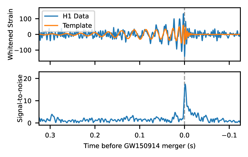
Since matched filtering is considered the optimal search method for identifying modelled signals in stationary noise, this is what the modelled gravitational wave search pipelines use to detect events. This means that the output SNR time series from matched filtering pipelines is a readily available dataset for us to integrate with. One of the main reasons we employ this method is that detecting events in the detector strain can be difficult for longer-duration merger signals as the power will be distributed over a more extended period. The benefit of the SNR time series is that the entire signal response is projected within a window of duration milliseconds for all CBCs in the current GW detectors’ sensitivity band. In addition to the constrained signal power, it also simplifies the complexity of our deep learning model, as we do not have to search for signals that vary significantly in duration as the source parameters change. Figure 1 illustrates the differences between the detector strain and the SNR time series produced by matched filtering for the first real detected BBH GW event, GW150914, with the template waveform having the same source parameters as estimated for the compact binary associated with the event.
Matched filtering is a technique that involves comparing the detector strain data , with a pre-defined template waveform . The template waveform is defined by its intrinsic source parameters , and GW search algorithms use template banks with hundreds of thousands of templates to cover the parameter ranges that are detectable from the GW detectors. This comparison is performed individually for each template waveform in the bank and is computed through a cross-correlation of the template with the strain data. The output of matched filtering is the SNR time series , which gives an estimate of the likelihood of a GW signal being present in the data, and is defined as Hooper (2013); Allen et al. (2012),
| (2) |
Here, is the Fourier transform of the detector strain data, is the Fourier transform of the template waveform, and is the PSD of the strain data. In Equation 1, is the normalization constant computed by the square root of the inner product of the template with itself, which is used to normalize the SNR time series.
II.2 Deep Learning Model
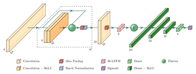
The output of matched filtering is the SNR time series, where gravitational wave signals can be identified by a sharp signal profile, and so we design a deep learning model to identify features of this type. Our detection model consists of a series of convolutional neural network layers with residual layers containing a skip connection, max-pooling, batch normalization layers Ioffe and Szegedy (2015), a bi-directional Schuster and Paliwal (1997) long short-term memory layer (LSTM), and a series of fully connected layers, some with dropout Srivastava et al. (2014). Our model was built, trained, and tested using the TensorFlow Abadi et al. (2015) package, and a detailed diagram showing the structure of the model can be found in Figure 2.
The input to our model is a 1-second SNR time series output from matched filtering of one template with the strain data. This time series is sampled at 2048 Hz, so our model input dimension is . In practice, our model would perform inference on the SNR time series from each template in a template bank separately, and the set of model outputs from doing this would be used to construct our detection ranking statistic. This exercise is beyond the scope of this research, as we investigated our model performance in a controlled test environment.
We implement convolutional neural network layers in our model as we are looking to identify the patterns produced by gravitational wave signals and disregard background noise. Residual neural networks implement a skip connection that allows a neural network to be trained with more layers and can prevent overfitting an overly complex model He et al. (2015). Since our input is the SNR time series data and we are trying to detect a well-defined signal profile, we also implement a bi-directional LSTM into our model. We use the bi-directional implementation of LSTMs instead of a uni-directional implementation as it processes the input matrix in the forward and backward directions, allowing for more robust signal identification. This was verified when designing our model, as the bi-directional LSTM design provided better performance for our model.
For the first three fully connected dense layers in our model, we implement a dropout of 0.1, meaning that at each step during training, 10% of the layers neurons will be randomly set to 0. This helps to prevent our model from overfitting during training but is not applied when the model is used for inference. We also use the Rectified Linear Unit (ReLU) activation function Nair and Hinton (2010) on the output of some of the convolution and dense layers, as it can handle the vanishing gradients problem and is extremely computationally efficient to compute. Our model output is two numbers indicating the probability that the sample contains pure noise or noise with a signal, and so we use the sigmoid layer to normalize these values such that they always sum to one. However, during testing, we replaced this sigmoid layer with a linear activation function so that our predictions are not rounded in the sigmoid layer based on the model’s float 32 precision. Replacing the sigmoid in this manner during testing was motivated by Schäfer et al. (2022). The new output value from this linear layer that indicates if the sample contains an injection is used as the ranking statistic for our model.
When training our model, we used the Adam optimizer Kingma and Ba (2014) with an initial learning rate of and a batch size of 1024, and we used the binary cross-entropy loss function. We utilized the ReduceLROnPlateau Keras Chollet et al. (2015) callback to reduce the learning rate by a factor of 10 during training when the validation accuracy hadn’t improved after three epochs. Additionally, we used the EarlyStopping callback from Keras to end the training process when the validation accuracy hadn’t improved after seven epochs, and this resulted in training taking 36 epochs and a training time of one hour on an NVIDIA P100 GPU.
II.3 Training Datasets
To generate training and testing data, a modified version of the sample generation code by Gebhard et al. Gebhard et al. (2019) is used. This code is modified to produce samples of strain and injections in just the LIGO Hanford (H1) detector, and we developed a module to generate matched filtering template banks and perform matched filtering with these templates on the generated strain data. The PyCBC package Nitz et al. (2022) is used to generate the background noise, the injection and template waveforms, and to perform matched filtering to get the SNR time series samples required to train and test our deep learning model.
To train and test our model, we require samples of pure noise and samples of noise with an injected signal. The noise segments are sampled from the advanced LIGO design sensitivity Power Spectral Density (PSD), aLIGOZeroDetHighPower, at a sampling frequency of 2048Hz. We generate our BBH injection and template waveforms using the SEOBNRv4 Bohé et al. (2017) waveform approximant.
To simulate our datasets’ injection and template waveforms, we first have to sample the source parameters from the ranges outlined in Table 1. For all sampled parameters in Table 1, except for declination, inclination angle, and SNR, we use a uniform prior over the ranges given. Source masses are measured in solar masses, , and we only investigate z-component spins relative to the orbital plane, . We uniformly sample the sine of the declination and the cosine of the inclination to have accurate astrophysical distributions. The SNR is sampled uniformly over the ranges 5 to 10, 10 to 20, 20 to 30, and 30 to 50, with each range contributing the same number of samples to the dataset. This sampling of the SNR gives a bias at lower SNR values where events are more likely to occur and where the performance of our model is more important. Since we are sampling in SNR, we are not required to sample the luminosity distance of the source, and we can instead simulate the waveforms at a fixed distance and rescale them to the correct signal power. We sample SNR instead of luminosity distance as we can more directly control the signal amplitudes in our training and testing data.
| Parameter | Minimum | Maximum |
|---|---|---|
| Source Masses () | 10 | 80 |
| Source Spins, | 0 | 0.998 |
| Coalescence Phase (rad) | 0 | 2 |
| Polarization Angle (rad) | 0 | 2 |
| Right Ascension (rad) | 0 | 2 |
| Declination (rad) | - | |
| Inclination Angle (rad) | 0 | |
| SNR | 5 | 50 |
To generate each strain sample, before passing it through matched filtering, we sample 16s of noise and inject a waveform if the sample is an injection sample, otherwise, we use it as a pure noise sample. Since matched filtering requires Fourier transforms to change between time and frequency domains, we position the injection merger in the centre of the sample and then cut out a section of the SNR time series around the injection to avoid any edge effects from the Fourier transforms in the final sample. For pure noise samples, we take the central 1-second of the SNR time series as our sample. When we trim each sample containing an injection, we take the 1-second sample such that the merger time is positioned randomly within the middle 0.6 seconds of the sample. This is so our model can learn to detect events across its viewing window.
We use a dataset of almost 140,000 SNR time series samples with injections to train our deep learning model. This comprises 5,400 unique injection waveforms, which we perform matched filtering on with 26 templates. These templates include 25 independent template waveforms randomly sampled from the same parameter space as the injections, and then for each injection sample, we use a template waveform with the same source parameters as the injection. We do this so that we are guaranteed to train our model on the ideal SNR time series response and with template waveforms without perfect overlap that can only recover a portion of the total signal power. We include the additional 25 templates because current LIGO search pipelines cannot exhaustively cover the detectable CBC parameter space due to the number of computational resources that would be required, meaning it is rare for search pipelines to see almost perfect matches of real events with templates. Additionally, our training dataset consists of 1,125,000 pure noise samples, which includes 45,000 unique noise strain samples, and uses the same set of 25 templates to produce the SNR time series samples. As it is important to train deep learning models on good generalizations of real-world data, our training dataset has a ratio of 8 to 1 pure noise to injection samples. We performed tests on different ratios of noise samples to injection samples for datasets of similar sizes but found this ratio gave our model the best trade-off between identifying samples as being noise or having an injection. During training, we combine our injection and pure noise datasets, shuffle them together, and then use 80% of the samples for training and 20% for validation.
II.4 Model Testing
To test the output of our deep learning model as a ranking statistic, we test it directly against a single-detector matched filtering search that uses the maximum SNR value of the sample as a ranking statistic, and we also analyze our statistic to show that it is robust for unseen test data. The first test is done by performing inference on 100,000 samples of pure noise and 100,000 injection samples and comparing the inference results between the two search methods. As in training, all samples have a duration of one second and are sampled at 2048Hz, and the injections are randomly positioned within the middle 0.6 seconds of the sample. We make three independent datasets of this size with injections with an SNR of four, six, or eight, where the injected waveform is a BBH waveform with primary and secondary component masses of 30 for all injection samples. Additionally, we use the injection waveform as the template for matched filtering to ensure a good signal response in the SNR time series. To infer our model sensitivity from the predictions on these datasets, we make thresholds across the range of output predictions of our model on the test datasets. At each of these thresholds, we can compute our model’s false alarm rate and detection efficiency (true alarm rate) to directly compare with a single-detector matched filtering search on a receiver-operating-characteristic curve.
The second test on our deep learning model is to show that the ranking statistic is robust in its predictions on unseen noise data. We do this by performing inference with our model on seconds (1 year) of Gaussian noise data and then on an independent seconds (1 week) dataset of Gaussian noise. By creating thresholds across the range of output values from our model after inference on the 1-year dataset, we can compute the number of samples with an output value higher than each threshold. The results of this allow us to define the false alarm rate assignment based on the output value of our model and can then be applied to the inference results of our model on the 1-week dataset. After assigning false alarm rates to the distribution of outputs from our model on the 1-week dataset, we can directly compare the number of events at each false alarm rate to that of the 1-year dataset. This is done by dividing the number of triggers from the 1-year dataset to accurately represent the expected number of triggers at each false alarm rate for a 1-week run. We do this to show that our false alarm rate assignment is consistent and applicable to unseen data. We use one template waveform for this test: a non-spinning binary black hole with 30 for the primary and secondary mass components. Using the measured inference times from the large-scale testing on the 1-year dataset, we have computed the computational resource requirements for real-time detection with a complete BBH template bank.
III Results
III.1 Detection Efficiency
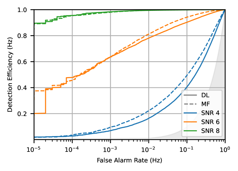
The sensitivity of our model can be seen in the receiver operating characteristic curve (ROC) of Figure 3. From the results of inference on the test datasets of each injection strength, we have computed the detection efficiency (true alarm rate) and false alarm rate at thresholds spaced throughout the range of prediction values. Since our sample duration is one second and there is no overlap between samples, the false alarm probability is equal to the false alarm rate. The false alarm rate is calculated as the number of noise samples with predictions above the threshold divided by the total number of pure noise samples. Similarly, the detection efficiency is computed as the number of injection samples with predictions above the threshold divided by the total number of injection samples.
Figure 3 presents this analysis for each of the three datasets with injections having an SNR of four, six, and eight, to directly compare our deep learning method with the single-detector matched filtering search mentioned in Section II.4. We stop at a maximum SNR of 8 because our model, and the matched filtering search, will have a detection efficiency of one within the range of the false alarm rates we can compute with the limited number of samples in the dataset. We see that our model is consistent in detection efficiency with the matched filtering search, especially at lower false alarm rates, where it is more important that our model can make confident detections. Results below a false alarm rate of Hz are jittery due to the number of samples approaching small numbers, so there can be a large amount of random variation, as seen for the SNR 6 line especially.
We find in Figure 3 that our model is slightly worse at recovering signals with an injection SNR of four. However, this is slightly outside our training parameter range for SNRs which is 5 to 50. Despite this, we see that the model has generalized quite well and can still perform consistently with the matched filtering search at lower false alarm rates. Making detections of events with an SNR of 4 in a single detector is expected to be rare, but it is important to test our model’s capabilities when our training set is designed for stronger events.
III.2 False Alarm Rate Evaluation
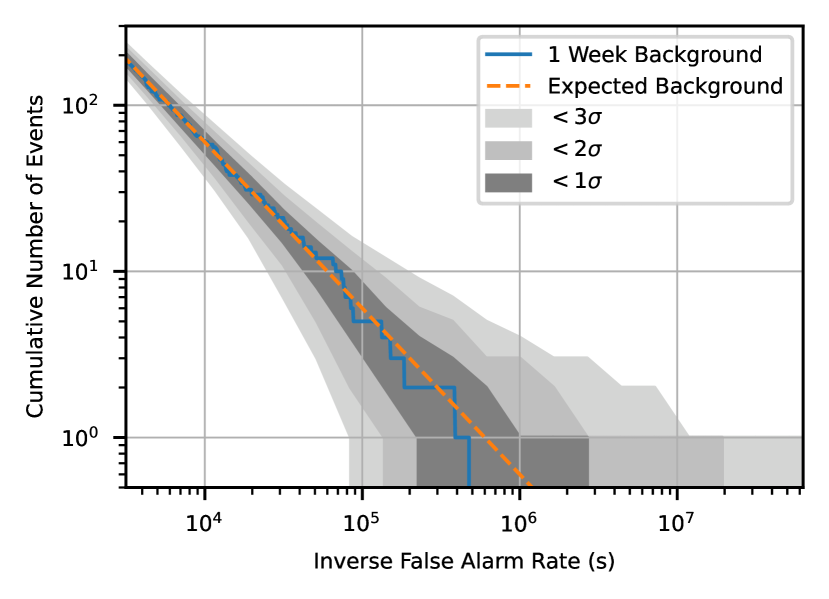
Figure 4 shows the cumulative number of samples with model outputs above each inverse false alarm rate threshold for each test dataset in our second testing method. We find that there is very good agreement between the expected 1-week background trigger counts and the actual 1-week background trigger counts, which indicates that our model has an accurate ranking statistic over unseen data of the same form.
When defining the false alarm rate assignment on the 1-year dataset, the definition is limited based on the amount of available background noise. In this case, we are limited to estimating a false alarm rate of 1 per year or an inverse false alarm rate of approximately seconds. For assigning false alarm rates to our predictions on unseen samples, or samples containing injections, the output value from our model may exist outside of the bounds of the model outputs used to define the assignment of false alarm rates. This results in inaccurate false alarm rate assignment for these samples, but this can be addressed using larger background datasets and extrapolating the false alarm rate assignment. This, however, is not a focus of this feasibility study and will be considered in future work.
III.3 Timing Performance
Testing our model over a noise background of 1-year allowed us to profile the inference speed of our model. We find, on average, that our model can make predictions per second, which indicates a mean prediction time of s per one-second duration sample. This is performed on a single NVIDIA P100 GPU, and we expect that with better methods for serving data to the model, and access to newer state-of-the-art GPUs, we can significantly increase the inference speed. Currently, the SPIIR pipeline uses a BBH template bank consisting of 32,000 templates Chu et al. (2022), resulting in 32,000 seconds of input data per second for our model, which means at our model’s current inference rate, we would only require 2 GPUs to run inference in real-time. Additionally, this would result in our model having much lower latency for producing triggers on gravitational-wave events than traditional search pipelines.
IV Conclusion
In this study, we have explored the application of deep learning techniques for detecting gravitational waves from the merger of binary black holes injected in Gaussian noise. We have built a deep learning model containing ResNet layers, temporal LSTM, and fully connected layers to treat this as a classification problem between samples containing noise and those containing noise with a signal. The model we developed takes the SNR time series produced by matched filtering as input for detection instead of detector strain data as in existing publications. We adopted this approach because the SNR time series are readily available in existing search pipelines and because the signal power is contained within a fraction of a second. This is the first time this approach has been applied to gravitational wave detection using deep learning. Our findings demonstrate that the model we have developed exhibits comparable performance to a single-detector matched filtering search and that our model has a background trigger count consistent with the expectation when working with a Gaussian noise background. Additionally, we have shown that our model’s computational cost for inference is low, which indicates that it is feasible for our model to be used for real-time detection. We want to emphasize that this study was designed as a feasibility study to see if using deep learning for detecting gravitational waves from the SNR time series was feasible and that there is further work intended.
The success of this study motivates us to extend the work such that this technique can be used to detect gravitational waves in real-time in future observing runs. This includes training and testing our model on non-stationary background noise from a past observing run and ensuring that our model is robust in this domain. Large-scale testing of this nature will also encourage further research into data and model serving methods and the use of newer and more efficient GPU hardware. We also plan to extend our model to look at the data from multiple detectors, such that we can identify coincident events. Further research into detecting modelled events from BNS and NSBH events is not expected to affect model performance in any significant way, which is another advantage to our approach of detection from the SNR time series. For longer-duration signals like BNS and NSBH mergers, this method should also be easily adaptable for pre-merger detection of gravitational wave events using truncated templates during matched filtering. Future testing in real noise and for multiple detectors would need to incorporate time shifting of each detector’s data such that the ranking statistic can be defined to lower false alarm rates and should also include an investigation into extrapolating the ranking statistic to lower false alarm rates. Lastly, a new ranking statistic could be defined for more confident detections, such as one that integrates the model outputs of our current model as it scans across the input data, which would allow our model to gain confidence as it scans across the input data.
Acknowledgements.
We wish to acknowledge the support of the Australian Research Council Centre of Excellence for Gravitational-Wave Discovery (OzGrav, Project No, CE170100004). This research was undertaken with the assistance of computational resources from the Pople high-performance computing cluster of the Faculty of Science at the University of Western Australia. This work was performed on the OzSTAR national facility at Swinburne University of Technology. The OzSTAR program receives funding in part from the Astronomy National Collaborative Research Infrastructure Strategy (NCRIS) allocation provided by the Australian Government, and from the Victorian Higher Education State Investment Fund (VHESIF) provided by the Victorian Government. The authors would like to thank Kevin Vinsen for his help in writing the sample generation code and other general support throughout the project.References
- Aasi et al. (2015) J. Aasi et al. (LIGO Scientific), Class. Quant. Grav. 32, 074001 (2015), arXiv:1411.4547 [gr-qc] .
- Abbott et al. (2016) B. P. Abbott et al. (LIGO Scientific, Virgo), Phys. Rev. Lett. 116, 061102 (2016), arXiv:1602.03837 [gr-qc] .
- Abbott et al. (2019) B. P. Abbott et al. (LIGO Scientific, Virgo), Phys. Rev. X 9, 031040 (2019), arXiv:1811.12907 [astro-ph.HE] .
- Abbott et al. (2021a) R. Abbott et al. (LIGO Scientific, Virgo), Phys. Rev. X 11, 021053 (2021a), arXiv:2010.14527 [gr-qc] .
- Abbott et al. (2021b) R. Abbott et al. (LIGO Scientific, VIRGO), (2021b), arXiv:2108.01045 [gr-qc] .
- Abbott et al. (2021c) R. Abbott et al. (LIGO Scientific, VIRGO, KAGRA), (2021c), arXiv:2111.03606 [gr-qc] .
- Acernese et al. (2015) F. Acernese et al. (VIRGO), Class. Quant. Grav. 32, 024001 (2015), arXiv:1408.3978 [gr-qc] .
- Akutsu et al. (2021) T. Akutsu et al. (KAGRA), PTEP 2021, 05A101 (2021), arXiv:2005.05574 [physics.ins-det] .
- Saleem et al. (2022) M. Saleem et al., Class. Quant. Grav. 39, 025004 (2022), arXiv:2105.01716 [gr-qc] .
- Nitz et al. (2018) A. H. Nitz, T. Dal Canton, D. Davis, and S. Reyes, Phys. Rev. D 98, 024050 (2018), arXiv:1805.11174 [gr-qc] .
- Dal Canton et al. (2021) T. Dal Canton, A. H. Nitz, B. Gadre, G. S. Cabourn Davies, V. Villa-Ortega, T. Dent, I. Harry, and L. Xiao, Astrophys. J. 923, 254 (2021), arXiv:2008.07494 [astro-ph.HE] .
- Cannon et al. (2020) K. Cannon et al., (2020), arXiv:2010.05082 [astro-ph.IM] .
- Chu et al. (2022) Q. Chu et al., Phys. Rev. D 105, 024023 (2022), arXiv:2011.06787 [gr-qc] .
- Aubin et al. (2021) F. Aubin et al., Class. Quant. Grav. 38, 095004 (2021), arXiv:2012.11512 [gr-qc] .
- LeCun et al. (2015) Y. LeCun, Y. Bengio, and G. Hinton, Nature 521, 436 (2015).
- Krizhevsky et al. (2012) A. Krizhevsky, I. Sutskever, and G. E. Hinton, in Advances in Neural Information Processing Systems, Vol. 25, edited by F. Pereira, C. Burges, L. Bottou, and K. Weinberger (Curran Associates, Inc., 2012).
- Simonyan and Zisserman (2015) K. Simonyan and A. Zisserman, “Very deep convolutional networks for large-scale image recognition,” (2015), arXiv:1409.1556 [cs.CV] .
- Goodfellow et al. (2016) I. Goodfellow, Y. Bengio, and A. Courville, Deep Learning (MIT Press, 2016) http://www.deeplearningbook.org.
- George and Huerta (2018a) D. George and E. A. Huerta, Phys. Rev. D 97, 044039 (2018a), arXiv:1701.00008 [astro-ph.IM] .
- George and Huerta (2018b) D. George and E. A. Huerta, Phys. Lett. B 778, 64 (2018b), arXiv:1711.03121 [gr-qc] .
- Huerta et al. (2021) E. A. Huerta et al., Nature Astron. 5, 1062 (2021), arXiv:2012.08545 [gr-qc] .
- Gabbard et al. (2018) H. Gabbard, M. Williams, F. Hayes, and C. Messenger, Phys. Rev. Lett. 120, 141103 (2018), arXiv:1712.06041 [astro-ph.IM] .
- Fan et al. (2019) X. Fan, J. Li, X. Li, Y. Zhong, and J. Cao, Sci. China Phys. Mech. Astron. 62, 969512 (2019), arXiv:1811.01380 [astro-ph.IM] .
- Rebei et al. (2019) A. Rebei, E. A. Huerta, S. Wang, S. Habib, R. Haas, D. Johnson, and D. George, Phys. Rev. D 100, 044025 (2019), arXiv:1807.09787 [gr-qc] .
- Gebhard et al. (2019) T. D. Gebhard, N. Kilbertus, I. Harry, and B. Schölkopf, Phys. Rev. D 100, 063015 (2019), arXiv:1904.08693 [astro-ph.IM] .
- Santos et al. (2022) G. R. Santos, A. de Pádua Santos, P. Protopapas, and T. A. Ferreira, Expert Systems with Applications 207, 117931 (2022).
- Corizzo et al. (2020) R. Corizzo, M. Ceci, E. Zdravevski, and N. Japkowicz, Expert Systems with Applications 151, 113378 (2020).
- Lin and Wu (2021) Y.-C. Lin and J.-H. P. Wu, Phys. Rev. D 103, 063034 (2021), arXiv:2007.04176 [astro-ph.IM] .
- Deighan et al. (2020) D. S. Deighan, S. E. Field, C. D. Capano, and G. Khanna, (2020), 10.1007/s00521-021-06024-4, arXiv:2010.04340 [gr-qc] .
- Wei et al. (2021) W. Wei, A. Khan, E. A. Huerta, X. Huang, and M. Tian, Phys. Lett. B 812, 136029 (2021), arXiv:2010.15845 [gr-qc] .
- Xia et al. (2021) H. Xia, L. Shao, J. Zhao, and Z. Cao, Phys. Rev. D 103, 024040 (2021), arXiv:2011.04418 [astro-ph.HE] .
- Schäfer et al. (2022) M. B. Schäfer, O. Zelenka, A. H. Nitz, F. Ohme, and B. Brügmann, Phys. Rev. D 105, 043002 (2022), arXiv:2106.03741 [astro-ph.IM] .
- Schäfer and Nitz (2022) M. B. Schäfer and A. H. Nitz, Phys. Rev. D 105, 043003 (2022), arXiv:2108.10715 [astro-ph.IM] .
- Verma et al. (2022a) C. Verma, A. Reza, D. Krishnaswamy, S. Caudill, and G. Gaur, AIP Conf. Proc. 2555, 020010 (2022a), arXiv:2110.01883 [gr-qc] .
- Ma et al. (2022) C. Ma, W. Wang, H. Wang, and Z. Cao, Phys. Rev. D 105, 083013 (2022), arXiv:2204.12058 [astro-ph.IM] .
- Verma et al. (2022b) C. Verma, A. Reza, G. Gaur, D. Krishnaswamy, and S. Caudill, (2022b), arXiv:2206.12673 [gr-qc] .
- Andrews et al. (2022) M. Andrews, M. Paulini, L. Sellers, A. Bobrick, G. Martire, and H. Vestal, (2022), arXiv:2207.04749 [gr-qc] .
- Yan et al. (2022) J. Yan, R. Colgan, J. Wright, Z. Márka, I. Bartos, and S. Márka, Phys. Rev. D 106, 063008 (2022), arXiv:2207.11583 [astro-ph.IM] .
- Barone et al. (2022) F. P. Barone, D. Dell’Aquila, and M. Russo, (2022), arXiv:2206.06004 [gr-qc] .
- Schäfer et al. (2023) M. B. Schäfer et al., Phys. Rev. D 107, 023021 (2023), arXiv:2209.11146 [astro-ph.IM] .
- Nousi et al. (2023) P. Nousi, A. E. Koloniari, N. Passalis, P. Iosif, N. Stergioulas, and A. Tefas, Phys. Rev. D 108, 024022 (2023), arXiv:2211.01520 [gr-qc] .
- Morales et al. (2021) M. D. Morales, J. M. Antelis, C. Moreno, and A. I. Nesterov, Sensors 21, 3174 (2021), arXiv:2009.04088 [astro-ph.IM] .
- Kim et al. (2021) K. Kim, J. Lee, R. S. H. Yuen, O. A. Hannuksela, and T. G. F. Li, Astrophys. J. 915, 119 (2021), arXiv:2010.12093 [gr-qc] .
- Kim et al. (2022) K. Kim, J. Lee, O. A. Hannuksela, and T. G. F. Li, Astrophys. J. 938, 157 (2022), arXiv:2206.08234 [gr-qc] .
- Álvares et al. (2020) J. a. D. Álvares, J. A. Font, F. F. Freitas, O. G. Freitas, A. P. Morais, S. Nunes, A. Onofre, and A. Torres-Forné (2020) arXiv:2011.10425 [gr-qc] .
- Menéndez-Vázquez et al. (2021) A. Menéndez-Vázquez, M. Kolstein, M. Martínez, and L. M. Mir, Phys. Rev. D 103, 062004 (2021), arXiv:2012.10702 [gr-qc] .
- Fan et al. (2021) S. Fan, Y. Wang, Y. Luo, A. Schmitt, and S. Yu, in 2020 25th International Conference on Pattern Recognition (ICPR) (2021) pp. 7103–7110.
- Lopac et al. (2022) N. Lopac, F. Hržić, I. P. Vuksanović, and J. Lerga, IEEE Access 10, 2408 (2022).
- Ravichandran et al. (2023) A. Ravichandran, A. Vijaykumar, S. J. Kapadia, and P. Kumar, (2023), arXiv:2302.00666 [gr-qc] .
- Andres-Carcasona et al. (2023) M. Andres-Carcasona, A. Menendez-Vazquez, M. Martinez, and L. M. Mir, Phys. Rev. D 107, 082003 (2023), arXiv:2212.02829 [gr-qc] .
- Jadhav et al. (2021) S. Jadhav, N. Mukund, B. Gadre, S. Mitra, and S. Abraham, Phys. Rev. D 104, 064051 (2021), arXiv:2010.08584 [gr-qc] .
- Jadhav et al. (2023) S. Jadhav, M. Shrivastava, and S. Mitra, (2023), arXiv:2306.11797 [gr-qc] .
- Wang et al. (2020) H. Wang, S. Wu, Z. Cao, X. Liu, and J.-Y. Zhu, Phys. Rev. D 101, 104003 (2020), arXiv:1909.13442 [astro-ph.IM] .
- Jiang et al. (2022) M.-Q. Jiang, N. Yang, and J. Li, Front. Phys. (Beijing) 17, 54501 (2022).
- Bresten and Jung (2019) C. Bresten and J.-H. Jung, (2019), arXiv:1910.08245 [astro-ph.IM] .
- Chatterjee et al. (2019) C. Chatterjee, L. Wen, K. Vinsen, M. Kovalam, and A. Datta, Phys. Rev. D 100, 103025 (2019), arXiv:1909.06367 [astro-ph.IM] .
- McLeod et al. (2022) A. McLeod, D. Jacobs, C. Chatterjee, L. Wen, and F. Panther, (2022), arXiv:2201.11126 [astro-ph.IM] .
- Chatterjee et al. (2022) C. Chatterjee, L. Wen, D. Beveridge, F. Diakogiannis, and K. Vinsen, (2022), arXiv:2207.14522 [gr-qc] .
- Chatterjee and Wen (2022) C. Chatterjee and L. Wen, (2022), arXiv:2301.03558 [astro-ph.HE] .
- Dax et al. (2021) M. Dax, S. R. Green, J. Gair, J. H. Macke, A. Buonanno, and B. Schölkopf, Phys. Rev. Lett. 127, 241103 (2021), arXiv:2106.12594 [gr-qc] .
- Wainstein et al. (1962) L. A. Wainstein, V. D. Zubakov, and A. A. Mullin, Extraction of Signals from Noise (Prentice-Hall, London, 1962).
- He et al. (2015) K. He, X. Zhang, S. Ren, and J. Sun, (2015), 10.1109/CVPR.2016.90, arXiv:1512.03385 [cs.CV] .
- Lecun et al. (1998) Y. Lecun, L. Bottou, Y. Bengio, and P. Haffner, Proceedings of the IEEE 86, 2278 (1998).
- Hochreiter and Schmidhuber (1997) S. Hochreiter and J. Schmidhuber, Neural Comput. 9, 1735 (1997).
- Priddy and Keller (2005) K. L. Priddy and P. E. Keller, Artificial Neural Networks: An Introduction (SPIE Press, Bellingham, Washington USA, 2005).
- Simard et al. (2003) P. Simard, D. Steinkraus, and J. Platt, in Seventh International Conference on Document Analysis and Recognition, 2003. Proceedings. (2003) pp. 958–963.
- Sak et al. (2014) H. Sak, A. Senior, and F. Beaufays, “Long short-term memory based recurrent neural network architectures for large vocabulary speech recognition,” (2014), arXiv:1402.1128 [cs.NE] .
- Bohé et al. (2017) A. Bohé et al., Phys. Rev. D 95, 044028 (2017), arXiv:1611.03703 [gr-qc] .
- Hooper (2013) S. Hooper, Low-latency detection of gravitational waves for electromagnetic follow-up, Phd thesis, The University of Western Australia (2013).
- Allen et al. (2012) B. Allen, W. G. Anderson, P. R. Brady, D. A. Brown, and J. D. E. Creighton, Phys. Rev. D 85, 122006 (2012), arXiv:gr-qc/0509116 .
- Ioffe and Szegedy (2015) S. Ioffe and C. Szegedy, (2015), arXiv:1502.03167 [cs.LG] .
- Schuster and Paliwal (1997) M. Schuster and K. Paliwal, Signal Processing, IEEE Transactions on 45, 2673 (1997).
- Srivastava et al. (2014) N. Srivastava, G. Hinton, A. Krizhevsky, I. Sutskever, and R. Salakhutdinov, Journal of Machine Learning Research 15, 1929 (2014).
- Abadi et al. (2015) M. Abadi et al., “TensorFlow: Large-scale machine learning on heterogeneous systems,” (2015), software available from tensorflow.org.
- Nair and Hinton (2010) V. Nair and G. E. Hinton, in Proceedings of the 27th International Conference on International Conference on Machine Learning, ICML’10 (Omnipress, Madison, WI, USA, 2010) p. 807–814.
- Kingma and Ba (2014) D. P. Kingma and J. Ba (2014) arXiv:1412.6980 [cs.LG] .
- Chollet et al. (2015) F. Chollet et al., “Keras,” https://keras.io (2015).
- Nitz et al. (2022) A. Nitz, I. Harry, D. Brown, C. M. Biwer, J. Willis, T. D. Canton, C. Capano, T. Dent, L. Pekowsky, A. R. Williamson, S. De, M. Cabero, B. Machenschalk, D. Macleod, P. Kumar, F. Pannarale, S. Reyes, G. S. C. Davies, dfinstad, S. Kumar, M. Tápai, L. Singer, S. Khan, S. Fairhurst, A. Nielsen, S. Singh, T. Massinger, K. Chandra, shasvath, and veronica villa, “gwastro/pycbc: v2.0.5 release of pycbc,” (2022).