We consider a multiplicative deconvolution problem, in which the density $f$ or the survival function $S^{X}$ of a strictly positive random variable $X$ is estimated nonparametrically based on an i.i.d. sample from a noisy observation $Y=X\cdot U$ of $X$. The multiplicative measurement error $U$ is supposed to be independent of $X$. The objective of this work is to construct a fully data-driven estimation procedure when the error density $f^{U}$ is unknown. We assume that in addition to the i.i.d. sample from $Y$, we have at our disposal an additional i.i.d. sample drawn independently from the error distribution. The proposed estimation procedure combines the estimation of the Mellin transformation of the density $f$ and a regularisation of the inverse of the Mellin transform by a spectral cut-off. The derived risk bounds and oracle-type inequalities cover both - the estimation of the density $f$ as well as the survival function $S^{X}$. The main issue addressed in this work is the data-driven choice of the cut-off parameter using a model selection approach. We discuss conditions under which the fully data-driven estimator can attain the oracle-risk up to a constant without any previous knowledge of the error distribution. We compute convergences rates under classical smoothness assumptions. We illustrate the estimation strategy by a simulation study with different choices of distributions.

1   1Introduction

In this work let $X$ and $U$ be strictly positive and independent random variables both admitting unknown densities $f=f^{X}$ and $f^{U}$ accordingly. We propose a data-driven estimation procedure for the density $f$ as well as the survival function $S^{X}$ of $X$ based on an independent and identically distributed (i.i.d.) sample of size $n$ from a multiplicative measurement model $Y=X\cdot U$ and an additional sample of size $m$ drawn independently from the unknown error density $f^{U}$. In this situation $Y$ admits also a density, given by

$$f^{Y}(y):=[f\mathbin{\mathchoice{\ooalign{$\displaystyle\vbox{\hbox{\scalebox{0.77778}{$\displaystyle\bigcirc$}}}$\cr$\displaystyle*$\cr}}{\ooalign{$\textstyle\vbox{\hbox{\scalebox{0.77778}{$\textstyle\bigcirc$}}}$\cr$\textstyle*$\cr}}{\ooalign{$\scriptstyle\vbox{\hbox{\scalebox{0.77778}{$\scriptstyle\bigcirc$}}}$\cr$\scriptstyle*$\cr}}{\ooalign{$\scriptscriptstyle\vbox{\hbox{\scalebox{0.77778}{$\scriptscriptstyle\bigcirc$}}}$\cr$\scriptscriptstyle*$\cr}}}f^{U}](y):=\int_{\mathbb{R}_{>0}}f(x)f^{U}(y/x)x^{-1}\mathrm{d}x.$$ (1.1)

Estimating $f$ from i.i.d. observations following the law of $f^{Y}$ is a statistical inverse problem called multiplicative deconvolution. Multiplicative censoring is introduced and studied in Vardi [1989] and Vardi and Zhang [1992]. It corresponds to the particular multiplicative deconvolution problem with multiplicative error $U$ uniformly distributed on $[0,1]$. van Es et al. [2000] motivate and explain multiplicative censoring in survival analysis. Vardi and Zhang [1992] and Asgharian and Wolfson [2005] consider the estimation of the cumulative distribution function of $X$. Treating the model as an inverse problem Andersen and Hansen [2001] study series expansion methods. The density estimation in a multiplicative censoring model is considered in Brunel et al. [2016] using a kernel estimator and a convolution power kernel estimator. Comte and Dion [2016] analyse a projection density estimator with respect to the Laguerre basis assuming a uniform error distribution on an interval $[1-\alpha,1+\alpha]$ for $\alpha\in(0,1)$. A beta-distributed error $U$ is studied in Belomestny et al. [2016]. The multiplicative measurement error model covers all those three variations of multiplicative censoring. It was considered by Belomestny and Goldenshluger [2020] studying the point-wise density estimation and by Brenner Miguel et al. [2023] casting point-wise estimation as the estimation of the value of a known linear functional. The global estimation of the density under multiplicative measurement errors is considered in Brenner Miguel et al. [2021] using the Mellin transform and a spectral cut-off regularisation of its inverse to define an estimator for the unknown density $f$. In those three papers the key to the analysis of multiplicative deconvolution is the multiplication theorem, which for a density $f^{Y}=f\mathbin{\mathchoice{\ooalign{$\displaystyle\vbox{\hbox{\scalebox{0.77778}{$\displaystyle\bigcirc$}}}$\cr$\displaystyle*$\cr}}{\ooalign{$\textstyle\vbox{\hbox{\scalebox{0.77778}{$\textstyle\bigcirc$}}}$\cr$\textstyle*$\cr}}{\ooalign{$\scriptstyle\vbox{\hbox{\scalebox{0.77778}{$\scriptstyle\bigcirc$}}}$\cr$\scriptstyle*$\cr}}{\ooalign{$\scriptscriptstyle\vbox{\hbox{\scalebox{0.77778}{$\scriptscriptstyle\bigcirc$}}}$\cr$\scriptscriptstyle*$\cr}}}f^{U}$ and their Mellin transformations $\operatorname{M}[f^{Y}]$, $\operatorname{M}[f]$ and $\operatorname{M}[f^{U}]$ (defined below) states $\operatorname{M}[f^{Y}]=\operatorname{M}[f]\operatorname{M}[f^{U}]$. It is used in Belomestny and Goldenshluger [2020] and Brenner Miguel et al. [2021] to construct respectively a kernel density estimator and a spectral cut-off estimator of the density $f$, while the later serves for a plug-in estimator in Brenner Miguel et al. [2023]. Brenner Miguel [2022] studies the global density estimation under multiplicative measurement errors for multivariate random variables while the global estimation of the survival function can be found in Brenner Miguel and Phandoidaen [2022]. For local and global multiplicative deconvolution Belomestny and Goldenshluger [2020] and Brenner Miguel et al. [2021] both comment on the naive approach to apply standard additive deconvolution methods to the $\log$-transformed data. Essentially, the additive deconvolution theorem for the $\log$-transformed data equals a special case of the multiplicative convolution theorem.
We now turn to multiplicative deconvolution with unknown error density, which is inspired by similar ideas for additive deconvolution problems (see for instance Neumann [1997] and Johannes [2009]). Following the estimation strategy in Brenner Miguel et al. [2021] and Brenner Miguel and Phandoidaen [2022], and borrowing ideas from the inverse problems community (see for instance Engl et al. [1996]), we define spectral cut-off estimators $\hat{f}_{k}$ and $\widehat{S}^{X}_{k}$ of $f$ and $S^{X}$, respectively, by replacing the unknown Mellin transformations of $f^{Y}$ and $f^{U}$ by empirical counterparts based on the two samples from $U$ and $Y$ and additional thresholding. The accuracy of the estimators $\hat{f}_{k}$ and $\widehat{S}^{X}_{k}$ are measured in terms of the global risk with respect to a weighted $\mathbb{L}^{2}$-norm on the positive real line $\mathbb{R}_{>0}$. We observe that both global risks can be embedded into a more general risk analysis, which we then study in detail. The proposed estimation strategy depends on a further tuning parameter $k$, which has to be chosen by the user. In case of a known error density Brenner Miguel et al. [2021] and Brenner Miguel and Phandoidaen [2022] propose a data-driven choice of the tuning parameter $k$ by model selection exploiting the theory of Barron et al. [1999], where we refer to Massart [2007] for an extensive overview. Our aim is to establish a fully data-driven estimation procedure for the density $f$ and the survival function $S^{X}$ when the error density is unknown and derive oracle-type upper risk bounds as well as convergences rates. A similar approach has been considered for additive deconvolution problems for instance in Comte and Lacour [2011] and Johannes and Schwarz [2013]. Regarding the two samples sizes $n$ and $m$, by comparing the oracle-type risk bounds in the cases of known and unknown error densities, we characterise the influence of the estimation of the error density on the quality of the estimation. Interestingly, in case of additive convolution on the circle and the real line Johannes and Schwarz [2013] and Comte and Lacour [2011] derive respectively oracle-type inequalities with similar structure.
The paper is organised as follows. In Section 2 we start with recalling the definition of the Mellin transform as well stating certain properties. Secondly, supposing the error density to be known we introduce the spectral cut-off estimators of $f$ and $S^{X}$ as respectively proposed by Brenner Miguel et al. [2021] and Brenner Miguel and Phandoidaen [2022]. We study their global risk with respect to weighted $\mathbb{L}^{2}$-norms and discuss how to generalise this risk analysis. Afterwards, we investigate in oracle-type inequalities and minimax-optimal convergences rates under regularity assumptions on the Mellin transformations of $f$ and $f^{U}$, respectively. In Sections 3 and 4 we dismiss the knowledge of the error density. In Section 3 we derive a general risk bound and oracle-type inequality. We devote Section 4 in constructing the fully data-driven estimation procedure and eventually show a upper risk bound. The general theory applies in particular to the estimation of $f$ and $S^{X}$. In Section 5 we illustrate the proposals of Section 3 and Section 4 by a simulation study with different choices of distributions.

2   2Model assumptions and background

In the following paragraphs we introduce first the multiplicative measurement model with known error distribution and we recall the definition of the Mellin transform and its empirical counter part as well as their properties. Secondly, still assuming the error distribution is known in advance we briefly present a data-driven density estimation strategy due to Brenner Miguel et al. [2021] which we extend in the sequel to cover simultaneously the estimation of the density $f$ as well as the survival function $S^{X}$ of $X$.

   The multiplicative measurement model

Let $(\mathbb{R}_{>0},\mathscr{B}_{>0},\lambda_{>0})$ denote the Lebesgue-measure space of all positive real numbers $\mathbb{R}_{>0}$ equipped with the restriction $\lambda_{>0}$ of the Lebesgue measure on the Borel $\sigma$-field $\mathscr{B}_{>0}$. Assume that $X$ and $U$ are independent random variables, both taking values in $\mathbb{R}_{>0}$ and admitting both a (Lebesgue) density $f:=f^{X}$ and $f^{U}$, respectively. The multiplicative measurement model describes observations following the law of $Y:=X\cdot U$. In this situation, $Y$ admits a density $f^{Y}=f\mathbin{\mathchoice{\ooalign{$\displaystyle\vbox{\hbox{\scalebox{0.77778}{$\displaystyle\bigcirc$}}}$\cr$\displaystyle*$\cr}}{\ooalign{$\textstyle\vbox{\hbox{\scalebox{0.77778}{$\textstyle\bigcirc$}}}$\cr$\textstyle*$\cr}}{\ooalign{$\scriptstyle\vbox{\hbox{\scalebox{0.77778}{$\scriptstyle\bigcirc$}}}$\cr$\scriptstyle*$\cr}}{\ooalign{$\scriptscriptstyle\vbox{\hbox{\scalebox{0.77778}{$\scriptscriptstyle\bigcirc$}}}$\cr$\scriptscriptstyle*$\cr}}}f^{U}$ given as multiplicative convolution of $f$ and $f^{U}$, which can be computed explicitly as in (1.1). For a detailed discussion of multiplicative convolution and its properties as operator between function spaces we refer to Brenner Miguel [2023]. However, assuming the error distribution is known, we have in the sequel access to an independent and identically distributed (i.i.d.) sample $\{Y_{i}\}_{i\in{\left\llbracket n\right\rrbracket}}$ drawn from $f^{Y}$, where we have used the shorthand notation ${\left\llbracket a\right\rrbracket}:=[1,a]\cap\mathbb{N}$ for any $a\in\mathbb{R}_{\geq 1}$.

   The (empirical) Mellin transform

In the subsequent, we keep the following objects and notations in mind: Given a density function $\mathrm{v}$ defined on $\mathbb{R}_{>0}$, i.e. a Borel-measurable nonnegative function $\mathrm{v}:\mathbb{R}_{>0}\to\mathbb{R}_{\geq 0}$, let $\mathrm{v}\lambda_{>0}$ denote the $\sigma$-finite measure on $(\mathbb{R}_{>0},\mathscr{B}_{>0})$ which is $\lambda_{>0}$ absolutely continuous and admits the Radon-Nikodym derivative $\mathrm{v}$ with respect to $\lambda_{>0}$. For $p\in[1,\infty]$ let $\mathbb{L}^{p}_{+}(\mathrm{v}):=\mathbb{L}^{p}(\mathbb{R}_{>0},\mathscr{B}_{>0},\mathrm{v}\lambda_{>0})$ denote the usual complex Banach-space of all (equivalence classes of) $\mathbb{L}^{p}$-integrable complex-valued function with respect to the measure $\mathrm{v}\lambda_{>0}$. Similarly, we set $\mathbb{L}^{p}(\mathrm{v}):=\mathbb{L}^{p}(\mathbb{R},\mathscr{B},\mathrm{v}\lambda)$ for a density function $\mathrm{v}$ defined on $\mathbb{R}$. If $\mathrm{v}=\mathds{1}$, i.e. $\mathrm{v}$ is mapping constantly to one, we write shortly $\mathbb{L}^{p}_{+}:=\mathbb{L}^{p}_{+}(\mathds{1})$ and $\mathbb{L}^{p}:=\mathbb{L}^{p}(\mathds{1})$. At this point we shall remark, that we have used and will further use the terminology density, whenever we are meaning a probability density function (such as $f$) and on the other hand side density function, whenever we are meaning a Radon-Nikodym derivative (such as $\mathrm{v}$). For $c\in\mathbb{R}$ we introduce the density function $\mathrm{x}^{c}:\mathbb{R}_{>0}\to\mathbb{R}_{>0}$ given by $x\mapsto\mathrm{x}^{c}(x):=x^{c}$. The Mellin transform $\operatorname{M}_{c}$ is the unique linear and bounded operator between the Hilbert spaces $\mathbb{L}^{2}_{+}(\mathrm{x}^{2c-1})$ and $\mathbb{L}^{2}$, which for each $h\in\mathbb{L}^{2}_{+}(\mathrm{x}^{2c-1})\cap\mathbb{L}^{1}_{+}(\mathrm{x}^{c-1})$ and $t\in\mathbb{R}$ satisfies

$$\operatorname{M}_{c}[h](t):=\int_{\mathbb{R}_{>0}}x^{c-1+\iota 2\pi t}h(x)\mathrm{d}\lambda_{>0}(x),$$ (2.1)

where $\iota\in\mathbb{C}$ denotes the imaginary unit. Similar to the Fourier transform the Mellin transform $\operatorname{M}_{c}$ is unitary, i.e. $\big{\langle}h,g\big{\rangle}_{\mathbb{L}^{2}_{+}(\mathrm{x}^{2c-1})}=\big{\langle}\operatorname{M}_{c}[h],\operatorname{M}_{c}[g]\big{\rangle}_{\mathbb{L}^{2}}$ for any $h,g\in\mathbb{L}^{2}(\mathrm{x}^{2c-1})$. In particular, it satisfies a Plancherel type identity

$$\left\|h\right\|_{\mathbb{L}^{2}_{+}(\mathrm{x}^{2c-1})}^{2}=\left\|\operatorname{M}_{c}[h]\right\|_{\mathbb{L}^{2}}^{2},\quad\forall h\in\mathbb{L}^{2}_{+}(\mathrm{x}^{2c-1}).$$ (2.2)

Its adjoined (and inverse) $\operatorname{M}_{c}^{\star}:\mathbb{L}^{2}\to\mathbb{L}^{2}_{+}(\mathrm{x}^{2c-1})$ fulfils for each $g\in\mathbb{L}^{2}\cap\mathbb{L}^{1}$ and $x\in\mathbb{R}_{>0}$

$$\operatorname{M}_{c}^{\star}[g](x):=\int_{\mathbb{R}}x^{-c-\iota 2\pi t}g(t)\mathrm{d}\lambda(t).$$ (2.3)

For a detailed discussion of the Mellin transform and its properties we refer again to Brenner Miguel [2023]. In analogy to the additive convolution theorem of the Fourier transform (see Meister [2009] for definitions and properties), there is a multiplicative convolution theorem for the Mellin transform. Namely, for any $h_{1}\in\mathbb{L}^{2}_{+}(\mathrm{x}^{2c-1})$ and $h_{2}\in\mathbb{L}^{1}_{+}(\mathrm{x}^{c-1})\cap\mathbb{L}^{2}_{+}(\mathrm{x}^{2c-1})$ the multiplicative convolution theorem states

$$\operatorname{M}_{c}[h_{1}\mathbin{\mathchoice{\ooalign{$\displaystyle\vbox{\hbox{\scalebox{0.77778}{$\displaystyle\bigcirc$}}}$\cr$\displaystyle*$\cr}}{\ooalign{$\textstyle\vbox{\hbox{\scalebox{0.77778}{$\textstyle\bigcirc$}}}$\cr$\textstyle*$\cr}}{\ooalign{$\scriptstyle\vbox{\hbox{\scalebox{0.77778}{$\scriptstyle\bigcirc$}}}$\cr$\scriptstyle*$\cr}}{\ooalign{$\scriptscriptstyle\vbox{\hbox{\scalebox{0.77778}{$\scriptscriptstyle\bigcirc$}}}$\cr$\scriptscriptstyle*$\cr}}}h_{2}]=\operatorname{M}_{c}[h_{1}]\operatorname{M}_{c}[h_{2}].$$ (2.4)

Here and subsequently, we assume that $f\in\mathbb{L}^{2}_{+}(\mathrm{x}^{2c-1})$ and $f^{U}\in\mathbb{L}^{1}_{+}(\mathrm{x}^{c-1})\cap\mathbb{L}^{2}_{+}(\mathrm{x}^{2c-1})$, hence $f^{Y}\in\mathbb{L}^{2}_{+}(\mathrm{x}^{2c-1})$, for some $c\in\mathbb{R}$, which is from now on fixed. Note that $\mathbb{L}^{2}$-integrability is a common assumption in additive deconvolution, which might be here seen as the particular case $c=1/2$. However, allowing for different values $c\in\mathbb{R}$ makes the dependence on $c\in\mathbb{R}$ of the assumptions stipulated below visible. In order to simplify the presentation in the following sections, we introduce some frequently used shorthand notations.

Notation § 2.1 (Empirical Mellin transformation).

The Mellin transformations of the densities $f^{Y}$, $f$ and $f^{U}$, respectively, we denote briefly by

$$\operatorname{M}_{Y}:=\operatorname{M}_{c}[f^{Y}]\text{, }\operatorname{M}_{X}:=\operatorname{M}_{c}[f]\text{ and }\operatorname{M}_{U}:=\operatorname{M}_{c}[f^{U}].$$

The reciprocal of a function $\mathrm{w}:\mathbb{R}\to\mathbb{C}$ is well-defined on the set $\{\mathrm{w}\neq 0\}:=\{t\in\mathbb{R}:\,\mathrm{w}(t)\neq 0\}$ and for each $t\in\mathbb{R}$ we write for short

$$\mathrm{w}^{\dagger}(t):=\frac{1}{\mathrm{w}(t)}\mathds{1}_{\{\mathrm{w}\neq 0\}}(t)$$

where $\mathds{1}_{\{\mathrm{w}\neq 0\}}$ denotes an indicator function. Precisely, for any set $A\subseteq\mathbb{R}$ we write $\mathds{1}_{A}$ for the indicator function, mapping $x\in\mathbb{R}$ to $\mathds{1}_{A}(x):=1$, if $x\in A$, and $\mathds{1}_{A}(x):=0$, otherwise. Since the Mellin transformation $\operatorname{M}_{Y}$ of $f^{Y}$ is unknown we follow Brenner Miguel et al. [2021] and introduce an empirical counterpart based on the observations $\{Y_{i}\}_{i\in{\left\llbracket n\right\rrbracket}}$. The empirical Mellin transformation $\widehat{\operatorname{M}}_{Y}$ is given by

$$\widehat{\operatorname{M}}_{Y}(t):=\frac{1}{n}\sum_{i\in{\left\llbracket n\right\rrbracket}}Y_{i}^{c-1+\iota 2\pi t}$$

for any $t\in\mathbb{R}$. Observe that $\widehat{\operatorname{M}}_{Y}$ is a point-wise unbiased estimator of $\operatorname{M}_{Y}$, i.e. for all $t\in\mathbb{R}$, we have $\mathbb{E}[\widehat{\operatorname{M}}_{Y}(t)]=\operatorname{M}_{Y}(t)$, where $\mathbb{E}$ denotes the expectation under the distribution of the observations $\{Y_{i}\}_{i\in{\left\llbracket n\right\rrbracket}}$. Let us further introduce the point-wise scaled variance of $\widehat{\operatorname{M}}_{Y}$ defined for each $t\in\mathbb{R}$ by

$$\mathbb{V}_{Y}^{2}(t):=n\mathbb{E}[|\widehat{\operatorname{M}}_{Y}(t)-\operatorname{M}_{Y}(t)|^{2}]=\mathbb{E}[|Y_{1}^{c-1+\iota 2\pi t}-\operatorname{M}_{Y}(t)|^{2}]\leq 1+\mathbb{E}[Y_{1}^{2(c-1)}]=:\sigma_{Y}^{2},$$

whenever $\mathbb{E}[Y_{1}^{2(c-1)}]$ is finite. The estimation procedure we are discussing next is based on estimating the unknown Mellin transformation $\operatorname{M}_{X}$ in a first place. Having the multiplicative convolution theorem (2.4) in mind, a estimator of $\operatorname{M}_{X}$ is given by

$$\widetilde{\operatorname{M}}_{X}(t):=\widehat{\operatorname{M}}_{Y}(t)\operatorname{M}_{U}^{\dagger}(t)$$ (2.5)

for each $t\in\mathbb{R}$. To shorten notation we write $\widetilde{\operatorname{M}}_{X}^{k}:=\widetilde{\operatorname{M}}_{X}\mathds{1}_{[-k,k]}$ for each $k\in\mathbb{R}_{>0}$. Finally, in what follow we denote by $\mathfrak{C}\in\mathbb{R}_{>0}$ universal numerical constants and by $\mathfrak{C}(\cdot)\in\mathbb{R}_{>0}$ constants depending only on the argument. In both cases, the values of the constants may change from line to line.

   Nonparametric density estimation - known error distribution

In case of a known error distribution of $U$ we follow Brenner Miguel et al. [2021] in defining a spectral cut-off density estimator $\tilde{f}_{k}$ of $f$ for each $x\in\mathbb{R}_{>0}$ and tuning parameter $k\in\mathbb{R}_{>0}$ by

$$\tilde{f}_{k}(x):=\int_{[-k,k]}x^{-c-\iota 2\pi t}\widehat{\operatorname{M}}_{Y}(t)\operatorname{M}_{U}^{\dagger}(t)\mathrm{d}\lambda(t)=\operatorname{M}_{c}^{-1}\left[\widetilde{\operatorname{M}}_{X}^{k}\right](x).$$ (2.6)

assuming that $\mathds{1}_{[-k,k]}\operatorname{M}_{U}^{\dagger}\in\mathbb{L}^{2}$ for each $k\in\mathbb{R}_{>0}$. The last condition ensures evidently that $\tilde{f}_{k}$ is well-defined. If we require that $\operatorname{M}_{U}\neq 0$ a.s. then we have $f=\operatorname{M}_{c}^{-1}\left[\operatorname{M}_{X}\right]=\operatorname{M}_{c}^{-1}\left[\operatorname{M}_{Y}\operatorname{M}_{U}^{\dagger}\right]$ due to the Mellin inversion formula and the multiplicative convolution theorem. Intuitively speaking, from the last identity we obtain the estimator in (2.6) by truncating and replacing the unknown Mellin transformation $\operatorname{M}_{Y}$ of $f^{Y}$ by its empirical counter part $\widehat{\operatorname{M}}_{Y}$. In Brenner Miguel et al. [2021] the global $\mathbb{L}^{2}_{+}(\mathrm{x}^{2c-1})$-risk of $\tilde{f}_{k}$ is analysed, which for each $k\in\mathbb{R}_{>0}$ is written as

$$\mathbb{E}\left[\left\|\tilde{f}_{k}-f\right\|^{2}_{\mathbb{L}^{2}_{+}(\mathrm{x}^{2c-1})}\right]=\mathbb{E}\left[\left\|\widetilde{\operatorname{M}}_{X}^{k}-\operatorname{M}_{X}\right\|_{\mathbb{L}^{2}}^{2}\right]=\left\|\mathds{1}_{[-k,k]^{C}}\operatorname{M}_{X}\right\|_{\mathbb{L}^{2}}^{2}+\frac{1}{n}\left\|\mathds{1}_{[-k,k]}\mathbb{V}_{Y}\operatorname{M}_{U}^{\dagger}\right\|_{\mathbb{L}^{2}}^{2},$$ (2.7)

where the first equality follows directly from Plancherel’s identity (see (2.2)) and the second equality is due to the usual squared bias and variance decomposition.

   Nonparametric survival function estimation - known error distribution

In this paragraph, following Brenner Miguel and Phandoidaen [2022] we recall an estimator of the survival function $S^{X}$ of $X$ based on the observation $\{Y_{i}\}_{i\in{\left\llbracket n\right\rrbracket}}$, when the error density $f^{U}$ is known. The survival function of $X$ satisfies

$$S^{X}:\begin{cases}\mathbb{R}_{>0}&\to[0,1]\\ x&\mapsto\mathbb{P}[X\geq x].\end{cases}$$

As $X$ admits the density $f$, we evidently for all $x\in\mathbb{R}$ have

$$S^{X}(x)=\int_{\mathbb{R}_{>0}}\mathds{1}_{[x,\infty)}(y)f(y)\mathrm{d}\lambda_{>0}(y).$$

According to Brenner Miguel and Phandoidaen [2022] we have $f\in\mathbb{L}_{+}^{1}(\mathrm{x}^{c-1})\cap\mathbb{L}_{+}^{2}(\mathrm{x}^{2c-1})$ if and only if $S^{X}\in\mathbb{L}_{+}^{1}(\mathrm{x}^{c-2})\cap\mathbb{L}_{+}^{2}(\mathrm{x}^{2c-3})$. Further, elementary computations show for each $t\in\mathbb{R}$ and $c\in\mathbb{R}_{>1}$ that

$$\operatorname{M}_{c-1}[S^{X}](t)=(c-1+\iota 2\pi t)^{-1}\operatorname{M}_{X}(t),$$

Exploiting the last identity Brenner Miguel and Phandoidaen [2022] propose a spectral cut-off estimator of $S^{X}$ given for all $k,x\in\mathbb{R}_{>0}$ by

$$\tilde{S}^{X}_{k}(x) :=\int_{[-k,k]}x^{-c+1-\iota 2\pi t}\frac{\widehat{\operatorname{M}}_{Y}(t)\operatorname{M}_{U}^{\dagger}(t)}{c-1+\iota 2\pi t}\mathrm{d}\lambda(t)=\operatorname{M}_{c-1}^{-1}\left[(c-1+\iota 2\pi\cdot)^{-1}\widetilde{\operatorname{M}}_{X}^{k}(\cdot)\right](x).$$

and study its $\mathbb{L}^{2}_{+}(\mathrm{x}^{2c-3})$-risk, which reads as

$$\mathbb{E}\left[\left\|\tilde{S}^{X}_{k}-S\right\|^{2}_{\mathbb{L}^{2}_{+}(\mathrm{x}^{2c-3})}\right] =\mathbb{E}\left[\left\|(c-1+\iota 2\pi\cdot)^{-1}(\widetilde{\operatorname{M}}_{X}^{k}-\operatorname{M}_{X})\right\|_{\mathbb{L}^{2}}^{2}\right]$$

$$=\mathbb{E}\left[\left\|\widetilde{\operatorname{M}}_{X}^{k}-\operatorname{M}_{X}\right\|_{\mathbb{L}^{2}(\mathrm{t}_{c})}^{2}\right]$$

$$=\left\|\mathds{1}_{[-k,k]^{C}}\operatorname{M}_{X}\right\|_{\mathbb{L}^{2}(\mathrm{t}_{c})}^{2}+\frac{1}{n}\left\|\mathds{1}_{[-k,k]}\mathbb{V}_{Y}\operatorname{M}_{U}^{\dagger}\right\|_{\mathbb{L}^{2}(\mathrm{t}_{c})}^{2},$$ (2.8)

where the Plancherel’s identity (2.2) yields the first equality, the second makes use of the density function $\mathrm{t}_{c}(t):=\left((c-1)^{2}+4\pi^{2}t^{2}\right)^{-1}$ for $t\in\mathbb{R}$ and the third states the squared bias and variance decomposition.

   Oracle type inequality and minimax optimal rates

In the previous paragraphs, we have seen that the global $\mathbb{L}^{2}_{+}(\mathrm{x}^{2c-1})$-risk for $\tilde{f}_{k}$ in (2.7) and the global $\mathbb{L}^{2}_{+}(\mathrm{x}^{2c-3})$-risk for $\tilde{S}^{X}_{k}$ in (2.8) exactly equals

$$\mathbb{E}\left[\left\|\widetilde{\operatorname{M}}_{X}^{k}-\operatorname{M}_{X}\right\|_{\mathbb{L}^{2}(\mathrm{v})}^{2}\right]=\left\|\mathds{1}_{[-k,k]^{C}}\operatorname{M}_{X}\right\|_{\mathbb{L}^{2}(\mathrm{v})}^{2}+\frac{1}{n}\left\|\mathds{1}_{[-k,k]}\mathbb{V}_{Y}\operatorname{M}_{U}^{\dagger}\right\|_{\mathbb{L}^{2}(\mathrm{v})}^{2},$$ (2.9)

with $\mathrm{v}=\mathds{1}$ and $\mathrm{v}=\mathrm{t}_{c}$ accordingly. Therefore we study in the sequel the risk in (2.9) with an arbitrary density function $\mathrm{v}$ more in detail and consider oracle-type inequalities as well as minimax-optimal convergences rates. Let us summarise the assumptions we have so far imposed.

Assumption A.I.

Let $X$ and $U$ be independent and $\mathbb{R}_{>0}$-valued random variables with density $f$ and $f^{U}$, respectively. Consider i.i.d. observations $\{Y_{i}\}_{i\in{\left\llbracket n\right\rrbracket}}$ following the law of $Y=X\cdot U$, which admits the density $f^{Y}=f\mathbin{\mathchoice{\ooalign{$\displaystyle\vbox{\hbox{\scalebox{0.77778}{$\displaystyle\bigcirc$}}}$\cr$\displaystyle*$\cr}}{\ooalign{$\textstyle\vbox{\hbox{\scalebox{0.77778}{$\textstyle\bigcirc$}}}$\cr$\textstyle*$\cr}}{\ooalign{$\scriptstyle\vbox{\hbox{\scalebox{0.77778}{$\scriptstyle\bigcirc$}}}$\cr$\scriptstyle*$\cr}}{\ooalign{$\scriptscriptstyle\vbox{\hbox{\scalebox{0.77778}{$\scriptscriptstyle\bigcirc$}}}$\cr$\scriptscriptstyle*$\cr}}}f^{U}$. In addition, let

1. $f^{U}\in\mathbb{L}_{+}^{1}(\mathrm{x}^{c-1})\cap\mathbb{L}_{+}^{2}(\mathrm{x}^{2c-1})$, $f\in\mathbb{L}_{+}^{2}(\mathrm{x}^{2c-1})$ and $f^{Y}\in\mathbb{L}_{+}^{1}(\mathrm{x}^{2(c-1)})$, set $\sigma_{Y}^{2}:=1+\mathbb{E}[Y^{2(c-1)}]=1+\left\|f^{Y}\right\|_{\mathbb{L}^{1}_{+}(\mathrm{x}^{2(c-1)})}$ .

2. $\mathrm{v}:\mathbb{R}\to\mathbb{R}_{\geq 0}$ be a (measurable) density function and set $\mathrm{v}_{U}:=|\operatorname{M}_{U}^{\dagger}|^{2}\mathrm{v}$.

3. $\operatorname{M}_{X}\in\mathbb{L}^{2}(\mathrm{v})$, $\operatorname{M}_{U}\neq 0$ a.s. and $\mathds{1}_{[-k,k]}\in\mathbb{L}^{2}(\mathrm{v}_{U})$ (hence $\mathds{1}_{[-k,k]}\in\mathbb{L}^{2}(\mathrm{v})$) for each $k\in\mathbb{R}_{>0}$.∎

Having the elementary risk decomposition as stated in (2.9) on hand, we aim to select a tuning parameter $k_{\mathfrak{o}}\in\mathbb{R}_{>0}$ minimising the risk, namely

$$\mathbb{E}\left[\left\|\widetilde{\operatorname{M}}_{X}^{k_{\mathfrak{o}}}-\operatorname{M}_{X}\right\|_{\mathbb{L}^{2}(\mathrm{v})}^{2}\right] =\inf_{k\in\mathbb{R}_{>0}}\left\{\left\|\mathds{1}_{[-k,k]^{C}}\operatorname{M}_{X}\right\|_{\mathbb{L}^{2}(\mathrm{v})}^{2}+\frac{1}{n}\left\|\mathds{1}_{[-k,k]}\mathbb{V}_{Y}\operatorname{M}_{U}^{\dagger}\right\|_{\mathbb{L}^{2}(\mathrm{v})}^{2}\right\}$$

$$\leq\sigma_{Y}^{2}\cdot\inf_{k\in\mathbb{R}_{>0}}\left\{\left\|\mathds{1}_{[-k,k]^{C}}\operatorname{M}_{X}\right\|_{\mathbb{L}^{2}(\mathrm{v})}^{2}+\frac{1}{n}\left\|\mathds{1}_{[-k,k]}\operatorname{M}_{U}^{\dagger}\right\|_{\mathbb{L}^{2}(\mathrm{v})}^{2}\right\},$$ (2.10)

which exists since the first term in (2.9) decreases while the second one increases for an increasing $k$. However, such a $k_{\mathfrak{o}}$ is unattainable as it depends directly on the unknown Mellin transformation $\operatorname{M}_{X}$. Therefore $k_{\mathfrak{o}}$ is called an oracle and hence the upper bound in (2.10) is also called oracle-type inequality. In the paragraph below, we revisit a data-driven selection method for $k$ to avoid this lack of information. For this choice we also obtain a oracle-type inequality similar to (2.10) up to a different constant. We next briefly recall minimax-optimal convergences rates for the global $\mathbb{L}^{2}(\mathrm{v})$-risk as for instance derived in Brenner Miguel et al. [2021] and Brenner Miguel and Phandoidaen [2022]. To do so, we impose regularity assumptions on the Mellin transformation $\operatorname{M}_{X}$ and $\operatorname{M}_{U}$. Firstly, let us recall the definition of the Mellin-Sobolev space with regularity parameter $s\in\mathbb{R}_{>0}$, given by

$$\mathbb{W}^{s}:=\left\{h\in\mathbb{L}^{2}(\mathrm{x}^{2c-1}):\,\left\|\mathrm{t}_{2}^{\frac{s}{2}}\operatorname{M}_{c}[h]\right\|_{\mathbb{L}^{2}}=\left\|\operatorname{M}_{c}[h]\right\|_{\mathbb{L}^{2}(\mathrm{t}_{2}^{s})}<\infty\right\}.$$

Further, for some radius $L\in\mathbb{R}_{>0}$, we consider the associated Mellin-Sobolev ellipsoid, given by

$$\mathbb{W}^{s}(L):=\left\{h\in\mathbb{W}^{s}:\,\left\|\operatorname{M}_{c}[h]\right\|_{\mathbb{L}^{2}(\mathrm{t}_{2}^{s})}\leq L\right\}.$$

In the following brief discussion we assume an unknown density $f\in\mathbb{W}^{s}(L)$ of $X$, where the regularity $s$ is specified below. Regarding the Mellin transformation $\operatorname{M}_{U}$, we assume in the sequel its ordinary smoothness ($\mathfrak{o.s.}$) or super smoothness ($\mathfrak{s.s.}$), i.e. for some decay parameter $\gamma\in\mathbb{R}_{>0}$ and all $t\in\mathbb{R}$,

$$\exists\mathfrak{c}_{l},\mathfrak{c}_{u}\in\mathbb{R}_{>0}:\,\mathfrak{c}_{l}\cdot|t|^{-\gamma}\leq|\operatorname{M}_{U}(t)|\leq\mathfrak{c}_{u}\cdot|t|^{-\gamma} \mathfrak{o.s.}$$ ()

and

$$\exists\mathfrak{c}_{l},\mathfrak{c}_{u}\in\mathbb{R}_{>0}:\,\exp(-\mathfrak{c}_{l}\cdot|t|^{2\gamma})\leq|\operatorname{M}_{U}(t)|\leq\exp(-\mathfrak{c}_{u}\cdot|t|^{2\gamma}), \mathfrak{s.s.}$$ ()

respectively. In order to discuss the convergences rates for the $\mathbb{L}^{2}(\mathrm{v})$-risk under these regularity assumptions, we restrict ourselves to the choice $\mathrm{v}:=\mathrm{t}_{c}^{a}$ for $a\in\mathbb{R}$, observing that $a=0$ corresponds to the global risk for estimating the density $f$ and $a=1$ corresponds to estimating the survival function $S^{X}$ of $X$ as discussed before. In Table 1 we state an uniform upper bound of the bias term $\left\|\mathds{1}_{[-k,k]^{C}}\operatorname{M}_{X}\right\|_{\mathbb{L}^{2}(\mathrm{v})}^{2}$ over the Mellin-Sobolev ellipsoid $\mathbb{W}^{s}(L)$ and an upper bound for the variance term $\frac{1}{n}\left\|\mathds{1}_{[-k,k]}\operatorname{M}_{U}^{\dagger}\right\|_{\mathbb{L}^{2}(\mathrm{v})}^{2}$ provided the Mellin transformation $\operatorname{M}_{U}$ to be either ordinary smooth ($\mathfrak{o.s.}$) or super smooth ($\mathfrak{s.s.}$). Moreover in Table 1 is depict for both specifications the order of the optimal choice $k_{\mathfrak{o}}$ and the upper risk bound (2.10) as $n\to\infty$, which follow immediately from elementary computations.

	$\operatorname{M}_{U}$	Bias	Variance	$k_{\mathfrak{o}}$	Minimax risk
$a\in(-1/2-\gamma,s)$	$\mathfrak{o.s.}$	$k^{-2(s-a)}$	$n^{-1}k^{2(a+\gamma)+1}$	$n^{\frac{1}{2\gamma+2s+1}}$	$n^{-\frac{2(s-a)}{2\gamma+2s+1}}$
$s>a$	$\mathfrak{s.s.}$	$k^{-2(s-a)}$	$n^{-1}k^{(1-2(\gamma-a))_{+}}\exp(k^{2\gamma})$	$(\log n)^{\frac{1}{2\gamma}}$	$(\log n)^{-\frac{s-a}{\gamma}}$

Table 1:

In Brenner Miguel et al. [2021] and Brenner Miguel and Phandoidaen [2022] it has been shown that the rates in Table 1 are actually minimax-optimal.

   Data driven estimation

Brenner Miguel et al. [2021] and Brenner Miguel and Phandoidaen [2022] propose a data-driven choice of the tuning parameter $k$ by model selection exploiting the theory of Barron et al. [1999], where we refer to Massart [2007] for an extensive overview. More precisely they consider

$$\tilde{k}:\in\operatorname*{arg\,min}_{k\in\mathcal{K}}\left\{-\left\|\mathds{1}_{[-k,k]}\widehat{\operatorname{M}}_{Y}\operatorname{M}_{U}^{\dagger}\right\|^{2}_{\mathbb{L}^{2}(\mathrm{v})}+\operatorname{pen}_{k}\right\}=\operatorname*{arg\,min}_{k\in\mathcal{K}}\left\{-\left\|\widetilde{\operatorname{M}}_{X}^{k}\right\|^{2}_{\mathbb{L}^{2}(\mathrm{v})}+\operatorname{pen}_{k}\right\},$$ (2.11)

where $\{\operatorname{pen}_{k}\}_{k\in\mathbb{R}_{>0}}$ is a family of penalties and $\mathcal{K}\subset\mathbb{N}$ is an appropriate finite subset specified later. The aim is to analyse the $\mathbb{L}^{2}(\mathrm{v})$-risk, namely

$$\mathbb{E}\left[\left\|\widetilde{\operatorname{M}}_{X}^{\tilde{k}}-\operatorname{M}_{X}\right\|_{\mathbb{L}^{2}(\mathrm{v})}^{2}\right].$$

In the sequel we introduce a family of penalties and set of models which differ from the original works in preparation of the procedure presented in Sections 3 and 4 below. For the upper risk bound we impose slightly stronger assumptions than A.I that we state next.

Assumption A.II.

In addition to A.I let $f^{Y}\in\mathbb{L}_{+}^{1}(\mathrm{x}^{8(c-1)})\cap\mathbb{L}_{+}^{\infty}(\mathrm{x}^{2c-1})$ such that there exists $\eta_{Y}\in\mathbb{R}_{\geq 1}$ satisfying $\eta_{Y}\geq\max\left\{\left\|f^{Y}\right\|_{\mathbb{L}_{+}^{\infty}(\mathrm{x}^{2c-1})},\left\|f^{Y}\right\|_{\mathbb{L}_{+}^{1}(\mathrm{x}^{8(c-1)})}\right\}$. We set $a_{Y}:=6\left\|f^{Y}\right\|_{\mathbb{L}_{+}^{\infty}(\mathrm{x}^{2c-1})}/\sigma_{Y}^{2}$ and $k_{Y}:=1\vee 3a_{Y}^{2}$.∎

Text-book computations as they can be found for instance in Comte [2017] are leading to the following standard key argument, which for any $k_{\circ}\in\mathcal{K}$ states

$$\left\|\widetilde{\operatorname{M}}_{X}^{\tilde{k}}-\operatorname{M}_{X}\right\|_{\mathbb{L}^{2}(\mathrm{v})}^{2}\leq 3\left\|\mathds{1}_{[-k_{\circ},k_{\circ}]^{C}}\operatorname{M}_{X}\right\|_{\mathbb{L}^{2}(\mathrm{v})}^{2}+4\operatorname{pen}_{k_{\circ}}\\ +8\max_{k\in\mathcal{K}}\left\{\left(\left\|\mathds{1}_{[-k,k]}(\widehat{\operatorname{M}}_{Y}-\operatorname{M}_{Y})\operatorname{M}_{U}^{\dagger}\right\|^{2}_{\mathbb{L}^{2}(\mathrm{v})}-\frac{\operatorname{pen}_{k}}{4}\right)_{+}\right\},$$ (2.12)

using the shorthand notation $a_{+}:=\max\{0,a\}$ for any $a\in\mathbb{R}$. Recalling $\mathrm{v}_{U}:=|\operatorname{M}_{U}^{\dagger}|^{2}\mathrm{v}$, the last summand in (2.12) reads as

$$\max_{k\in\mathcal{K}}\left\{\left(\left\|\mathds{1}_{[-k,k]}(\widehat{\operatorname{M}}_{Y}-\operatorname{M}_{Y})\operatorname{M}_{U}^{\dagger}\right\|^{2}_{\mathbb{L}^{2}(\mathrm{v})}-\frac{\operatorname{pen}_{k}}{4}\right)_{+}\right\}=\max_{k\in\mathcal{K}}\left\{\left(\left\|\mathds{1}_{[-k,k]}(\widehat{\operatorname{M}}_{Y}-\operatorname{M}_{Y})\right\|^{2}_{\mathbb{L}^{2}(\mathrm{v}_{U})}-\frac{\operatorname{pen}_{k}}{4}\right)_{+}\right\}.$$

Taking the expectation in the last display, the next proposition allows to control its value. In its proof we make use of 6.3 in Section 6, which is based on a Talagrand inequality, stated in 6.1. Here and subsequently, for an arbitrary density function $\mathrm{w}:\mathbb{R}\to\mathbb{R}_{\geq 0}$ satisfying $\mathds{1}_{[-k,k]}\in\mathbb{L}^{\infty}(\mathrm{w})$ for each $k\in\mathbb{R}_{>0}$, we denote by

$$\Delta_{k}^{\mathrm{w}}:=\left\|\mathds{1}_{[-k,k]}\right\|_{\mathbb{L}^{\infty}(\mathrm{w})}\text{ and }\delta_{k}^{\mathrm{w}}:=\frac{\log(\Delta_{k}^{\mathrm{w}}\lor(k+2))}{\log(k+2)}\in\mathbb{R}_{\geq 1},\;\forall k\in\mathbb{R}_{\geq 1}.$$ (2.13)

Proposition § 2.2 (Concentration inequality).

Under A.II define $\Delta_{k}^{\mathrm{v}_{U}}$ and $\delta_{k}^{\mathrm{v}_{U}}$ as in (2.13) with $\mathrm{v}_{U}:=|\operatorname{M}_{U}^{\dagger}|^{2}\mathrm{v}$. For $n\in\mathbb{N}$ consider

$$k_{n}:=\max\{k\in{\left\llbracket n^{2}\right\rrbracket}:k\Delta_{k}^{\mathrm{v}_{U}}\leq n^{2}\Delta_{1}^{\mathrm{v}_{U}}\}.$$

We then have

$$\mathbb{E}\left[\max_{k\in{\left\llbracket k_{n}\right\rrbracket}}\left\{\left(\left\|\mathds{1}_{[-k,k]}(\widehat{\operatorname{M}}_{Y}-\operatorname{M}_{Y})\right\|^{2}_{\mathbb{L}^{2}(\mathrm{v}_{U})}-12\sigma_{Y}^{2}\Delta_{k}^{\mathrm{v}_{U}}\delta_{k}^{\mathrm{v}_{U}}kn^{-1}\right)_{+}\right\}\right]\leq\mathfrak{C}\cdot\eta_{Y}(1\vee k_{Y}\Delta_{k_{Y}}^{\mathrm{v}_{U}})\cdot n^{-1}.$$

Proof of 1 (2.2).

From the decomposition (6.3) in 6.2 (with $\mathrm{w}=\mathrm{v}_{U}$) we obtain

$$\mathbb{E} \left[\max_{k\in{\left\llbracket k_{n}\right\rrbracket}}\left\{\left(\left\|\mathds{1}_{[-k,k]}(\widehat{\operatorname{M}}_{Y}-\operatorname{M}_{Y})\right\|^{2}_{\mathbb{L}^{2}(\mathrm{v}_{U})}-12\sigma_{Y}^{2}\Delta_{k}^{\mathrm{v}_{U}}\delta_{k}^{\mathrm{v}_{U}}kn^{-1}\right)_{+}\right\}\right]$$

$$\leq 2\mathbb{E}\left[\left\|\mathds{1}_{[-k_{n},k_{n}]}(\widehat{\operatorname{M}}_{Y}^{\mathrm{u}}-\operatorname{M}_{Y}^{\mathrm{u}})\right\|^{2}_{\mathbb{L}^{2}(\mathrm{v}_{U})}\right]2\mathbb{E}\left[\max_{k\in{\left\llbracket k_{n}\right\rrbracket}}\left\{\left(\left\|\mathds{1}_{[-k,k]}(\widehat{\operatorname{M}}_{Y}^{\mathrm{b}}-\operatorname{M}_{Y}^{\mathrm{b}})\right\|^{2}_{\mathbb{L}^{2}(\mathrm{v}_{U})}-6\sigma_{Y}^{2}\Delta_{k}^{\mathrm{v}_{U}}\delta_{k}^{\mathrm{v}_{U}}kn^{-1}\right)_{+}\right\}\right],$$

where we bound the two right hand side terms separately with the help of 6.3. Therewith we obtain

$$\mathbb{E}\left[\max_{k\in{\left\llbracket k_{n}\right\rrbracket}}\left\{\left(\left\|\mathds{1}_{[-k,k]}(\widehat{\operatorname{M}}_{Y}-\operatorname{M}_{Y})\right\|^{2}_{\mathbb{L}^{2}(\mathrm{v}_{U})}-12\sigma_{Y}^{2}\Delta_{k}^{\mathrm{v}_{U}}\delta_{k}^{\mathrm{v}_{U}}kn^{-1}\right)_{+}\right\}\right]$$

$$\leq n^{-1}\mathfrak{C}\bigg{[}\mathbb{E}\big{[}Y_{1}^{8(c-1)}\big{]}n^{-2}k_{n}\Delta_{k_{n}}^{\mathrm{v}_{U}}+n^{-4}k_{n}^{2}\Delta_{k_{n}}^{\mathrm{v}_{U}}$$

$$\phantom{=}+(1\vee\left\|f^{Y}\right\|_{\mathbb{L}^{\infty}(\mathrm{x}^{2c-1})}^{2})(1+\left\|\mathds{1}_{[-k_{Y},k_{Y}]}\right\|_{\mathbb{L}^{2}(\mathrm{v}_{U})}^{2})\sum_{k\in{\left\llbracket k_{n}\right\rrbracket}}\frac{1}{a_{Y}}\exp\big{(}\frac{-k}{a_{Y}}\big{)}\bigg{]}.$$ (2.14)

Exploiting that $\sum_{k\in\mathbb{N}}\exp(-k/a_{Y})\leq a_{Y}$ and the definition of $k_{n}\in{\left\llbracket n^{2}\right\rrbracket}$ we have

$$\mathbb{E}\left[\max_{k\in{\left\llbracket k_{n}\right\rrbracket}}\left\{\left(\left\|\mathds{1}_{[-k,k]}(\widehat{\operatorname{M}}_{Y}-\operatorname{M}_{Y})\right\|^{2}_{\mathbb{L}^{2}(\mathrm{v}_{U})}-12\sigma_{Y}^{2}\Delta_{k}^{\mathrm{v}_{U}}\delta_{k}^{\mathrm{v}_{U}}kn^{-1}\right)_{+}\right\}\right]\\ \leq n^{-1}\mathfrak{C}\bigg{[}(1\vee\mathbb{E}\big{[}Y_{1}^{8(c-1)}\big{]})\Delta_{1}^{\mathrm{v}_{U}}+(1\vee\left\|f^{Y}\right\|_{\mathbb{L}^{\infty}(\mathrm{x}^{2c-1})}^{2})(1+\left\|\mathds{1}_{[-k_{Y},k_{Y}]}\right\|_{\mathbb{L}^{2}(\mathrm{v}_{U})}^{2})\bigg{]},$$

which together with $\mathbb{E}\big{[}Y_{1}^{8(c-1)}\big{]}=\left\|f^{Y}\right\|_{\mathbb{L}^{1}(\mathrm{x}^{8(c-1)})}$, $\left\|\mathds{1}_{[-k_{Y},k_{Y}]}\right\|_{\mathbb{L}^{2}(\mathrm{v}_{U})}^{2}\leq 2k_{Y}\Delta_{k_{Y}}^{\mathrm{v}_{U}}$, $\Delta_{1}^{\mathrm{v}_{U}}\leq k_{Y}\Delta_{k_{Y}}^{\mathrm{v}_{U}}$ and the definition of $\eta_{Y}$ shows the claim and completes the proof.

Having 2.2 at hand we set $\mathcal{K}:={\left\llbracket k_{n}\right\rrbracket}\subset\mathbb{N}$ and define for each $k\in{\left\llbracket k_{n}\right\rrbracket}$

$$\operatorname{pen}_{k}^{\mathrm{v}_{U}}:=48\Delta_{k}^{\mathrm{v}_{U}}\delta_{k}^{\mathrm{v}_{U}}kn^{-1}.$$

Evidently, choosing $\operatorname{pen}_{k}:=\sigma_{Y}^{2}\operatorname{pen}_{k}^{\mathrm{v}_{U}}$ 2.2 allows to bound the expectation of the last summand in (2.12). Unfortunately, $\sigma_{Y}^{2}=1+\mathbb{E}[Y^{2(c-1)}]$ is unknown to us. However, we have at our disposal an unbiased estimator given by

$$\widehat{\sigma}_{Y}^{2}:=1+n^{-1}\sum_{i\in{\left\llbracket n\right\rrbracket}}Y_{i}^{2(c-1)}.$$

Hence, replacing subsequently the unknown $\sigma_{Y}^{2}$ by its empirical counterpart $\widehat{\sigma}_{Y}^{2}$ we consider the data driven choice

$$\hat{k}:\in\operatorname*{arg\,min}_{k\in{\left\llbracket k_{n}\right\rrbracket}}\left\{-\left\|\widetilde{\operatorname{M}}_{X}^{k}\right\|^{2}_{\mathbb{L}^{2}(\mathrm{v})}+2\widehat{\sigma}_{Y}^{2}\operatorname{pen}_{k}^{\mathrm{v}_{U}}\right\}.$$ (2.15)

Elementary computations in Brenner Miguel et al. [2021] show a slightly changed version of the key argument (2.12), which reads for each $k_{\circ}\in{\left\llbracket k_{n}\right\rrbracket}$ as

$$\left\|\widetilde{\operatorname{M}}_{X}^{\hat{k}}-\operatorname{M}_{X}\right\|_{\mathbb{L}^{2}(\mathrm{v})}^{2}\leq 3\left\|\mathds{1}_{[-k_{\circ},k_{\circ}]^{C}}\operatorname{M}_{X}\right\|_{\mathbb{L}^{2}(\mathrm{v})}^{2}+2\sigma_{Y}^{2}\operatorname{pen}_{k_{\circ}}^{\mathrm{v}_{U}}+4\widehat{\sigma}_{Y}^{2}\operatorname{pen}_{k_{\circ}}^{\mathrm{v}_{U}}+2(\sigma_{Y}^{2}-2\widehat{\sigma}_{Y}^{2})_{+}\operatorname{pen}_{k_{n}}^{\mathrm{v}_{U}}\\ +8\max_{k\in{\left\llbracket k_{n}\right\rrbracket}}\left\{\left(\left\|\mathds{1}_{[-k,k]}(\widehat{\operatorname{M}}_{Y}-\operatorname{M}_{Y})\right\|^{2}_{\mathbb{L}^{2}(\mathrm{v}_{U})}-\frac{\sigma_{Y}^{2}\operatorname{pen}_{k}^{\mathrm{v}_{U}}}{4}\right)_{+}\right\}.$$ (2.16)

By applying the expectation on both sides on the inequality of the last display, and taking

$$k_{\circ}:\in\operatorname*{arg\,min}_{k\in{\left\llbracket k_{n}\right\rrbracket}}\left\{\left\|\mathds{1}_{[-k,k]^{C}}\operatorname{M}_{X}\right\|_{\mathbb{L}^{2}(\mathrm{v})}^{2}+\Delta_{k}^{\mathrm{v}_{U}}\delta_{k}^{\mathrm{v}_{U}}kn^{-1}\right\},$$ (2.17)

we immediately obtain

$$\mathbb{E}\left[\left\|\widetilde{\operatorname{M}}_{X}^{\hat{k}}-\operatorname{M}_{X}\right\|_{\mathbb{L}^{2}(\mathrm{v})}^{2}\right]\leq 6\sigma_{Y}^{2}\cdot\min_{k\in{\left\llbracket k_{n}\right\rrbracket}}\left\{\left\|\mathds{1}_{[-k,k]^{C}}\operatorname{M}_{X}\right\|_{\mathbb{L}^{2}(\mathrm{v})}^{2}+\Delta_{k}^{\mathrm{v}_{U}}\delta_{k}^{\mathrm{v}_{U}}kn^{-1}\right\}+\mathfrak{C}\cdot\eta_{Y}(1\vee k_{Y}\Delta_{k_{Y}}^{\mathrm{v}_{U}})\cdot n^{-1},$$ (2.18)

due to $\mathbb{E}[\widehat{\sigma}_{Y}^{2}]=\sigma_{Y}^{2}$, 2.2 as well as

$$\mathbb{E}\left[\left(\frac{\sigma_{Y}^{2}}{2}-\widehat{\sigma}_{Y}^{2}\right)_{+}\operatorname{pen}_{k_{n}}^{\mathrm{v}_{U}}\right]\leq\mathfrak{C}\eta_{Y}\Delta_{1}^{\mathrm{v}_{U}}n^{-1}.$$

At this point we want to stress out again that specifying $\mathrm{v}=\mathds{1}$ and $\mathrm{v}=\mathrm{t}_{c}$, respectively, we obtain directly from (2.18) upper bounds for

$$\mathbb{E}\left[\left\|\tilde{f}_{\hat{k}}-f\right\|_{\mathbb{L}_{+}^{2}(\mathrm{x}^{2c-1})}^{2}\right]\text{ and }\mathbb{E}\left[\left\|\tilde{S}^{X}_{\hat{k}}-S^{X}\right\|_{\mathbb{L}_{+}^{2}(\mathrm{x}^{3c-2})}^{2}\right]$$

due to Plancherel’s identity (2.2). Similar to Section 2.5 we assume in the following brief discussion a density $f\in\mathbb{W}^{s}(L)$ of $X$, where the regularity $s\in\mathbb{R}_{>0}$ is specified below. Regarding the Mellin transformation $\operatorname{M}_{U}$, we subsequently assume again its ordinary smoothness ($\mathfrak{o.s.}$) or super smoothness ($\mathfrak{s.s.}$). In order to discuss the convergences rates for the $\mathbb{L}^{2}(\mathrm{v})$-risk under these regularity assumptions, we restrict ourselves to the choice $\mathrm{v}:=\mathrm{t}_{c}^{a}$ for $a\in\mathbb{R}$ again, observing that $a=0$ corresponds to the global risk for estimating the density $f$ and $a=1$ corresponds to estimating the survival function $S^{X}$ of $X$ as discussed before. In Table 3 we state again the uniform upper bound of the bias term $\left\|\mathds{1}_{[-k,k]^{C}}\operatorname{M}_{X}\right\|_{\mathbb{L}^{2}(\mathrm{v})}^{2}$ over the Mellin-Sobolev ellipsoid $\mathbb{W}^{s}(L)$ and in an addition an upper bound for the variance term $\Delta_{k}^{\mathrm{v}_{U}}\delta_{k}^{\mathrm{v}_{U}}kn^{-1}$ provided the Mellin transformation $\operatorname{M}_{U}$ to be either ordinary smooth ($\mathfrak{o.s.}$) or super smooth ($\mathfrak{s.s.}$). Moreover in Table 2 below is depict for both specifications the order of the optimal choice $k_{\circ}$ as in (2.17) and the upper risk bound (2.18) as $n\to\infty$, which follow immediately from elementary computations.

	$\operatorname{M}_{U}$	Bias	Variance	$k_{\circ}$	Data-driven risk
$a\in(-\frac{1}{2}-\gamma,s)$	$\mathfrak{o.s.}$	$k^{-2(s-a)}$	$n^{-1}k^{2(a+\gamma)+1}$	$n^{\frac{1}{2\gamma+2s+1}}$	$n^{-\frac{2(s-a)}{2\gamma+2s+1}}$
$s>a$	$\mathfrak{s.s.}$	$k^{-2(s-a)}$	$n^{-1}k^{1+2\gamma}\exp(k^{2\gamma})$	$(\log n)^{\frac{1}{2\gamma}}$	$(\log n)^{-\frac{s-a}{\gamma}}$

Table 2:

Comparing Tables 1 and 2 we observe that the order of the risk bound coincide and hence the data driven estimation is minimax-optimal.

3   3Estimation strategy for unknown error density

After recapitulating an estimation strategy for the multiplicative deconvolution problem assuming the error density is known in advance, we dismiss this assumption in this section. Inspired by similar ideas for additive deconvolution problems (see for instance Neumann [1997] and Johannes [2009]), we study estimation in the multiplicative deconvolution problem with unknown error density. In addition to i.i.d. observations $\{Y_{i}\}_{i\in{\left\llbracket n\right\rrbracket}}$ following the law of the multiplicative measurement model $Y=X\cdot U$, we have access to additional measurements $\{U_{j}\}_{j\in{\left\llbracket m\right\rrbracket}}$, $m\in\mathbb{N}$, which are i.i.d. drawn following the law of $U$ independently of the first sample $\{Y_{i}\}_{i\in{\left\llbracket n\right\rrbracket}}$. We estimate the Mellin transformation $\operatorname{M}_{U}$ by its empirical counterpart given for each $t\in\mathbb{R}$ by

$$\widehat{\operatorname{M}}_{U}(t):=m^{-1}\sum_{j\in{\left\llbracket m\right\rrbracket}}U_{j}^{c-1+\iota 2\pi t}.$$

Similarly to $\widehat{\operatorname{M}}_{Y}$, we observe that $\mathbb{E}[\widehat{\operatorname{M}}_{U}(t)]=\operatorname{M}_{U}(t)$ for all $t\in\mathbb{R}$, i.e. $\widehat{\operatorname{M}}_{U}$ is an unbiased estimator of $\operatorname{M}_{U}$. Here and subsequently, the expectation $\mathbb{E}$ is considered with respect to the joint distribution of $\{Y_{i}\}_{i\in{\left\llbracket n\right\rrbracket}}$ and $\{U_{j}\}_{j\in{\left\llbracket m\right\rrbracket}}$. As in Section 2 we intend to divide by $\widehat{\operatorname{M}}_{U}$ whenever it is well defined, or in equal multiply with $\widehat{\operatorname{M}}_{U}^{\dagger}=\frac{1}{\widehat{\operatorname{M}}_{U}}\mathds{1}_{\{\widehat{\operatorname{M}}_{U}\neq 0\}}$ (see 2.1). Note that the indicator set $\{\widehat{\operatorname{M}}_{U}\neq 0\}:=\{t\in\mathbb{R}:\,\widehat{\operatorname{M}}_{U}(t)\neq 0\}$ is not deterministic anymore since it depends on the random variables $\{U_{j}\}_{j\in{\left\llbracket m\right\rrbracket}}$. However, we note that $|\widehat{\operatorname{M}}_{U}^{\dagger}|$ is generally unbounded on the event $\{\widehat{\operatorname{M}}_{U}\neq 0\}$ which would lead to an unstable estimation. Hence, we truncate $\widehat{\operatorname{M}}_{U}$ sufficiently far away from zero. Recalling that $n$ and $m$ denote the samples sizes of $\{Y_{i}\}_{i\in{\left\llbracket n\right\rrbracket}}$ and $\{U_{j}\}_{j\in{\left\llbracket m\right\rrbracket}}$, we thus define in accordance with Neumann [1997] the random indicator set

$$\mathfrak{M}:=\left\{(m\land n)|\widehat{\operatorname{M}}_{U}|^{2}\geq 1\right\}:=\left\{t\in\mathbb{R}:\,(m\land n)|\widehat{\operatorname{M}}_{U}(t)|^{2}\geq 1\right\},$$

which only depends on the additional measurements $\{U_{j}\}_{j\in{\left\llbracket m\right\rrbracket}}$. Similarly as in Section 2 we have now all ingredients to define an estimator of the unknown Mellin transformation $\operatorname{M}_{X}$. Indeed, having the convolution theorem (2.4) in mind (stating $\operatorname{M}_{Y}=\operatorname{M}_{X}\cdot\operatorname{M}_{U}$) we propose as an estimator of $\operatorname{M}_{X}$

$$\widehat{\operatorname{M}}_{X}:=\widehat{\operatorname{M}}_{Y}\widehat{\operatorname{M}}_{U}^{\dagger}\mathds{1}_{\mathfrak{M}}.$$

To simplify the presentation later, we further write $\widehat{\operatorname{M}}_{X}^{k}:=\widehat{\operatorname{M}}_{X}\mathds{1}_{[-k,k]}$ and $\operatorname{M}_{X}^{k}:=\operatorname{M}_{X}\mathds{1}_{[-k,k]}$ for any $k\in\mathbb{R}_{>0}$.

   Nonparametric density estimation - unknown error density

Motivated by the estimation strategy in Section 2.3 we propose in this paragraph a thresholded spectral cut-off density estimator for $f$ in the multiplicative deconvolution problem with unknown error distribution.

Definition § 3.1 (Thresholded spectral cut-off estimator).

Assuming an unknown density $f\in\mathbb{L}^{2}_{+}(\mathrm{x}^{2c-1})$ of $X$ for some $c\in\mathbb{R}$ define the thresholded spectral density estimator $\hat{f}_{k}$ for each $k,x\in\mathbb{R}_{>0}$ by

$$\hat{f}_{k}(x):=\int_{[-k,k]}x^{-c-\iota 2\pi t}\widehat{\operatorname{M}}_{Y}(t)\widehat{\operatorname{M}}_{U}^{\dagger}(t)\mathds{1}_{\mathfrak{M}}(t)\mathrm{d}\lambda(t)=\operatorname{M}_{c}^{-1}\left[\widehat{\operatorname{M}}_{X}^{k}\right](x).$$

The next lemma provides a representation of the global $\mathbb{L}^{2}_{+}(\mathrm{x}^{2c-1})$-risk of the estimator $\hat{f}_{k}$ similar to the decomposition (2.7) of the global $\mathbb{L}^{2}_{+}(\mathrm{x}^{2c-1})$-risk of $\tilde{f}_{k}$ in Section 2.3.

Lemma § 3.2 (Risk representation).

For $k\in\mathbb{R}_{>0}$ consider the density estimator $\hat{f}_{k}$ given in Definition 3.1 and recall the definition of $\mathbb{V}_{Y}^{2}$ (see 2.1). We then have

$$\mathbb{E}\left[\left\|\hat{f}_{k}-f\right\|^{2}_{\mathbb{L}^{2}_{+}(\mathrm{x}^{2c-1})}\right] =\mathbb{E}\left[\left\|\widehat{\operatorname{M}}_{X}^{k}-\operatorname{M}_{X}\right\|_{\mathbb{L}^{2}}^{2}\right]$$

$$=\left\|\operatorname{M}_{X}\mathds{1}_{[-k,k]^{C}}\right\|^{2}_{\mathbb{L}^{2}}+\frac{1}{n}\mathbb{E}\left[\left\|\widehat{\operatorname{M}}_{U}^{\dagger}\mathds{1}_{\mathfrak{M}}\mathbb{V}_{Y}\mathds{1}_{[-k,k]}\right\|^{2}_{\mathbb{L}^{2}}\right]$$

$$\phantom{=}+\mathbb{E}\left[\left\|\operatorname{M}_{X}^{k}\mathds{1}_{\mathfrak{M}^{C}}\right\|_{\mathbb{L}^{2}}^{2}\right]+\mathbb{E}\left[\left\|\widehat{\operatorname{M}}_{U}^{\dagger}\mathds{1}_{\mathfrak{M}}(\operatorname{M}_{U}-\widehat{\operatorname{M}}_{U})\operatorname{M}_{X}^{k}\right\|^{2}_{\mathbb{L}^{2}}\right].$$

Proof of 2 (3.2).

Recalling the definition of $\hat{f}_{k}$ as well as Plancherel’s identity (see Eq. 2.2), we have

$$\left\|\hat{f}_{k}-f\right\|_{\mathbb{L}^{2}_{+}(\mathrm{x}^{2c-1})}^{2} =\left\|\widehat{\operatorname{M}}_{X}^{k}-\operatorname{M}_{X}\right\|_{\mathbb{L}^{2}}^{2}=\left\|\widehat{\operatorname{M}}_{X}^{k}-\operatorname{M}_{X}(\mathds{1}_{[-k,k]}+\mathds{1}_{[-k,k]^{C}})\right\|_{\mathbb{L}^{2}}^{2}$$

$$=\left\|\operatorname{M}_{X}\mathds{1}_{[-k,k]}-\mathds{1}_{[-k,k]}\widehat{\operatorname{M}}_{Y}\widehat{\operatorname{M}}_{U}^{\dagger}\mathds{1}_{\mathfrak{M}}\right\|^{2}_{\mathbb{L}^{2}}+\left\|\operatorname{M}_{X}\mathds{1}_{[-k,k]^{C}}\right\|^{2}_{\mathbb{L}^{2}}$$

$$=\left\|\widehat{\operatorname{M}}_{U}^{\dagger}\mathds{1}_{\mathfrak{M}}(\widehat{\operatorname{M}}_{Y}-\widehat{\operatorname{M}}_{U}\operatorname{M}_{X})\mathds{1}_{[-k,k]}\right\|^{2}_{\mathbb{L}^{2}}+\left\|\operatorname{M}_{X}\mathds{1}_{[-k,k]}\mathds{1}_{\mathfrak{M}^{C}}\right\|_{\mathbb{L}^{2}}^{2}+\left\|\operatorname{M}_{X}\mathds{1}_{[-k,k]^{C}}\right\|^{2}_{\mathbb{L}^{2}},$$

where we used in the last step that

$$\operatorname{M}_{X}\mathds{1}_{[-k,k]}=\operatorname{M}_{X}\mathds{1}_{[-k,k]}(\mathds{1}_{\mathfrak{M}}+\mathds{1}_{\mathfrak{M}^{C}})=\widehat{\operatorname{M}}_{U}^{\dagger}\widehat{\operatorname{M}}_{U}\mathds{1}_{\mathfrak{M}}\operatorname{M}_{X}\mathds{1}_{[-k,k]}+\operatorname{M}_{X}\mathds{1}_{[-k,k]}\mathds{1}_{\mathfrak{M}^{C}}.$$ (3.1)

Studying only the first summand further studied we obtain for each $t\in\mathbb{R}$

$$n\mathbb{E}\left[|\widehat{\operatorname{M}}_{Y}(t)-\operatorname{M}_{Y}(t)|^{2}\right]=\mathbb{E}\left[|Y_{1}^{c-1+\iota 2\pi t}-\operatorname{M}_{Y}(t)|^{2}\right]=\mathbb{V}_{Y}^{2}(t).$$

By exploiting the independence of $\{Y_{i}\}_{i\in{\left\llbracket n\right\rrbracket}}$ and $\{U_{j}\}_{j\in{\left\llbracket m\right\rrbracket}}$, we finally have

$$\mathbb{E}\left[\left\|\widehat{\operatorname{M}}_{U}^{\dagger}\mathds{1}_{\mathfrak{M}}(\widehat{\operatorname{M}}_{Y}-\widehat{\operatorname{M}}_{U}\operatorname{M}_{X})\mathds{1}_{[-k,k]}\right\|^{2}_{\mathbb{L}^{2}}\right] =\mathbb{E}\left[\left\|\widehat{\operatorname{M}}_{U}^{\dagger}\mathds{1}_{\mathfrak{M}}(\operatorname{M}_{U}-\widehat{\operatorname{M}}_{U})\operatorname{M}_{X}^{k}\right\|^{2}_{\mathbb{L}^{2}}\right]+\frac{1}{n}\mathbb{E}\left[\left\|\widehat{\operatorname{M}}_{U}^{\dagger}\mathds{1}_{\mathfrak{M}}\mathbb{V}_{Y}\mathds{1}_{[-k,k]}\right\|^{2}_{\mathbb{L}^{2}}\right],$$

which shows the claim.

At this point we want to stress out that the $\mathbb{L}^{2}_{+}(\mathrm{x}^{2c-1})$-risk representation of 3.2 for $\hat{f}_{k}$ has a very similar structure as the corresponding risk representation of $\tilde{f}_{k}$ in (2.7) assuming the error density $f^{U}$ to be known. Indeed, the first term remains the same - it represents the bias term, which can be specified later, considering different regularity assumptions on $f$. Later, we see that the second term actually represents the variance term. The two additional summands, only depending on the additional measurements $\{U_{j}\}_{j\in{\left\llbracket m\right\rrbracket}}$, occur in this particular situation, where we estimate the unknown $\operatorname{M}_{U}$ as well.

   Nonparametric survival analysis - unknown error density

Considering the survival analysis in Section 2.4, we propose now an estimator for the survival function $S^{X}$ of $X$ under multiplicative measurement errors with unknown error density $f^{U}$ and additional measurements $\{U_{j}\}_{j\in{\left\llbracket m\right\rrbracket}}$. Indeed, we follow the definition of $\tilde{S}_{k}$ and analogously as for the density estimator $\tilde{f}_{k}$ we replace the unknown Mellin transformation $\operatorname{M}_{U}$ by its (sufficiently truncated) counterpart, which leads to the following definition.

Definition § 3.3 (Thresholded spectral cut-off estimator of $S^{X}$).

Assuming an unknown density $f\in\mathbb{L}^{2}_{+}(\mathrm{x}^{2c-1})$ of $X$ for some $c\in\mathbb{R}_{>1}$. The thresholded spectral cut-off estimator $\widehat{S}^{X}_{k}$ of the survival function $S^{X}$ of $X$ is defined for each $k,x\in\mathbb{R}_{>0}$ by

$$\widehat{S}^{X}_{k}(x): =\int_{[-k,k]}x^{-c+1-\iota 2\pi t}\frac{\widehat{\operatorname{M}}_{Y}(t)\widehat{\operatorname{M}}_{U}^{\dagger}(t)}{c-1+\iota 2\pi t}\mathds{1}_{\mathfrak{M}}(t)\mathrm{d}\lambda(t)=\operatorname{M}_{c-1}^{-1}\left[(c-1+\iota 2\pi\cdot)^{-1}\widehat{\operatorname{M}}_{X}^{k}\right](x).$$

Similar to (2.8) we are again interested in quantifying the accuracy of $\widehat{S}^{X}_{k}$ in terms of its global $\mathbb{L}_{+}^{2}(\mathrm{x}^{2c-3})$-risk. The representation in the next corollary follows line by line the proof of 3.2 and is hence omitted.

Corollary § 3.4 (Risk Representation).

For $k\in\mathbb{R}_{>0}$ consider the estimator $\hat{S}_{k}$ given in Definition 3.3 and recall that $\mathrm{t}_{c}:\mathbb{R}\to\mathbb{R}_{>0}$ with $t\mapsto\mathrm{t}_{c}(t):=\left((c-1)^{2}+4\pi^{2}t^{2}\right)^{-1}$. We then have

$$\mathbb{E}\left[\left\|\widehat{S}^{X}_{k}-S^{X}\right\|^{2}_{\mathbb{L}^{2}_{+}(\mathrm{x}^{2c-3})}\right] =\mathbb{E}\left[\left\|(c-1+\iota 2\pi\cdot)^{-1}\left(\widehat{\operatorname{M}}_{X}^{k}-\operatorname{M}_{X}\right)\right\|_{\mathbb{L}^{2}}^{2}\right]=\mathbb{E}\left[\left\|\widehat{\operatorname{M}}_{X}^{k}-\operatorname{M}_{X}\right\|_{\mathbb{L}^{2}(\mathrm{t}_{c})}^{2}\right]$$

$$=\left\|\operatorname{M}_{X}\mathds{1}_{[-k,k]^{C}}\right\|^{2}_{\mathbb{L}^{2}(\mathrm{t}_{c})}+\frac{1}{n}\mathbb{E}\left[\left\|\widehat{\operatorname{M}}_{U}^{\dagger}\mathds{1}_{\mathfrak{M}}\mathbb{V}_{Y}\mathds{1}_{[-k,k]}\right\|^{2}_{\mathbb{L}^{2}(\mathrm{t}_{c})}\right]$$

$$\phantom{=}+\mathbb{E}\left[\left\|\operatorname{M}_{X}^{k}\mathds{1}_{\mathfrak{M}^{C}}\right\|_{\mathbb{L}^{2}(\mathrm{t}_{c})}^{2}\right]+\mathbb{E}\left[\left\|\widehat{\operatorname{M}}_{U}^{\dagger}\mathds{1}_{\mathfrak{M}}(\operatorname{M}_{U}-\widehat{\operatorname{M}}_{U})\operatorname{M}_{X}^{k}\right\|^{2}_{\mathbb{L}^{2}(\mathrm{t}_{c})}\right].$$

Analogously to estimating the density $f$, we obtain in LABEL:lem:1SX a risk representation with very similar structure as the corresponding risk representation of $\tilde{S}_{k}$ in (2.8) assuming the error density $f^{U}$ to be known. The first and second term represents again the bias and variance as seen before. The last two summands, depending only on the additional measurements $\{U_{j}\}_{j\in{\left\llbracket m\right\rrbracket}}$, occur only due to the estimation of the unknown Mellin transformation $\operatorname{M}_{U}$. Eventually, one observes directly, that the risk decomposition of $\hat{f}_{k}$ and $\widehat{S}^{X}_{k}$ are identical up to the density function $\mathrm{v}=\mathds{1}$ and $\mathrm{v}=\mathrm{t}_{c}$, respectively. Hence, we subsequently study both cases simultaneously by considering a general $\mathbb{L}^{2}(\mathrm{v})$-risk for an arbitrary density function $\mathrm{v}$, namely

$$\mathbb{E}\left[\left\|\widehat{\operatorname{M}}_{X}^{k}-\operatorname{M}_{X}\right\|_{\mathbb{L}^{2}(\mathrm{v})}^{2}\right].$$ (3.2)

   Oracle type inequalities and minimax optimal rates

We start by formalising assumptions needed to be satisfied in the subsequent parts.

Assumption B.I.

In addition to A.I let $\{U_{j}\}_{j\in{\left\llbracket m\right\rrbracket}}$ be i.i.d. copies of $U$, independently drawn from the sample $\{Y_{i}\}_{i\in{\left\llbracket n\right\rrbracket}}$ and let $f^{U}\in\mathbb{L}_{+}^{1}(\mathrm{x}^{4(c-1)})$. Moreover suppose that $\mathds{1}_{[-k,k]}\in\mathbb{L}^{2}(\mathrm{v})$ for each $k\in\mathbb{R}_{>0}$.∎

Under B.I we start with the general $\mathbb{L}^{2}(\mathrm{v})$-risk representation for $k\in\mathbb{R}_{>0}$, given by

$$\mathbb{E}\left[\left\|\widehat{\operatorname{M}}_{X}^{k}-\operatorname{M}_{X}\right\|_{\mathbb{L}^{2}(\mathrm{v})}^{2}\right]=\left\|\operatorname{M}_{X}\mathds{1}_{[-k,k]^{C}}\right\|^{2}_{\mathbb{L}^{2}(\mathrm{v})}+\frac{1}{n}\mathbb{E}\left[\left\|\widehat{\operatorname{M}}_{U}^{\dagger}\mathds{1}_{\mathfrak{M}}\mathbb{V}_{Y}\mathds{1}_{[-k,k]}\right\|^{2}_{\mathbb{L}^{2}(\mathrm{v})}\right]\\ \phantom{=}+\mathbb{E}\left[\left\|\operatorname{M}_{X}^{k}\mathds{1}_{\mathfrak{M}^{C}}\right\|_{\mathbb{L}^{2}(\mathrm{v})}^{2}\right]+\mathbb{E}\left[\left\|\widehat{\operatorname{M}}_{U}^{\dagger}\mathds{1}_{\mathfrak{M}}(\operatorname{M}_{U}-\widehat{\operatorname{M}}_{U})\operatorname{M}_{X}^{k}\right\|^{2}_{\mathbb{L}^{2}(\mathrm{v})}\right],$$

where the proof follows line by line of the proof of 3.2. We upper bound the last three summands of the last display with the help of 7.1 in Section 7 and derive for each $k\in\mathbb{R}_{>0}$

$$\mathbb{E}\left[\left\|\widehat{\operatorname{M}}_{X}^{k}-\operatorname{M}_{X}\right\|_{\mathbb{L}^{2}(\mathrm{v})}^{2}\right] \leq\left\|\operatorname{M}_{X}\mathds{1}_{[-k,k]^{C}}\right\|^{2}_{\mathbb{L}^{2}(\mathrm{v})}+4\left(1\lor\mathbb{E}[U_{1}^{2(c-1)}]\right)^{2}\cdot\mathbb{E}[X_{1}^{2(c-1)}]\cdot\left\|\operatorname{M}_{U}^{\dagger}\mathds{1}_{[-k,k]}\right\|^{2}_{\mathbb{L}^{2}(\mathrm{v})}\cdot n^{-1}$$

$$\phantom{=}+4\big{(}1\lor\mathbb{E}[U_{1}^{2(c-1)}]\big{)}\cdot\left\|\operatorname{M}_{X}^{k}\big{(}1\vee|\operatorname{M}_{U}|^{2}(m\land n)\big{)}^{-1/2}\right\|_{\mathbb{L}^{2}(\mathrm{v})}^{2}$$

$$\phantom{=}+4\big{(}1\lor\mathfrak{C}\,\mathbb{E}[U_{1}^{4(c-1)}]\big{)}\cdot\left\|\operatorname{M}_{X}^{k}\big{(}1\vee|\operatorname{M}_{U}|^{2}m\big{)}^{-1/2}\right\|_{\mathbb{L}^{2}(\mathrm{v})}^{2}.$$

Further, elementary computations show that

$$\left\|\operatorname{M}_{X}^{k}\big{(}1\vee|\operatorname{M}_{U}|^{2}(m\land n)\big{)}^{-1/2}\right\|_{\mathbb{L}^{2}(\mathrm{v})}^{2}\leq\left\|\operatorname{M}_{X}^{k}\big{(}1\vee|\operatorname{M}_{U}|^{2}m\big{)}^{-1/2}\right\|_{\mathbb{L}^{2}(\mathrm{v})}^{2}+\mathbb{E}[X_{1}^{2(c-1)}]\left\|\operatorname{M}_{U}^{\dagger}\mathds{1}_{[-k,k]}\right\|^{2}_{\mathbb{L}^{2}(\mathrm{v})}\cdot n^{-1},$$

such that we finally obtain

$$\mathbb{E}\left[\left\|\widehat{\operatorname{M}}_{X}-\operatorname{M}_{X}\right\|_{\mathbb{L}^{2}(\mathrm{v})}^{2}\right] \leq\left\|\operatorname{M}_{X}\mathds{1}_{[-k,k]^{C}}\right\|^{2}_{\mathbb{L}^{2}(\mathrm{v})}+8\left(1\lor\mathbb{E}[U_{1}^{2(c-1)}]\right)^{2}\cdot\mathbb{E}[X_{1}^{2(c-1)}]\cdot\left\|\operatorname{M}_{U}^{\dagger}\mathds{1}_{[-k,k]}\right\|^{2}_{\mathbb{L}^{2}(\mathrm{v})}\cdot n^{-1}$$

$$\phantom{=}+8\big{(}1\lor\mathfrak{C}\,\mathbb{E}[U_{1}^{4(c-1)}]\big{)}\left\|\operatorname{M}_{X}^{k}\big{(}1\vee|\operatorname{M}_{U}|^{2}m\big{)}^{-1/2}\right\|_{\mathbb{L}^{2}(\mathrm{v})}^{2}.$$

Having the last upper bound of the risk at hand we select the tuning parameter $k_{\mathfrak{o}}\in\mathbb{R}_{>0}$ minimising the risk as defined in (2.10), such that

$$\mathbb{E}\left[\left\|\widehat{\operatorname{M}}_{X}^{k_{\mathfrak{o}}}-\operatorname{M}_{X}\right\|_{\mathbb{L}^{2}(\mathrm{v})}^{2}\right] \leq 8\left(1\lor\mathbb{E}[U_{1}^{2(c-1)}]\right)^{2}\cdot\left(1\lor\mathbb{E}[X_{1}^{2(c-1)}]\right)$$

$$\times\inf_{k\in\mathbb{R}_{>0}}\left\{\left\|\operatorname{M}_{X}\mathds{1}_{[-k,k]^{C}}\right\|^{2}_{\mathbb{L}^{2}(\mathrm{v})}+\frac{1}{n}\left[\left\|\mathds{1}_{[-k,k]}\operatorname{M}_{U}^{\dagger}\right\|^{2}_{\mathbb{L}^{2}(\mathrm{v})}\right]\right\}$$

$$\phantom{=}+8\big{(}1\lor\mathfrak{C}\,\mathbb{E}[U_{1}^{4(c-1)}]\big{)}\cdot\left\|\operatorname{M}_{X}\big{(}1\vee|\operatorname{M}_{U}|^{2}m\big{)}^{-1/2}\right\|_{\mathbb{L}^{2}(\mathrm{v})}^{2}.$$ (3.3)

Observe that in the oracle-type inequality (2.10) and (3.3) the first summand is equal up to the constant and we refer to its discussion in Section 2.5. Again, $k_{\mathfrak{o}}$ represents an oracle choice, as it depends on the unknown Mellin transformation $\operatorname{M}_{X}$. In case of additive convolution on the circle and the real line Johannes and Schwarz [2013] and Neumann [1997] derive respectively a oracle-type inequality with similar structure as in (3.3). Moreover they show that the last summand is unavoidable in a minimax-sense, indicating that this might be also true for multiplicative deconvolution. Similar to Section 2.5 we assume in the following brief discussion an unknown density $f\in\mathbb{W}^{s}(L)$, where the regularity $s$ is specified below. Regarding the Mellin transformation $\operatorname{M}_{U}$, we subsequently assume again its ordinary smoothness ($\mathfrak{o.s.}$) or super smoothness ($\mathfrak{s.s.}$). In order to discuss the convergences rates for the $\mathbb{L}^{2}(\mathrm{v})$-risk under these regularity assumptions, we restrict ourselves again to the choice $\mathrm{v}:=\mathrm{t}_{c}^{a}$ for $a\in\mathbb{R}$, observing that $a=0$ corresponds to the global risk for estimating the density $f$ and $a=1$ corresponds to estimating the survival function $S^{X}$ of $X$ as discussed before. In Table 3 below we state for the specifications considered in Table 1 the order of the optimal choice $k_{\mathfrak{o}}$ again and the upper risk bound (3.3) as $n,m\to\infty$, which follow immediately from elementary computations.

	$\operatorname{M}_{U}$	$k_{\mathfrak{o}}$	Maximal oracle risk
$a\in(-1/2-\gamma,s)$	$\mathfrak{o.s.}$	$n^{\frac{1}{2\gamma+2s+1}}$	$n^{-\frac{2(s-a)}{2\gamma+2s+1}}+m^{-(\frac{s-a}{\gamma}\land 1)}$
$s>a$	$\mathfrak{s.s.}$	$(\log n)^{\frac{1}{2\gamma}}$	$(\log n)^{-\frac{s-a}{\gamma}}+(\log m)^{-\frac{s-a}{\gamma}}$

Table 3:

Considering additive deconvolution in Johannes and Schwarz [2013] and Neumann [1997] it has been shown that the rates in Table 3 are actually minimax-optimal.

4   4Data driven estimation

In this section we will provide a fully data-driven selection method for $k$ based on the construction given in Section 2.6 but dismissing the knowledge of the error density $f^{U}$. A similar approach has been considered for additive deconvolution problems for instance in Comte and Lacour [2011] and Johannes and Schwarz [2013]. More precisely, we select

$$\hat{k}:\in\operatorname*{arg\,min}_{k\in{\left\llbracket k_{n}\right\rrbracket}}\left\{-\left\|\mathds{1}_{[-k,k]}\widehat{\operatorname{M}}_{Y}\widehat{\operatorname{M}}_{U}^{\dagger}\mathds{1}_{\mathfrak{M}}\right\|^{2}_{\mathbb{L}^{2}(\mathrm{v})}+2\widehat{\sigma}_{Y}^{2}\operatorname{pen}_{k}^{\widehat{\mathrm{v}}}\right\}\\ =\operatorname*{arg\,min}_{k\in{\left\llbracket k_{n}\right\rrbracket}}\left\{-\left\|\widehat{\operatorname{M}}_{X}^{k}\right\|^{2}_{\mathbb{L}^{2}(\mathrm{v})}+2\widehat{\sigma}_{Y}^{2}\operatorname{pen}_{k}^{\widehat{\mathrm{v}}}\right\},$$ (4.1)

where the penalisation term $\operatorname{pen}_{k}^{\widehat{\mathrm{v}}}$ depends on a random density function $\widehat{\mathrm{v}}$, which is defined and specified later as well as the choice of $k_{n}\in\mathbb{N}$. In contrast to the selection (2.15) in Section 2.6, here we have replaced $\operatorname{M}_{U}^{\dagger}$ by its empirical counterpart $\widehat{\operatorname{M}}_{U}^{\dagger}$. Our aim is to analyse the global $\mathbb{L}^{2}(\mathrm{v})$-risk again, namely

$$\mathbb{E}\left[\left\|\widehat{\operatorname{M}}_{X}^{\hat{k}}-\operatorname{M}_{X}\right\|_{\mathbb{L}^{2}(\mathrm{v})}^{2}\right].$$ (4.2)

Our upper bounds necessities also slightly stronger assumptions than B.I, which we formulate next.

Assumption B.II.

In addition to B.I and A.II let $\inf_{t\in[-1,1]}\{|\operatorname{M}_{U}(t)|\}\in\mathbb{R}_{>0}$,$f^{U}\in\mathbb{L}_{+}^{1}(\mathrm{x}^{7(c-1)})\cap\mathbb{L}_{+}^{1}(\mathrm{x}^{2(c-1)}|\log\mathrm{x}|^{\gamma})$ for some $\gamma\in\mathbb{R}_{>0}$, $f^{Y}\in\mathbb{L}_{+}^{1}(\mathrm{x}^{16(c-1)})$, and such that there are $\eta_{Y},\eta_{U},\eta_{X}\in\mathbb{R}_{\geq 1}$ satisfying

1. $\eta_{Y}\geq\max\left\{\left\|f^{Y}\right\|_{\mathbb{L}_{+}^{\infty}(\mathrm{x}^{2c-1})},\left\|f^{Y}\right\|_{\mathbb{L}_{+}^{1}(\mathrm{x}^{16(c-1)})}\right\}$,

2. $\eta_{U}\geq\max\left\{\left\|f^{U}\right\|_{\mathbb{L}_{+}^{1}(\mathrm{x}^{7c-1})}^{1/7},\left\|f^{U}\right\|_{\mathbb{L}_{+}^{1}(\mathrm{x}^{2(c-1)}|\log\mathrm{x}|^{\gamma})}\right\}$,

3. $\eta_{X}\geq\max\left\{\left\|f^{X}\right\|_{\mathbb{L}_{+}^{1}(\mathrm{x}^{2(c-1)})},\left\|\operatorname{M}_{X}\right\|_{\mathbb{L}^{2}(\mathrm{v})}\right\}$.

We set $a_{Y}\in\mathbb{R}_{>0}$ and $k_{Y}\in\mathbb{R}_{\geq 1}$ as in A.II.∎

Motivated by the key argument in (2.16) in case of a known error density $f^{U}$, the next lemma provides an error bound when $f^{U}$ is unknown. Its proof can be found in Section 8.

Lemma § 4.1 (Error bound).

Consider an arbitrary event $\mho$ with complement $\mho^{C}$, and denote by $\mathfrak{A}^{C}$ the complement of the event $\mathfrak{A}:=\{\sigma_{Y}^{2}\leq 2\widehat{\sigma}_{Y}^{2}\}$. Given $k_{n}\in\mathbb{R}_{\geq 1}$ and

$$\hat{k}:\in\operatorname*{arg\,min}_{k\in{\left\llbracket k_{n}\right\rrbracket}}\left\{-\left\|\mathds{1}_{[-k,k]}\widehat{\operatorname{M}}_{Y}\widehat{\operatorname{M}}_{U}^{\dagger}\mathds{1}_{\mathfrak{M}}\right\|^{2}_{\mathbb{L}^{2}(\mathrm{v})}+2\widehat{\sigma}_{Y}^{2}\operatorname{pen}_{k}^{\widehat{\mathrm{v}}}\right\}$$ (4.3)

for any $k_{\circ}\in{\left\llbracket k_{n}\right\rrbracket}$ we have

$$\left\|\widehat{\operatorname{M}}_{X}^{\hat{k}}-\operatorname{M}_{X}\right\|^{2}_{\mathbb{L}^{2}(\mathrm{v})} \leq 15\left\|\mathds{1}_{[-k_{\circ},k_{\circ}]}(\widehat{\operatorname{M}}_{Y}-\operatorname{M}_{Y})\widehat{\operatorname{M}}_{U}^{\dagger}\mathds{1}_{\mathfrak{M}}\right\|^{2}_{\mathbb{L}^{2}(\mathrm{v})}$$

$$\phantom{=}+15\left\|\mathds{1}_{[-k_{\circ},k_{\circ}]^{C}}\operatorname{M}_{X}\right\|_{\mathbb{L}^{2}(\mathrm{v})}^{2}+24\widehat{\sigma}_{Y}^{2}\operatorname{pen}_{k_{\circ}}^{\widehat{\mathrm{v}}}\mathds{1}_{\mho}+6\left\|\operatorname{M}_{X}\right\|_{\mathbb{L}^{2}(\mathrm{v})}^{2}\mathds{1}_{\mho^{c}}$$

$$\phantom{=}+15\left\|(\operatorname{M}_{U}\widehat{\operatorname{M}}_{U}^{\dagger}\mathds{1}_{\mathfrak{M}}-\mathds{1})\operatorname{M}_{X}^{k_{n}}\right\|_{\mathbb{L}^{2}(\mathrm{v})}^{2}$$

$$\phantom{=}+12\max_{k\in{\left\llbracket k_{n}\right\rrbracket}}\left\{\left(\left\|\mathds{1}_{[-k,k]}(\widehat{\operatorname{M}}_{Y}-\operatorname{M}_{Y})\widehat{\operatorname{M}}_{U}^{\dagger}\mathds{1}_{\mathfrak{M}}\right\|_{\mathbb{L}^{2}(\mathrm{v})}^{2}-\tfrac{\sigma_{Y}^{2}}{4}\operatorname{pen}_{k}^{\widehat{\mathrm{v}}}\right)_{+}\right\}$$

$$\phantom{=}+3\left\|\mathds{1}_{[-k_{n},k_{n}]}(\widehat{\operatorname{M}}_{Y}-\operatorname{M}_{Y})\widehat{\operatorname{M}}_{U}^{\dagger}\mathds{1}_{\mathfrak{M}}\right\|_{\mathbb{L}^{2}(\mathrm{v})}^{2}(\mathds{1}_{\mho^{c}}+\mathds{1}_{\mathfrak{A}^{c}}).$$ (4.4)

In the sequel, we aim to apply the expectation on both sides of (4.4) in order to derive an upper bound for the risk. Therefore, we need to control the expectation of

$$\max_{k\in{\left\llbracket k_{n}\right\rrbracket}}\left\{\left(\left\|\mathds{1}_{[-k,k]}(\widehat{\operatorname{M}}_{Y}-\operatorname{M}_{Y})\widehat{\operatorname{M}}_{U}^{\dagger}\mathds{1}_{\mathfrak{M}}\right\|_{\mathbb{L}^{2}(\mathrm{v})}^{2}-\tfrac{\sigma_{Y}^{2}}{4}\operatorname{pen}_{k}^{\widehat{\mathrm{v}}}\right)_{+}\right\}.$$ (4.5)

In Section 2.6 a similar term was controlled by introducing the density function $\mathrm{v}_{U}:=|\operatorname{M}_{U}^{\dagger}|^{2}\mathrm{v}$ and providing a concentration inequality in 2.2. In contrast, we use in the sequel its empirical counterpart, the random density function $\widehat{\mathrm{v}}:=|\widehat{\operatorname{M}}_{U}^{\dagger}\mathds{1}_{\mathfrak{M}}|^{2}\mathrm{v}$, which depends on the sample $\{U_{j}\}_{j\in{\left\llbracket m\right\rrbracket}}$ only. Then (4.5) reads as

$$\max_{k\in{\left\llbracket k_{n}\right\rrbracket}}\left\{\left(\left\|\mathds{1}_{[-k,k]}(\widehat{\operatorname{M}}_{Y}-\operatorname{M}_{Y})\widehat{\operatorname{M}}_{U}^{\dagger}\mathds{1}_{\mathfrak{M}}\right\|_{\mathbb{L}^{2}(\mathrm{v})}^{2}-\tfrac{\sigma_{Y}^{2}}{4}\operatorname{pen}_{k}^{\widehat{\mathrm{v}}}\right)_{+}\right\}\\ =\max_{k\in{\left\llbracket k_{n}\right\rrbracket}}\left\{\left(\left\|\mathds{1}_{[-k,k]}(\widehat{\operatorname{M}}_{Y}-\operatorname{M}_{Y})\right\|_{\mathbb{L}^{2}(\widehat{\mathrm{v}})}^{2}-\tfrac{\sigma_{Y}^{2}}{4}\operatorname{pen}_{k}^{\widehat{\mathrm{v}}}\right)_{+}\right\}.$$

The next proposition provides a concentration inequality for the expectation of the quantity in the last display.

Proposition § 4.2 (Concentration inequality).

Under B.II for $\mathrm{v}$ and $\widehat{\mathrm{v}}:=|\widehat{\operatorname{M}}_{U}^{\dagger}|^{2}\mathrm{v}$ define $\Delta_{k}^{\mathrm{v}}$ and $\delta_{k}^{\mathrm{v}}$ as well as $\Delta_{k}^{\widehat{\mathrm{v}}}$ and $\delta_{k}^{\widehat{\mathrm{v}}}$ as in (2.13). We consider $k_{n}$, $n\in\mathbb{N}$, defined by

$$k_{n}:=\max\{k\in{\left\llbracket n\right\rrbracket}:k\Delta_{k}^{\mathrm{v}}\leq n\Delta_{1}^{\mathrm{v}}\}.$$ (4.6)

We then have

$$\mathbb{E}\left[\max_{k\in{\left\llbracket k_{n}\right\rrbracket}}\left\{\left(\left\|\mathds{1}_{[-k,k]}(\widehat{\operatorname{M}}_{Y}-\operatorname{M}_{Y})\right\|^{2}_{\mathbb{L}^{2}(\widehat{\mathrm{v}})}-12\sigma_{Y}^{2}\Delta_{k}^{\widehat{\mathrm{v}}}\delta_{k}^{\widehat{\mathrm{v}}}kn^{-1}\right)_{+}\right\}\right]\leq\mathfrak{C}\cdot\eta_{Y}(1\vee\eta_{U}^{2}k_{Y}\Delta_{k_{Y}}^{\mathrm{v}})\cdot n^{-1}.$$

Proof of 3 (4.2).

Since $\widehat{\mathrm{v}}:=|\widehat{\operatorname{M}}_{U}^{\dagger}\mathds{1}_{\mathfrak{M}}|^{2}\mathrm{v}$ depends on the sample $\{U_{j}\}_{j\in{\left\llbracket m\right\rrbracket}}$ only, we apply the law of total expectation leading to

$$\mathbb{E}\left[\max_{k\in{\left\llbracket k_{n}\right\rrbracket}}\left\{\left(\left\|\mathds{1}_{[-k,k]}(\widehat{\operatorname{M}}_{Y}-\operatorname{M}_{Y})\right\|^{2}_{\mathbb{L}^{2}(\widehat{\mathrm{v}})}-\sigma_{Y}^{2}\frac{\operatorname{pen}^{\widehat{\mathrm{v}}}_{k}}{4}\right)_{+}\right\}\right]\\ =\mathbb{E}\left[\mathbb{E}\left[\max_{k\in{\left\llbracket k_{n}\right\rrbracket}}\left\{\left(\left\|\mathds{1}_{[-k,k]}(\widehat{\operatorname{M}}_{Y}-\operatorname{M}_{Y})\right\|^{2}_{\mathbb{L}^{2}(\widehat{\mathrm{v}})}-\sigma_{Y}^{2}\frac{\operatorname{pen}^{\widehat{\mathrm{v}}}_{k}}{4}\right)_{+}\right\}\bigg{|}\{U_{j}\}_{j\in{\left\llbracket m\right\rrbracket}}\right]\right].$$

Evidently, conditioning on $\{U_{j}\}_{j\in{\left\llbracket m\right\rrbracket}}$ the density function $\widehat{\mathrm{v}}$ is deterministic, thus similar to the proof of (2.14) making again use of the decomposition (6.3) in 6.2 (with $\mathrm{w}=\widehat{\mathrm{v}}$) and applying 6.3 we obtain

$$\mathbb{E}\left[\max_{k\in{\left\llbracket k_{n}\right\rrbracket}}\left\{\left(\left\|\mathds{1}_{[-k,k]}(\widehat{\operatorname{M}}_{Y}-\operatorname{M}_{Y})\right\|^{2}_{\mathbb{L}^{2}(\widehat{\mathrm{v}})}-12\sigma_{Y}^{2}\Delta_{k}^{\widehat{\mathrm{v}}}\delta_{k}^{\mathrm{h}}kn^{-1}\right)_{+}\right\}\bigg{|}\{U_{j}\}_{j\in{\left\llbracket m\right\rrbracket}}\right]$$

$$\hskip 21.52771pt\leq n^{-1}\mathfrak{C}\bigg{[}\mathbb{E}\big{[}Y_{1}^{8(c-1)}\big{]}n^{-2}k_{n}\Delta_{k_{n}}^{\widehat{\mathrm{v}}}+n^{-4}k_{n}^{2}\Delta_{k_{n}}^{\widehat{\mathrm{v}}}$$

$$\hskip 21.52771pt\phantom{=}+(1\vee\left\|f^{Y}\right\|_{\mathbb{L}^{\infty}(\mathrm{x}^{2c-1})}^{2})(1+\left\|\mathds{1}_{[-k_{Y},k_{Y}]}\right\|_{\mathbb{L}^{2}(\widehat{\mathrm{v}})}^{2})\sum_{k\in{\left\llbracket k_{n}\right\rrbracket}}\frac{1}{a_{Y}}\exp\big{(}\frac{-k}{a_{Y}}\big{)}\bigg{]}.$$

Observing that $\Delta_{k}^{\widehat{\mathrm{v}}}\leq(m\land n)\Delta_{k}^{\mathrm{v}}$ and exploiting $\sum_{k\in\mathbb{N}}\exp(-k/a_{Y})\leq a_{Y}$ as well as the definition (4.6) of $k_{n}\in{\left\llbracket n\right\rrbracket}$, we have

$$\mathbb{E}\left[\max_{k\in{\left\llbracket k_{n}\right\rrbracket}}\left\{\left(\left\|\mathds{1}_{[-k,k]}(\widehat{\operatorname{M}}_{Y}-\operatorname{M}_{Y})\right\|^{2}_{\mathbb{L}^{2}(\widehat{\mathrm{v}})}-12\sigma_{Y}^{2}\Delta_{k}^{\widehat{\mathrm{v}}}\delta_{k}^{\widehat{\mathrm{v}}}kn^{-1}\right)_{+}\right\}\bigg{|}\{U_{j}\}_{j\in{\left\llbracket m\right\rrbracket}}\right]\\ \leq n^{-1}\mathfrak{C}\bigg{[}(1\vee\mathbb{E}\big{[}Y_{1}^{8(c-1)}\big{]})\Delta_{1}^{\mathrm{v}}+(1\vee\left\|f^{Y}\right\|_{\mathbb{L}^{\infty}(\mathrm{x}^{2c-1})}^{2})(1+\left\|\mathds{1}_{[-k_{Y},k_{Y}]}\right\|_{\mathbb{L}^{2}(\widehat{\mathrm{v}})}^{2})\big{)}\bigg{]}.$$

The last upper bound does not depend on the additional measurements $\{U_{j}\}_{j\in{\left\llbracket m\right\rrbracket}}$ up to the last norm, namely $\left\|\mathds{1}_{[-k_{Y},k_{Y}]}\right\|_{\mathbb{L}^{2}(\widehat{\mathrm{v}})}^{2}=\left\|\mathds{1}_{[-k_{Y},k_{Y}]}\widehat{\operatorname{M}}_{U}^{\dagger}\mathds{1}_{\mathfrak{M}}\right\|_{\mathbb{L}^{2}(\mathrm{v})}^{2}$. Its expectation under the distribution of $\{U_{j}\}_{j\in{\left\llbracket m\right\rrbracket}}$ is bounded in 7.1 as follows

$$\mathbb{E}\left[\left\|\mathds{1}_{[-k_{Y},k_{Y}]}\right\|_{\mathbb{L}^{2}(\widehat{\mathrm{v}})}^{2}\right]\leq 4\left(1\lor\mathbb{E}[U_{1}^{2(c-1)}]\right)\left\|\mathds{1}_{[-k_{Y},k_{Y}]}\right\|_{\mathbb{L}^{2}(\mathrm{v})}^{2}.$$

Computing the total expectation together with $\left\|\mathds{1}_{[-k_{Y},k_{Y}]}\right\|_{\mathbb{L}^{2}(\mathrm{v})}^{2}\leq 2k_{Y}\Delta_{k_{Y}}^{\mathrm{v}}$, $\Delta_{1}^{\mathrm{v}}\leq k_{Y}\Delta_{k_{Y}}^{\mathrm{v}}$ and the definition of $\eta_{Y}$ and $\eta_{U}$ leads to the claim.

Following the argumentation in Section 2.6, we choose $k_{n}$ as in (4.6) and $\operatorname{pen}_{k}^{\widehat{\mathrm{v}}}$ appropriately, namely for each $k\in{\left\llbracket k_{n}\right\rrbracket}$ by

$$\operatorname{pen}_{k}^{\widehat{\mathrm{v}}}:=24\Delta_{k}^{\widehat{\mathrm{v}}}\delta_{k}^{\widehat{\mathrm{v}}}kn^{-1},$$ (4.7)

observing that $k_{n}\in{\left\llbracket n\right\rrbracket}$ by definition. Thus, the data-driven dimension parameter is specified as follows,

$$\hat{k}:\in\operatorname*{arg\,min}_{k\in{\left\llbracket k_{n}\right\rrbracket}}\left\{-\left\|\widehat{\operatorname{M}}_{X}^{k}\right\|^{2}_{\mathbb{L}^{2}(\widehat{\mathrm{v}})}+48\widehat{\sigma}_{Y}^{2}\Delta_{k}^{\widehat{\mathrm{v}}}\delta_{k}^{\widehat{\mathrm{v}}}k\right\}.$$

For any $k_{\circ}\in{\left\llbracket k_{n}\right\rrbracket}$ we intend to apply 4.1 with the random set

$$\mho:=\mho_{k_{\circ}}:=\left\{\sup_{t\in[-k_{\circ},k_{\circ}]}\left|\widehat{\operatorname{M}}_{U}(t)\operatorname{M}_{U}(t)-1\right|\leq\frac{1}{3}\right\}\subseteq\left\{\sup_{t\in[-k_{\circ},k_{\circ}]}\left|\widehat{\operatorname{M}}_{U}^{\dagger}(t)\operatorname{M}_{U}(t)\right|^{2}\leq\frac{9}{4}\right\}$$ (4.8)

where its complement evidently satisfies

$$\mho_{k_{\circ}}^{C}=\left\{\exists t\in[-k_{\circ},k_{\circ}]:\,\left|\widehat{\operatorname{M}}_{U}(t)-\operatorname{M}_{U}(t)\right|>\frac{1}{3}|\operatorname{M}_{U}(t)|\right\}.$$

The following lemma provides a first upper bound of the risk, which follows directly by applying the expectation on both sides of 4.1 as well as the concentration inequality in 4.2. The proof with all details can be found in Section 8.

Lemma § 4.3 (Risk bound).

Under B.II for any $k_{\circ}\in{\left\llbracket k_{n}\right\rrbracket}$ we have

$$\mathbb{E}\left[\left\|\widehat{\operatorname{M}}_{X}^{\hat{k}}-\operatorname{M}_{X}\right\|^{2}_{\mathbb{L}^{2}(\mathrm{v})}\right] \leq\mathfrak{C}\cdot(\eta_{U}^{4}\eta_{X}+\sigma_{Y}^{2})\min_{k\in{\left\llbracket k_{n}\right\rrbracket}}\left\{\left\|\mathds{1}_{[-k,k]^{C}}\operatorname{M}_{X}\right\|_{\mathbb{L}^{2}(\mathrm{v})}^{2}+\Delta_{k}^{\mathrm{v}_{U}}\delta_{k}^{\mathrm{v}_{U}}kn^{-1}\right\}$$

$$\phantom{=}+\mathfrak{C}\cdot\eta_{U}^{4}\left\|\operatorname{M}_{X}\big{(}1\vee|\operatorname{M}_{U}|^{2}m\big{)}^{-1/2}\right\|_{\mathbb{L}^{2}(\mathrm{v})}^{2}+\mathfrak{C}\cdot\eta_{Y}(1\vee\eta_{U}^{2}k_{Y}\Delta_{k_{Y}}^{\mathrm{v}})\cdot n^{-1}$$

$$\phantom{=}+15\cdot\left\|\mathds{1}_{[-k_{\circ},k_{\circ}]^{C}}\operatorname{M}_{X}\right\|_{\mathbb{L}^{2}(\mathrm{v})}^{2}+6\cdot(\sigma_{Y}^{2}\Delta_{1}^{\mathrm{v}}+\eta_{X})\mathbb{P}(\mho_{k_{\circ}}^{C}).$$ (4.9)

It remains to bound the probability of the event $\mho_{k_{\circ}}^{C}$, which turns out to be rather involved. The proof of the upper bound is again based on an inequality due to Talagrand [1996] which in the form of 8.1 in the Section 8 for example is stated by Birgé and Massart [1998] in equation (5.13) in Corollary 2. However, its application necessitates to bound the expectation of the supremum of a normalised Mellin function process which we establish in the next lemma. Its proof follows along the lines of the proof of Theorem 4.1 in Neumann and Reiß [2009] where a similar result for a normalised characteristic function process is shown. The proof of 4.4 is also postponed to the Section 8.

Proposition § 4.4 (Normalised Mellin function process).

Let $\{Z_{j}\}_{j\in\mathbb{N}}$ be a family of i.i.d $\mathbb{R}_{>0}$-valued random variables and assume there exists a constant $\eta\in\mathbb{R}_{\geq 1}$, such that $\eta\geq(\mathbb{E}[Z_{1}^{2\beta}])^{1/2}$ and $\eta\geq\mathbb{E}[Z_{1}^{2\beta}|\log(Z_{1})|^{\gamma}]$ for some $\beta\in\mathbb{R}$ and $\gamma\in\mathbb{R}_{>0}$. Define the normalised Mellin function process by

$$c_{m}(t):=\frac{1}{\sqrt{m}}\sum_{j\in{\left\llbracket m\right\rrbracket}}\left\{Z_{j}^{\beta+\iota 2\pi t}-\mathbb{E}\left[Z_{j}^{\beta+\iota 2\pi t}\right]\right\},\quad\forall t\in\mathbb{R},$$ (4.10)

and for $\rho\in\mathbb{R}_{>0}$ the density function $\bar{\mathrm{w}}:\mathbb{R}\to(0,1]$ by

$$\bar{\mathrm{w}}(t):=\left(\log(e+|t|)\right)^{-\frac{1}{2}-\rho},\quad\forall t\in\mathbb{R}.$$ (4.11)

Then there exists a constant $\mathfrak{C}(\eta,\rho)\in\mathbb{R}_{\geq 1}$ only depending on $\eta$ and $\rho$, such that

$$\sup_{m\in\mathbb{N}}\left\{\mathbb{E}\left[\left\|c_{m}\right\|_{\mathbb{L}^{\infty}(\bar{\mathrm{w}})}\right]\right\}\leq\mathfrak{C}(\eta,\rho).$$

Now, we are in the position to state an upper bound of the probability of the event $\mho_{k_{\circ}}^{C}$, which is proven in the Section 8.

Proposition § 4.5.

Let B.II be satisfied and let $\rho\in\mathbb{R}_{>0}$ be arbitrary but fixed. Consider the density function $\bar{\mathrm{w}}:\mathbb{R}\to(0,1]$ given in (4.11) and let $\mathfrak{C}(\eta_{U},\rho)\in\mathbb{R}_{\geq 1}$ be given by 4.4 (with $\beta=c-1$). Given the universal numerical constant $\mathfrak{C}_{\mathrm{tal}}\in\mathbb{R}_{>0}$ determined by Talagrand’s inequality in 8.1 we set

$$\tau_{m}:=\tau_{m}(\eta_{U},\rho):=2\eta_{U}\mathfrak{C}_{\mathrm{tal}}^{-1/2}(\log m)^{1/2}+2\mathfrak{C}(\eta_{U},\rho)\quad\forall m\in\mathbb{N}\quad{and}$$

$$m_{\circ}:=m_{\circ}(\operatorname{M}_{U},\eta_{U},\rho)$$

$$:=\min\left\{m\in\mathbb{N}_{\geq 3}:\,\inf_{t\in[-1,1]}\bar{\mathrm{w}}(t)|\operatorname{M}_{U}(t)|\geq 6\tau_{m}m^{-1/2}\wedge\mathfrak{C}_{\mathrm{tal}}\eta_{U}^{2}m\geq\log m\right\}.$$ (4.12)

For $m\in{\left\llbracket m_{\circ}\right\rrbracket}$ let $k_{m}\in\mathbb{R}_{>0}$ be arbitrary while for $m\in\mathbb{N}_{\geq m_{\circ}}$ we set

$$k_{m}:=\sup\left\{k\in\mathbb{N}:\,\inf_{t\in[-k,k]}\bar{\mathrm{w}}(t)|\operatorname{M}_{U}(t)|\geq 6\tau_{m}m^{-1/2}\right\},$$ (4.13)

where the defining set is not empty for all $m\in\mathbb{N}_{\geq m_{\circ}}$. For any $m\in\mathbb{N}$ consider the event

$$\mho_{k_{m}}^{C}:=\left\{\exists t\in[-k_{m},k_{m}]:\,\left|\widehat{\operatorname{M}}_{U}(t)-\operatorname{M}_{U}(t)\right|>\frac{1}{3}|\operatorname{M}_{U}(t)|\right\}.$$

then there is an universal numerical constant $\mathfrak{C}:=3+11\mathfrak{C}_{\mathrm{tal}}^{-3}\in\mathbb{R}_{\geq 1}$ such that we have

$$\mathbb{P}(\mho_{k_{m}}^{C})\leq(m_{\circ}^{2}\vee\mathfrak{C}\eta_{U})\,m^{-2},\quad\forall m\in\mathbb{N}.$$

We can now formulate our main result.

Theorem § 4.6 (Main result).

Let B.II be satisfied and let $\rho\in\mathbb{R}_{>0}$ be arbitrary but fixed. Consider $m_{\circ}$ as in (4.12) and for each $m,n\in\mathbb{N}$, $k_{n}$ as in (4.6) and $k_{m}$ as in (4.13). Then for all $m,n\in\mathbb{N}$ we have

$$\mathbb{E}\left[\left\|\widehat{\operatorname{M}}_{X}^{\hat{k}}-\operatorname{M}_{X}\right\|^{2}_{\mathbb{L}^{2}(\mathrm{v})}\right] \leq\mathfrak{C}\cdot(\eta_{U}^{4}\eta_{X}+\sigma_{Y}^{2})\min_{k\in{\left\llbracket k_{n}\right\rrbracket}}\left\{\left\|\mathds{1}_{[-k,k]^{C}}\operatorname{M}_{X}\right\|_{\mathbb{L}^{2}(\mathrm{v})}^{2}+\Delta_{k}^{\mathrm{v}_{U}}\delta_{k}^{\mathrm{v}_{U}}kn^{-1}\right\}$$

$$\phantom{=}+\mathfrak{C}\cdot\eta_{U}^{4}\left\|\operatorname{M}_{X}\big{(}1\vee|\operatorname{M}_{U}|^{2}m\big{)}^{-1/2}\right\|_{\mathbb{L}^{2}(\mathrm{v})}^{2}+\mathfrak{C}\cdot\eta_{Y}(1\vee\eta_{U}^{2}k_{Y}\Delta_{k_{Y}}^{\mathrm{v}})\cdot n^{-1}$$

$$\phantom{=}+15\cdot\left\|\mathds{1}_{[-k_{m},k_{m}]^{C}}\operatorname{M}_{X}\right\|_{\mathbb{L}^{2}(\mathrm{v})}^{2}+\mathfrak{C}\cdot(\sigma_{Y}^{2}\Delta_{1}^{\mathrm{v}}+\eta_{X})(m_{\circ}^{2}\vee\eta_{U})\,m^{-1}.$$

Proof of 4 (4.6).

By combining 4.3 with $k_{\circ}:=k_{n}\wedge k_{m}$, the elementary bound

$$\left\|\mathds{1}_{[-k_{\circ},k_{\circ}]^{C}}\operatorname{M}_{X}\right\|_{\mathbb{L}^{2}(\mathrm{v})}^{2}\leq\min_{k\in{\left\llbracket k_{n}\right\rrbracket}}\left\{\left\|\mathds{1}_{[-k,k]^{C}}\operatorname{M}_{X}\right\|_{\mathbb{L}^{2}(\mathrm{v})}^{2}+\Delta_{k}^{\mathrm{v}_{U}}\delta_{k}^{\mathrm{v}_{U}}kn^{-1}\right\}+\left\|\mathds{1}_{[-k_{m},k_{m}]^{C}}\operatorname{M}_{X}\right\|_{\mathbb{L}^{2}(\mathrm{v})}^{2}$$ (4.14)

and $\mathbb{P}(\mho_{k_{\circ}}^{C})\leq\mathbb{P}(\mho_{k_{m}}^{C})\leq(m_{\circ}^{2}\vee\mathfrak{C}\eta_{U})\,m^{-2}$ we immediately obtain the claim, which completes the proof.

Remark § 4.7.

Let us briefly compare the upper bound for the risk of the data-driven estimator with known and unknown error distribution given in (2.18) and in 4.6, respectively. Up to the constants estimating the error distribution leads to the three additional terms

$$\left\|\operatorname{M}_{X}\big{(}1\vee|\operatorname{M}_{U}|^{2}m\big{)}^{-1/2}\right\|_{\mathbb{L}^{2}(\mathrm{v})}^{2},\,m^{-1},\text{ and }\left\|\mathds{1}_{[-k_{m},k_{m}]^{C}}\operatorname{M}_{X}\right\|_{\mathbb{L}^{2}(\mathrm{v})}^{2}.$$ (4.15)

Evidently, they depend all on the sample size $m$ only, and the second is negligible with respect to the first term. Moreover, the first term in (4.15) is already present in the upper risk bound (3.3) of the oracle estimator when estimating the error density too. Thus the third term in (4.15) characterises the prize we pay for selecting the dimension parameter fully data-driven while estimating the error density. Comparing the first and third term in (4.15) it is not obvious to us which one is the leading term. If there exists a constant $\mathfrak{C}\in\mathbb{R}_{>1}$ such that

$$[-k_{m},k_{m}]^{C}\subset\{\bar{\mathrm{w}}^{2}|\operatorname{M}_{U}|^{2}m(\log m)^{-1}<\mathfrak{C}\},\quad\forall m\in\mathbb{N},$$ (4.16)

then both, the first and third term in (4.15), are bounded up to the constant $\mathfrak{C}$ by

$$\left\|\operatorname{M}_{X}\big{(}1\vee\bar{\mathrm{w}}^{2}|\operatorname{M}_{U}|^{2}m/\log m\big{)}^{-1/2}\right\|_{\mathbb{L}^{2}(\mathrm{v})}^{2}.$$ (4.17)

Note that the additional condition (4.16) is satisfied whenever $|\operatorname{M}_{U}|^{2}$ is monotonically decreasing. However, the term in (4.17) might over estimated both, the first and third term in (4.15). Take for example the situation $\mathfrak{o.s.}$ in Table 4 below. In case $(s-a)>\gamma$ all three terms in (4.15) are of order $m^{-1}$ while the term in (4.17) is of order $m^{-1}(\log m)^{2(1+\rho)}$. In contrast in the situation $\mathfrak{s.s.}$ the first and third term in (4.15) as well as the term in (4.17) are of order $(\log m)^{-\frac{s-a}{\gamma}}$.

Continuing the brief discussion in Section 3.3 we assume an unknown density $f\in\mathbb{W}^{s}(L)$, where the regularity $s$ is specified below. Regarding the Mellin transformation $\operatorname{M}_{U}$, we subsequently assume again its ordinary smoothness ($\mathfrak{o.s.}$) or super smoothness ($\mathfrak{s.s.}$). In order to discuss the convergences rates for the $\mathbb{L}^{2}(\mathrm{v})$-risk under these regularity assumptions, we restrict ourselves again to the choice $\mathrm{v}:=\mathrm{t}_{c}^{a}$ for $a\in\mathbb{R}$, observing that $a=0$ corresponds to the global risk for estimating the density $f$ and $a=1$ corresponds to estimating the survival function $S^{X}$ of $X$ as discussed before. In Table 4 below we state for the specifications considered in Table 1 the order of the maximal oracle risk again as well as the upper risk bound in 4.6 as $n,m\to\infty$, which follow immediately from elementary computations.

	$\operatorname{M}_{U}$	Maximal oracle risk	Data-driven risk
$a\in(-\tfrac{1}{2}-\gamma,s)$	$\mathfrak{o.s.}$	$n^{-\frac{2(s-a)}{2\gamma+2s+1}}+m^{-(\frac{s-a}{\gamma}\land 1)}$	$n^{-\frac{2(s-a)}{2\gamma+2s+1}}+\big{(}\tfrac{(\log m)^{2(1+\rho)}}{m}\big{)}^{(\frac{s-a}{\gamma})}\vee m^{-1}$
$s>a$	$\mathfrak{s.s.}$	$(\log n)^{-\frac{s-a}{\gamma}}+(\log m)^{-\frac{s-a}{\gamma}}$	$(\log n)^{-\frac{s-a}{\gamma}}+(\log m)^{-\frac{s-a}{\gamma}}$

Table 4:

We note that in case $\mathfrak{s.s.}$ for all $s>a$ and in case $\mathfrak{o.s.}$ for $s-a>\gamma$ the maximal oracle risk and the data-driven risk coincide. In other words we do not pay an additional prize for the data-driven selection of the dimension parameter. In case $\mathfrak{s.s.}$ for $s-a\leq\gamma$ the rates differ, but the data driven rate features only a deterioration by a factor $(\log m)^{2(1+\rho)(a-s)/\gamma}$.

5   5Numerical study

In this section we are going to illustrate the performance of the data-driven estimation procedure as presented in section 4. Eventually, we want to highlight the behaviour of $\hat{f}_{\hat{k}}$ under the influence of an increase of additional measurements for different types of unknown probability functions $f$ of $X$. Particularly, we are interested in four different densities $f$ of $X$, we aim to estimate, namely

1. Gamma - distribution, $\Gamma(q,p)$:

   $$f_{1}(x)=\frac{\displaystyle q^{p}}{\displaystyle\Gamma(p)}x^{p-1}\exp(-qx)\mathds{1}_{\mathbb{R}_{>0}}(x)$$

   with $q=1$ and $p=3$.

2. Weibull - distribution, $\operatorname{Weib}(l,k)$:

   $$f_{2}(x)=s\cdot k\cdot(s\cdot x)^{k-1}\exp(-(s\cdot x)^{k})\mathds{1}_{\mathbb{R}_{>0}}(x)$$

   with $s=1$ and $k=3$.

3. Beta - distribution, $\operatorname{Beta}(a,b)$:

   $$f_{3}(x)=\frac{1}{\operatorname{B}(a,b)}x^{a-1}(1-x)^{b-1}\mathds{1}_{(0,1)}(x)$$

   with $a=10$ and $b=5$.

4. Log-Normal - distribution, $\operatorname{LogN}(\mu,\sigma^{2})$:

   $$f_{4}(x)=\frac{1}{\sqrt{2\pi}\sigma x}\,\exp\Big{(}-\frac{(\ln(x)-\mu)^{2}}{2\sigma^{2}}\Big{)}\mathds{1}_{\mathbb{R}_{>0}}(x)$$

   with $\mu=0$ and $\sigma^{2}=1$.

Moreover, as the unknown error distribution of $U$, we consider a Pareto distribution, $\operatorname{Pareto}(l,x_{\min})$,

$$f^{U}(x)=\frac{lx_{\min}^{l}}{x^{l+1}}\mathds{1}_{[x_{\min},\infty)}(x)$$

with $l=1$ and $x_{\min}=1$. Elementary computations show that this choice of error distribution actually satisfies the ordinary smoothness conditions ($\mathfrak{o.s.}$) with $\gamma=1$. In a first place we document how an increasing number of additional measurements $m$ has an impact on the statistical behaviour of $\hat{f}_{\hat{k}}$. To do so, we consider first $f_{1}$ as target density and generate a sample $\{Y_{i}\}_{i\in{\left\llbracket 1000\right\rrbracket}}$ following the law of $Y=X\cdot U$ with independent $X\sim\Gamma(1,3)$ and $U\sim\operatorname{Pareto}(1,1)$. Moreover, we have sampled $m\in\{100,1000,4000\}$ additional observations of $U\sim\operatorname{Pareto}(1,1)$. With those samples we have computed the data driven choice $\hat{k}$ and afterwards $\hat{f}_{\hat{k}}$ according to the estimation strategies presented in section 3 and section 4, where we have chosen $c=\frac{1}{2}$ and $0.3$ as constant in the penalty. As note by several authors (see for instance Comte et al. [2006]) the constant $48$ in (4.7), though convenient for deriving the theory, is far too large in practise. In order to capture the randomness, we have repeated this procedure for $N=500$ Monte-Carlo iterations, meaning we have computed a family of data driven spectral cut-off density estimators $\{\hat{f}^{j}_{\hat{k}_{j}}\}_{j\in{\left\llbracket N\right\rrbracket}}$. For a direct comparison to the situation of knowing the error density $f^{U}$, we have also computed a family $\{\tilde{f}^{j}_{\hat{k}_{j}}\}_{j\in{\left\llbracket N\right\rrbracket}}$ of spectral cut-off density estimators of $f_{1}$ as presented in section 2 with $c=\frac{1}{2}$ and $0.6$ as constant in the penalty. The true density $f_{1}$, the family of estimators, as well as a point-wise computed median are depict in Fig. 8 - Fig. 8, where also the corresponding empirical mean integrated squared errors ($\operatorname{eMISE}$) are stated. As the theory indicates, the estimation becomes more accurate for an increasing sample size $m=100$ to $1000$, while for $m=1000$ to $m=4000$ there is no significant improvement. And the accuracy corresponds nearly to the case of a known error density. Secondly, we illustrate the behaviour of $\hat{f}_{\hat{k}}$ for a fixed number of samples $n$ and $m$, but for different target densities of $X$, namely for $f_{1},\dots,f_{4}$. We fix $n=m=2000$ and sample $n$ observations of $Y^{i}$, $i\in{\left\llbracket 4\right\rrbracket}$ according to the relation $Y^{i}=X^{i}\cdot U$, where $X^{i}$ follows the law of $f_{i}$, $i\in{\left\llbracket 4\right\rrbracket}$ and $U$ is still $\operatorname{Pareto}(1,1)$ distributed. Again, given $m$ additional measurements as i.i.d copies of $U$ we compute afterwards $\hat{k}$ as well as $\hat{f}_{\hat{k}}$ as before, following the definitions in section 3 and section 4 with choosing again $c=\frac{1}{2}$ and constant $0.3$ for the penalty. Repeating this procedure for $N:=500$ Monte-Carlo iterations we obtain four families of estimators $\{\hat{f}^{i,j}_{\hat{k}_{i,j}}\}_{i\in{\left\llbracket 4\right\rrbracket},j\in{\left\llbracket N\right\rrbracket}}$. The results as well as the empirical mean integrated squared error can be found in Fig. 8 - Fig. 8.

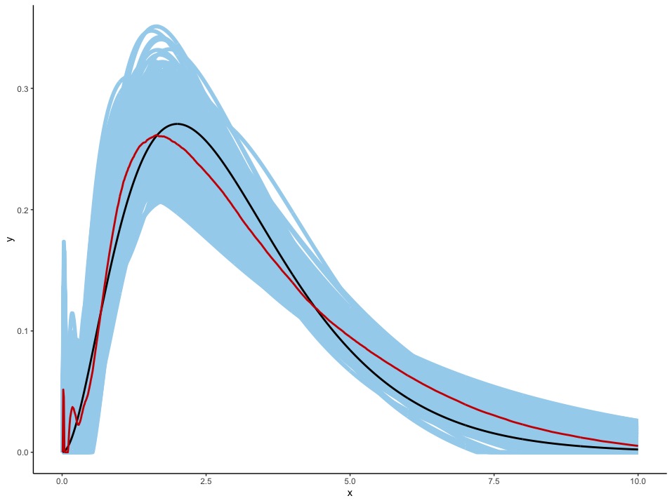
Figure 1: .Unknown error distribution, $n=1000$, $m=100$. Black line: true density $f_{1}$, Blue lines: $N$ Monte-Carlo estimations of $f_{1}$, Red Line: point-wise median. $\operatorname{eMISE}=0.00575$.

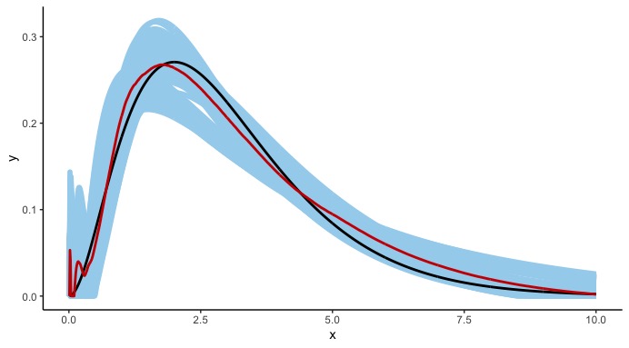
Figure 2: .Unknown error distribution, $n=1000$, $m=1000$. Black line: true density $f_{1}$, Blue lines: $N$ Monte-Carlo estimations of $f_{1}$, Red Line: point-wise median. $\operatorname{eMISE}=0.00458$.

Figure 3: .Unknown error distribution, $n=1000$, $m=4000$. Black line: true density $f_{1}$, Blue lines: $N$ Monte-Carlo estimations of $f_{1}$, Red Line: Point-wise median. $\operatorname{eMISE}=0.00449$.

Figure 4: .Known error distribution, $n=1000$. Black line: true density $f_{1}$, Blue lines: $N$ Monte-Carlo estimations of $f_{1}$, Red Line: point-wise median. $\operatorname{eMISE}=0.00299$.

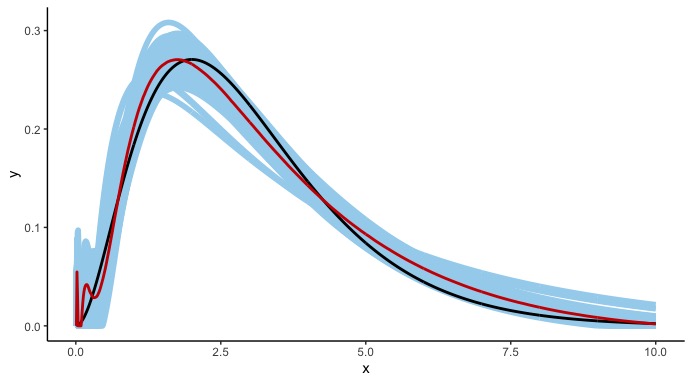
Figure 5: .Unknown error distribution, $n=m=2000$. Black line: true density $f_{1}$, Blue lines: $N$ Monte-Carlo estimations of $f_{1}$, Red Line: point-wise median. $\operatorname{eMISE}=0.00184$.

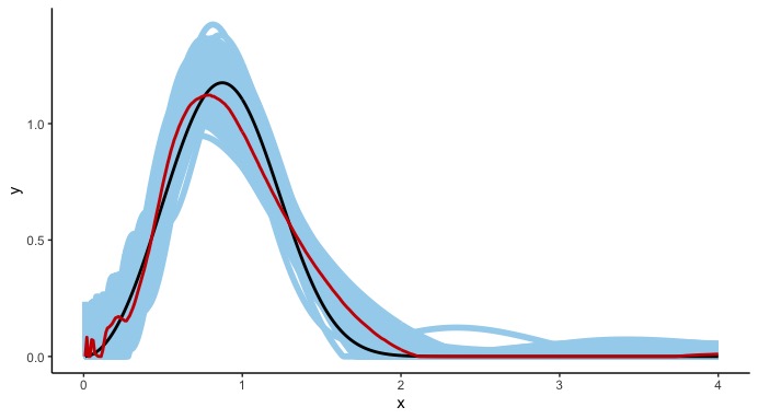
Figure 6: .Unknown error distribution, $n=m=2000$. Black line: true density $f_{2}$, Blue lines: $N$ Monte-Carlo estimations of $f_{2}$, Red Line: point-wise median. $\operatorname{eMISE}=0.0241$.

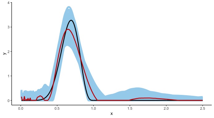
Figure 7: .Unknown error distribution, $n=m=2000$. Black line: true density $f_{3}$, Blue lines: $N$ Monte-Carlo estimations of $f_{3}$, Red Line: point-wise median. $\operatorname{eMISE}=0.129$.

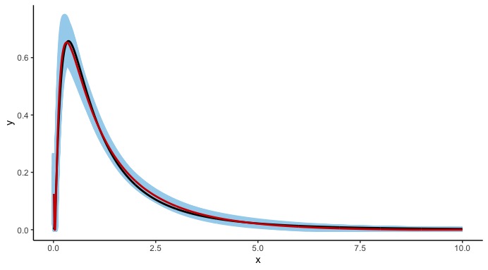
Figure 8: .Unknown error distribution, $n=m=2000$. Black line: true density $f_{4}$, Blue lines: $N$ Monte-Carlo estimations of $f_{4}$, Red Line: point-wise median. $\operatorname{eMISE}=0.00179$.

Appendix

6   6Proofs of Section 2

The next assertion provides our key argument in order to prove the concentration inequality in 2.2. The inequality is due to Talagrand [1996] and in this form for example given in Klein and Rio [2005].

Lemma § 6.1 (Talagrand’s inequality).

Let $(Z_{i})_{i\in{\left\llbracket n\right\rrbracket}}$ be independent $\mathcal{Z}$-valued random variables and let $\{\nu_{h}:h\in\mathcal{H}\}$ be countable class of Borel-measurable functions. For $h\in\mathcal{H}$ setting $\overline{\nu}_{h}=n^{-1}\sum_{i\in{\left\llbracket n\right\rrbracket}}\left\{\nu_{h}(Z_{i})-\mathbb{E}\left(\nu_{h}(Z_{i})\right)\right\}$ we have

$$\mathbb{E}\left[\left(\sup_{h\in\mathcal{H}}\{|\overline{\nu}_{h}|^{2}\}-6\Psi^{2}\right)_{+}\right]\leq\mathfrak{C}_{\mathrm{tal}}\left[\frac{\tau}{n}\exp\left(\frac{-n\Psi^{2}}{6\tau}\right)+\frac{\psi^{2}}{n^{2}}\exp\left(\frac{-n\Psi}{100\psi}\right)\right]$$ (6.1)

for some universal numerical constants $\mathfrak{C}_{\mathrm{tal}}\in\mathbb{R}_{>0}$ and where

$$\sup_{h\in\mathcal{H}}\left\{\sup_{z\in\mathcal{Z}}\left\{|\nu_{h}(z)|\right\}\right\}\leq\psi,\qquad\mathbb{E}\left[\sup_{h\in\mathcal{H}}\{|\overline{\nu}_{h}|\}\right]\leq\Psi,\qquad\sup_{h\in\mathcal{H}}\left\{n\mathbb{E}\big{[}|\overline{\nu}_{h}|^{2}\big{]}\right\}\leq\tau.$$

Remark § 6.2.

Consider an arbitrary density function $\mathrm{w}:\mathbb{R}\to\mathbb{R}_{\geq 0}$ such that $\mathds{1}_{[-k,k]}\in\mathbb{L}^{\infty}(\mathrm{w})$ for each $k\in\mathbb{R}_{>0}$. For $k\in\mathbb{R}_{>0}$ let us briefly reconsider the orthogonal projection $(\widehat{\operatorname{M}}_{Y}-\operatorname{M}_{Y})\mathds{1}_{[-k,k]}$. Introduce the subset $\mathbb{S}_{k}:=\{h\mathds{1}_{[-k,k]}:h\in\mathbb{L}^{2}(\mathrm{w})\}$ of $\mathbb{L}^{2}(\mathrm{w})$ and the unit ball $\mathbb{B}_{k}:=\{h\in\mathbb{S}_{k}:\left\|h\right\|_{\mathbb{L}^{2}(\mathrm{w})}\leq 1\}$ in $\mathbb{S}_{k}$. Clearly, setting $\kappa:\mathbb{R}_{>0}\times\mathbb{R}\to\mathbb{C}$ with $(y,t)\mapsto\kappa(y,t):=y^{c-1}y^{\iota 2\pi t}$ we have $\widehat{\operatorname{M}}_{Y}(t)=\tfrac{1}{n}\sum_{i\in{\left\llbracket n\right\rrbracket}}\kappa(Y_{i},t)$ and $\operatorname{M}_{Y}(t)=\mathbb{E}\big{[}\kappa(Y_{i},t)\big{]}$ for each $t\in\mathbb{R}$. Introducing $\kappa_{y}:\mathbb{R}\to\mathbb{C}$ with $t\mapsto\kappa_{y}(t):=\kappa(y,t)$, $y\in\mathbb{R}_{>0}$, for each $h\in\mathbb{S}_{k}$ the function $\nu_{h}:\mathbb{R}_{>0}\to\mathbb{C}$ with $y\mapsto\nu_{h}(y):=\big{\langle}\kappa_{y},h\big{\rangle}_{\mathbb{L}^{2}(\mathrm{w})}$ is Borel-measurable, where evidently $\tfrac{1}{n}\sum_{i\in{\left\llbracket n\right\rrbracket}}\nu_{h}(Y_{i})=\big{\langle}\widehat{\operatorname{M}}_{Y},h\big{\rangle}_{\mathbb{L}^{2}(\mathrm{w})}$ and hence $\overline{\nu}_{h}=\big{\langle}\widehat{\operatorname{M}}_{Y}-\operatorname{M}_{Y},h\big{\rangle}_{\mathbb{L}^{2}(\mathrm{w})}$. Consequently, we obtain

$$\left\|(\widehat{\operatorname{M}}_{Y}-\operatorname{M}_{Y})\mathds{1}_{[-k,k]}\right\|^{2}_{\mathbb{L}^{2}(\mathrm{w})}=\sup\{|\big{\langle}\widehat{\operatorname{M}}_{Y}-\operatorname{M}_{Y},h\big{\rangle}_{\mathbb{L}^{2}(\mathrm{w})}|^{2}:h\in\mathbb{B}_{k}\}=\sup\{|\overline{\nu}_{h}|^{2}:h\in\mathbb{B}_{k}\}.$$ (6.2)

Note that, the unit ball $\mathbb{B}_{k}$ is not a countable set, however, it contains a countable dense subset, say $\mathcal{B}_{k}$, since $\mathbb{L}^{2}(\mathrm{w})$ is separable. Exploiting the continuity of the inner product it is straightforward to see that

$$\left\|(\widehat{\operatorname{M}}_{Y}-\operatorname{M}_{Y})\mathds{1}_{[-k,k]}\right\|^{2}_{\mathbb{L}^{2}(\mathrm{w})}=\sup\{|\overline{\nu}_{h}|^{2}:h\in\mathbb{B}_{k}\}=\sup\{|\overline{\nu}_{h}|^{2}:h\in\mathcal{B}_{k}\}.$$

The last identity provides the necessary argument to apply below Talagrand’s inequality (6.1) where we need to calculate the three constants $\psi$, $\Psi$ and $\tau$. We note that the function $\kappa:\mathbb{R}_{>0}\times\mathbb{R}\to\mathbb{C}$ is not bounded. Therefore we decompose $\kappa=\kappa^{\mathrm{b}}+\kappa^{\mathrm{u}}$ into a bounded function $\kappa^{\mathrm{b}}:\mathbb{R}_{>0}\times\mathbb{R}\to\mathbb{C}$ with $(y,t)\mapsto\kappa^{\mathrm{b}}(y,t):=y^{c-1}\mathds{1}_{(0,d)}(y^{c-1})y^{\iota 2\pi t}$ and an unbounded function $\kappa^{\mathrm{u}}:\mathbb{R}_{>0}\times\mathbb{R}\to\mathbb{C}$ with $(y,t)\mapsto\kappa^{\mathrm{u}}(y,t):=y^{c-1}\mathds{1}_{[d,\infty)}(y^{c-1})y^{\iota 2\pi t}$ where $d:=n^{1/3}$. For $\mathrm{j}\in\{\mathrm{b},\mathrm{u}\}$ setting $\widehat{\operatorname{M}}_{Y}^{\mathrm{j}}(t)=\tfrac{1}{n}\sum_{i\in{\left\llbracket n\right\rrbracket}}\kappa^{\mathrm{j}}(Y_{i},t)$ and $\operatorname{M}_{Y}^{\mathrm{j}}(t)=\mathbb{E}\big{[}\kappa^{\mathrm{j}}(Y_{i},t)\big{]}$ for each $t\in\mathbb{R}$ it follows $\widehat{\operatorname{M}}_{Y}-\operatorname{M}_{Y}=\widehat{\operatorname{M}}_{Y}^{\mathrm{b}}-\operatorname{M}_{Y}^{\mathrm{b}}+\widehat{\operatorname{M}}_{Y}^{\mathrm{u}}-\operatorname{M}_{Y}^{\mathrm{u}}$. Introducing further $\nu_{h}^{\mathrm{b}}:\mathbb{R}_{>0}\to\mathbb{C}$ with $y\mapsto\nu_{h}^{\mathrm{b}}(y):=\big{\langle}\kappa_{y}^{\mathrm{b}},h\big{\rangle}_{\mathbb{L}^{2}(\mathrm{w})}$ and $\nu_{h}^{\mathrm{u}}:\mathbb{R}_{>0}\to\mathbb{C}$ with $y\mapsto\nu_{h}^{\mathrm{u}}(y):=\big{\langle}\kappa_{y}^{\mathrm{u}},h\big{\rangle}_{\mathbb{L}^{2}(\mathrm{w})}$ we evidently have $\overline{\nu}_{h}=\overline{\nu}_{h}^{\mathrm{b}}+\overline{\nu}_{h}^{\mathrm{u}}$ and thus

$$\left\|(\widehat{\operatorname{M}}_{Y}-\operatorname{M}_{Y})\mathds{1}_{[-k,k]}\right\|^{2}_{\mathbb{L}^{2}(\mathrm{w})} =\sup\{|\overline{\nu}_{h}|^{2}:h\in\mathcal{B}_{k}\}=\sup\{|\overline{\nu}_{h}^{\mathrm{b}}+\overline{\nu}_{h}^{\mathrm{u}}|^{2}:h\in\mathcal{B}_{k}\}$$

$$\hskip 21.52771pt\leq 2\sup\{|\overline{\nu}_{h}^{\mathrm{b}}|^{2}:h\in\mathcal{B}_{k}\}+2\sup\{|\overline{\nu}_{h}^{\mathrm{u}}|^{2}:h\in\mathcal{B}_{k}\}\hfill$$

$$\hskip 21.52771pt=2\left\|(\widehat{\operatorname{M}}_{Y}^{\mathrm{b}}-\operatorname{M}_{Y}^{\mathrm{b}})\mathds{1}_{[-k,k]}\right\|^{2}_{\mathbb{L}^{2}(\mathrm{w})}+2\left\|(\widehat{\operatorname{M}}_{Y}^{\mathrm{u}}-\operatorname{M}_{Y}^{\mathrm{u}})\mathds{1}_{[-k,k]}\right\|^{2}_{\mathbb{L}^{2}(\mathrm{w})}.$$ (6.3)

In 6.3 below we bound the expectation of the first term on the right hand side with the help of Talagrand’s inequality (6.1) and the expectation of the second term.∎

Lemma § 6.3.

Let $\mathrm{w}:\mathbb{R}\to\mathbb{R}_{\geq 0}$ be a density function, such that $\mathds{1}_{[-k,k]}\in\mathbb{L}^{\infty}(\mathrm{w})$ for each $k\in\mathbb{R}_{>0}$. Setting $\sigma_{Y}^{2}:=1+\mathbb{E}[Y_{1}^{2(c-1)}]$, $a_{Y}:=6\left\|f^{Y}\right\|_{\mathbb{L}^{\infty}(\mathrm{x}^{2c-1})}/\sigma_{Y}^{2}$, $k_{Y}:=1\vee 3a_{Y}^{2}$,

$$\Delta_{k}^{\mathrm{w}}:=\left\|\mathds{1}_{[-k,k]}\right\|_{\mathbb{L}^{\infty}(\mathrm{w})}\text{ and }\delta_{k}^{\mathrm{w}}:=\frac{\log(\Delta_{k}^{\mathrm{w}}\lor(k+2))}{\log(k+2)}\in\mathbb{R}_{\geq 1},\quad\forall k\in\mathbb{R}_{\geq 1},$$

there exists an universal numerical constant $\mathfrak{C}\in\mathbb{R}_{>0}$ such that for all $n\in\mathbb{N}$ and $k\in\mathbb{R}_{\geq 1}$ we have

$$\mathbb{E}\left[\left(\left\|\mathds{1}_{[-k,k]}(\widehat{\operatorname{M}}_{Y}^{\mathrm{b}}-\operatorname{M}_{Y}^{\mathrm{b}})\right\|^{2}_{\mathbb{L}^{2}(\mathrm{w})}-6\sigma_{Y}^{2}\Delta_{k}^{\mathrm{w}}\delta_{k}^{\mathrm{w}}kn^{-1}\right)_{+}\right]\\ \leq n^{-1}\times\mathfrak{C}\times\bigg{[}(1\vee\left\|f^{Y}\right\|_{\mathbb{L}^{\infty}(\mathrm{x}^{2c-1})}^{2})(1+\left\|\mathds{1}_{[-k_{Y},k_{Y}]}\right\|_{\mathbb{L}^{2}(\mathrm{w})}^{2})\frac{1}{a_{Y}}\exp\big{(}\frac{-k}{a_{Y}}\big{)}+n^{-4}k\Delta_{k}^{\mathrm{w}}\bigg{]}$$ (6.4)

and $\mathbb{E}\left[\left\|\mathds{1}_{[-k,k]}(\widehat{\operatorname{M}}_{Y}^{\mathrm{u}}-\operatorname{M}_{Y}^{\mathrm{u}})\right\|^{2}_{\mathbb{L}^{2}(\mathrm{w})}\right]\leq 2\mathbb{E}\big{[}Y_{1}^{8(c-1)}\big{]}n^{-3}k\Delta_{k}^{\mathrm{w}}$.

Proof of 5 (6.3).

Consider first the second claim. For each $t\in\mathbb{R}$ we have $\mathbb{E}\big{[}\widehat{\operatorname{M}}_{Y}^{\mathrm{u}}(t)\big{]}=\operatorname{M}_{Y}^{\mathrm{u}}(t)=\mathbb{E}\big{[}\kappa^{\mathrm{u}}(Y_{1},t)\big{]}$ which in turn implies

$$n\mathbb{E}\big{[}|\widehat{\operatorname{M}}_{Y}^{\mathrm{u}}(t)-\operatorname{M}_{Y}^{\mathrm{u}}(t)|^{2}\big{]} =\mathbb{V}\mathrm{ar}\big{(}\kappa^{\mathrm{u}}(Y_{1},t)\big{)}\leq\mathbb{E}\big{[}|\kappa^{\mathrm{u}}(Y_{1},t)|^{2}\big{]}=\mathbb{E}\big{[}Y_{1}^{2(c-1)}\mathds{1}_{[d,\infty)}(Y_{1}^{c-1})]\leq d^{-2l}\mathbb{E}\big{[}Y_{1}^{2(c-1)(1+l)}\big{]}$$

and thus making use of $d=n^{1/3}$ we obtain the claim, that is

$$\mathbb{E}\left[\left\|\mathds{1}_{[-k,k]}(\widehat{\operatorname{M}}_{Y}^{\mathrm{u}}-\operatorname{M}_{Y}^{\mathrm{u}})\right\|^{2}_{\mathbb{L}^{2}(\mathrm{w})}\right] \leq\tfrac{1}{nd^{6}}\mathbb{E}\big{[}Y_{1}^{2(c-1)(1+3)}\big{]}\left\|\mathds{1}_{[-k,k]}\right\|^{2}_{\mathbb{L}^{2}(\mathrm{w})}\leq n^{-3}\mathbb{E}\big{[}Y_{1}^{8(c-1)}\big{]}2k\Delta_{k}^{\mathrm{w}}.$$

Secondly consider (6.4). Given the identity (see Remark 6.2)

$$\left\|(\widehat{\operatorname{M}}_{Y}^{\mathrm{b}}-\operatorname{M}_{Y}^{\mathrm{b}})\mathds{1}_{[-k,k]}\right\|^{2}_{\mathbb{L}^{2}(\mathrm{w})}=\sup\{|\overline{\nu}_{h}^{\mathrm{b}}|^{2}:h\in\mathcal{B}_{k}\}$$

we intent to apply Talagrand’s inequality (6.1) where we need to calculate the three quantities $\psi$, $\Psi$ and $\tau$. Consider $\psi$ first. Evidently, for each $k\in\mathbb{R}_{\geq 1}$ we have

$$\sup_{h\in\mathcal{B}_{k}}\left\{\sup_{y\in\mathbb{R}_{>0}}\left\{|\nu_{h}^{\mathrm{b}}(y)|^{2}\right\}\right\}=\sup_{y\in\mathbb{R}_{>0}}\left\{\sup_{h\in\mathcal{B}_{k}}\left\{|\big{\langle}\kappa_{y}^{\mathrm{b}},h\big{\rangle}_{\mathbb{L}^{2}(\mathrm{w})}|^{2}\right\}\right\}\\ =\sup_{y\in\mathbb{R}_{>0}}\left\{\left\|\kappa_{y}^{\mathrm{b}}\mathds{1}_{[-k,k]}\right\|_{\mathbb{L}^{2}(\mathrm{w})}^{2}\right\}\leq d^{2}\left\|\mathds{1}_{[-k,k]}\right\|_{\mathbb{L}^{2}(\mathrm{w})}^{2}\leq 2d^{2}k\Delta_{k}^{\mathrm{w}}=:\psi^{2}.$$

Consider next $\Psi$. Evidently, for each $t\in\mathbb{R}$ we have

$$n\mathbb{E}\big{[}|\widehat{\operatorname{M}}_{Y}^{\mathrm{b}}(t)-\operatorname{M}_{Y}^{\mathrm{b}}(t)|^{2}\big{]}=\mathbb{V}\mathrm{ar}\big{(}\kappa^{\mathrm{b}}(Y_{1},t)\big{)}\leq\mathbb{E}\big{[}|\kappa^{\mathrm{b}}(Y_{1},t)|^{2}\big{]}\leq\mathbb{E}\big{[}Y_{1}^{2(c-1)}\big{]}\leq\sigma_{Y}^{2}$$

which for each $k\in\mathbb{R}_{\geq 1}$ implies

$$\mathbb{E}\left[\sup_{h\in\mathcal{H}}|\overline{\nu}_{h}^{\mathrm{b}}|^{2}\right] =\mathbb{E}\left[\left\|(\widehat{\operatorname{M}}_{Y}^{\mathrm{b}}-\operatorname{M}_{Y}^{\mathrm{b}})\mathds{1}_{[-k,k]}\right\|^{2}_{\mathbb{L}^{2}(\mathrm{w})}\right]\leq\tfrac{1}{n}\sigma_{Y}^{2}\left\|\mathds{1}_{[-k,k]}\right\|_{\mathbb{L}^{2}(\mathrm{w})}^{2}\leq\tfrac{1}{n}\sigma_{Y}^{2}2k\Delta_{k}^{\mathrm{w}}\delta_{k}^{\mathrm{w}}=:\Psi^{2}.$$

Finally, consider $\tau$. For each $h\in\mathcal{B}_{k}$ we have

$$n\mathbb{E}\big{[}|\overline{\nu}_{h}^{\mathrm{b}}|^{2}\big{]}=\mathbb{V}\mathrm{ar}\big{[}\big{\langle}\kappa^{\mathrm{b}}(Y_{1},\cdot),h\big{\rangle}_{\mathbb{L}^{2}(\mathrm{w})}\big{]} \leq\mathbb{E}\big{[}|\big{\langle}\kappa^{\mathrm{b}}(Y_{1},\cdot),h\big{\rangle}_{\mathbb{L}^{2}(\mathrm{w})}|^{2}\big{]}\leq\mathbb{E}\big{[}|\big{\langle}\kappa(Y_{1},\cdot),h\big{\rangle}_{\mathbb{L}^{2}(\mathrm{w})}|^{2}\big{]}=\mathbb{E}\big{[}|\nu_{h}|^{2}\big{]}.$$

Since $h\mathrm{w}\in\mathbb{L}^{2}\cap\mathbb{L}^{1}$ and $|\nu_{h}(y)|^{2}=|\big{\langle}h,\kappa_{y}\big{\rangle}_{\mathbb{L}^{2}(\mathrm{w})}|^{2}=|\operatorname{M}_{1-c}^{-1}[h\mathrm{w}](y)|^{2}$ for all $y\in\mathbb{R}_{>0}$ we have $\nu_{h}\in\mathbb{L}^{2}(\mathrm{x}^{1-2c})$. Consequently, using Parseval’s identity we obtain

$$\left\|\nu_{h}\right\|_{\mathbb{L}^{2}(\mathrm{x}^{1-2c})}^{2}=\left\|\operatorname{M}_{1-c}[\nu_{h}]\right\|_{\mathbb{L}^{2}}^{2}=\left\|\mathrm{w}h\right\|_{\mathbb{L}^{2}}^{2}\leq\left\|\mathrm{w}\mathds{1}_{[-k,k]}\right\|_{\mathbb{L}^{\infty}}\left\|h\right\|_{\mathbb{L}^{2}(\mathrm{w})}^{2}\leq\Delta_{k}^{\mathrm{w}}$$

which in turn for each $h\in\mathcal{B}_{k}$ implies

$$\mathbb{E}\big{[}|\nu_{h}|^{2}\big{]}\leq\left\|f^{Y}\right\|_{\mathbb{L}^{\infty}(\mathrm{x}^{2c-1})}\left\|\nu_{h}\right\|_{\mathbb{L}^{2}(\mathrm{x}^{1-2c})}^{2}\leq\left\|f^{Y}\right\|_{\mathbb{L}^{\infty}(\mathrm{x}^{2c-1})}\Delta_{k}^{\mathrm{w}}.$$

On the other hand side for each $h\in\mathcal{B}_{k}$ we have also

$$\mathbb{E}\big{[}|\nu_{h}|^{2}\big{]}\leq\left\|\mathds{1}_{[-k,k]}\right\|_{\mathbb{L}^{2}(\mathrm{w})}^{2}\mathbb{E}[Y_{1}^{2(c-1)}]\leq\left\|\mathds{1}_{[-k,k]}\right\|_{\mathbb{L}^{2}(\mathrm{w})}^{2}\sigma_{Y}^{2},$$

and hence

$$n\mathbb{E}\big{[}|\overline{\nu}_{h}^{\mathrm{b}}|^{2}\big{]}\leq\left\|f^{Y}\right\|_{\mathbb{L}^{\infty}(\mathrm{x}^{2c-1})}\Delta_{k}^{\mathrm{w}}\wedge\sigma_{Y}^{2}\left\|\mathds{1}_{[-k,k]}\right\|_{\mathbb{L}^{2}(\mathrm{w})}^{2}=:\tau.$$

Given $a_{Y}=6\left\|f^{Y}\right\|_{\mathbb{L}^{\infty}(\mathrm{x}^{2c-1})}/\sigma_{Y}^{2}$ and $k_{Y}=1\vee 3a_{Y}^{2}$ for any $k\geq k_{Y}$ we have

$$\Delta_{k}^{\mathrm{w}}\exp\left(\frac{-\sigma_{Y}^{2}\delta_{k}^{\mathrm{w}}k}{6\left\|f^{Y}\right\|_{\mathbb{L}^{\infty}(\mathrm{x}^{2c-1})}}\right)=\Delta_{k}^{\mathrm{w}}\exp\big{(}\tfrac{-\delta_{k}^{\mathrm{w}}}{a_{Y}}k\big{)}\leq\exp(-\tfrac{\delta_{k}^{\mathrm{w}}}{a_{Y}}(k-a_{Y}\log(k+2))\leq 1$$

by exploiting that $x\geq a\log(x+2)$ for all $a>0$ and $x\geq 1\vee 3a^{2}$. Consequently, for any $k\geq k_{Y}$ we obtain (keep $\delta_{k}^{\mathrm{w}}\geq 1$ in mind)

$$\frac{\tau}{n}\exp\left(\frac{-n\Psi^{2}}{6\tau}\right) \leq\tfrac{\left\|f^{Y}\right\|_{\mathbb{L}^{\infty}(\mathrm{x}^{2c-1})}\Delta_{k}^{\mathrm{w}}}{n}\exp\left(\frac{-\sigma_{Y}^{2}\delta_{k}^{\mathrm{w}}k}{3\left\|f^{Y}\right\|_{\mathbb{L}^{\infty}(\mathrm{x}^{2c-1})}}\right)\leq\tfrac{\left\|f^{Y}\right\|_{\mathbb{L}^{\infty}(\mathrm{x}^{2c-1})}}{n}\exp\big{(}\frac{-k}{a_{Y}}\big{)}$$

while for any $k<k_{Y}$ we conclude (using again $\delta_{k}^{\mathrm{w}}\geq 1$)

$$\frac{\tau}{n}\exp\left(\frac{-n\Psi^{2}}{6\tau}\right) \leq\tfrac{\sigma_{Y}^{2}\left\|\mathds{1}_{[-k,k]}\right\|_{\mathbb{L}^{2}(\mathrm{w})}^{2}}{n}\exp\left(\frac{-\sigma_{Y}^{2}\delta_{k}^{\mathrm{w}}k}{3\left\|f^{Y}\right\|_{\mathbb{L}^{\infty}(\mathrm{x}^{2c-1})}}\right)\leq\tfrac{\sigma_{Y}^{2}\left\|\mathds{1}_{[-k_{Y},k_{Y}]}\right\|_{\mathbb{L}^{2}(\mathrm{w})}^{2}}{n}\exp\big{(}\frac{-k}{a_{Y}}\big{)}.$$

Combining both cases $k\geq k_{Y}$ and $k<k_{Y}$ we obtain for any $k\in\mathbb{R}_{\geq 1}$

$$\frac{\tau}{n}\exp\left(\frac{-n\Psi^{2}}{6\tau}\right)\leq\tfrac{\left\|f^{Y}\right\|_{\mathbb{L}^{\infty}(\mathrm{x}^{2c-1})}+\sigma_{Y}^{2}\left\|\mathds{1}_{[-k_{Y},k_{Y}]}\right\|_{\mathbb{L}^{2}(\mathrm{w})}^{2}}{n}\exp\big{(}\frac{-k}{a_{Y}}\big{)}.$$

Evaluating the bound given by Talagrand’s inequality (6.1) there exists an universal numerical constant $\mathfrak{C}_{\mathrm{tal}}\in\mathbb{R}_{>0}$ such that for each $k\in\mathbb{R}_{\geq 1}$ we have (keep $d=n^{1/3}$, $\sigma_{Y}^{2}\geq 1$ and $\delta_{k}^{\mathrm{w}}\geq 1$ in mind)

$$\mathbb{E}\left[\left(\left\|\mathds{1}_{[-k,k]}(\widehat{\operatorname{M}}_{Y}^{\mathrm{b}}-\operatorname{M}_{Y}^{\mathrm{b}})\right\|^{2}_{\mathbb{L}^{2}(\mathrm{w})}-6\sigma_{Y}^{2}\Delta_{k}^{\mathrm{w}}\delta_{k}^{\mathrm{w}}kn^{-1}\right)_{+}\right]$$

$$\leq n^{-1}\mathfrak{C}_{\mathrm{tal}}\bigg{[}n^{-1/3}k\Delta_{k}^{\mathrm{w}}\exp\left(\frac{-n^{1/6}}{100}\right)$$

$$\phantom{=}+(\left\|f^{Y}\right\|_{\mathbb{L}^{\infty}(\mathrm{x}^{2c-1})}+\sigma_{Y}^{2}\left\|\mathds{1}_{[-k_{Y},k_{Y}]}\right\|_{\mathbb{L}^{2}(\mathrm{w})}^{2})\exp\big{(}\frac{-k}{a_{Y}}\big{)}\bigg{]}$$

$$\leq n^{-1}\mathfrak{C}\bigg{[}n^{-4}k\Delta_{k}^{\mathrm{w}}n^{11/3}\exp\left(\frac{-n^{1/6}}{100}\right)$$

$$\phantom{=}+(1\vee\left\|f^{Y}\right\|_{\mathbb{L}^{\infty}(\mathrm{x}^{2c-1})}^{2})(1+\left\|\mathds{1}_{[-k_{Y},k_{Y}]}\right\|_{\mathbb{L}^{2}(\mathrm{w})}^{2})\frac{1}{a_{Y}}\exp\big{(}\frac{-k}{a_{Y}}\big{)}\bigg{]},$$

which together with $n^{b}\exp(-an^{1/c})\leq(\tfrac{cb}{ae})^{cb}$ for all $a,b,c\in\mathbb{R}_{>0}$, and hence $n^{11/3}\exp(\frac{-n^{1/6}}{100})\leq(1100)^{22}$ shows (6.4) and completes the proof.

7   7Proofs of Section Section 3

Lemma § 7.1.

There exists an universal numerical constant $\mathfrak{C}\in\mathbb{R}_{\geq 1}$ such that for any $k\in\mathbb{R}_{>0}$ we have

$$\mathbb{E}\left[\left\|\mathds{1}_{[-k,k]}\widehat{\operatorname{M}}_{U}^{\dagger}\mathds{1}_{\mathfrak{M}}\right\|_{\mathbb{L}^{2}(\mathrm{v})}^{2}\right]\leq 4\big{(}1\lor\mathbb{E}[U_{1}^{2(c-1)}]\big{)}\left\|\mathds{1}_{[-k,k]}\operatorname{M}_{U}^{\dagger}\right\|_{\mathbb{L}^{2}(\mathrm{v})}^{2},$$

$$\mathbb{E}\left[\left\|\mathds{1}_{[-k,k]}\operatorname{M}_{X}\mathds{1}_{\mathfrak{M}^{C}}\right\|_{\mathbb{L}^{2}(\mathrm{v})}^{2}\right]\leq 4\big{(}1\lor\mathbb{E}[U_{1}^{2(c-1)}]\big{)}\left\|\mathds{1}_{[-k,k]}\operatorname{M}_{X}\big{(}1\vee|\operatorname{M}_{U}|^{2}(m\land n)\big{)}^{-1/2}\right\|_{\mathbb{L}^{2}(\mathrm{v})}^{2},$$

$$\mathbb{E}\left[\left\|\mathds{1}_{[-k,k]}\operatorname{M}_{X}(\operatorname{M}_{U}-\widehat{\operatorname{M}}_{U})\widehat{\operatorname{M}}_{U}^{\dagger}\mathds{1}_{\mathfrak{M}}\right\|_{\mathbb{L}^{2}(\mathrm{v})}^{2}\right]\leq 4\big{(}1\lor\mathfrak{C}\,\mathbb{E}[U_{1}^{4(c-1)}]\big{)}\left\|\mathds{1}_{[-k,k]}\operatorname{M}_{X}\big{(}1\vee|\operatorname{M}_{U}|^{2}m\big{)}^{-1/2}\right\|_{\mathbb{L}^{2}(\mathrm{v})}^{2}.$$

Proof of 6 (7.1).

We start our proof with the observation that for each $t\in\mathbb{R}$ we have $\mathbb{E}[\widehat{\operatorname{M}}_{U}(t)]=\operatorname{M}_{U}(t)$, $m\mathbb{E}\big{[}|\widehat{\operatorname{M}}_{U}(t)-\operatorname{M}_{U}(t)|^{2}\big{]}\leq\mathbb{E}[U_{1}^{2(c-1)}]$, and $m^{2}\mathbb{E}\big{[}|\widehat{\operatorname{M}}_{U}(t)-\operatorname{M}_{U}(t)|^{4}\big{]}\leq\mathfrak{C}\,\mathbb{E}[U_{1}^{4(c-1)}]$ for some universal numerical constant $\mathfrak{C}\in\mathbb{R}_{\geq 1}$ by applying Theorem 2.10 in Petrov [1995]. We use those bounds without further reference. Below we show that for each $t\in\mathbb{R}$ we have

$$\mathbb{E}\left[|\operatorname{M}_{U}(t)\widehat{\operatorname{M}}_{U}^{\dagger}(t)|^{2}\mathds{1}_{\mathfrak{M}}(t)\right]\leq 4\big{(}1\lor\mathbb{E}[U_{1}^{2(c-1)}]\big{)}$$ (7.1)

$$\mathbb{E}\left[\mathds{1}_{\mathfrak{M}^{C}}(t)\right]=\mathbb{P}\left((n\land m)|\widehat{\operatorname{M}}_{U}(t)|^{2}<1\right)\leq 4\big{(}1\lor\mathbb{E}[U_{1}^{2(c-1)}]\big{)}\big{(}1\vee|\operatorname{M}_{U}(t)|^{2}(m\land n)\big{)}^{-1}$$

$$\mathbb{E}\left[|\operatorname{M}_{U}(t)-\widehat{\operatorname{M}}_{U}(t)|^{2}|\widehat{\operatorname{M}}_{U}^{\dagger}(t)|^{2}\mathds{1}_{\mathfrak{M}}(t)\right]\leq 4\big{(}1\lor\mathfrak{C}\,\mathbb{E}[U_{1}^{4(c-1)}])\big{)}(1\vee|\operatorname{M}_{U}(t)|^{2}m)^{-1}$$ (7.2)

Evidently, by applying Fubini’s theorem from the last bounds follow immediatly 7.1. It remains to show ((7.1)-(7.2)). Let $t\in\mathbb{R}$ be fixed. Consider (7.1) first. Exploiting $|\widehat{\operatorname{M}}_{U}(t)\widehat{\operatorname{M}}_{U}^{\dagger}(t)|^{2}\mathds{1}_{\mathfrak{M}}(t)=\mathds{1}_{\mathfrak{M}}(t)$ and $2|\widehat{\operatorname{M}}_{U}(t)|^{2}+2|\operatorname{M}_{U}(t)-\widehat{\operatorname{M}}_{U}(t)|^{2}\geq|\operatorname{M}_{U}(t)|^{2}$ we have

$$\mathbb{E}\left[|\operatorname{M}_{U}(t)\widehat{\operatorname{M}}_{U}^{\dagger}(t)|^{2}\mathds{1}_{\mathfrak{M}}(t)\right] \leq 2\mathbb{E}\left[|\operatorname{M}_{U}(t)-\widehat{\operatorname{M}}_{U}(t)|^{2}|\widehat{\operatorname{M}}_{U}^{\dagger}(t)|^{2}\mathds{1}_{\mathfrak{M}}(t)+\mathds{1}_{\mathfrak{M}}(t)\right]$$

$$\leq 2\left((m\land n)\mathbb{E}[|\operatorname{M}_{U}(t)-\widehat{\operatorname{M}}_{U}(t)|^{2}]+1\right)$$

$$\leq 2\left(\mathbb{E}[U_{1}^{2(c-1)}]+1\right)\leq 4\left(1\lor\mathbb{E}[U_{1}^{2(c-1)}]\right)$$

which shows (7.1). Secondly, (7.2) is trivially satisfied if $1\leq 4(1\lor\mathbb{E}[U_{1}^{2(c-1)}])(1\lor|\operatorname{M}_{U}(t)|^{2}(n\land m))^{-1}$. Otherwise, from $(1\lor|\operatorname{M}_{U}(t)|^{2}(n\land m))>4(1\lor\mathbb{E}[U_{1}^{2(c-1)}])\geq 4$ follows $(n\land m)^{-1}<|\operatorname{M}_{U}(t)|^{2}/4$ which using Markov’s inequality implies (LABEL:lem:2:p2), that is

$$\mathbb{P}\left(|\widehat{\operatorname{M}}_{U}(t)|^{2}<(n\land m)^{-1}\right) \leq\mathbb{P}\left(|\widehat{\operatorname{M}}_{U}(t)-\operatorname{M}_{U}(t)|>|\operatorname{M}_{U}(t)|/2\right)$$

$$\leq 4\mathbb{E}\big{[}|\widehat{\operatorname{M}}_{U}(t)-\operatorname{M}_{U}(t)|^{2}\big{]}|\operatorname{M}_{U}(t)|^{-2}$$

$$\leq 4\mathbb{E}[U_{1}^{2(c-1)}](|\operatorname{M}_{U}(t)|^{2}m)^{-1}$$

$$\leq 4(1\lor\mathbb{E}[U_{1}^{2(c-1)}])(1\lor|\operatorname{M}_{U}(t)|^{2}(n\land m))^{-1}.$$

Finally, consider (7.2). Evidently, we have on the one hand

$$\mathbb{E}\left[|\operatorname{M}_{U}(t)-\widehat{\operatorname{M}}_{U}(t)|^{2}|\widehat{\operatorname{M}}_{U}^{\dagger}(t)|^{2}\mathds{1}_{\mathfrak{M}}(t)\right]\leq(n\land m)m^{-1}\mathbb{E}[U_{1}^{2(c-1)}]\leq\mathbb{E}[U_{1}^{2(c-1)}]$$

while on the other hand

$$\mathbb{E}\left[|\operatorname{M}_{U}(t)-\widehat{\operatorname{M}}_{U}(t)|^{2}|\widehat{\operatorname{M}}_{U}^{\dagger}(t)|^{2}\mathds{1}_{\mathfrak{M}}(t)\right]\\ \leq 2\mathbb{E}\left[|\operatorname{M}_{U}(t)-\widehat{\operatorname{M}}_{U}(t)|^{2}|\widehat{\operatorname{M}}_{U}^{\dagger}(t)|^{2}\mathds{1}_{\mathfrak{M}}(t)\big{(}\frac{|\operatorname{M}_{U}(t)-\widehat{\operatorname{M}}_{U}(t)|^{2}}{|\operatorname{M}_{U}(t)|^{2}}+\frac{|\widehat{\operatorname{M}}_{U}(t)|^{2}}{|\operatorname{M}_{U}(t)|^{2}}\big{)}\right]\\ \leq 2\frac{(m\land n)\mathbb{E}\big{[}|\operatorname{M}_{U}(t)-\widehat{\operatorname{M}}_{U}(t)|^{4}\big{]}}{|\operatorname{M}_{U}(t)|^{2}}+2\frac{\mathbb{E}\big{[}|\operatorname{M}_{U}(t)-\widehat{\operatorname{M}}_{U}(t)|^{2}\big{]}}{|\operatorname{M}_{U}(t)|^{2}}\\ \leq 2(\mathfrak{C}\mathbb{E}[U_{1}^{4(c-1)}]+\mathbb{E}[U_{1}^{2(c-1)}])(|\operatorname{M}_{U}(t)|^{2}m)^{-1}.$$

Combining both bounds we obtain (7.2), which completes the proof.

8   8Proofs of Section Section 4

We first recall an inequality due to Talagrand [1996] which in this form for example is stated by Birgé and Massart [1998] in equation (5.13) in Corollary 2. We make use of it in the proof of 4.5 below.

Lemma § 8.1 (Talagrand’s inequality).

Let $(Z_{i})_{i\in{\left\llbracket m\right\rrbracket}}$ be independent and identically distributed $\mathcal{Z}$-valued random variables and let $\{\nu_{t}:t\in\mathcal{T}\}$ be countable class of Borel-measurable functions. For $t\in\mathcal{T}$ setting

$$\overline{\nu}_{t}=m^{-1}\sum_{i\in{\left\llbracket m\right\rrbracket}}\left\{\nu_{t}(Z_{i})-\mathbb{E}\left(\nu_{t}(Z_{i})\right)\right\}$$

we have

$$\mathbb{P}\left[\sup_{t\in\mathcal{T}}|\overline{\nu}_{t}|\geq 2\Psi+\kappa\right]\leq 3\exp\left(-\mathfrak{C}_{\mathrm{tal}}m\big{(}\frac{\kappa^{2}}{\tau}\wedge\frac{\kappa}{\psi}\big{)}\right)$$ (8.1)

for some universal numerical constant $\mathfrak{C}_{\mathrm{tal}}\in\mathbb{R}_{>0}$ and where

$$\sup_{t\in\mathcal{T}}\left\{\sup_{z\in\mathcal{Z}}\left\{|\nu_{t}(z)|\right\}\right\}\leq\psi,\qquad\mathbb{E}\left[\sup_{t\in\mathcal{T}}|\overline{\nu}_{t}|\right]\leq\Psi,\qquad\sup_{t\in\mathcal{T}}\left\{\mathbb{E}\big{[}|\nu_{t}(Z_{1})|^{2}\big{]}\right\}\leq\tau.$$

Proof of 7 (4.1).

Let $k_{\circ}\in\mathcal{K}:={\left\llbracket k_{n}\right\rrbracket}$ be arbitrary but fixed. Introduce $\widehat{\operatorname{M}}_{X}:=\widehat{\operatorname{M}}_{Y}\widehat{\operatorname{M}}_{U}^{\dagger}\mathds{1}_{\mathfrak{M}}$ and $\widecheck{\operatorname{M}}_{X}:=\operatorname{M}_{Y}\widehat{\operatorname{M}}_{U}^{\dagger}\mathds{1}_{\mathfrak{M}}=\operatorname{M}_{X}\operatorname{M}_{U}\widehat{\operatorname{M}}_{U}^{\dagger}\mathds{1}_{\mathfrak{M}}$, for each $k\in\mathbb{R}_{>0}$ we write shortly $\widehat{\operatorname{M}}_{X}^{k}:=\widehat{\operatorname{M}}_{X}\mathds{1}_{[-k,k]}$, $\widecheck{\operatorname{M}}_{X}^{k}:=\widecheck{\operatorname{M}}_{X}\mathds{1}_{[-k,k]}$ and $\operatorname{M}_{X}^{k}:=\operatorname{M}_{X}\mathds{1}_{[-k,k]}$. Consider the disjoint decomposition $\mathcal{K}=\mathcal{K}_{<k_{\circ}}\cup\mathcal{K}_{\geq k_{\circ}}$ where $\mathcal{K}_{<k_{\circ}}:=\{k\in\mathcal{K}:k<k_{\circ}\}$ and $\mathcal{K}_{\geq k_{\circ}}:=\{k\in\mathcal{K}:k\geq k_{\circ}\}$, and similarly $\mathcal{K}=\mathcal{K}_{\leq k_{\circ}}\cup\mathcal{K}_{>k_{\circ}}$. Evidently, we have

$$\mathds{1}_{[-\hat{k},\hat{k}]}\widehat{\operatorname{M}}_{Y}\widehat{\operatorname{M}}_{U}^{\dagger}\mathds{1}_{\mathfrak{M}}-\operatorname{M}_{X}=\widehat{\operatorname{M}}_{X}^{\hat{k}}-\widecheck{\operatorname{M}}_{X}^{\hat{k}}+(\widecheck{\operatorname{M}}_{X}^{\hat{k}}-\widecheck{\operatorname{M}}_{X}^{k_{\circ}})\mathds{1}_{\hat{k}\in\mathcal{K}_{<k_{\circ}}}+(\widecheck{\operatorname{M}}_{X}^{k_{\circ}}-\operatorname{M}_{X})\mathds{1}_{\hat{k}\in\mathcal{K}_{<k_{\circ}}}+(\widecheck{\operatorname{M}}_{X}^{\hat{k}}-\operatorname{M}_{X})\mathds{1}_{\hat{k}\in\mathcal{K}_{\geq k_{\circ}}}$$

which in turn implies

$$\left\|\widehat{\operatorname{M}}_{X}^{\hat{k}}-\operatorname{M}_{X}\right\|_{\mathbb{L}^{2}(\mathrm{v})}^{2}\leq 3\left\|\widehat{\operatorname{M}}_{X}^{\hat{k}}-\widecheck{\operatorname{M}}_{X}^{\hat{k}}\right\|_{\mathbb{L}^{2}(\mathrm{v})}^{2}+3\left\|\widecheck{\operatorname{M}}_{X}^{\hat{k}}-\widecheck{\operatorname{M}}_{X}^{k_{\circ}}\right\|_{\mathbb{L}^{2}(\mathrm{v})}^{2}\mathds{1}_{\hat{k}\in\mathcal{K}_{<k_{\circ}}}\\ +3\big{(}\left\|\widecheck{\operatorname{M}}_{X}^{k_{\circ}}-\operatorname{M}_{X}\right\|_{\mathbb{L}^{2}(\mathrm{v})}^{2}\mathds{1}_{\hat{k}\in\mathcal{K}_{<k_{\circ}}}+\left\|\widecheck{\operatorname{M}}_{X}^{\hat{k}}-\operatorname{M}_{X}\right\|_{\mathbb{L}^{2}(\mathrm{v})}^{2}\mathds{1}_{\hat{k}\in\mathcal{K}_{\geq k_{\circ}}}\big{)}.$$

Combining the last bound and the elementary estimate (keep in mind that $k_{n}:=\max\mathcal{K}$)

$$\left\|\widecheck{\operatorname{M}}_{X}^{k_{\circ}}-\operatorname{M}_{X}\right\|_{\mathbb{L}^{2}(\mathrm{v})}^{2}\mathds{1}_{\hat{k}\in\mathcal{K}_{<k_{\circ}}}+\left\|\widecheck{\operatorname{M}}_{X}^{\hat{k}}-\operatorname{M}_{X}\right\|_{\mathbb{L}^{2}(\mathrm{v})}^{2}\mathds{1}_{\hat{k}\in\mathcal{K}_{\geq k_{\circ}}}\leq\left\|\widecheck{\operatorname{M}}_{X}^{k_{n}}-\operatorname{M}_{X}^{k_{n}}\right\|_{\mathbb{L}^{2}(\mathrm{v})}^{2}+\left\|\operatorname{M}_{X}^{k_{\circ}}-\operatorname{M}_{X}\right\|_{\mathbb{L}^{2}(\mathrm{v})}^{2}$$

we have

$$\left\|\widehat{\operatorname{M}}_{X}^{\hat{k}}-\operatorname{M}_{X}\right\|_{\mathbb{L}^{2}(\mathrm{v})}^{2}\leq 3\left\|\widehat{\operatorname{M}}_{X}^{\hat{k}}-\widecheck{\operatorname{M}}_{X}^{\hat{k}}\right\|_{\mathbb{L}^{2}(\mathrm{v})}^{2}+3\left\|\widecheck{\operatorname{M}}_{X}^{\hat{k}}-\widecheck{\operatorname{M}}_{X}^{k_{\circ}}\right\|_{\mathbb{L}^{2}(\mathrm{v})}^{2}\mathds{1}_{\hat{k}\in\mathcal{K}_{<k_{\circ}}}\\ +3\left\|\widecheck{\operatorname{M}}_{X}^{k_{n}}-\operatorname{M}_{X}^{k_{n}}\right\|_{\mathbb{L}^{2}(\mathrm{v})}^{2}+3\left\|\operatorname{M}_{X}^{k_{\circ}}-\operatorname{M}_{X}\right\|_{\mathbb{L}^{2}(\mathrm{v})}^{2}$$

which together with the estimate

$$\left\|\widehat{\operatorname{M}}_{X}^{\hat{k}}-\widecheck{\operatorname{M}}_{X}^{\hat{k}}\right\|_{\mathbb{L}^{2}(\mathrm{v})}^{2} =\left\|\widehat{\operatorname{M}}_{X}^{\hat{k}}-\widecheck{\operatorname{M}}_{X}^{\hat{k}}\right\|_{\mathbb{L}^{2}(\mathrm{v})}^{2}(\mathds{1}_{\hat{k}\in\mathcal{K}_{\leq k_{\circ}}}+\mathds{1}_{\hat{k}\in\mathcal{K}_{>k_{\circ}}})\leq\left\|\widehat{\operatorname{M}}_{X}^{k_{\circ}}-\widecheck{\operatorname{M}}_{X}^{k_{\circ}}\right\|_{\mathbb{L}^{2}(\mathrm{v})}^{2}+\left\|\widehat{\operatorname{M}}_{X}^{\hat{k}}-\widecheck{\operatorname{M}}_{X}^{\hat{k}}\right\|_{\mathbb{L}^{2}(\mathrm{v})}^{2}\mathds{1}_{\hat{k}\in\mathcal{K}_{>k_{\circ}}}$$

implies the upper bound

$$\left\|\widehat{\operatorname{M}}_{X}^{\hat{k}}-\operatorname{M}_{X}\right\|^{2} \leq 3\left\|\widehat{\operatorname{M}}_{X}^{k_{\circ}}-\widecheck{\operatorname{M}}_{X}^{k_{\circ}}\right\|_{\mathbb{L}^{2}(\mathrm{v})}^{2}+3\left\|\operatorname{M}_{X}-\operatorname{M}_{X}^{k_{\circ}}\right\|_{\mathbb{L}^{2}(\mathrm{v})}^{2}+3\left\|\widecheck{\operatorname{M}}_{X}^{k_{n}}-\operatorname{M}_{X}^{k_{n}}\right\|_{\mathbb{L}^{2}(\mathrm{v})}^{2}$$

$$\phantom{=}+3\left\|\widehat{\operatorname{M}}_{X}^{\hat{k}}-\widecheck{\operatorname{M}}_{X}^{\hat{k}}\right\|_{\mathbb{L}^{2}(\mathrm{v})}^{2}\mathds{1}_{\hat{k}\in\mathcal{K}_{>k_{\circ}}}+3\left\|\widecheck{\operatorname{M}}_{X}^{\hat{k}}-\widecheck{\operatorname{M}}_{X}^{k_{\circ}}\right\|_{\mathbb{L}^{2}(\mathrm{v})}^{2}\mathds{1}_{\hat{k}\in\mathcal{K}_{<k_{\circ}}}.$$ (8.2)

We bound separately the last two terms on the right hand side in (8.2) next. Consider $\left\|\widecheck{\operatorname{M}}_{X}^{\hat{k}}-\widecheck{\operatorname{M}}_{X}^{k_{\circ}}\right\|_{\mathbb{L}^{2}(\mathrm{v})}^{2}\mathds{1}_{\hat{k}\in\mathcal{K}_{<k_{\circ}}}$ first. Introduce the random decomposition $\mathcal{K}_{<k_{\circ}}=\mathcal{K}_{-}\cup\mathcal{K}_{-}^{c}$ with index set

$$\mathcal{K}_{-}:=\{k\in\mathcal{K}_{<k_{\circ}}:\left\|\widecheck{\operatorname{M}}_{X}^{k_{\circ}}-\widecheck{\operatorname{M}}_{X}^{k}\right\|_{\mathbb{L}^{2}(\mathrm{v})}^{2}>8\widehat{\sigma}_{Y}^{2}\operatorname{pen}_{k_{\circ}}^{\widehat{\mathrm{v}}}\}$$ (8.3)

and its complement $\mathcal{K}_{-}^{c}:=\mathcal{K}_{<k_{\circ}}\setminus\mathcal{K}_{-}$. If $\mathcal{K}_{-}^{c}\neq\emptyset$ then for each $k\in\mathcal{K}_{-}^{c}$ we have

$$\left\|\widecheck{\operatorname{M}}_{X}^{k_{\circ}}-\widecheck{\operatorname{M}}_{X}^{k}\right\|_{\mathbb{L}^{2}(\mathrm{v})}^{2}\leq\left\|\widecheck{\operatorname{M}}_{X}^{k_{n}}\right\|_{\mathbb{L}^{2}(\mathrm{v})}^{2}\leq 2\left\|\widecheck{\operatorname{M}}_{X}^{k_{n}}-\operatorname{M}_{X}^{k_{n}}\right\|_{\mathbb{L}^{2}(\mathrm{v})}^{2}+2\left\|\operatorname{M}_{X}\right\|_{\mathbb{L}^{2}(\mathrm{v})}^{2}$$

and also $\left\|\widecheck{\operatorname{M}}_{X}^{k_{\circ}}-\widecheck{\operatorname{M}}_{X}^{k}\right\|_{\mathbb{L}^{2}(\mathrm{v})}^{2}\leq 8\widehat{\sigma}_{Y}^{2}\operatorname{pen}_{k_{\circ}}^{\widehat{\mathrm{v}}}$, which together imply

$$\left\|\widecheck{\operatorname{M}}_{X}^{\hat{k}}-\widecheck{\operatorname{M}}_{X}^{k_{\circ}}\right\|_{\mathbb{L}^{2}(\mathrm{v})}^{2}\mathds{1}_{\hat{k}\in\mathcal{K}_{-}^{c}}\leq\big{(}2\left\|\widecheck{\operatorname{M}}_{X}^{k_{n}}-\operatorname{M}_{X}^{k_{n}}\right\|_{\mathbb{L}^{2}(\mathrm{v})}^{2}+2\left\|\operatorname{M}_{X}\right\|_{\mathbb{L}^{2}(\mathrm{v})}^{2}\mathds{1}_{\mho^{c}}+8\widehat{\sigma}_{Y}^{2}\operatorname{pen}_{k_{\circ}}^{\widehat{\mathrm{v}}}\mathds{1}_{\mho}\big{)}\mathds{1}_{\hat{k}\in\mathcal{K}_{-}^{c}}.$$

If $\mathcal{K}_{-}\neq\emptyset$ then for each $k\in\mathcal{K}_{-}$ we have

$$\tfrac{1}{2}\left\|\widecheck{\operatorname{M}}_{X}^{k_{\circ}}-\widecheck{\operatorname{M}}_{X}^{k}\right\|_{\mathbb{L}^{2}(\mathrm{v})}^{2} \leq\left\|(\widecheck{\operatorname{M}}_{X}-\widehat{\operatorname{M}}_{X})(\mathds{1}_{[-k_{\circ},k_{\circ}]}-\mathds{1}_{[-k,k]})\right\|_{\mathbb{L}^{2}(\mathrm{v})}^{2}+\left\|\widehat{\operatorname{M}}_{X}^{k_{\circ}}-\widehat{\operatorname{M}}_{X}^{k}\right\|_{\mathbb{L}^{2}(\mathrm{v})}^{2}$$

$$\leq\left\|\widecheck{\operatorname{M}}_{X}^{k_{\circ}}-\widehat{\operatorname{M}}_{X}^{k_{\circ}}\right\|_{\mathbb{L}^{2}(\mathrm{v})}^{2}+\left\|\widehat{\operatorname{M}}_{X}^{k_{\circ}}\right\|_{\mathbb{L}^{2}(\mathrm{v})}^{2}-\left\|\widehat{\operatorname{M}}_{X}^{k}\right\|_{\mathbb{L}^{2}(\mathrm{v})}^{2}$$

which using for the last estimate the definition (4.3) and (8.3) of $\hat{k}$ and $\mathcal{K}_{-}$, respectively, implies

$$\left\|\widecheck{\operatorname{M}}_{X}^{\hat{k}}-\widecheck{\operatorname{M}}_{X}^{k_{\circ}}\right\|_{\mathbb{L}^{2}(\mathrm{v})}^{2}\mathds{1}_{\hat{k}\in\mathcal{K}_{-}} \leq 4\left\|\widecheck{\operatorname{M}}_{X}^{k_{\circ}}-\widehat{\operatorname{M}}_{X}^{k_{\circ}}\right\|_{\mathbb{L}^{2}(\mathrm{v})}^{2}\mathds{1}_{\hat{k}\in\mathcal{K}_{-}}+4\big{(}\left\|\widehat{\operatorname{M}}_{X}^{k_{\circ}}\right\|_{\mathbb{L}^{2}(\mathrm{v})}^{2}-\left\|\widehat{\operatorname{M}}_{X}^{\hat{k}}\right\|_{\mathbb{L}^{2}(\mathrm{v})}^{2}-2\widehat{\sigma}_{Y}^{2}\operatorname{pen}_{\hat{k}}^{\widehat{\mathrm{v}}}\big{)}\mathds{1}_{\hat{k}\in\mathcal{K}_{-}}$$

$$\phantom{=}+4\big{(}2\widehat{\sigma}_{Y}^{2}\operatorname{pen}_{\hat{k}}^{\widehat{\mathrm{v}}}-\tfrac{1}{4}\left\|\widecheck{\operatorname{M}}_{X}^{k_{\circ}}-\widecheck{\operatorname{M}}_{X}^{\hat{k}}\right\|_{\mathbb{L}^{2}(\mathrm{v})}^{2})\mathds{1}_{\hat{k}\in\mathcal{K}_{-}}$$

$$\leq 4\left\|\widecheck{\operatorname{M}}_{X}^{k_{\circ}}-\widehat{\operatorname{M}}_{X}^{k_{\circ}}\right\|_{\mathbb{L}^{2}(\mathrm{v})}^{2}\mathds{1}_{\hat{k}\in\mathcal{K}_{-}}.$$

Combining both cases $\hat{k}\in\mathcal{K}_{-}$ and $\hat{k}\in\mathcal{K}_{-}^{c}$ we obtain the bound

$$\left\|\widecheck{\operatorname{M}}_{X}^{\hat{k}}-\widecheck{\operatorname{M}}_{X}^{k_{\circ}}\right\|_{\mathbb{L}^{2}(\mathrm{v})}^{2}\mathds{1}_{\hat{k}\in\mathcal{K}_{<k_{\circ}}} \leq\mathds{1}_{\hat{k}\in\mathcal{K}_{<k_{\circ}}}\bigg{(}4\left\|\widecheck{\operatorname{M}}_{X}^{k_{\circ}}-\widehat{\operatorname{M}}_{X}^{k_{\circ}}\right\|_{\mathbb{L}^{2}(\mathrm{v})}^{2}+2\left\|\widecheck{\operatorname{M}}_{X}^{k_{n}}-\operatorname{M}_{X}^{k_{n}}\right\|_{\mathbb{L}^{2}(\mathrm{v})}^{2}$$

$$\phantom{=}+2\left\|\operatorname{M}_{X}\right\|_{\mathbb{L}^{2}(\mathrm{v})}^{2}\mathds{1}_{\mho^{c}}+8\widehat{\sigma}_{Y}^{2}\operatorname{pen}_{k_{\circ}}^{\widehat{\mathrm{v}}}\mathds{1}_{\mho}\bigg{)}.$$ (8.4)

Secondly, consider the term $\left\|\widehat{\operatorname{M}}_{X}^{\hat{k}}-\widecheck{\operatorname{M}}_{X}^{\hat{k}}\right\|_{\mathbb{L}^{2}(\mathrm{v})}^{2}\mathds{1}_{\hat{k}\in\mathcal{K}_{>k_{\circ}}}$ in (8.2). Introduce the random decomposition $\mathcal{K}_{>k_{\circ}}=\mathcal{K}_{+}\cup\mathcal{K}_{+}^{c}$ with index set

$$\mathcal{K}_{+}:=\{k\in\mathcal{K}_{>k_{\circ}}:\left\|\widehat{\operatorname{M}}_{X}^{k}-\widecheck{\operatorname{M}}_{X}^{k}\right\|_{\mathbb{L}^{2}(\mathrm{v})}^{2}>2\widehat{\sigma}_{Y}^{2}\operatorname{pen}_{k_{\circ}}^{\widehat{\mathrm{v}}}\}$$ (8.5)

and its complement $\mathcal{K}_{+}^{c}:=\mathcal{K}_{>k_{\circ}}\setminus\mathcal{K}_{+}$. If $\mathcal{K}_{+}^{c}\neq\emptyset$ then for each $k\in\mathcal{K}_{+}^{c}$ we have $\left\|\widehat{\operatorname{M}}_{X}^{k}-\widecheck{\operatorname{M}}_{X}^{k}\right\|_{\mathbb{L}^{2}(\mathrm{v})}^{2}\leq\left\|\widehat{\operatorname{M}}_{X}^{k_{n}}-\widecheck{\operatorname{M}}_{X}^{k_{n}}\right\|_{\mathbb{L}^{2}(\mathrm{v})}^{2}$ and $\left\|\widehat{\operatorname{M}}_{X}^{k}-\widecheck{\operatorname{M}}_{X}^{k}\right\|_{\mathbb{L}^{2}(\mathrm{v})}^{2}\leq 2\widehat{\sigma}_{Y}^{2}\operatorname{pen}_{k_{\circ}}^{\widehat{\mathrm{v}}}$, which together imply

$$\left\|\widehat{\operatorname{M}}_{X}^{\hat{k}}-\widecheck{\operatorname{M}}_{X}^{\hat{k}}\right\|_{\mathbb{L}^{2}(\mathrm{v})}^{2}\mathds{1}_{\hat{k}\in\mathcal{K}_{+}^{c}}\leq\big{(}\left\|\widehat{\operatorname{M}}_{X}^{k_{n}}-\widecheck{\operatorname{M}}_{X}^{k_{n}}\right\|_{\mathbb{L}^{2}(\mathrm{v})}^{2}\mathds{1}_{\mho^{c}}+2\widehat{\sigma}_{Y}^{2}\operatorname{pen}_{k_{\circ}}^{\widehat{\mathrm{v}}}\mathds{1}_{\mho}\big{)}\mathds{1}_{\hat{k}\in\mathcal{K}_{+}^{c}}.$$

If $\mathcal{K}_{+}\neq\emptyset$ then for each $k\in\mathcal{K}_{+}$ we have

$$-\left\|\widehat{\operatorname{M}}_{X}^{k_{\circ}}\right\|_{\mathbb{L}^{2}(\mathrm{v})}^{2}+\left\|\widehat{\operatorname{M}}_{X}^{k}\right\|_{\mathbb{L}^{2}(\mathrm{v})}^{2}-2\left\|\widehat{\operatorname{M}}_{X}^{k}-\widecheck{\operatorname{M}}_{X}^{k}\right\|_{\mathbb{L}^{2}(\mathrm{v})}^{2}-2\left\|\widecheck{\operatorname{M}}_{X}^{k}-\widecheck{\operatorname{M}}_{X}^{k_{\circ}}\right\|_{\mathbb{L}^{2}(\mathrm{v})}^{2}\\ \hfill=\left\|\widehat{\operatorname{M}}_{X}^{k}-\widehat{\operatorname{M}}_{X}^{k_{\circ}}\right\|_{\mathbb{L}^{2}(\mathrm{v})}^{2}-2\left\|\widehat{\operatorname{M}}_{X}^{k}-\widecheck{\operatorname{M}}_{X}^{k}\right\|_{\mathbb{L}^{2}(\mathrm{v})}^{2}-2\left\|\widecheck{\operatorname{M}}_{X}^{k}-\widecheck{\operatorname{M}}_{X}^{k_{\circ}}\right\|_{\mathbb{L}^{2}(\mathrm{v})}^{2}\\ \hfill\leq\left\|\widehat{\operatorname{M}}_{X}^{k}-\widehat{\operatorname{M}}_{X}^{k_{\circ}}\right\|_{\mathbb{L}^{2}(\mathrm{v})}^{2}-\left\|\widehat{\operatorname{M}}_{X}^{k}-\widehat{\operatorname{M}}_{X}^{k_{\circ}}\right\|_{\mathbb{L}^{2}(\mathrm{v})}^{2}=0$$

which together with the definition (4.3) of $\hat{k}$ implies

$$\mathds{1}_{\hat{k}\in\mathcal{K}_{+}}\big{(}-2\left\|\widehat{\operatorname{M}}_{X}^{\hat{k}}-\widecheck{\operatorname{M}}_{X}^{\hat{k}}\right\|_{\mathbb{L}^{2}(\mathrm{v})}^{2}-2\widehat{\sigma}_{Y}^{2}\operatorname{pen}_{k_{\circ}}^{\widehat{\mathrm{v}}}+2\widehat{\sigma}_{Y}^{2}\operatorname{pen}_{\hat{k}}^{\widehat{\mathrm{v}}}-2\left\|\widecheck{\operatorname{M}}_{X}^{\hat{k}}-\widecheck{\operatorname{M}}_{X}^{k_{\circ}}\right\|_{\mathbb{L}^{2}(\mathrm{v})}^{2}\big{)}\\ \leq\mathds{1}_{\hat{k}\in\mathcal{K}_{+}}\big{(}\left\|\widehat{\operatorname{M}}_{X}^{k_{\circ}}\right\|_{\mathbb{L}^{2}(\mathrm{v})}^{2}-2\widehat{\sigma}_{Y}^{2}\operatorname{pen}_{k_{\circ}}^{\widehat{\mathrm{v}}}+2\widehat{\sigma}_{Y}^{2}\operatorname{pen}_{\hat{k}}^{\widehat{\mathrm{v}}}-\left\|\widehat{\operatorname{M}}_{X}^{\hat{k}}\right\|_{\mathbb{L}^{2}(\mathrm{v})}^{2}\big{)}\leq 0.$$

From the last elementary bound we obtain (keep the definition (8.5) of $\mathcal{K}_{+}$ and $\mathfrak{A}:=\{\sigma_{Y}^{2}\leq 2\widehat{\sigma}_{Y}^{2}\}$ in mind)

$$\left\|\widehat{\operatorname{M}}_{X}^{\hat{k}}-\widecheck{\operatorname{M}}_{X}^{\hat{k}}\right\|_{\mathbb{L}^{2}(\mathrm{v})}^{2}\mathds{1}_{\hat{k}\in\mathcal{K}_{+}}\mathds{1}_{\mathfrak{A}} =\mathds{1}_{\hat{k}\in\mathcal{K}_{+}}\mathds{1}_{\mathfrak{A}}\big{(}4\left\|\widehat{\operatorname{M}}_{X}^{\hat{k}}-\widecheck{\operatorname{M}}_{X}^{\hat{k}}\right\|_{\mathbb{L}^{2}(\mathrm{v})}^{2}-2\widehat{\sigma}_{Y}^{2}\operatorname{pen}_{\hat{k}}^{\widehat{\mathrm{v}}}+2\left\|\widecheck{\operatorname{M}}_{X}^{\hat{k}}-\widecheck{\operatorname{M}}_{X}^{k_{\circ}}\right\|_{\mathbb{L}^{2}(\mathrm{v})}^{2}\big{)}$$

$$+\mathds{1}_{\hat{k}\in\mathcal{K}_{+}}\mathds{1}_{\mathfrak{A}}\big{(}-\left\|\widehat{\operatorname{M}}_{X}^{\hat{k}}-\widecheck{\operatorname{M}}_{X}^{\hat{k}}\right\|_{\mathbb{L}^{2}(\mathrm{v})}^{2}+2\widehat{\sigma}_{Y}^{2}\operatorname{pen}_{k_{\circ}}^{\widehat{\mathrm{v}}}\big{)}$$

$$+\mathds{1}_{\hat{k}\in\mathcal{K}_{+}}\mathds{1}_{\mathfrak{A}}\big{(}-2\left\|\widehat{\operatorname{M}}_{X}^{\hat{k}}-\widecheck{\operatorname{M}}_{X}^{\hat{k}}\right\|_{\mathbb{L}^{2}(\mathrm{v})}^{2}+2\widehat{\sigma}_{Y}^{2}\operatorname{pen}_{\hat{k}}^{\widehat{\mathrm{v}}}$$

$$\hskip 172.22168pt-2\widehat{\sigma}_{Y}^{2}\operatorname{pen}_{k_{\circ}}^{\widehat{\mathrm{v}}}-2\left\|\widecheck{\operatorname{M}}_{X}^{\hat{k}}-\widecheck{\operatorname{M}}_{X}^{k_{\circ}}\right\|_{\mathbb{L}^{2}(\mathrm{v})}^{2}\big{)}$$

$$\leq\mathds{1}_{\hat{k}\in\mathcal{K}_{+}}\mathds{1}_{\mathfrak{A}}\big{(}4\left\|\widehat{\operatorname{M}}_{X}^{\hat{k}}-\widecheck{\operatorname{M}}_{X}^{\hat{k}}\right\|_{\mathbb{L}^{2}(\mathrm{v})}^{2}-2\widehat{\sigma}_{Y}^{2}\operatorname{pen}_{\hat{k}}^{\widehat{\mathrm{v}}}+2\left\|\widecheck{\operatorname{M}}_{X}^{\hat{k}}-\widecheck{\operatorname{M}}_{X}^{k_{\circ}}\right\|_{\mathbb{L}^{2}(\mathrm{v})}^{2}\big{)}$$

$$\leq\mathds{1}_{\hat{k}\in\mathcal{K}_{+}}\mathds{1}_{\mathfrak{A}}\big{(}4\left\|\widehat{\operatorname{M}}_{X}^{\hat{k}}-\widecheck{\operatorname{M}}_{X}^{\hat{k}}\right\|_{\mathbb{L}^{2}(\mathrm{v})}^{2}-\sigma_{Y}^{2}\operatorname{pen}_{\hat{k}}^{\widehat{\mathrm{v}}}+2\left\|\widecheck{\operatorname{M}}_{X}^{\hat{k}}-\widecheck{\operatorname{M}}_{X}^{k_{\circ}}\right\|_{\mathbb{L}^{2}(\mathrm{v})}^{2}\big{)}$$

$$\leq\mathds{1}_{\hat{k}\in\mathcal{K}_{+}}\bigg{(}4\max_{k\in\mathcal{K}_{+}}\big{\{}\big{(}\left\|\widehat{\operatorname{M}}_{X}^{k}-\widecheck{\operatorname{M}}_{X}^{k}\right\|_{\mathbb{L}^{2}(\mathrm{v})}^{2}-\tfrac{\sigma_{Y}^{2}}{4}\operatorname{pen}_{k}^{\widehat{\mathrm{v}}}\big{)}_{+}\big{\}}+2\left\|\widecheck{\operatorname{M}}_{X}^{k_{n}}-\widecheck{\operatorname{M}}_{X}^{k_{\circ}}\right\|_{\mathbb{L}^{2}(\mathrm{v})}^{2}\bigg{)}.$$

which together with the elementary bounds

$$\left\|\widecheck{\operatorname{M}}_{X}^{k_{n}}-\widecheck{\operatorname{M}}_{X}^{k_{\circ}}\right\|_{\mathbb{L}^{2}(\mathrm{v})}^{2}\leq 2\left\|\widecheck{\operatorname{M}}_{X}^{k_{n}}-\operatorname{M}_{X}^{k_{n}}\right\|_{\mathbb{L}^{2}(\mathrm{v})}^{2}+2\left\|\operatorname{M}_{X}^{k_{\circ}}-\operatorname{M}_{X}\right\|_{\mathbb{L}^{2}(\mathrm{v})}^{2}$$

and $\left\|\widehat{\operatorname{M}}_{X}^{\hat{k}}-\widecheck{\operatorname{M}}_{X}^{\hat{k}}\right\|_{\mathbb{L}^{2}(\mathrm{v})}^{2}\mathds{1}_{\hat{k}\in\mathcal{K}_{+}}\mathds{1}_{\mathfrak{A}^{c}}\leq\left\|\widehat{\operatorname{M}}_{X}^{k_{n}}-\widecheck{\operatorname{M}}_{X}^{k_{n}}\right\|_{\mathbb{L}^{2}(\mathrm{v})}^{2}\mathds{1}_{\hat{k}\in\mathcal{K}_{+}}\mathds{1}_{\mathfrak{A}^{c}}$ implies

$$\left\|\widehat{\operatorname{M}}_{X}^{\hat{k}}-\widecheck{\operatorname{M}}_{X}^{\hat{k}}\right\|_{\mathbb{L}^{2}(\mathrm{v})}^{2}\mathds{1}_{\hat{k}\in\mathcal{K}_{+}} \leq\mathds{1}_{\hat{k}\in\mathcal{K}_{+}}\bigg{(}\left\|\widehat{\operatorname{M}}_{X}^{k_{n}}-\widecheck{\operatorname{M}}_{X}^{k_{n}}\right\|_{\mathbb{L}^{2}(\mathrm{v})}^{2}\mathds{1}_{\mathfrak{A}^{c}}$$

$$\hskip 21.52771pt+4\max_{k\in\mathcal{K}_{+}}\left\{\big{(}\left\|\widehat{\operatorname{M}}_{X}^{k}-\widecheck{\operatorname{M}}_{X}^{k}\right\|_{\mathbb{L}^{2}(\mathrm{v})}^{2}-\tfrac{\sigma_{Y}^{2}}{4}\operatorname{pen}_{k}^{\widehat{\mathrm{v}}}\big{)}_{+}\right\}$$

$$\hskip 21.52771pt+4\left\|\widecheck{\operatorname{M}}_{X}^{k_{n}}-\operatorname{M}_{X}^{k_{n}}\right\|_{\mathbb{L}^{2}(\mathrm{v})}^{2}+4\left\|\operatorname{M}_{X}^{k_{\circ}}-\operatorname{M}_{X}\right\|_{\mathbb{L}^{2}(\mathrm{v})}^{2}\bigg{)}.$$

Combining both cases $\hat{k}\in\mathcal{K}_{+}$ and $\hat{k}\in\mathcal{K}_{+}^{c}$ we obtain the bound

$$\left\|\widehat{\operatorname{M}}_{X}^{\hat{k}}-\widecheck{\operatorname{M}}_{X}^{\hat{k}}\right\|_{\mathbb{L}^{2}(\mathrm{v})}^{2}\mathds{1}_{\hat{k}\in\mathcal{K}_{>k_{\circ}}}$$

$$\leq\mathds{1}_{\hat{k}\in\mathcal{K}_{+}^{c}}\big{(}\left\|\widehat{\operatorname{M}}_{X}^{k_{n}}-\widecheck{\operatorname{M}}_{X}^{k_{n}}\right\|_{\mathbb{L}^{2}(\mathrm{v})}^{2}\mathds{1}_{\mho^{c}}+2\widehat{\sigma}_{Y}^{2}\operatorname{pen}_{k_{\circ}}^{\widehat{\mathrm{v}}}\mathds{1}_{\mho}\big{)}$$

$$+\mathds{1}_{\hat{k}\in\mathcal{K}_{+}}\bigg{(}\left\|\widehat{\operatorname{M}}_{X}^{k_{n}}-\widecheck{\operatorname{M}}_{X}^{k_{n}}\right\|_{\mathbb{L}^{2}(\mathrm{v})}^{2}\mathds{1}_{\mathfrak{A}^{c}}+4\max_{k\in\mathcal{K}_{+}}\big{\{}\big{(}\left\|\widehat{\operatorname{M}}_{X}^{k}-\widecheck{\operatorname{M}}_{X}^{k}\right\|_{\mathbb{L}^{2}(\mathrm{v})}^{2}-\tfrac{\sigma_{Y}^{2}}{4}\operatorname{pen}_{k}^{\widehat{\mathrm{v}}}\big{)}_{+}\big{\}}$$

$$\hskip 43.05542pt+4\left\|\widecheck{\operatorname{M}}_{X}^{k_{n}}-\operatorname{M}_{X}^{k_{n}}\right\|_{\mathbb{L}^{2}(\mathrm{v})}^{2}+4\left\|\operatorname{M}_{X}^{k_{\circ}}-\operatorname{M}_{X}\right\|_{\mathbb{L}^{2}(\mathrm{v})}^{2}\bigg{)}$$

$$\leq\mathds{1}_{\hat{k}\in\mathcal{K}_{>k_{\circ}}}\bigg{(}\left\|\widehat{\operatorname{M}}_{X}^{k_{n}}-\widecheck{\operatorname{M}}_{X}^{k_{n}}\right\|_{\mathbb{L}^{2}(\mathrm{v})}^{2}(\mathds{1}_{\mho^{c}}+\mathds{1}_{\mathfrak{A}^{c}})+2\widehat{\sigma}_{Y}^{2}\operatorname{pen}_{k_{\circ}}^{\widehat{\mathrm{v}}}\mathds{1}_{\mho}$$

$$\hskip 43.05542pt+4\max_{k\in\mathcal{K}_{+}}\big{\{}\big{(}\left\|\widehat{\operatorname{M}}_{X}^{k}-\widecheck{\operatorname{M}}_{X}^{k}\right\|_{\mathbb{L}^{2}(\mathrm{v})}^{2}-\tfrac{\sigma_{Y}^{2}}{4}\operatorname{pen}_{k}^{\widehat{\mathrm{v}}}\big{)}_{+}\big{\}}$$

$$\hskip 43.05542pt+4\left\|\widecheck{\operatorname{M}}_{X}^{k_{n}}-\operatorname{M}_{X}^{k_{n}}\right\|_{\mathbb{L}^{2}(\mathrm{v})}^{2}+4\left\|\operatorname{M}_{X}^{k_{\circ}}-\operatorname{M}_{X}\right\|_{\mathbb{L}^{2}(\mathrm{v})}^{2}\bigg{)}.$$ (8.6)

Making use of (8.4) and (8.6) we obtain

$$\left\|\widecheck{\operatorname{M}}_{X}^{\hat{k}}-\widecheck{\operatorname{M}}_{X}^{k_{\circ}}\right\|_{\mathbb{L}^{2}(\mathrm{v})}^{2}\mathds{1}_{\hat{k}\in\mathcal{K}_{-}}+\left\|\widehat{\operatorname{M}}_{X}^{\hat{k}}-\widecheck{\operatorname{M}}_{X}^{\hat{k}}\right\|_{\mathbb{L}^{2}(\mathrm{v})}^{2}\mathds{1}_{\hat{k}\in\mathcal{K}_{>k_{\circ}}}$$

$$\leq\mathds{1}_{\hat{k}\in\mathcal{K}_{<k_{\circ}}}\bigg{(}4\left\|\widecheck{\operatorname{M}}_{X}^{k_{\circ}}-\widehat{\operatorname{M}}_{X}^{k_{\circ}}\right\|_{\mathbb{L}^{2}(\mathrm{v})}^{2}$$

$$\hskip 43.05542pt+2\left\|\widecheck{\operatorname{M}}_{X}^{k_{n}}-\operatorname{M}_{X}^{k_{n}}\right\|_{\mathbb{L}^{2}(\mathrm{v})}^{2}+2\left\|\operatorname{M}_{X}\right\|_{\mathbb{L}^{2}(\mathrm{v})}^{2}\mathds{1}_{\mho^{c}}+8\widehat{\sigma}_{Y}^{2}\operatorname{pen}_{k_{\circ}}^{\widehat{\mathrm{v}}}\mathds{1}_{\mho}\bigg{)}$$

$$\phantom{=}+\mathds{1}_{\hat{k}\in\mathcal{K}_{>k_{\circ}}}\bigg{(}\left\|\widehat{\operatorname{M}}_{X}^{k_{n}}-\widecheck{\operatorname{M}}_{X}^{k_{n}}\right\|_{\mathbb{L}^{2}(\mathrm{v})}^{2}(\mathds{1}_{\mho^{c}}+\mathds{1}_{\mathfrak{A}^{c}})+2\widehat{\sigma}_{Y}^{2}\operatorname{pen}_{k_{\circ}}^{\widehat{\mathrm{v}}}\mathds{1}_{\mho}$$

$$\hskip 43.05542pt+4\max_{k\in\mathcal{K}_{+}}\big{\{}\big{(}\left\|\widehat{\operatorname{M}}_{X}^{k}-\widecheck{\operatorname{M}}_{X}^{k}\right\|_{\mathbb{L}^{2}(\mathrm{v})}^{2}-\tfrac{\sigma_{Y}^{2}}{4}\operatorname{pen}_{k}^{\widehat{\mathrm{v}}}\big{)}_{+}\big{\}}$$

$$\hskip 43.05542pt+4\left\|\widecheck{\operatorname{M}}_{X}^{k_{n}}-\operatorname{M}_{X}^{k_{n}}\right\|_{\mathbb{L}^{2}(\mathrm{v})}^{2}+4\left\|\operatorname{M}_{X}^{k_{\circ}}-\operatorname{M}_{X}\right\|_{\mathbb{L}^{2}(\mathrm{v})}^{2}\bigg{)}$$

$$\leq 4\left\|\operatorname{M}_{X}^{k_{\circ}}-\operatorname{M}_{X}\right\|_{\mathbb{L}^{2}(\mathrm{v})}^{2}+4\left\|\widecheck{\operatorname{M}}_{X}^{k_{\circ}}-\widehat{\operatorname{M}}_{X}^{k_{\circ}}\right\|_{\mathbb{L}^{2}(\mathrm{v})}^{2}+8\widehat{\sigma}_{Y}^{2}\operatorname{pen}_{k_{\circ}}^{\widehat{\mathrm{v}}}\mathds{1}_{\mho}$$

$$\phantom{=}+4\left\|\widecheck{\operatorname{M}}_{X}^{k_{n}}-\operatorname{M}_{X}^{k_{n}}\right\|_{\mathbb{L}^{2}(\mathrm{v})}^{2}+4\max_{k\in\mathcal{K}_{+}}\big{\{}\big{(}\left\|\widehat{\operatorname{M}}_{X}^{k}-\widecheck{\operatorname{M}}_{X}^{k}\right\|_{\mathbb{L}^{2}(\mathrm{v})}^{2}-\tfrac{\sigma_{Y}^{2}}{4}\operatorname{pen}_{k}^{\widehat{\mathrm{v}}}\big{)}_{+}\big{\}}$$

$$\phantom{=}+\left\|\widehat{\operatorname{M}}_{X}^{k_{n}}-\widecheck{\operatorname{M}}_{X}^{k_{n}}\right\|_{\mathbb{L}^{2}(\mathrm{v})}^{2}(\mathds{1}_{\mho^{c}}+\mathds{1}_{\mathfrak{A}^{c}})+2\left\|\operatorname{M}_{X}\right\|_{\mathbb{L}^{2}(\mathrm{v})}^{2}\mathds{1}_{\mho^{c}}$$

which together with (8.2) implies the claim

$$\left\|\widehat{\operatorname{M}}_{X}^{\hat{k}}-\operatorname{M}_{X}\right\|_{\mathbb{L}^{2}(\mathrm{v})}^{2} \leq 3\left\|\widehat{\operatorname{M}}_{X}^{k_{\circ}}-\widecheck{\operatorname{M}}_{X}^{k_{\circ}}\right\|_{\mathbb{L}^{2}(\mathrm{v})}^{2}+3\left\|\operatorname{M}_{X}-\operatorname{M}_{X}^{k_{\circ}}\right\|_{\mathbb{L}^{2}(\mathrm{v})}^{2}+3\left\|\widecheck{\operatorname{M}}_{X}^{k_{n}}-\operatorname{M}_{X}^{k_{n}}\right\|_{\mathbb{L}^{2}(\mathrm{v})}^{2}$$

$$\phantom{=}+3\left\|\widehat{\operatorname{M}}_{X}^{\hat{k}}-\widecheck{\operatorname{M}}_{X}^{\hat{k}}\right\|_{\mathbb{L}^{2}(\mathrm{v})}^{2}\mathds{1}_{\hat{k}\in\mathcal{K}_{>k_{\circ}}}+3\left\|\widecheck{\operatorname{M}}_{X}^{\hat{k}}-\widecheck{\operatorname{M}}_{X}^{k_{\circ}}\right\|_{\mathbb{L}^{2}(\mathrm{v})}^{2}\mathds{1}_{\hat{k}\in\mathcal{K}_{<k_{\circ}}}$$

$$\leq 15\left\|\widehat{\operatorname{M}}_{X}^{k_{\circ}}-\widecheck{\operatorname{M}}_{X}^{k_{\circ}}\right\|_{\mathbb{L}^{2}(\mathrm{v})}^{2}+15\left\|\operatorname{M}_{X}-\operatorname{M}_{X}^{k_{\circ}}\right\|_{\mathbb{L}^{2}(\mathrm{v})}^{2}+24\widehat{\sigma}_{Y}^{2}\operatorname{pen}_{k_{\circ}}^{\widehat{\mathrm{v}}}\mathds{1}_{\mho}$$

$$\phantom{=}+15\left\|\widecheck{\operatorname{M}}_{X}^{k_{n}}-\operatorname{M}_{X}^{k_{n}}\right\|_{\mathbb{L}^{2}(\mathrm{v})}^{2}+12\max_{k\in\mathcal{K}_{+}}\big{\{}\big{(}\left\|\widehat{\operatorname{M}}_{X}^{k}-\widecheck{\operatorname{M}}_{X}^{k}\right\|_{\mathbb{L}^{2}(\mathrm{v})}^{2}-\tfrac{\sigma_{Y}^{2}}{4}\operatorname{pen}_{k}^{\widehat{\mathrm{v}}}\big{)}_{+}\big{\}}$$

$$+3\left\|\widehat{\operatorname{M}}_{X}^{k_{n}}-\widecheck{\operatorname{M}}_{X}^{k_{n}}\right\|_{\mathbb{L}^{2}(\mathrm{v})}^{2}(\mathds{1}_{\mho^{c}}+\mathds{1}_{\mathfrak{A}^{c}})+6\left\|\operatorname{M}_{X}\right\|_{\mathbb{L}^{2}(\mathrm{v})}^{2}\mathds{1}_{\mho^{c}}$$

and completes the proof.

Proof of 8 (4.3).

We start the proof with taking the expectation on both sides of the upper bound given in 4.1 and making use of the concentration inequality in 4.2, which for each $k_{\circ}\in{\left\llbracket k_{n}\right\rrbracket}$ leads to (similar to the proof of 3.2)

$$\mathbb{E}\left[\left\|\widehat{\operatorname{M}}_{X}^{\hat{k}}-\operatorname{M}_{X}\right\|^{2}_{\mathbb{L}^{2}(\mathrm{v})}\right] \leq 15\frac{1}{n}\mathbb{E}\left[\left\|\mathds{1}_{[-k_{\circ},k_{\circ}]}\mathbb{V}_{Y}\widehat{\operatorname{M}}_{U}^{\dagger}\mathds{1}_{\mathfrak{M}}\right\|^{2}_{\mathbb{L}^{2}(\mathrm{v})}\right]+15\left\|\mathds{1}_{[-k_{\circ},k_{\circ}]^{C}}\operatorname{M}_{X}\right\|_{\mathbb{L}^{2}(\mathrm{v})}^{2}$$

$$\phantom{=}+24\mathbb{E}\left[\widehat{\sigma}_{Y}^{2}\operatorname{pen}_{k_{\circ}}^{\widehat{\mathrm{v}}}\mathds{1}_{\mho_{k_{\circ}}}\right]+15\mathbb{E}\left[\left\|\mathds{1}_{\mathfrak{M}^{C}}\operatorname{M}_{X}^{k_{n}}\right\|_{\mathbb{L}^{2}(\mathrm{v})}^{2}\right]$$

$$\phantom{=}+15\mathbb{E}\left[\left\|\widehat{\operatorname{M}}_{U}^{\dagger}\mathds{1}_{\mathfrak{M}}(\operatorname{M}_{U}-\widehat{\operatorname{M}}_{U})\operatorname{M}_{X}^{k_{n}}\right\|_{\mathbb{L}^{2}(\mathrm{v})}^{2}\right]+\mathfrak{C}\cdot\eta_{Y}(1\vee\eta_{U}^{2}k_{Y}\Delta_{k_{Y}}^{\mathrm{v}})\cdot n^{-1}$$

$$\phantom{=}+3\mathbb{E}\left[\left\|\mathds{1}_{[-k_{n},k_{n}]}(\widehat{\operatorname{M}}_{Y}-\operatorname{M}_{Y})\widehat{\operatorname{M}}_{U}^{\dagger}\mathds{1}_{\mathfrak{M}}\right\|_{\mathbb{L}^{2}(\mathrm{v})}^{2}(\mathds{1}_{\mho_{k_{\circ}}^{C}}+\mathds{1}_{\mathfrak{A}^{C}})\right]$$

$$\phantom{=}+6\left\|\operatorname{M}_{X}\right\|_{\mathbb{L}^{2}(\mathrm{v})}^{2}\mathbb{P}(\mho_{k_{\circ}}^{C}).$$

The first, fourth and fith term in the last upper bound we estimate with the help of 7.1 (line by line as in Section 3.3 and using $\left\|\operatorname{M}_{U}^{\dagger}\mathds{1}_{[-k_{\circ},k_{\circ}]}\right\|^{2}_{\mathbb{L}^{2}(\mathrm{v})}\leq\Delta_{k_{\circ}}^{\mathrm{v}_{U}}\delta_{k_{\circ}}^{\mathrm{v}_{U}}k_{\circ}$ as well as the definition of $\eta_{U}$), which implies

$$\mathbb{E}\left[\left\|\widehat{\operatorname{M}}_{X}^{\hat{k}}-\operatorname{M}_{X}\right\|^{2}_{\mathbb{L}^{2}(\mathrm{v})}\right] \leq\mathfrak{C}\eta_{U}^{4}\cdot\mathbb{E}[X_{1}^{2(c-1)}]\cdot\Delta_{k_{\circ}}^{\mathrm{v}_{U}}\delta_{k_{\circ}}^{\mathrm{v}_{U}}k_{\circ}n^{-1}+15\left\|\mathds{1}_{[-k_{\circ},k_{\circ}]^{C}}\operatorname{M}_{X}\right\|_{\mathbb{L}^{2}(\mathrm{v})}^{2}$$

$$\phantom{=}+24\mathbb{E}\left[\widehat{\sigma}_{Y}^{2}\operatorname{pen}_{k_{\circ}}^{\widehat{\mathrm{v}}}\mathds{1}_{\mho_{k_{\circ}}}\right]+\mathfrak{C}\eta_{U}^{4}\left\|\operatorname{M}_{X}\big{(}1\vee|\operatorname{M}_{U}|^{2}m\big{)}^{-1/2}\right\|_{\mathbb{L}^{2}(\mathrm{v})}^{2}$$

$$\phantom{=}+\mathfrak{C}\cdot\eta_{Y}(1\vee\eta_{U}^{2}k_{Y}\Delta_{k_{Y}}^{\mathrm{v}})\cdot n^{-1}$$

$$\phantom{=}+3\mathbb{E}\left[\left\|\mathds{1}_{[-k_{n},k_{n}]}(\widehat{\operatorname{M}}_{Y}-\operatorname{M}_{Y})\widehat{\operatorname{M}}_{U}^{\dagger}\mathds{1}_{\mathfrak{M}}\right\|_{\mathbb{L}^{2}(\mathrm{v})}^{2}(\mathds{1}_{\mho_{k_{\circ}}^{C}}+\mathds{1}_{\mathfrak{A}^{C}})\right]$$

$$\phantom{=}+6\left\|\operatorname{M}_{X}\right\|_{\mathbb{L}^{2}(\mathrm{v})}^{2}\mathbb{P}(\mho_{k_{\circ}}^{C}).$$

Since $\Delta_{k_{\circ}}^{\widehat{\mathrm{v}}}\mathds{1}_{\mho_{k_{\circ}}}\leq(9/4)\Delta_{k_{\circ}}^{\mathrm{v}_{U}}$ it follows $\delta_{k_{\circ}}^{\widehat{\mathrm{v}}}\mathds{1}_{\mho_{k_{\circ}}}\leq\delta_{k_{\circ}}^{\mathrm{v}_{U}}(\log(9/4)/\log(3)+1)$ and hence $\operatorname{pen}_{k_{\circ}}^{\widehat{\mathrm{v}}}\mathds{1}_{\mho_{k_{\circ}}}\leq\mathfrak{C}\Delta_{k_{\circ}}^{\mathrm{v}_{U}}\delta_{k_{\circ}}^{\mathrm{v}_{U}}k_{\circ}n^{-1}$, which together with $\mathbb{E}[\widehat{\sigma}_{Y}^{2}]=\sigma_{Y}^{2}$ implies

$$\mathbb{E}\left[\left\|\widehat{\operatorname{M}}_{X}^{\hat{k}}-\operatorname{M}_{X}\right\|^{2}_{\mathbb{L}^{2}(\mathrm{v})}\right] \leq 15\left\|\mathds{1}_{[-k_{\circ},k_{\circ}]^{C}}\operatorname{M}_{X}\right\|_{\mathbb{L}^{2}(\mathrm{v})}^{2}+\mathfrak{C}(\eta_{U}^{4}\cdot\mathbb{E}[X_{1}^{2(c-1)}]+\sigma_{Y}^{2})\cdot\Delta_{k_{\circ}}^{\mathrm{v}_{U}}\delta_{k_{\circ}}^{\mathrm{v}_{U}}k_{\circ}n^{-1}$$

$$\phantom{=}+\mathfrak{C}\eta_{U}^{4}\left\|\operatorname{M}_{X}\big{(}1\vee|\operatorname{M}_{U}|^{2}m\big{)}^{-1/2}\right\|_{\mathbb{L}^{2}(\mathrm{v})}^{2}+\mathfrak{C}\cdot\eta_{Y}(1\vee\eta_{U}^{2}k_{Y}\Delta_{k_{Y}}^{\mathrm{v}})\cdot n^{-1}$$

$$\phantom{=}+3\mathbb{E}\left[\left\|\mathds{1}_{[-k_{n},k_{n}]}(\widehat{\operatorname{M}}_{Y}-\operatorname{M}_{Y})\widehat{\operatorname{M}}_{U}^{\dagger}\mathds{1}_{\mathfrak{M}}\right\|_{\mathbb{L}^{2}(\mathrm{v})}^{2}(\mathds{1}_{\mho_{k_{\circ}}^{C}}+\mathds{1}_{\mathfrak{A}^{C}})\right]$$

$$\phantom{=}+6\left\|\operatorname{M}_{X}\right\|_{\mathbb{L}^{2}(\mathrm{v})}^{2}\mathbb{P}(\mho_{k_{\circ}}^{C}).$$ (8.7)

Since $\left\|\widehat{\operatorname{M}}_{U}^{\dagger}\mathds{1}_{\mathfrak{M}}\right\|_{\mathbb{L}^{\infty}}^{2}\leq m$ and $\left\|\mathds{1}_{[-k_{n},k_{n}]}\right\|_{\mathbb{L}^{2}(\mathrm{v})}^{2}\leq 2k_{n}\Delta_{k_{n}}^{\mathrm{v}}\leq 2n\Delta_{1}^{\mathrm{v}}$ due to the definition (4.6) of $k_{n}$ we obtain

$$\mathbb{E}\left[\left\|\mathds{1}_{[-k_{n},k_{n}]}(\widehat{\operatorname{M}}_{Y}-\operatorname{M}_{Y})\widehat{\operatorname{M}}_{U}^{\dagger}\mathds{1}_{\mathfrak{M}}\right\|_{\mathbb{L}^{2}(\mathrm{v})}^{2}\mathds{1}_{\mho_{k_{\circ}}^{C}}\right] \leq\mathbb{E}\left[\left\|\mathds{1}_{[-k_{n},k_{n}]}(\widehat{\operatorname{M}}_{Y}-\operatorname{M}_{Y})\right\|_{\mathbb{L}^{2}(\mathrm{v})}^{2}\right]m\mathbb{P}(\mho_{k_{\circ}}^{C})$$

$$\leq\sigma_{Y}^{2}n^{-1}\left\|\mathds{1}_{[-k_{n},k_{n}]}\right\|_{\mathbb{L}^{2}(\mathrm{v})}^{2}m\mathbb{P}(\mho_{k_{\circ}}^{C})\leq 2\sigma_{Y}^{2}\Delta_{1}^{\mathrm{v}}m\mathbb{P}(\mho_{k_{\circ}}^{C}).$$

Moreover, for each $t\in\mathbb{R}$ we have

$$\mathbb{E}\left[|\widehat{\operatorname{M}}_{Y}(t)-\operatorname{M}_{Y}(t)|^{2}\mathds{1}_{\mathfrak{A}^{C}}\right]\leq\mathfrak{C}n^{-1}(\mathbb{E}(Y_{1}^{4(c-1)})^{1/2}(\mathbb{P}(\mathfrak{A}^{C})^{1/2}\leq\mathfrak{C}n^{-1}\eta_{Y}^{1/2}(\mathbb{P}(\mathfrak{A}^{C})^{1/2}$$

and hence by exploiting $\left\|\widehat{\operatorname{M}}_{U}^{\dagger}\mathds{1}_{\mathfrak{M}}\right\|_{\mathbb{L}^{\infty}}^{2}\leq n$ and $\left\|\mathds{1}_{[-k_{n},k_{n}]}\right\|_{\mathbb{L}^{2}(\mathrm{v})}^{2}\leq 2n\Delta_{1}^{\mathrm{v}}$ we obtain

$$\mathbb{E}\left[\left\|\mathds{1}_{[-k_{n},k_{n}]}(\widehat{\operatorname{M}}_{Y}-\operatorname{M}_{Y})\widehat{\operatorname{M}}_{U}^{\dagger}\mathds{1}_{\mathfrak{M}}\right\|_{\mathbb{L}^{2}(\mathrm{v})}^{2}\mathds{1}_{\mathfrak{A}^{C}}\right]\leq\mathfrak{C}\eta_{Y}^{1/2}\Delta_{1}^{\mathrm{v}}n(\mathbb{P}(\mathfrak{A}^{C})^{1/2}.$$

Since $\mathfrak{A}^{C}\subseteq\left\{|\hat{\sigma}_{Y}-\sigma_{Y}|>{\sigma_{Y}}/{2}\right\}$ and $\sigma_{Y}\geq 1$ by Markov’s inequality we have $\mathbb{P}(\mathfrak{A}^{C})\leq\mathfrak{C}\mathbb{E}[Y_{1}^{16(c-1)}]n^{-4}\leq\mathfrak{C}\eta_{Y}n^{-4}$. Combining the last bounds we conclude

$$\mathbb{E}\left[\left\|\mathds{1}_{[-k_{n},k_{n}]}(\widehat{\operatorname{M}}_{Y}-\operatorname{M}_{Y})\widehat{\operatorname{M}}_{U}^{\dagger}\mathds{1}_{\mathfrak{M}}\right\|_{\mathbb{L}^{2}(\mathrm{v})}^{2}(\mathds{1}_{\mho_{k_{\circ}}^{C}}+\mathds{1}_{\mathfrak{A}^{C}})\right]\leq 2\sigma_{Y}^{2}\Delta_{1}^{\mathrm{v}}m\mathbb{P}(\mho_{k_{\circ}}^{C})+\mathfrak{C}\eta_{Y}\Delta_{1}^{\mathrm{v}}n^{-1}$$

which together with (8.7) and the definition of $\eta_{X}$ implies

$$\mathbb{E}\left[\left\|\widehat{\operatorname{M}}_{X}^{\hat{k}}-\operatorname{M}_{X}\right\|^{2}_{\mathbb{L}^{2}(\mathrm{v})}\right] \leq 15\cdot\left\|\mathds{1}_{[-k_{\circ},k_{\circ}]^{C}}\operatorname{M}_{X}\right\|_{\mathbb{L}^{2}(\mathrm{v})}^{2}+\mathfrak{C}\cdot(\eta_{U}^{4}\eta_{X}+\sigma_{Y}^{2})\cdot\Delta_{k_{\circ}}^{\mathrm{v}_{U}}\delta_{k_{\circ}}^{\mathrm{v}_{U}}k_{\circ}n^{-1}$$

$$\phantom{=}+\mathfrak{C}\cdot\eta_{U}^{4}\left\|\operatorname{M}_{X}\big{(}1\vee|\operatorname{M}_{U}|^{2}m\big{)}^{-1/2}\right\|_{\mathbb{L}^{2}(\mathrm{v})}^{2}+\mathfrak{C}\cdot\eta_{Y}(1\vee\eta_{U}^{2}k_{Y}\Delta_{k_{Y}}^{\mathrm{v}})\cdot n^{-1}$$

$$\phantom{=}+6(\sigma_{Y}^{2}\Delta_{1}^{\mathrm{v}}+\eta_{X})m\mathbb{P}(\mho_{k_{\circ}}^{C}).$$

Since the last bound is valid for all $k_{\circ}\in{\left\llbracket k_{n}\right\rrbracket}$ we immediately obtain the claim (4.9), which completes the proof.

Proof of 9 (4.4).

The proof follows along the lines of the proof of Theorem 4.1 in Neumann and Reiß [2009]. In order to show the claim, we need some definitions and notations. For two functions $l,u:\mathbb{R}\to\mathbb{R}$ with $l\leq u$ introduce the bracket

$$[l,u]:=\{f:\mathbb{R}\to\mathbb{R}:\,l\leq f\leq u\}.$$

For a set of functions $\mathscr{G}$ and $\varepsilon\in\mathbb{R}_{>0}$ we denote by $\operatorname{N}_{[\cdot]}(\varepsilon,\mathscr{G})$ the minimum number of brackets $[l_{i},u_{i}]$, satisfying $\mathbb{E}[(u_{i}(Z_{1})-l_{i}(Z_{1}))^{2}]\leq\varepsilon^{2}$, that are needed to cover $\mathscr{G}$. The associated bracking entropy integral is defined as

$$\operatorname{J}_{[\cdot]}(\delta,\mathscr{G}):=\int_{(0,\delta)}\sqrt{\log\operatorname{N}_{[\cdot]}(\varepsilon,\mathscr{G})}\mathrm{d}\lambda(\varepsilon),\quad\forall\delta\in\mathbb{R}_{>0}.$$

Further, a function $\bar{f}$ is called an envelope of $\mathscr{G}$, if $|f|\leq\bar{f}$ for all $f\in\mathscr{G}$. Analogously as presented in Neumann and Reiß [2009], we aim to apply Lemma 19.34 and Corollary 19.35 from van der Vaart [1998]. Hence, we start by decomposing $c_{m}$ into its real and imaginary part, namely

$$\mathfrak{Re}(c_{m}(t))=\frac{1}{\sqrt{m}}\sum_{j\in{\left\llbracket m\right\rrbracket}}\left\{Z_{j}^{\beta}\cos(\log(2\pi tZ_{j}))-\mathbb{E}\left[Z_{j}^{\beta}\cos(2\pi t\log(Z_{j}))\right]\right\}$$

and

$$\mathfrak{Im}(c_{m}(t))=\frac{1}{\sqrt{m}}\sum_{j\in{\left\llbracket m\right\rrbracket}}\left\{Z_{j}^{\beta}\sin(\log(2\pi tZ_{j}))-\mathbb{E}\left[Z_{j}^{\beta}\sin(2\pi t\log(Z_{j}))\right]\right\},$$

such that $c_{m}(t)=\mathfrak{Re}(c_{m}(t))+\iota\cdot\mathfrak{Im}(c_{m}(t))$ for all $t\in\mathbb{R}$. Therefore, define the following class of functions

$$\mathscr{G}_{\beta}:=\left\{\mathbb{R}_{>0}\ni z\mapsto\bar{\mathrm{w}}(t)z^{\beta}\cos(2\pi t\log(z))\in\mathbb{R}:t\in\mathbb{R}\right\}\cup\left\{\mathbb{R}_{>0}\ni z\mapsto\bar{\mathrm{w}}(t)z^{\beta}\sin(2\pi t\log(z))\in\mathbb{R}:t\in\mathbb{R}\right\},$$

whose envelope is given by $f(z):=z^{\beta}$. Now applying Lemma 19.34 of van der Vaart [1998] and following the argumentation of the proof of Corollary 19.35 within, we conclude

$$\mathbb{E}\left[\left\|c_{m}\right\|_{\mathbb{L}^{\infty}(\bar{\mathrm{w}})}\right]\leq\mathfrak{C}\left(\sqrt{\mathbb{E}[Z_{1}^{2\beta}]}+\operatorname{J}_{[\cdot]}(\sqrt{\mathbb{E}[Z_{1}^{2\beta}]},\mathscr{G}_{\beta})\right)\leq\mathfrak{C}\left(\eta+\operatorname{J}_{[\cdot]}(\eta,\mathscr{G}_{\beta})\right).$$

As $\eta\in\mathbb{R}_{>0}$, it suffices to show that the entropy integral is finite. Hence, inspired by Yukich [1985], we set

$$B_{\varepsilon}:=\inf\left\{b\in\mathbb{R}_{>0}:\mathbb{E}[Z_{1}^{2\beta}\mathds{1}_{\{|\log(Z_{1})|>b\}}]\leq\varepsilon^{2}\right\}\leq\left(\frac{\mathbb{E}[Z_{1}^{2\beta}|\log(Z_{1})|^{\gamma}]}{\varepsilon^{2}}\right)^{\frac{1}{\gamma}}\leq\left(\frac{\eta}{\varepsilon^{2}}\right)^{\frac{1}{\gamma}}$$ (8.8)

due to the generalised Markov inequality. Furthermore, for grid points $t_{j}\in\mathbb{R}$ specified below, we define

$$g^{\pm}_{j}(z):=\left(\bar{\mathrm{w}}(t_{j})z^{\beta}\cos(2\pi t_{j}\log(z))\pm\varepsilon z^{\beta}\right)\mathds{1}_{[0,B_{\varepsilon}]}(|\log(z)|)\pm\left\|\bar{\mathrm{w}}\right\|_{\infty}z^{\beta}\mathds{1}_{(B_{\varepsilon},\infty)}(|\log(z)|),$$

as well as

$$h^{\pm}_{j}(z):=\left(\bar{\mathrm{w}}(t_{j})z^{\beta}\sin(2\pi t_{j}\log(z))\pm\varepsilon z^{\beta}\right)\mathds{1}_{[0,B_{\varepsilon}]}(|\log(z)|)\pm\left\|\bar{\mathrm{w}}\right\|_{\infty}z^{\beta}\mathds{1}_{(B_{\varepsilon},\infty)}(|\log(z)|).$$

We obtain

$$\mathbb{E}\left[\left(g^{+}_{j}(Z_{1})-g^{-}_{j}(Z_{1})\right)^{2}\right] \leq 4\varepsilon^{2}\mathbb{E}\left[Z_{1}^{2\beta}\mathds{1}_{[0,B_{\varepsilon}]}(|\log(Z_{1})|)\right]+4\left\|\bar{\mathrm{w}}\right\|_{\infty}^{2}\mathbb{E}\left[Z_{1}^{2\beta}\mathds{1}_{\{|\log(Z_{1})|>B_{\varepsilon}\}}\right]$$

$$\leq 4\varepsilon^{2}\left(\mathbb{E}[Z_{1}^{2\beta}]+\left\|\bar{\mathrm{w}}\right\|_{\infty}^{2}\right).$$

and analogously

$$\mathbb{E}\left[\left(h^{+}_{j}(Z_{1})-h^{-}_{j}(Z_{1})\right)^{2}\right]\leq 4\varepsilon^{2}\left(\mathbb{E}[Z_{1}^{2\beta}]+\left\|\bar{\mathrm{w}}\right\|_{\infty}^{2}\right)$$

It remains to choose the grid points $t_{j}$ in such a way that the brackets cover the set $\mathscr{G}_{\beta}$. Let $t\in\mathbb{R}$ be arbitrarily chosen and take some arbitrary grid point $t_{j}$. Then with the Lipschitz constant $L_{\bar{\mathrm{w}}}$ of the density function $\bar{\mathrm{w}}$, we have for $z\in\mathbb{R}_{>0}$ evidently $|\bar{\mathrm{w}}(t)z^{\beta}\cos(2\pi t\log(z))-\bar{\mathrm{w}}(t_{j})z^{\beta}\cos(2\pi t_{j}\log(z))|\leq z^{\beta}(\bar{\mathrm{w}}(t)+\bar{\mathrm{w}}(t_{j}))$ and

$$|\bar{\mathrm{w}}(t)z^{\beta}\cos(2\pi t\log(z)) -\bar{\mathrm{w}}(t_{j})z^{\beta}\cos(2\pi t_{j}\log(z))|$$

$$\leq|\bar{\mathrm{w}}(t)-\bar{\mathrm{w}}(t_{j})|\cdot z^{\beta}\cdot|\cos(2\pi t\log(z))|$$

$$\phantom{=}+|\bar{\mathrm{w}}(t_{j})|\cdot z^{\beta}\cdot|\cos(2\pi t_{j}\log(z))-\cos(2\pi t\log(z))|$$

$$\leq L_{\bar{\mathrm{w}}}|t-t_{j}|\cdot z^{\beta}+2\pi\left\|\bar{\mathrm{w}}\right\|_{\infty}\cdot z^{\beta}\cdot|t-t_{j}|\cdot B_{\varepsilon}.$$

Hence, the function $\mathbb{R}_{>0}\ni z\mapsto\bar{\mathrm{w}}(t)z^{\beta}\cos(2\pi t\log(z))$ is contained in the bracket $[g_{j}^{-},g_{j}^{+}]$, if

$$\min\left\{|t_{j}-t|(L_{\bar{\mathrm{w}}}+2\pi\left\|\bar{\mathrm{w}}\right\|_{\infty}B_{\varepsilon}),\bar{\mathrm{w}}(t)+\bar{\mathrm{w}}(t_{j})\right\}\leq\varepsilon.$$ (8.9)

Thus, for integer $j\in[-J_{\varepsilon},J_{\varepsilon}]$ we are choosing the grid points in the following way:

$$t_{j}=\frac{j\varepsilon}{(L_{\bar{\mathrm{w}}}+2\pi\left\|\bar{\mathrm{w}}\right\|_{\infty}B_{\varepsilon})}$$

where $J_{\varepsilon}$ is the smallest integer such that $t_{J_{\varepsilon}}$ is greater than or equal to

$$T_{\varepsilon}:=\inf\bigg{\{}t\in\mathbb{R}_{>0}:\,\sup_{v:|v|\geq t}\bar{\mathrm{w}}(v)\leq{\varepsilon}/{2}\bigg{\}}$$

satisfying $\log(T_{\varepsilon})=O(\varepsilon^{-\kappa})$ with $\kappa:=1/(\rho+1/2)$. Evidently, there are at most $2J_{\varepsilon}+1$ of those grid points and, hence $\operatorname{N}_{[\cdot]}(\varepsilon,\mathscr{G})\leq 2(2J(\varepsilon)+1)$. Keeping the bound (8.8) in mind we also have $\log(B_{\varepsilon}/\varepsilon)=O(\log(\varepsilon^{-1-2/\gamma}))$ and thus from the inequality

$$J_{\varepsilon}\leq T_{\varepsilon}(L_{\bar{\mathrm{w}}}+2\pi\left\|\bar{\mathrm{w}}\right\|_{\infty}B_{\varepsilon})\varepsilon^{-1}+1$$

we obtain $\log\operatorname{N}_{[\cdot]}(\varepsilon,\mathscr{G})=O(\log(J(\varepsilon)))=O(\varepsilon^{-\kappa}+\log(\varepsilon^{-1-2/\gamma}))=O(\varepsilon^{-\kappa})$. Since $\kappa<2$ we conclude

$$\int_{(0,\delta)}\sqrt{\log\operatorname{N}_{[\cdot]}(\varepsilon,\mathscr{G}_{\beta})}\mathrm{d}\lambda(\varepsilon)<\infty,\quad\forall\delta\in\mathbb{R}_{>0}$$

which completes the proof.

Proof of 10 (4.5).

For $m\in{\left\llbracket m_{\circ}\right\rrbracket}$ we trivially have $\mathbb{P}(\mho_{k_{m}}^{C})\leq m_{\circ}^{2}m^{-2}$. Therefore, let $m\in\mathbb{N}_{\geq m_{\circ}}$. We decompose $\widehat{\operatorname{M}}_{U}=\widehat{\operatorname{M}}_{Z}+\widehat{\operatorname{M}}_{U}^{\mathrm{ub}}$ into a bounded part $\widehat{\operatorname{M}}_{Z}$ and an unbounded part $\widehat{\operatorname{M}}_{U}^{\mathrm{ub}}$ (similiar to 6.2). Precisely, for $b\in\mathbb{R}_{\geq 1}$ (to be specified below) introduce the random variables

$$Z_{j}:=U_{j}\mathds{1}_{(0,b]}(U_{j}^{c-1})+\mathds{1}_{(b,\infty)}(U_{j}^{c-1}),\quad\forall j\in{\left\llbracket m\right\rrbracket}$$

and form accordinglgy for each $t\in\mathbb{R}$ the empirical Mellin transform

$$\widehat{\operatorname{M}}_{Z}(t) :=\frac{1}{m}\sum_{j\in{\left\llbracket m\right\rrbracket}}Z_{j}^{c-1+\iota 2\pi t}=\frac{1}{m}\sum_{j\in{\left\llbracket m\right\rrbracket}}\{U_{j}^{c-1}\exp(\iota 2\pi t\log(U_{j}))\mathds{1}_{(0,b]}(U_{j}^{c-1})+\mathds{1}_{(b,\infty)}(U_{j}^{c-1})\}.$$

Evidently, the unbounded part $\widehat{\operatorname{M}}_{U}^{\mathrm{ub}}:=\widehat{\operatorname{M}}_{U}-\widehat{\operatorname{M}}_{Z}$ satisfies

$$\widehat{\operatorname{M}}_{U}^{\mathrm{ub}}(t)=\frac{1}{m}\sum_{j\in{\left\llbracket m\right\rrbracket}}(U_{j}^{c-1+\iota 2\pi t}-1)\mathds{1}_{(b,\infty)}(U_{j}^{c-1}),\quad\forall t\in\mathbb{R}.$$

Exploiting the decomposition we obtain the elementary bound

$$\mathbb{P}(\mho_{k_{m}}^{C})\leq\mathbb{P}\left(\exists t\in[-k_{m},k_{m}]:\,|\widehat{\operatorname{M}}_{Z}(t)-\mathbb{E}[\widehat{\operatorname{M}}_{Z}(t)]|>\frac{1}{6}|\operatorname{M}_{U}(t)|\right)\\ +\mathbb{P}\left(\exists t\in[-k_{m},k_{m}]:\,|\widehat{\operatorname{M}}_{U}^{\mathrm{ub}}(t)-\mathbb{E}[\widehat{\operatorname{M}}_{U}^{\mathrm{ub}}(t)]|>\frac{1}{6}|\operatorname{M}_{U}(t)|\right)$$ (8.10)

where we estimate separately the two terms of the bound starting with the first one. Evidently, multiplying with the density function $\bar{\mathrm{w}}$ given in (4.11) and making use of the definition of $k_{m}$ given in (4.13) we have

$$\mathbb{P}\left(\exists t\in[-k_{m},k_{m}]:\,|\widehat{\operatorname{M}}_{Z}(t)-\mathbb{E}[\widehat{\operatorname{M}}_{Z}(t)]|>\frac{1}{6}|\operatorname{M}_{U}(t)|\right)\\ \leq\mathbb{P}\left(\exists t\in[-k_{m},k_{m}]:\,\bar{\mathrm{w}}(t)|\widehat{\operatorname{M}}_{Z}(t)-\mathbb{E}[\widehat{\operatorname{M}}_{Z}(t)]|>\tfrac{1}{6}\inf_{s\in[-k_{m},k_{m}]}\bar{\mathrm{w}}(s)|\operatorname{M}_{U}(s)|\right)\\ \hfill\leq\mathbb{P}\left(\exists t\in[-k_{m},k_{m}]:\,\bar{\mathrm{w}}(t)|\widehat{\operatorname{M}}_{Z}(t)-\mathbb{E}[\widehat{\operatorname{M}}_{Z}(t)]|>\tau_{m}m^{-1/2}\right).$$

By continuity of $t\mapsto\bar{\mathrm{w}}(t)(\widehat{\operatorname{M}}_{Z}(t)-\mathbb{E}[\widehat{\operatorname{M}}_{Z}(t)])$ we obtain

$$\mathbb{P}\left(\exists t\in[-k_{m},k_{m}]:\,\bar{\mathrm{w}}(t)|\widehat{\operatorname{M}}_{Z}(t)-\mathbb{E}[\widehat{\operatorname{M}}_{Z}(t)]|>\tau_{m}m^{-1/2}\right)\leq\mathbb{P}\left(\sup_{t\in\mathcal{T}_{m}}|\overline{\nu}_{t}|>\tau_{m}m^{-1/2}\right)$$

setting $\mathcal{T}_{m}:=[-k_{m},k_{m}]\cap\mathbb{Q}$ and $\overline{\nu}_{t}=m^{-1}\sum_{i\in{\left\llbracket m\right\rrbracket}}\left\{\nu_{t}(Z_{i})-\mathbb{E}\left(\nu_{t}(Z_{i})\right)\right\}$ with $\nu_{t}(z):=z^{c-1+\iota 2\pi t}\bar{\mathrm{w}}(t)$ for $z\in\mathbb{R}$. Observe that each $Z_{i}$ takes values in $\mathcal{Z}:=\{z\in\mathbb{R}_{>0}:z^{c-1}\in(0,b]\}$ only. Since $\mathcal{T}_{m}\subset\mathbb{R}$ is countable we eventually apply Talagrand’s inequality given in Lemma 8.1 where we need to determine the three quantities $\psi$, $\Psi$ and $\tau$. Consider $\psi$ first. Evidently, since $\left\|\bar{\mathrm{w}}\right\|_{\infty}=1$ we have

$$\sup_{t\in\mathbb{R}}\left\{\sup_{z\in\mathcal{Z}}|\nu_{t}(z)|\right\}\leq b\left\|\bar{\mathrm{w}}\right\|_{\infty}=b=:\psi.$$

Consider next $\tau$. Making use of

$$\mathbb{E}[Z_{1}^{2(c-1)}]=\mathbb{E}[U_{1}^{2(c-1)}\mathds{1}_{(0,b]}(U_{1}^{c-1})+\mathds{1}_{(b,\infty)}(U_{1}^{c-1})]\leq\mathbb{E}[U_{1}^{2(c-1)}]\leq\eta_{U}^{2}$$

(keep in mind that $b\in\mathbb{R}_{\geq 1}$ and $\left\|\bar{\mathrm{w}}\right\|_{\infty}^{2}=1$) for each $t\in\mathbb{R}$ we have

$$\mathbb{E}\big{[}|\nu_{t}(Z_{1})|^{2}]\leq\left\|\bar{\mathrm{w}}\right\|_{\infty}^{2}\mathbb{E}\big{[}Z_{1}^{2(c-1)}\big{]}\leq\eta_{U}^{2}=:\tau.$$

Finally, consider $\Psi$. Recalling the normalised Mellin function process $c_{m}$ defined in (4.10) (with $\beta=c-1$) for all $t\in\mathbb{R}$ we have $m^{-1/2}\bar{\mathrm{w}}(t)c_{m}(t)=\overline{\nu}_{t}$. Since $(\mathbb{E}[Z_{1}^{2(c-1)}])^{1/2}\leq(\mathbb{E}[U_{1}^{2(c-1)}])^{1/2}\leq\eta_{U}$ and

$$\mathbb{E}[Z_{1}^{2(c-1)}|\log(Z_{1})|^{\gamma}]=\mathbb{E}[U_{1}^{2(c-1)}|\log(U_{1})|^{\gamma}]\mathds{1}_{(0,b]}(U_{j}^{c-1})]\leq\mathbb{E}[U_{1}^{2(c-1)}|\log(U_{1})|^{\gamma}]\leq\eta_{U}$$

from 4.4 it follows

$$\mathbb{E}\left[\sup_{t\in\mathcal{T}_{m}}|\overline{\nu}_{t}|\right]=m^{-1/2}\mathbb{E}\left[\sup_{t\in\mathcal{T}_{m}}\bar{\mathrm{w}}(t)|c_{m}(t)|\right]\leq m^{-1/2}\mathbb{E}\left[\left\|c_{m}\right\|_{\mathbb{L}^{\infty}(\bar{\mathrm{w}})}\right]\leq m^{-1/2}\mathfrak{C}(\eta_{U},\rho)=:\Psi.$$

Due to 8.1 with $\kappa_{m}:=(\tau_{m}-2\mathfrak{C}(\eta_{U},\rho))m^{-1/2}\in\mathbb{R}_{>0}$ we obtain

$$\mathbb{P}\left(\exists t\in[-k_{m},k_{m}]:\,|\widehat{\operatorname{M}}_{Z}(t)-\mathbb{E}[\widehat{\operatorname{M}}_{Z}(t)]|>\frac{1}{6}|\operatorname{M}_{U}(t)|\right)$$

$$\leq\mathbb{P}\left(\sup_{t\in\mathcal{T}_{m}}|\overline{\nu}_{t}|>\tau_{m}m^{-1/2}\right)=\mathbb{P}\left(\sup_{t\in\mathcal{T}_{m}}|\overline{\nu}_{t}|>m^{-1/2}2\mathfrak{C}(\eta_{U},\rho)+\kappa_{m}\right)$$

$$\leq 3\exp\left(-\mathfrak{C}_{\mathrm{tal}}\big{(}\frac{(\tau_{m}-2\mathfrak{C}(\eta_{U},\rho))^{2}}{\eta_{U}^{2}}\wedge\frac{m^{1/2}(\tau_{m}-2\mathfrak{C}(\eta_{U},\rho))}{b}\big{)}\right).$$

Setting $b=2m^{1/2}\eta_{U}^{2}/(\tau_{m}-2\mathfrak{C}(\eta_{U},\rho))=m^{1/2}(\log m)^{-1/2}\eta_{U}\mathfrak{C}_{\mathrm{tal}}^{1/2}\in\mathbb{R}_{\geq 1}$ (keep (4.12) in mind) it follows

$$\mathbb{P}\left(\exists t\in[-k_{m},k_{m}]:\,|\widehat{\operatorname{M}}_{Z}(t)-\mathbb{E}[\widehat{\operatorname{M}}_{Z}(t)]|>\frac{1}{6}|\operatorname{M}_{U}(t)|\right)\leq 3\exp\left(-\mathfrak{C}_{\mathrm{tal}}\frac{(\tau_{m}-2\mathfrak{C}(\eta_{U},\rho))^{2}}{2\eta_{U}^{2}}\right)=3m^{-2}.$$ (8.11)

Consider the second term on the right hand side of (8.10). For each $t\in\mathbb{R}$ (keep $b\in\mathbb{R}_{\geq 1}$ in mind) we have

$$|\widehat{\operatorname{M}}_{U}^{\mathrm{ub}}(t)]| \leq\frac{1}{m}\sum_{j\in{\left\llbracket m\right\rrbracket}}|U_{j}^{c-1+\iota 2\pi t}-1|\mathds{1}_{(b,\infty)}(U_{j}^{c-1})$$

$$\leq\frac{1}{m}\sum_{j\in{\left\llbracket m\right\rrbracket}}(U_{j}^{c-1}+1)\mathds{1}_{(b,\infty)}(U_{j}^{c-1})\leq\frac{2}{m}\sum_{j\in{\left\llbracket m\right\rrbracket}}U_{j}^{c-1}\mathds{1}_{(b,\infty)}(U_{j}^{c-1})$$

and hence $|\mathbb{E}[\widehat{\operatorname{M}}_{U}^{\mathrm{ub}}(t)]|\leq 2b^{-1}\mathbb{E}[U_{1}^{2(c-1)}]\leq 2b^{-1}\eta_{U}^{2}=m^{-1/2}(\tau_{m}-2\mathfrak{C}(\eta_{U},\rho))$. Multiplying the density function $\bar{\mathrm{w}}:\mathbb{R}\to(0,1]$ given in (4.11) and making use of the definition (4.13) of $k_{m}$ it follows (with $\mathfrak{C}(\eta_{U},\rho)\in\mathbb{R}_{\geq 1}$)

$$\mathbb{P}\bigg{(}\exists t\in[-k_{m},k_{m}]:\,|\widehat{\operatorname{M}}_{U}^{\mathrm{ub}}(t)-\mathbb{E}[\widehat{\operatorname{M}}_{U}^{\mathrm{ub}}(t)]|>\frac{1}{6}|\operatorname{M}_{U}(t)|\bigg{)}$$

$$\leq\mathbb{P}\Bigg{(}\exists t\in[-k_{m},k_{m}]:\,|\widehat{\operatorname{M}}_{U}^{\mathrm{ub}}(t)|>\frac{1}{6}\bar{\mathrm{w}}(t)|\operatorname{M}_{U}(t)|-|\mathbb{E}[\widehat{\operatorname{M}}_{U}^{\mathrm{ub}}(t)]|\Bigg{)}$$

$$\leq\mathbb{P}\Bigg{(}\frac{2}{m}\sum_{j\in{\left\llbracket m\right\rrbracket}}U_{j}^{c-1}\mathds{1}_{(b,\infty)}(U_{j}^{c-1})>\frac{1}{6}\inf_{v\in[-k_{m},k_{m}]}\bar{\mathrm{w}}(v)|\operatorname{M}_{U}(v)|-m^{-1/2}(\tau_{m}-2\mathfrak{C}(\eta_{U},\rho))\Bigg{)}$$

$$\leq\mathbb{P}\left(\sum_{j\in{\left\llbracket m\right\rrbracket}}U_{j}^{c-1}\mathds{1}_{(b,\infty)}(U_{j}^{c-1})>\mathfrak{C}(\eta_{U},\rho)m^{1/2}\right)$$

$$\leq m^{1/2}\mathbb{E}\left[U_{1}^{c-1}\mathds{1}_{(b,\infty)}(U_{1}^{c-1})\right]\leq m^{1/2}b^{-6}\mathbb{E}[U_{1}^{7(c-1)}]$$

$$\leq\mathfrak{C}_{\mathrm{tal}}^{-3}\eta_{U}m^{-1/2}(\log m)^{3}m^{-2}\leq(6/e)^{3}\mathfrak{C}_{\mathrm{tal}}^{-3}\eta_{U}m^{-2}\leq 11\mathfrak{C}_{\mathrm{tal}}^{-3}\eta_{U}m^{-2}.$$

Combining the last upper bound, the upper bound (8.11) and the decomposition (8.10) we obtain the claim which completes the proof.

Acknowledgement
This work is funded by Deutsche Forschungsgemeinschaft (DFG, German Research Foundation) under Germany’s Excellence Strategy EXC-2181/1-39090098 (the Heidelberg STRUCTURES Cluster of Excellence)

References

- Andersen and Hansen [2001] Kim E. Andersen and Martin B. Hansen. Multiplicative censoring: density estimation by a series expansion approach. Journal of Statistical Planning and Inference, 98(1-2):137–155, 2001. ISSN 0378-3758. 10.1016/S0378-3758(00)00237-8. URL https://doi.org/10.1016/S0378-3758(00)00237-8.
- Asgharian and Wolfson [2005] Masoud Asgharian and David B. Wolfson. Asymptotic behavior of the unconditional NPMLE of the length-biased survivor function from right censored prevalent cohort data. The Annals of Statistics, 33(5):2109–2131, 2005. ISSN 0090-5364. 10.1214/009053605000000372. URL https://doi.org/10.1214/009053605000000372.
- Barron et al. [1999] Andrew Barron, Lucien Birgé, and Pascal Massart. Risk bounds for model selection via penalization. Probability Theory and Related Fields, 113(3):301–413, 1999. 10.1007/s004400050210.
- Belomestny and Goldenshluger [2020] Denis Belomestny and Alexander Goldenshluger. Nonparametric density estimation from observations with multiplicative measurement errors. Annales de l’Institut Henri Poincaré Probabilités et Statistiques, 56(1):36–67, 2020. ISSN 0246-0203. 10.1214/18-AIHP954. URL https://doi.org/10.1214/18-AIHP954.
- Belomestny et al. [2016] Denis Belomestny, Fabienne Comte, and Valentine Genon-Catalot. Nonparametric Laguerre estimation in the multiplicative censoring model. Electronic Journal of Statistics, 10(2):3114–3152, 2016. 10.1214/16-EJS1203. URL https://doi.org/10.1214/16-EJS1203.
- Birgé and Massart [1998] Lucien Birgé and Pascal Massart. Minimum contrast estimators on sieves: Exponential bounds and rates of convergence. Bernoulli, 4(3):329–375, 1998. 10.2307/3318720.
- Brenner Miguel and Phandoidaen [2022] S. Brenner Miguel and N. Phandoidaen. Multiplicative deconvolution in survival analysis under dependency. Statistics, 56(2):297–328, 2022. 10.1080/02331888.2022.2058503. URL https://doi.org/10.1080/02331888.2022.2058503.