Bacteria Through Obstacles:
Unifying Fluxes, Entropy Production, and Extractable Work in Living Active Matter

Abstract

Thermodynamic equilibrium is a unique state characterized by time-reversal symmetry, which enforces zero fluxes and prohibits work extraction from a single thermal bath. By virtue of being microscopically out of equilibrium, active matter challenges these defining characteristics of thermodynamic equilibrium. Although time irreversibility, fluxes, and extractable work have been observed separately in various non-equilibrium systems, a comprehensive understanding of these quantities and their interrelationship in the context of living matter remains elusive. Here, by combining experiments, simulations, and theory, we study the correlation between these three quantities in a single system consisting of swimming Escherichia coli navigating through funnel-shaped obstacles. We show that the interplay between geometric constraints and bacterial swimming breaks time-reversal symmetry, leading to the emergence of local mass fluxes. Using an harmonically trapped colloid coupled weakly to bacterial motion, we demonstrate that the amount of extractable work depends on the deviation from equilibrium as quantified by fluxes and entropy production. We propose a minimal mechanical model and a generalized mass transfer relation for bacterial rectification that quantitatively explains experimental observations. Our study provides a microscopic understanding of bacterial rectification and uncovers the intrinsic relation between time irreversibility, fluxes, and extractable work in living systems far from equilibrium.

Living systems transcend the constraints of equilibrium thermodynamics and maintain a low entropy state by continually absorbing, converting, and dissipating energy [1]. The hallmark of non-equilibrium systems—with living matter as a particular example—is the presence of non-zero fluxes and, more fundamentally, time-reversal symmetry breaking (TRSB) measured by the entropy production rate (EPR) [2, 3, 4]. While EPR can be quantified by the product of fluxes and thermodynamic forces through linear irreversible thermodynamics under the assumption of local equilibrium [5], a generic framework that recapitulates non-equilibrium processes is still lacking. Therefore, it is unclear how fluxes are related to time irreversibility when a system is far from equilibrium, where the assumption of local equilibrium fails and thermodynamic forces are ill-defined.

Relating maximum extractable work to fundamental thermodynamic quantities is another overarching goal of thermodynamics [6, 7]. Two different mechanisms that can extract work from active matter have been identified. First, inspired by the Carnot cycle, work can be extracted by applying a cyclic protocol to systems in contact with active baths [8]. Second, particle fluxes can be harnessed directly to drive the persistent motion of asymmetric obstacles immersed in a single active bath, by exploiting the coupling between TRSB in the motion of the active particles and the asymmetric shape of the obstacles. Examples of such systems, often referred to as autonomous engines [9, 7], include the rotation of micro-gears [10, 11, 12, 13] and the translation of chevrons and kites [9, 14, 15] in active baths. In these studies, the obstacles (gears, chevrons, kites) move by temporarily trapping active particles near a sharp cusp-like boundary. While such a geometry enables the effective translation and rotation of asymmetric obstacles, the impenetrable cusp-like boundary forbids the passage of active particles, making it difficult to decouple and independently measure extractable work and local particle fluxes around the cusp.

Can extractable work be measured in a system with minimal perturbations to the particle fluxes and the degree of TRSB? Identifying a non-equilibrium system that satisfies this weak coupling condition is crucial for establishing the generic relation between extractable work and the inherent degree of TRSB in the system. Here, we investigate the process of bacterial rectification—a paradigmatic non-equilibrium phenomenon [16, 17]—and devise a mechanism to measure extractable work via weak coupling to bacterial motion. Through systematic measurements of local bacterial fluxes, EPR, and extractable work in a single non-equilibrium process, we elucidate intrinsic quantitative relations between these three fundamental thermodynamic quantities.

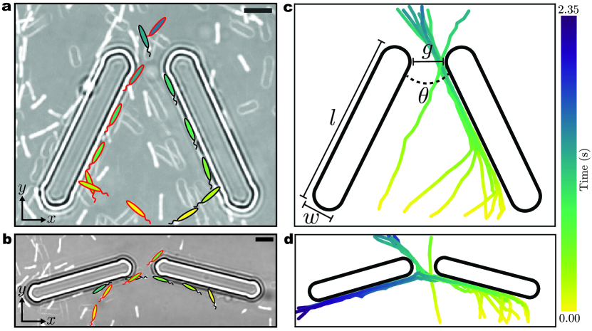
Figure 1: Bacterium-wall interaction in bacterial rectification. Superimposed time-series showing rectification of two prototypical E. coli by funnel walls at $\theta=50\degree$ (a) and $150\degree$ (b). Stylized ellipsoids placed on top of actual cell bodies are color-coded to show time evolution, where the black and red outlines distinguish the two different bacteria. Representative bacterial trajectories for $\theta=50\degree$ (c) and $150\degree$ (d). For clarity, only bacteria hitting the right funnel wall are shown. For the obtuse $\theta$, when a bacterium reaches the funnel tip, its head position on the opposite wall of the funnel and the wobble angle at the moment of collision dictate one of the two outcomes. If the tip of its body is above the lower boundary of the opposite wall, the bacterium goes up in the $+y$ direction and is rectified (e.g. the bacterium approaching the funnel from the left in b). If the tip of its body is below the lower boundary, the bacterium goes down in the $-y$ direction and is not rectified (e.g. the bacterium approaching from the right in b). The geometrical parameters of the funnel are indicated in c. Scale bars are 5 $\mu$m.

Because of its potential applications in biotechnology such as cell sorting and trapping [18, 19, 20, 21], micro-patterning [18] and spontaneous pumping [18], the rectification of the motion of active particles using fixed asymmetric structures has been extensively studied both numerically [22, 23, 24, 25] and in experiments [18, 26, 27, 25, 28, 29, 30, 21, 26]. Inspired by seminal experiments of Austin, Chaikin, and co-workers on swimming bacteria [18], most of these studies adopted microfluidic devices with an array of funnel-shaped obstacles, which spontaneously induce a concentration difference of active particles between the two sides of the array, starting from a uniform active bath [16, 22, 23, 24, 25, 26, 27, 28]. Nevertheless, despite extensive research, important questions such as the optimal funnel geometry and the maximum rectification efficiency still remain unanswered. Thus, beyond elucidating the fundamental non-equilibrium thermodynamic relations, the second objective of our study is to address the practical issue of the optimal rectification of bacterial motion.

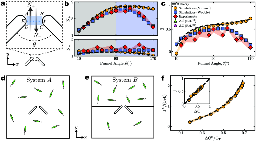
Figure 2: Local fluxes and rectification efficiency. a, Schematic showing bacterial fluxes through a funnel tip of angle $\theta$. $EF$ is the center line of the region of interest $ABCD$. ${N}_{+}$ and ${N}_{-}$ indicate normalized number of particles crossing $EF$ per unit line and time in the $+y$ and $-y$ directions, respectively. b, ${N}_{+}$ and ${N}_{-}$ as a function of $\theta$ with the acute and obtuse $\theta$ regions shaded differently. c, Rectification efficiency, quantified by the normalized flux difference per particle, $\widetilde{J}$, as a function of $\theta$. Data from previous experiments [18, 26] are extracted for comparison based on Eq. (2). The dashed black lines in b and c are predictions from Eqs. (16) and (17). To mimic experimental funnel geometry, we adopt round-cornered funnel walls for wobbling simulations (see Fig. 1 and Extended data Fig. 1a). d, Schematic of our system (System “$A$”) with finite number flux $J$ at steady state. e, Schematic of System “$B$” considered in previous studies [18, 26, 27, 28, 25, 22, 23, 24], leading to a finite concentration difference $\Delta C$ between the $+y$ and $-y$ regions at steady state. f, Comparison of $J/(C_{T}k)$ measured from d and $\Delta C/C_{T}$ measured from e for each corresponding $\theta$. The inset shows the same relation in terms of normalized variables $\widetilde{J}$ and $\Delta\widetilde{C}$. The dashed black line is the prediction of Eq. (2). All shaded regions denote measurement standard deviations.

.1 Setup

We inject a dilute suspension of Escherichia coli (E. coli) in a quasi-two-dimensional (2D) polydimethylsiloxane (PDMS) microfluidic chamber containing isolated funnel-shaped obstacles with angles ($\theta$), length ($l$), width ($w$) and gap ($g$) (Fig. 1c, see Fig. 2d for a schematic representation). Unless stated otherwise, $l/g=6$ and $w/g=1$ in our study. The trajectories of the bacteria and the interaction between bacteria and wall are then imaged via optical microscopy (Fig. 1 and Supplementary Information (SI) Sec. I).

Away from funnel walls, free-swimming E. coli exhibit the classic “run-and-tumble” motion [31]. In the run phase, the trajectory of the bacterium is helical, which manifests as wobbling of the bacterial body under the 2D projection of optical microscopy [32, 33]. Independent of the angle of incidence, a bacterium always re-aligns and moves parallel to the funnel walls after hitting the walls (Figs. 1a and c) [18]. We incorporate the surface aligning trait of E. coli in our minimal simulations, where we model bacteria as point non-interacting particles performing run-and-tumble motions (SI Sec. II.A) [24].

.2 Fluxes

Our locally-defined system of interest is a small region ABCD at the funnel tip (Fig. 2a). The number of bacteria leaving the center-line EF of ABCD per unit time and length in the $+y$ $(-y)$ direction, normalized by the same quantity from a region far from the funnel gap, is denoted by ${N}_{+}$ (${N}_{-}$). Figure 2b shows ${N}_{+}$ and ${N}_{-}$ as a function of $\theta$. Since $w\approx g$ is small compared with $l$, reverse rectification is not pronounced, leading to a nearly constant ${N}_{-}\approx 1$ (Fig. 2b). In contrast, ${N}_{+}$ shows a non-monotonic trend with increasing $\theta$. Minimal simulations show reasonable agreement with experiments for acute $\theta$ but deviate from experiments when $\theta$ is obtuse (Fig. 2b). Accordingly, we discuss our results in these two regimes separately.

Figure 3: Breaking of local time-reversal symmetry. a, Schematic showing the three discrete states ${0,+v,-v}$ assigned to the region $ABCD$ at the funnel tip. Bacteria are depicted as ellipsoids without flagella to highlight that the orientation of bacteria is not tracked. The lower panels show the time-reversed counterpart of the upper panels. Specifically, a local state, $s$, is distinguished as follows: $s=0$ when a particle is absent and $s=+v$ $(-v)$ if a particle is present and is moving in the $+y$ $(-y)$ direction. The time-reversed sequence of states is obtained from the time-forward sequence by changing $+v$ to $-v$ and vice versa ($s=0$ states remain invariant under time reversal). The orientation of bacteria—an even variable under time reversal—and therefore the orientation irreversibility is not tracked, which is trivially present with or without the funnel rectifier because of the self-propulsion of bacteria [34]. The time-forward trajectory, X, is filtered by removing all the $s=0$ states since they remain invariant under time reversal. This filtering retains the essential irreversibility (Extended Data Fig. 4c, SI Sec. III). b, Time irreversibility $\sigma$ as a function of funnel angle $\theta$. c, $\sigma$ as a function of normalized flux difference per particle, $\widetilde{J}$. The inset shows a log-log plot of the same curve. The dashed black lines in b and c are predictions from Eq. (4). All shaded regions denote measurement standard deviations.

Acute $\theta$. As more bacteria can enter a funnel of wider opening, ${N}_{+}$ increases with $\theta$ (Fig. 2b). The agreement between our minimal simulations and experiments for acute $\theta$ has two important implications. First, even though bacteria-wall interactions are governed by complex steric and near-field hydrodynamic forces [35, 36, 37, 38], from the perspective of rectification such complex interactions can nevertheless be effectively condensed into one simple rule: E. coli reorient themselves parallel to the wall after a collision. Such a simple rule has been ignored in the majority of numerical studies on bacterial rectification [22, 23, 25] with notable exceptions [24]. Second, the rectification efficiency, quantified by the normalized flux per particle, $\widetilde{J}\equiv({N}_{+}-{N}_{-})/({N}_{+}+{N}_{-})$, increases monotonically with $\theta$ (Fig. 2c).

Obtuse $\theta$. The system shows a more complex behavior when $\theta>90\degree$, a regime that has not been explored heretofore. Figure 2b, shows a maximum in $N_{+}$ at $\theta\equiv\theta_{\max}\approx 120\degree$ in both minimal simulations and experiments. Such a non-monotonic trend, in combination with the nearly constant ${N}_{-}$, results in the maximum rectification efficiency at $\theta=\theta_{\max}$ (Fig. 2c). As $\theta$ increases, there is an increase in both the number of bacteria entering the funnel and those turning back down in the $-y$ direction after hitting the interior funnel walls. The competition between these two effects gives rise to the non-monotonic trend in $N_{+}$.

This discrepancy between experiments and minimal simulations can be traced down to bacterial wobbling as illustrated in Figs. 1b and d, where it can be seen that a fraction of bacteria turn back in the $-y$ direction after reaching the funnel tip, leading to a reduction of ${N}_{+}$. Since the threshold amount of wobbling needed for bacteria to turn back decreases with $\theta$, the wobbling effect becomes more evident as $\theta$ increases. To explicitly demonstrate the effect of wobbling on bacterial rectification, we incorporate bacterial wobbling in our minimal simulations (Fig. 2b, SI Sec. II.B), which then quantitatively match our experiments.

Despite extensive experimental and numerical studies on the rectification of active particles using funnel-shaped obstacles [18, 26, 27, 28, 25, 22, 23, 24], an analytical model of the process remains elusive. Here, combining a universal distribution of self-propulsion directions of particles at the funnel gate with geometrical considerations, we develop a mechanical model of rectification, giving analytical expressions for ${N}_{+}(\theta,l,g)$ and ${N}_{-}(\theta,l,g)$ (Eqs. (16), (17), Methods). Without fitting parameters, Eqs. (16) and (17) quantitatively predict ${N}_{+}(\theta)$ and ${N}_{-}(\theta)$ in minimal simulations, and in experiments at acute angles when bacterial wobbling is unimportant (Fig. 2b).

Our mechanical model allows us to derive a generalized mass transfer relation for bacterial rectification, relating instantaneous bacterial number flux, $J(t)$, to two opposing driving forces. The first contribution comes from the concentration difference, $\Delta C(t)$, between the two sides ($+y$ and $-y$) of the chamber, and the second is due to the funnel rectifier, whose influence can be mapped to an effective concentration difference $\Delta C^{\mathrm{eff}}(t)$, giving (Methods),

$$J(t)=-k\left[\Delta C(t)+\Delta C^{\mathrm{eff}}(t)\right].$$ (1)

Here, $k$ is the mass transfer coefficient linking flux to an externally applied concentration difference, which is independent of rectification and determined using a system without a funnel rectifier (Extended Data Fig. 3a, c, d).

We first apply Eq. (1) to a previously well-explored system in which the funnel is embedded in a partition (or an array of funnels) separating the chamber into two regions [18, 26, 27, 28, 25, 22, 23, 24]. This system (Fig. 2e), which we label as System $B$, leads to a concentration difference, $\Delta C^{B}(t)$, across the two sides of the chamber, which is predicted exactly by Eq. (1) (Eq. (31), Methods, Extended Data Fig. 3b, SI Sec. II.E). At steady state, the two forces in Eq. (1) balance out, and the flux $J^{B}=0$.

In our system (System $A$, Fig. 2d), at steady state, a finite flux $J^{A}$ is sustained at the funnel tip by the second term in Eq. (1) alone, whereas the concentration difference vanishes along with the first term. Equation (1), when applied independently to both Systems $A$ and $B$, enables us to connect the bacterial number flux, $J^{A}$, produced at the funnel tip in our system, with the concentration difference, $\Delta C^{B}$, measured at steady state across the funnels in previous studies [18, 26, 27, 28, 25, 22, 23, 24],

$$J^{A}=kR\Delta C^{B}.$$ (2)

Here, $R=({N}_{+}+{N}_{-})/2$ is a correction factor due to the funnel rectifier and is determined by the mechanical model (Eqs. (16) and (17)). In terms of the normalized flux per particle, $\widetilde{J}\equiv\widetilde{J}^{A}$, Eq. (2) becomes $\widetilde{J}={\Delta C^{B}}/{C_{T}}\equiv\Delta\widetilde{C}$, where $C_{T}$ is the total concentration of the chamber (Eq. (34), Methods). The quantitative relation between our system (Fig. 2d) and the system in previous studies (Fig. 2e) [18, 26, 27, 28, 25, 22, 23, 24] can thus be formally established (Fig. 2f, SI Sec. II.E).

Equation (2) thus allows us to compare our experiments with previous studies [18, 26], showing good agreement (Fig. 2c). Importantly, these previous studies on bacterial rectification fixed the angle, $\theta=60\degree$, which, as we show, does not correspond to the maximum rectification efficiency (Fig. 2c), cf. $\theta_{\max}\approx 120\degree$ from our experiments and $\theta_{\max}\approx 119\degree$ from our theory when reverse rectification is not pronounced ($N_{-}(\theta)\approx$ constant) (Methods).

.3 Time irreversibility

Irreversible processes are accompanied by a loss of heat to the environment quantified by a positive EPR, $\dot{S}>0$—a clear signature of TRSB [39]. For a system in non-equilibrium steady state (NESS), the Kullback-Leibler divergence (KLD), $\sigma$, between the probability of observing a time-forward trajectory (X) of a subset of degrees of freedom (DOFs) and its time-reversed counterpart ($\textbf{X}^{\textbf{R}}$) bounds $\dot{S}$ from below [40, 41, 42, 43, 39, 44, 45, 46, 25, 41],

$$\dot{S}\geq\frac{k_{B}}{\tau}\sigma=\frac{k_{B}}{\tau}\biggl{\langle}\ln\frac{P[\textbf{X}]}{P[\textbf{X}^{\textbf{R}}]}\biggl{\rangle},$$ (3)

where $k_{B}$ is the Boltzmann constant, $\tau$ is the sampling interval, and $P[\textbf{X}]$ and $P[\textbf{X}^{\textbf{R}}]$ are the probability density functions of the time-forward and backward dynamics, respectively. $\langle\cdot\rangle$ denotes average over $P[\textbf{X}]$. When applied independently to different DOFs and spatial positions [25], Eq. (3) can be used to obtain information about DOFs and spatial positions that are dominantly irreversible.

To quantify the local time irreversibility at the funnel tip, we measure the $y$-component of position and velocity of bacteria in region ABCD to obtain a local state, $s$, of the system at a given time (Fig. 3a). Here, we account only for the direction of velocity, assuming the magnitude remains constant on average. At low concentrations, the events of bacteria crossing the funnel tip are independent (Extended data Fig. 4a, b, SI Sec. III).

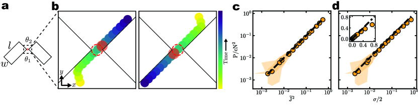
Figure 4: Extractable work from bacterial rectification in an ideal scenario. a, Schematic of a system for measuring extractable work. A funnel rectifier with symmetric angles ($\theta_{1}=\theta_{2}=90\degree$) is immersed in a bath of bacteria with a harmonically trapped colloid (shown in red) placed at the tip. b, Superimposed time-series trajectories of bacteria approaching the colloid along the $+y$ (left figure) and $-y$ (right figure) directions. The dotted red lines denote the rest position and the filled red circles denote the maximum displacement of the colloid. Comparing normalized extractable power, $P/cN^{2}$, with normalized flux difference per particle, $\widetilde{J}$ (c), and time-irreversibility (KLD), $\sigma$ (d). The black dashed lines are the prediction of Eq. (6). Different bacterial fluxes are generated by varying the funnel aspect ratio $l/w$. The inset of (d) shows a linear scale plot of $P/cN^{2}$ versus $\sigma/2$. All shaded regions denote measurement standard deviations.

From the independence of the crossing events, $P[\textbf{X}]$ and $P[\textbf{X}^{\textbf{R}}]$ should follow Bernoulli distributions with the probability parameters $p={N}_{+}/({N}_{+}+{N}_{-})$ and ${N}_{-}/({N}_{+}+{N}_{-})$, respectively. Eq. (3) then allows us to calculate $\sigma$ as,

$$\sigma=\frac{{N}_{+}}{{N}_{+}+{N}_{-}}\ln\left(\frac{{N}_{+}}{{N}_{-}}\right)+\frac{{N}_{-}}{{N}_{+}+{N}_{-}}\ln\left(\frac{{N}_{-}}{{N}_{+}}\right).$$ (4)

Finally, substituting ${N}_{+}(\theta)$ from Eq. (16) and ${N}_{-}(\theta)$ from Eq. (17) (Methods), we obtain an analytical expression for $\sigma(\theta)$. We also measure $\sigma$ directly from filtered X and $\textbf{X}^{\textbf{R}}$ using recently introduced KLD estimators [25], which quantitatively match the prediction of Eq. (4) (Extended data Fig. 4c, d, SI Sec. III).

Figure 3b shows that $\sigma$ increases monotonically with $\theta$ for bacteria without wobble. For wobbling bacteria, instead, we observe a non-monotonic trend with a peak around $\theta\approx 120\degree$. By comparing Figs. 2c and 3b, it is apparent that $\sigma$ and $\widetilde{J}$ follow quantitatively similar trends and peak at the same $\theta=\theta_{\max}$, verifying that the time irreversibility of the system is intimately coupled to local fluxes.

The quantitative relation between the degree of TRSB in non-equilibrium DOFs (here position and momentum) and the presence of fluxes in those DOFs (here mass and momentum fluxes) can be analyzed further. Figure 3c shows $\sigma$ as a function of $\widetilde{J}$. $\sigma$ increases monotonically with $\widetilde{J}$, verifying the coupling between the local time irreversibility and the local mass (and momentum) flux at the funnel tip. More importantly, bacteria with or without wobble show the same behavior, indicating that the quantitative relation between $\sigma$ and $\widetilde{J}$ is universal, independent of the type of active particles (Fig. 3c).

In the limit of small fluxes, $\widetilde{J}\rightarrow 0$, we find $\sigma\propto\widetilde{J}^{2}$ (Fig. 3c inset), a relation that is also obtained from the Taylor expansion of Eq. (4). This is reminiscent of the classic result of linear irreversible thermodynamics, where the quadratic relation is derived under the assumptions of linearity between flux and its conjugate thermodynamic force and of local thermodynamic equilibrium [5]. In contrast, Eq. (4) assumes neither a system near equilibrium in the linear regime nor that the flux is generated by thermodynamic forces. When the flux is large, the quadratic relation does not hold with $\sigma$ increasing faster than $\widetilde{J}^{2}$ (Fig. 3c inset).

When multiplied by $k_{B}T/\tau$, $\sigma$ estimates the rate at which an irreversible system dissipates heat when connected to a thermal reservoir at temperature $T$ (or equivalently, the energetic cost of maintaining a NESS). Thus, our measurement of $\sigma$ gives the lower bound on the extra energy needed to maintain a steady flux of bacteria ($\sim 300\,k_{B}$ s^-1), in addition to the chemical fuel required for bacterial motility (due to orientation irreversibility present with or without a funnel rectifier). While it might seem that rectification through passive, fixed obstacles has no active energetic cost, a non-zero $\sigma$ clearly demonstrates that energy is indeed required for rectifying bacteria. The extra energy includes but is not limited to the energetic cost of reorientation (flagellar (re)bundling) and the increased dissipative cost of bacterial motion near boundaries compared to bulk.

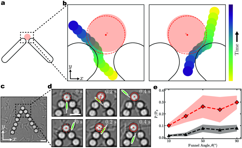
Figure 5: Extractable work from bacterial rectification in a non-ideal scenario. a, Schematic of a system showing a colloid (red) trapped harmonically at the tip of a funnel rectifier. The colloid cannot have large displacements in the $-y$ direction due to the constraint of the wall. b, Superimposed time-series trajectories of bacteria approaching the colloid along the $+y$ (left figure) and $-y$ (right figure) directions. The dotted red lines denote the rest position and the filled red circles denote the maximum displacement of the colloid. c, Experimental realization of the system introduced in (a), where the funnel “wall” is composed of colloids harmonically trapped by optical tweezers. The funnel angle is $\theta=50\degree$. The tip colloid is held weakly compared to wall colloids. d, Time series showing typical bacterium-colloid interactions where the tip colloid (the solid red circle) is displaced in the $+y$ direction by the bacteria irrespective of their approaching directions. Stylized ellipsoids are superimposed on cell bodies for clarity. The positions of the colloid at $t=0$ s are indicated by dashed red lines. Scale bars are 5 $\mu$m. e, Extractable power $P$ as a function of $\theta$. $P$ is normalized by the power of a single bacterium $P_{0}$. Red diamonds are from experiments and black triangles are the prediction of Eq. (6) with experimental fluxes as input. Shaded regions denote measurement standard deviations.

.4 Extractable work

Finally, we investigate the extractable work from bacterial rectification. We first examine the relation between fluxes, time irreversibility, and extractable work in an ideal scenario, where an analytical solution can be obtained. Particularly, we trap a colloid in a harmonic potential at a symmetric funnel tip with $\theta_{1}=\theta_{2}=90\degree$ (Fig. 4a). The colloid is weakly coupled to bacterial motion such that the bacterial flux at the funnel tip remains the same with or without the trapped colloid, as quantified by comparing the flux, $\widetilde{J}$, in the two cases (Extended data Fig. 5). It should be emphasized that our system is different from autonomous engines studied previously, where asymmetric objects arrest active particles over long periods of time and qualitatively change particle fluxes [10, 11, 9, 15, 13].

Figure 4b shows typical bacterium-colloid interactions in this ideal scenario for bacteria coming from both $+y$ and $-y$ directions, where a bacterium pushes the colloid along its self-propulsion direction when passing through the tip. We measure the time-averaged $y$-position of the colloid, $y_{c}$, which is non-zero due to a net mass (and momentum) flux in the $+y$ direction. Even though the motion of the colloid is stochastic, rectified bacterial motion provides a non-zero time-averaged driving force $F=Ky_{c}$ against the pulling of the harmonic trap, which allows for work extraction when the force is coupled to an external load. Here, $K$ is the elastic constant of the trap. In the linear regime, we can write (Methods),

$$P=\frac{F^{2}}{4\mu},$$ (5)

where $\mu$ is the mobility of the colloid and $P$ is the extractable power.

From Eq. (5) and the relations between $F$, $\widetilde{J}$ and $\sigma$ (Methods), we reach a generic relation linking extractable work, particle flux, and time irreversibility,

$$P=cN^{2}\widetilde{J}^{2}\underset{\widetilde{J}\to 0}{=}cN^{2}\frac{\sigma}{2},$$ (6)

where $N$ is the total number of bacteria crossing the funnel tip and $c$ is a computable system-dependent constant (Eq. (25), Methods). The interrelationship of Eq. (6) holds under two general assumptions: (i) weak coupling, meaning that $\widetilde{J}$ remains the same with or without the work-measuring or work-extracting mechanism; (ii) only one irreversible DOF is coupled to work extraction. Other DOFs are either uncoupled or if coupled, reversible. Numerical simulations of the ideal scenario show excellent agreement with Eq. (6) (Figs. 4c and d, SI Sec. II.C), confirming the quantitative relation between local flux ($\widetilde{J}$), time irreversibility ($\sigma$) and extractable power ($P$).

Eq. (6) illustrates that an autonomous work-extracting mechanism leverages the spontaneous fluxes generated in a time-irreversible system. For a system in a NESS, the departure from equilibrium can be quantified in terms of time-irreversibility and fluxes: a system farther away from equilibrium is more irreversible and has stronger fluxes [47, 48]. Thus, Eq. (6) reveals that more power can be harnessed from systems farther away from equilibrium. Another consequence of Eq. (6) is that if all the DOFs in a spatial region are locally reversible, $P$, $\widetilde{J}$ and $\sigma$ would all simultaneously be zero, a result that has been found recently [25].

Is there a way to extract more work from a time-irreversible system than predicted for the ideal scenario? This can indeed be achieved by relaxing the assumptions in the derivation of Eq. (6). Figure 5a shows one possible way to relax the second assumption by introducing a slight modification to the system in Fig. 4a, where the position of the colloid is chosen such that the funnel walls prevent it from having large displacements in the $-y$ direction (Fig. 5a, SI Sec. II.D). A typical bacterium-colloid interaction in this new scenario sees the colloid moving in the $+y$ direction irrespective of the direction of bacterial swimming (Fig. 5b). Thus, the interaction between the colloid and downward-moving bacteria is rectified, which retrieves the lost work in the ideal scenario and increases the total extractable work. While this modified system still obeys the weak coupling assumption, it does not follow the second assumption under which Eq. (6) was derived. The force exerted by the wall on the tip colloid prevents the colloid to move freely in the $-y$ direction and therefore acts as an additional irreversible DOF coupled to the colloid.

To demonstrate the possibility of experimentally measuring extractable work from bacterial rectification, we design an experiment that realizes the non-ideal scenario discussed above. Specifically, our experiment consists of a funnel-shaped “wall” of spherical colloids in a dilute bacterial bath (Fig. 5c). The wall particles are held strongly by harmonic traps made using optical tweezers, whereas the colloid at the tip is loosely held to satisfy the weak coupling condition for work extraction (SI Sec. I.C). Figure 5d shows typical bacterium-colloid interactions in experiments, which are qualitatively similar to the scenario in Fig. 5a. As shown in Fig. 5e, experimentally measured $P$, normalized by the power of a single bacterium ($P_{0}\approx 1.8\times 10^{-18}$ W, SI Sec. I.C), is non-zero and increases with $\theta$ as more bacteria are rectified at large $\theta$. More importantly, the power in this non-ideal scenario is consistently higher than that predicted by Eq. (6), agreeing with our analysis.

Thus, our study combining experiments, simulations, and theory has two important contributions. First, we provided a quantitative microscopic understanding of bacterial rectification, revealing an optimal funnel geometry resulting from a complex interplay between bacterium-wall interactions and bacterial wobbling. Second, the interrelationship between local fluxes, time irreversibility, and extractable work was uncovered in a living system far from equilibrium, providing a useful guideline for systematically harnessing work from non-equilibrium systems.

I Methods

II Theory

II.1 Mechanical model of bacterial rectification

We develop a mechanical model of bacterial rectification, which predicts the dependence of bacterial fluxes on the geometry of the funnel (Fig. 1). In the model, we assume that (i) the particles are point-like, non-interacting, and undergo run-and-tumble without wobbling; (ii) the run length of particles is much longer than the funnel length, $l_{r}\gg l$; and (iii) the gap of the funnel is much smaller than the funnel length, $g\ll l$. Although the model considers sharp-cornered rectangular funnels with straight walls, the model prediction agrees well with experiments of round-cornered rectangular funnels when the funnel angle $\theta<90^{\circ}$.

The number flux in 2D is defined as the net flow of the number of particles per unit length and time. The line of interest here is the line “EF” at the funnel tip (Fig. 2a). Since we are only interested in the number of bacteria crossing $EF$ and not the angle of crossing relative to $EF$, the flux we define is a coarse-grained flux. We denote ${N}^{{}^{\prime}}_{+}$ $({N}^{{}^{\prime}}_{-})$ the number of particles crossing $EF$ in the $+y$ $(-y)$ direction per unit length and time. The flux through $EF$ can then be written as $({N}^{{}^{\prime}}_{+}-{N}^{{}^{\prime}}_{-})$. Furthermore, we denote ${N}_{+}^{o}$ (${N}_{-}^{o}$) the number of particles moving in $+y$ ($-y$) direction per unit length and time in the bulk (far from the funnel gap).

We start by modeling ${N}^{{}^{\prime}}_{+}$ as the product of (i) the number of particles arriving at the funnel opening $GH$ and moving in the $+y$ direction, ${N}_{+}^{o}L$, and (ii) the fraction of particles that continue to move in the $+y$ direction after a collision with the inside of the funnel walls, $\psi$ (Extended Data Fig. 2a). Thus, from the conservation of particles, ${N}^{{}^{\prime}}_{+}g={N}_{+}^{o}L\psi$, where $L=2l\sin(\theta/2)+g$ is the length of the funnel opening $GH$ (Extended Data Fig. 2a). As ${N}_{+}^{o}\sim\phi v$, where $\phi$ is the number density and $v$ is the self-propulsion speed of particles, we define a normalized particle flux ${N}_{+}$,

$${N}_{+}\equiv\frac{{N}^{{}^{\prime}}_{+}}{{N}_{+}^{o}}=\frac{L}{g}\psi=\left(2\frac{l}{g}\sin\frac{\theta}{2}+1\right)\psi,$$ (7)

which removes the trivial dependencies on $\phi$ and $v$. ${N}_{+}=1$ at any arbitrary line segment chosen in the bulk and at $GH$.

To calculate $\psi$, we first determine the probability distribution of the self-propulsion angle of particles, $\alpha$, crossing a horizontal line segment in the bulk away from the funnel and moving in the $+y$ direction, $P(\alpha)$. Since the motion of particles is random, it may intuitively seem that $P(\alpha)$ should be a uniform distribution. This, however, is not the case because of two factors, which we illustrate below. Consider a case where $n$ particles initially start at a self-propulsion angle $\alpha$ spatially uniformly distributed along a horizontal line segment $WX$, which lies slightly below the horizontal line segment of interest $YZ$ and has the same length as $YZ$ (Extended Data Fig. 2b). If all particles continue to move in straight lines for a long enough time, $n\sin\alpha$ particles would be able to cross $YZ$. This can easily be seen by rotating the coordinate axis by an angle $(\pi/2-\alpha)$ anti-clockwise, making the particles move vertically in the transformed coordinate system (Extended Data Fig. 2b). The number of particles crossing the transformed line $Y^{\prime}Z^{\prime}$ is proportional to the projection of $Y^{\prime}Z^{\prime}$ onto $YZ$, or $n\sin\alpha$ (Extended data Fig. 2b). This is the first factor arising due to a geometrical reason and is valid when the observation time is long. However, for a finite observation time, the number of particles starting from $YZ$ and reaching $WX$ is proportional to the magnitude of the $y-$component of their self-propulsion velocity, $v\sin\alpha$. When combined with the geometric factor above, this second factor due to particle kinematics gives the number of particles starting from $YZ$ and reaching $WX$, which is $\sim\sin^{2}\alpha$. Noting that $\alpha\in[0,\pi]$, we can write the $P(\alpha)$ as a raised cosine distribution supported on the interval $[\mu_{0}-\sigma_{0},\mu_{0}+\sigma_{0}]$ with the mean $\mu_{0}=\pi/2$ and $\sigma_{0}=\pi/2$,

$$P(\alpha)=\frac{2}{\pi}\sin^{2}\alpha=\frac{1}{\pi}\left[1-\cos(2\alpha)\right].$$ (8)

Equation (8) can be rewritten as a standard raised cosine distribution $P(\alpha_{norm})$ having parameters $\mu_{0}=0,\,\sigma_{0}=1$ by normalizing $\alpha$ as $\alpha_{norm}=(\alpha-\pi/2)/(\pi/2)$. Extended Data Figure 2e shows $P(\alpha_{norm})$ for varying funnel angles $\theta$ from minimal simulations, which agree well with the standard raised cosine distribution, as predicted by Eq. (8). Going forward, for the $\psi$ calculation, we divide our discussion of the parameter space $\theta\in(0,\pi)$ into two regimes, i.e., acute $\theta$ ($0<\theta\leq\pi/2$) and obtuse $\theta$ ($\pi/2<\theta<\pi$).

Acute $\theta$. Once a particle reaches the funnel gate, it goes up ($+y$) after a collision with the inside of funnel walls only if $\alpha\in[\theta/2,\,\,\pi-\theta/2]$ (Extended Data Fig. 2c). Importantly, this geometric consideration is valid irrespective of the location of the particle at the funnel gate. $\psi$ can then be written as the fraction of $P(\alpha)$ that falls within the range $[\theta/2,\,\,\pi-\theta/2]$,

$$\psi=2\int\limits_{\frac{\pi}{2}}^{\pi-\frac{\theta}{2}}P(\alpha)\,d\alpha=\frac{1}{\pi}(\pi-\theta+\sin\theta)\equiv A(\theta),$$ (9)

where we have used the fact that $P(\alpha)$ is symmetric around $\alpha=\pi/2$. Combining Eqs. (7) and (9), we find $N_{+}$ for acute angles,

$${N}_{+}=\left(2\frac{l}{g}\sin\frac{\theta}{2}+1\right)A(\theta).$$ (10)

Obtuse $\theta$. We consider only the left half of the funnel gate since the funnel is symmetric around the $y$-axis (Extended Data Fig. 2d). We divide the half-funnel opening $GH^{\prime}$ into two segments $GG^{\prime}$ and $G^{\prime}H^{\prime}$, which have lengths $l[\sin(\theta/2)-\cot(\theta/2)\cos(\theta/2)]$ and $l\cot(\theta/2)\cos(\theta/2)$, respectively (Extended Data Fig. 2d). For a particle landing on $GH^{\prime}$, the geometric consideration developed previously for acute $\theta$ applies as well, which is independent of the position of the particle. For a particle landing on $GG^{\prime}$, however, the particle also goes up after a collision if $\alpha\in[\theta/2-\beta,\,\,\theta/2]$, where $\beta\in[0,\,\,\theta-\pi/2]$ depends on the position of the particle (Extended Data Figs. 2c, d). Note that this “additional fraction” $\psi^{\prime}$ of particles going through the gap was neither present in the acute $\theta$ regime nor for the region $G^{\prime}H^{\prime}$ in the obtuse $\theta$ regime. To estimate the additional contribution $\psi^{\prime}$ from the segment $GG^{\prime}$, we first find the average of $\beta$, $\beta_{avg}$,

$$\begin{split}\beta_{avg}&=\int\limits_{\pi-\frac{\theta}{2}}^{\frac{\pi}{2}+\frac{\theta}{2}}\beta P(\beta)\,d\beta=\int\limits_{\pi-\frac{\theta}{2}}^{\frac{\pi}{2}+\frac{\theta}{2}}\beta\frac{1}{\pi}(1-\cos(2\beta))\,d\beta\\ &=\left(\frac{3}{4}+\frac{\sin\theta}{2\pi}\right)\left(\theta-\frac{\pi}{2}\right)+\frac{\cos\theta}{2\pi},\end{split}$$ (11)

where we use the condition that a particle is equally probable to land anywhere on $GG^{\prime}$. $\psi^{\prime}$ is then,

$$\psi^{\prime}=\int\limits_{\pi-\frac{\theta}{2}}^{\pi-\frac{\theta}{2}+\beta_{avg}}P(\alpha)\,d\alpha=\int\limits_{\pi-\frac{\theta}{2}}^{\pi-\frac{\theta}{2}+\beta_{avg}}\frac{1}{\pi}[1-\cos(2\alpha)]\,d\alpha=\frac{1}{\pi}\left[\beta_{avg}-\sin\beta_{avg}\cos(\theta-\beta_{avg})\right].$$ (12)

Combining Eq. (12) with the usual fraction of particles going up from the segment $GH^{\prime}$ (Eq. (9)) and noting that the fractional length of segment $GG^{\prime}$ compared to the half funnel gate $GH^{\prime}$ is $1-\cot^{2}(\theta/2)$, we achieve $\psi$ for obtuse $\theta$,

$$\psi=A(\theta)+\frac{1}{\pi}\left(1-\cot^{2}\frac{\theta}{2}\right)\left[B(\theta)-\sin(B(\theta))\cos(\theta-B(\theta))\right],$$ (13)

where $B(\theta)$ is given as,

$$B(\theta)\equiv\beta_{avg}=\left(\frac{3}{4}+\frac{\sin\theta}{2\pi}\right)\left(\theta-\frac{\pi}{2}\right)+\frac{\cos\theta}{2\pi}.$$ (14)

Combining Eq. (13) with Eq. (7), we have ${N}_{+}$ for the obtuse $\theta$ regime as,

$${N}_{+}=\left(2\frac{l}{g}\sin\frac{\theta}{2}+1\right)\left[A(\theta)+\frac{1}{\pi}\left(1-\cot^{2}\frac{\theta}{2}\right)\left(B(\theta)-\sin(B(\theta))\cos(\theta-B(\theta))\right)\right].$$ (15)

Finally, combining Eqs. (10) and (15), we get

$$N_{+}=\begin{dcases}\left[2\frac{l}{g}\sin\frac{\theta}{2}+1\right][A(\theta)]&\forall\;\theta\leq\frac{\pi}{2}\\[10.0pt] \begin{aligned} \left[2\frac{l}{g}\sin\frac{\theta}{2}+1\right]&\left[A(\theta)+\frac{1}{\pi}\left(1-\cot^{2}\frac{\theta}{2}\right)(B(\theta)-\sin B(\theta)\cos(\theta-B(\theta)))\right]\end{aligned}&\forall\;\theta\geq\frac{\pi}{2}.\end{dcases}$$ (16)

The downward particle flux ${N}_{-}$ can be written by simply replacing $\theta$ with $\pi-\theta$ and $l$ by $w$ (Extended Data Fig. 2a), which gives

$${N}_{-}=\begin{dcases}\left[2\frac{w}{g}\cos\frac{\theta}{2}+1\right]\left[A(\pi-\theta)+\frac{1}{\pi}\left(1-\tan^{2}\frac{\theta}{2}\right)(B(\pi-\theta)+\sin B(\pi-\theta)\cos(\theta+B(\pi-\theta)))\right]&\forall\;\theta\leq\frac{\pi}{2}\\[10.0pt] \left[2\frac{w}{g}\cos\frac{\theta}{2}+1\right][A(\pi-\theta)]&\forall\;\theta\geq\frac{\pi}{2}.\end{dcases}$$ (17)

In the derivation of ${N}_{+}$ and ${N}_{-}$ above, we do not consider particles that directly go through $EF$ without interacting with the inside of funnel walls. While the number of such particles vanishes when $l/g\gg 1$ (and $w/g\gg 1$) making our analytical expressions of ${N}_{+}$ (and ${N}_{-}$) exact in that limit, our theoretical predictions are nevertheless reasonable even for modestly finite funnel gaps when $l/g\approx 1$ (or $w/g\approx 1$). Extended Data Figure 2f compares predictions from Eqs. (16) and (17) to numerical simulations, showing good agreement for experimentally relevant value of $l/g=6$ and $w/g=1$ and reasonable agreement even for modestly wide funnel gaps ($l/g=w/g=1$). Additionally, despite being derived for the sharp-cornered funnel, our mechanical model nevertheless correctly predicts ${N}_{+}$ and ${N}_{-}$ for the round-cornered funnel when $\theta<135\degree$ (Extended Data Fig. 1c).

What is the funnel angle corresponding to maximal rectification efficiency, as quantified by $\widetilde{J}(\theta)\equiv({N}_{+}-{N}_{-})/({N}_{+}+{N}_{-})$? For $l/g=6$, $w/g=1$ and $\theta\in(0\degree,180\degree)$, $\widetilde{J}$ increases monotonically with $\theta$, as predicted by the mechanical model (Eqs. (16) and (17)) and confirmed by minimal simulations (Fig. 2a, c). Experiments and simulations with wobbling bacteria show a nearly constant $N_{-}$, independent of $\theta$ (Fig. 2b). Under this assumption, it suffices to maximize $N_{+}$ to get the optimum $\widetilde{J}$ for experiments and simulations with wobbling bacteria. Maximizing $N_{+}$ given by Eq. (16) yields $\operatorname*{argmax}_{\theta}\widetilde{J}(\theta)=119.175\degree$, in good agreement with experiments and wobble simulations ($\theta\approx 120\degree$) (Fig. 2c).

II.2 Relation between fluxes and time-irreversibility

The KLD, $\sigma$, between two Bernoulli distributions with parameters $p$ and $1-p$ is given by:

$$\sigma=p\ln\left(\frac{p}{1-p}\right)+(1-p)\ln\left(\frac{1-p}{p}\right).$$ (18)

Since the probability density functions for time-forward and reverse dynamics, $P[\textbf{X}]$ and $P[\textbf{X}^{\textbf{R}}]$ take the value $+v$ with a probability $p={N}_{+}/({N}_{+}+{N}_{-})$ and $p={N}_{-}/({N}_{+}+{N}_{-})$ respectively, Eq. (18) leads to Eq. (4) of the main text.

To relate the KLD, $\sigma$, directly with the normalized flux per particle, $\widetilde{J}$, we note that $\widetilde{J}=({N}_{+}-{N}_{-})/({N}_{+}+{N}_{-})=2p-1$. Substituting $p=(\widetilde{J}+1)/2$ in Eq. (18), we obtain

$$\sigma=\widetilde{J}\ln\frac{1+\widetilde{J}}{1-\widetilde{J}}=2\widetilde{J}^{2}+\frac{2}{3}\widetilde{J}^{4}+\mathcal{O}(\widetilde{J}^{6}),$$ (19)

where the second equality follows from the Taylor expansion of $\sigma$ around $\widetilde{J}=0$. As evident from Eq. (19), when $\widetilde{J}\rightarrow 0$, $\sigma\sim{\widetilde{J}^{2}}$ (Fig. 3c inset).

II.3 Extractable work

Consider a particle moving at a constant velocity $v_{0}$ in a viscous fluid due to an internal driving force $F$. Since no external force $F_{ext}$ acts on the system, work cannot be extracted from the particle. A small $F_{ext}$ is then applied to the particle opposite to the direction of $v_{0}$. The power extracted against $F_{ext}$ is then

$$P(F_{ext})=F_{ext}v_{ext},$$ (20)

where $v_{ext}$ is the new steady-state velocity of the particle. For a small enough $F_{ext}$, $v_{ext}$ can be expanded to linear order in $F_{ext}/F_{stall}$, where the stall force $F_{stall}=F$ is the value of $F_{ext}$ that balances the internal driving force of the particle and gives $v_{ext}=0$. Thus, $v_{ext}=v_{0}(1-F_{ext}/F_{stall})+\mathcal{O}((F_{ext}/F_{stall})^{2})$. Plugging $v_{ext}$ into Eq. (20) and maximizing $P(F_{ext})$ with respect to $F_{ext}$ give the maximal extractable power $P=F_{stall}v_{0}/4$. Finally, as $F_{stall}=F$ and $v_{0}=F/\mu$, we have

$$P=\frac{F^{2}}{4\mu},$$ (21)

where $\mu$ is the motility of the particle.

We apply the above generic consideration in our study. Rectified bacterial motion provides a non-zero time-averaged driving force, $F=Ky_{c}$ to the colloid against the pulling of the harmonic trap, where $K$ is the harmonic trap constant and $y_{c}$ is the time-averaged $y$-position of the colloid, which is non-zero due to a net mass (and momentum) flux in the $+y$ direction. The harmonic trap can be thought of as an external load stalling the colloid. The no-load velocity then, is the velocity with which the colloid would move if $F$ alone was applied to it in the absence of an harmonic trap. Thus, Eq. (21) applies directly to our study with $F=Ky_{c}$ (Eq. (5) of the main text).

II.4 Relation between fluxes, time-irreversibility, and extractable work

We analytically relate fluxes, time irreversibility, and extractable work in the ideal scenario, where we trap a colloid, coupled weakly to bacterial motion, in a harmonic potential at a symmetric funnel tip with $\theta_{1}=\theta_{2}=90\degree$ (Fig. 4a). To relate extractable power to fluxes, we need to relate the time-averaged driving force $F=Ky_{c}$ to the normalized flux per particle, $\widetilde{J}$. As $y_{c}$ is the time-averaged $y$-position of the colloid, it can be calculated as:

$$y_{c}=\frac{y_{u}t_{u}N_{u}+y_{d}t_{d}N_{d}+y_{rest}t_{rest}}{t_{tot}},$$ (22)

where $y_{u}$ ($y_{d}$) is the time-averaged $y$-position of the colloid per bacterium-colloid collision in the $+y$ $(-y)$ direction, $t_{u}$ $(t_{d})$ is the average time for which the colloid is displaced from its rest position $y_{rest}$ in the $+y$ $(-y)$ direction per bacterium-colloid collision, $N_{u}$ $(N_{d})$ is the total number of bacterium-colloid collisions in the $+y$ $(-y)$ direction over a time interval $t_{tot}$, $t_{rest}$ is the time spent in the rest position by the colloid. As $y_{rest}=0$ at the center of the harmonic trap, $y_{rest}t_{rest}=0$. Furthermore, since $\theta_{1}=\theta_{2}$ (the ideal scenario), $t_{u}=t_{d}$, and $y_{u}=-y_{d}$. Hence, Eq. (22) can be simplified as,

$$y_{c}=\frac{y_{u}t_{u}}{t_{tot}}(N_{u}-N_{d}),$$ (23)

Using Eq. (23), $F$ can be written as,

$$F=\frac{Ky_{u}t_{u}}{t_{tot}}(N_{u}-N_{d}),$$ (24)

Note that $\widetilde{J}=({N}_{+}-{N}_{-})/({N}_{+}+{N}_{-})=(N_{u}-N_{d})/(N_{u}+N_{d})$. Defining $N=N_{u}+N_{d}$ as the total number of bacteria crossing through the funnel tip and inserting Eq. (24) into Eq. (21), we have,

$$P=\left[\frac{1}{4\mu}\left(\frac{Ky_{u}t_{u}}{t_{tot}}\right)^{2}\right]N^{2}\widetilde{J}^{2}\equiv cN^{2}\widetilde{J}^{2},$$ (25)

where all the system-specific quantities are absorbed in the constant $c$.

Finally, combining Eqs. (19) and (25) and approximating $\sigma$ using the first term in the Taylor series as $\widetilde{J}\rightarrow 0$, we have

$$P=cN^{2}\widetilde{J}^{2}\underset{\widetilde{J}\to 0}{=}cN^{2}\frac{\sigma}{2},$$ (26)

which is Eq. (6) of the main text.

II.5 Generalized mass transfer relation for bacterial rectification

A system produces a mass flux $J$ in response to an applied force (i.e., concentration difference $\Delta C$). There exists a generic relation, the so-called mass transfer relation, $J=-k\Delta C$, where $k$ is the mass transfer coefficient with a unit of length/time [49]. The relation, typically valid for small $\Delta C$, is the mass-transfer analog to Newton’s law of cooling for heat transfer. For non-interacting run-and-tumble particles (RTPs), the linear relation $J=-k\Delta C$ holds even at high $\Delta C$. However, the introduction of a funnel rectifier modifies the motion of particles, generating a non-zero $J$ even in the absence of $\Delta C$. Here, we derive a generalized mass transfer relation for bacterial rectification, which allows for a quantitative prediction of several important features of the process.

Our discussion of the generalized mass transfer relation is divided into three parts. First, we obtain $k$ in a simple slit geometry without rectification (System $0$, Extended Data Fig. 3a). We then use the mechanical model (described earlier) to reformulate funnel rectification in terms of an effective density difference $\Delta C^{\mathrm{eff}}$ (System $A$, Fig. 2d). Finally, using $\Delta C^{\mathrm{eff}}$, we derive a generalized mass transfer relation for bacterial rectification in an extensively-studied geometry [19, 20, 21, 22, 23, 24, 18, 26, 27, 25, 28, 29, 30, 21, 26], where a funnel rectifier embedded in a partition separating bacterial bath into two regions (System $B$, Fig. 2e). The number concentration of the whole chamber, $C_{T}$, is fixed to be $2C_{0}$ in all three geometries. The total area of the chamber is $2V$, making the area of either side ($+y$ or $-y$) of the chamber $V$ in Systems $0$ and $B$.

II.6 System $\mathbf{0}$

We denote the number concentration of the region located on the $+y$ ($-y$) side of System $0$ as $C_{+}^{0}$ ($C_{-}^{0}$) (Extended Data Fig. 3a). The concentration difference $\Delta C^{0}$ between the $+y$ and $-y$ regions of the chamber is then

$$\Delta C^{0}=C_{+}^{0}-C_{-}^{0}.$$ (27)

We define ${N}_{+}^{0}$ $({N}_{-}^{0})$ as the number of particles crossing the small gap $EF$ in the $+y$ $(-y)$ direction per unit length and time. Thus, the coarse-grained number flux at $EF$ is simply $J^{0}={N}_{+}^{0}-{N}_{-}^{0}$. Note that we enforce the concentration difference, $\Delta C^{0}$, between the two sides of the chamber, so that $\Delta C^{0}$ is constant over time. Such a density difference sustains a finite flux $J$. From the definition of $\Delta C^{0}$ and $J^{0}$, it can be seen that in System $0$, ${N}_{-}^{0}=kC_{+}^{0}$ and ${N}_{+}^{0}=kC_{-}^{0}$, where $k$ is the mass transfer coefficient. As a result, $J^{0}=-k\Delta C^{0}$.

We use System $0$ to measure the mass transfer coefficient $k$ in our minimal simulations. Following the discussion in the previous paragraph, we impose a control concentration difference, $\Delta C^{0}$, across the slit in System $0$, and measure the resulting $J^{0}$. $k$ is then determined directly via a linear fit of $J^{0}$ vs. $\Delta C^{0}$ (Extended data Fig. 3c). $k$ depends on the velocity and type of active particles, both of which are fixed in our simulations.

II.7 System $\bm{A}$

Next, we consider the effect of funnel rectification on the mass transfer in System $A$ (Fig. 2d). Periodic boundary conditions are applied on all four boundaries of the simulation box and there is no boundary separating the $+y$ and $-y$ regions of the chamber. The concentration difference between the $+y$ and $-y$ regions of the chamber is thus zero on average, viz., $C_{+}^{A}=C_{-}^{A}=C_{0}$ and $\Delta C^{A}=0$ in System $A$. Furthermore, System $A$ always remains at a steady state and there is no temporal evolution.

The flux $J$ follows the same definition, i.e., $J^{A}={N}_{+}^{A}-{N}_{-}^{A}$. The funnel rectifier enhances the mass transfer along the $+y$ and $-y$ directions, which are quantified by the dimensionless factor $N_{+}$ and $N_{-}$ depending solely on the funnel geometry, given by Eqs. (16) and (17), respectively. Thus, we can formally write ${N}_{+}^{A}=kN_{+}C_{-}^{A}=kN_{+}C_{0}$ and ${N}_{-}^{A}=kN_{-}C_{+}^{A}=kN_{-}C_{0}$, where $k$ is the aforementioned mass transfer coefficient. Note that the flux in the $+y$ direction, $N_{+}^{A}$, depends on the particle concentration in the $-y$ region $C_{-}^{A}$, and vice versa. Hence, $J=kC_{0}(N_{+}-N_{-})$.

Since $\Delta C^{A}=0$, the driving force leading to a finite $J^{A}$ must be solely due to rectification. To map the thermodynamic force due to rectification onto an effective concentration difference, $\Delta C^{A(\mathrm{eff})}$, $J^{A}$ can be rewritten as $J^{A}=-kC_{0}(N_{-}-N_{+})=-k\Delta C^{A(\mathrm{eff})}$, where $\Delta C^{A(\mathrm{eff})}\equiv C_{0}(N_{-}-N_{+})$ is the effective driving force responsible for non-zero $J^{A}$ in the presence of a funnel rectifier.

II.8 System $\bm{B}$

With the mass transfer coefficient $k$ determined in System $0$ and the effective density difference $\Delta C^{\mathrm{eff}}$ defined in System $A$, we are ready to derive a generalized mass transfer relation for bacterial rectification in System $B$, a geometry extensively studied in previous works [19, 20, 21, 22, 23, 24, 18, 26, 27, 25, 28, 29, 30, 21, 26]. Specifically, we denote the number concentration of particles in regions located on the $+y$ ($-y$) side of System $B$ at time $t$ as $C_{+}^{B}(t)$ ($C_{-}^{B}(t)$). The concentration difference between the $+y$ and $-y$ regions of the chamber is then $\Delta C^{B}(t)=C_{+}^{B}(t)-C_{-}^{B}(t)$. We define ${N}_{+}^{B}(t)$ (${N}_{-}^{B}(t)$) as the number of particles crossing the line $EF$ in the $+y$ $(-y)$ direction per unit length and time at any time $t$. Thus, the coarse-grained number flux at $EF$ is simply $J^{B}(t)={N}_{+}^{B}(t)-{N}_{-}^{B}(t)$. Note that all the quantities defined in System $B$ are functions of time. The steady state is reached when $t\to\infty$.

We start with the analysis of the steady-state density difference and note that $J^{B}(t\to\infty)={N}_{+}^{B}(t\to\infty)-{N}_{-}^{B}(t\to\infty)=0$. Using the analogous definition from System $A$, ${N}_{+}^{B}=kN_{+}C_{-}^{B}$ and ${N}_{-}^{B}=kN_{-}C_{+}^{B}$. From ${N}_{+}^{B}={N}_{-}^{B}$, we have $N_{+}/N_{-}=C_{+}^{B}/C_{-}^{B}$, which, when combined with $C_{+}^{B}+C_{-}^{B}=2C_{0}$, gives in steady state

$$\Delta C^{B}=2C_{0}\frac{f-1}{f+1},$$ (28)

where $f\equiv N_{+}/N_{-}$.

We now move on to the analysis of the temporal evolution of $C_{+}^{B}(t)$ and $C_{-}^{B}(t)$ starting from an initial concentration $C_{0}$ on both $+y$ and $-y$ sides of the chamber. Since ${N}_{+}^{B}(t)=kN_{+}C_{-}^{B}(t)$ and ${N}_{-}^{B}(t)=kN_{-}C_{+}^{B}(t)$,

$$J^{B}(t)={N}_{+}^{B}(t)-{N}_{-}^{B}(t)=kN_{+}C_{-}^{B}(t)-kN_{-}C_{+}^{B}(t).$$ (29)

The evolution rate of $C_{+}^{B}(t)$ can be written as,

$$\derivative{C_{+}^{B}(t)}{t}=\frac{g}{V}J^{B}(t)=k\frac{g}{V}\left[N_{+}C_{-}^{B}(t)-N_{-}C_{+}^{B}(t)\right],$$ (30)

where $g$ is the length of gap $EF$ and $2V$ is the total area of the chamber.

Solving Eq. (30) with the initial condition $C_{+}^{B}(t)=C_{0}$ at $t=0$ and using the fact that $C_{+}^{B}(t)+C_{-}^{B}(t)=2C_{0}$, we have,

$$C_{+}^{B}(t)=C_{0}\left[\frac{2f}{f+1}-\left(\frac{f-1}{f+1}\right)\exp\left(-\frac{kgN_{+}+kgN_{-}}{V}t\right)\right]$$ (31)

$$C_{-}^{B}(t)=C_{0}\left[\frac{2}{f+1}+\left(\frac{f-1}{f+1}\right)\exp\left(-\frac{kgN_{+}+kgN_{-}}{V}t\right)\right]$$

With Eq. (31), $J^{B}(t)$ and $\Delta C^{B}(t)$ follow from their definitions (Eq. (29)). Extended Data Fig. 3b shows a comparison between predictions from Eq. (31) and minimal simulations, which shows a good agreement.

Two competing driving forces dictate the flux $J^{B}(t)$, i.e., the concentration difference $\Delta C^{B}(t)$ and the presence of the funnel rectifier. To decompose their respective contributions, we rewrite the definition of $J^{B}(t)$ as,

$$\begin{split}J^{B}(t)&=-k\left[\Delta C^{B}(t)\right]-k\left[(N_{-}-1)C_{+}^{B}(t)-(N_{+}-1)C_{-}^{B}(t)\right]\\ &=-k\left[\Delta C^{B}(t)\right]-k\left[\Delta C^{B(\mathrm{eff})}(t)\right].\end{split}$$ (32)

Eq. (32) is the generalized mass transfer relation connecting temporal flux to the temporal concentrations on either side of the chamber. The first term in Eq. (32) denotes the contribution to the number flux due to the actual concentration difference $\Delta C^{B}(t)$. The second term, arising from the presence of the funnel rectifier, is the rectification force expressed in terms of an effective concentration difference $\Delta C(t)^{B(\mathrm{eff})}=(N_{-}-1)C_{+}^{B}(t)-(N_{+}-1)C_{-}^{B}(t)$. Choosing $C_{-}^{B}(t)=C_{+}^{B}(t)=C_{0}$ gives $\Delta C(t)^{B(\mathrm{eff})}$ to be the same as $\Delta C^{A(\mathrm{eff})}$, as expected. Note that in the absence of a rectifier, $N_{+}=N_{-}=1$ and $\Delta C(t)^{B(\mathrm{eff})}=0$. At steady-state, $J^{B}(t)=0$, and both forces ($\Delta C(t)^{B(\mathrm{eff})}$ and $\Delta C^{B}(t)$) are equal and cancel each other. Without rectification, the second contribution to the flux vanishes in System $0$. A finite steady-state flux is sustained solely by the concentration difference across the slit in the first term. In contrast, a finite steady-state flux is maintained in System $A$ due to the second contribution to flux arising solely due to rectification, whereas the concentration difference vanishes.

II.9 Duality between Systems $\bm{A}$ and $\bm{B}$ at steady-state

The concentration difference in System $B$ ($\Delta C^{B}$) can be related to the number flux at the funnel tip in System $A$ ($J^{A}$). Using the fact that $\Delta C^{B}=2C_{0}(f-1)/(f+1)$ and $J^{A}=kC_{0}(N_{+}-N_{-})$, we get

$$J^{A}=k\left(\frac{N_{+}+N_{-}}{2}\right)\Delta C^{B}=kR\Delta C^{B},$$ (33)

where $kR$ is an effective mass transfer coefficient and $R\equiv(N_{+}+N_{-})/2$ is a correction factor for rectification. Note that Eq. (33) is in the form of a generic mass transfer relation, where $J^{A}$ is a number flux and $\Delta C^{B}$ is an applied concentration difference. The crucial difference is that $J^{A}$ and $\Delta C^{B}$ correspond to two different systems, but can nevertheless be directly related, revealing a correspondence between the two systems. Figure 2f shows that numerically measured $J^{A}$ and $\Delta C^{B}$ are in good agreement with predictions from Eq. (33).

While $R$ is predicted by the mechanical model of rectification (Eq. (16) and 17), when the funnel geometry is complicated, it may not be possible to write $R$ analytically. The quantity has to be empirically measured either numerically or in experiments. Eq. (33) can be recast in a normalized form to remove the dependency on any parameters as,

$$\widetilde{J}^{A}=\frac{{N}_{+}^{A}-{N}_{-}^{A}}{{N}_{+}^{A}+{N}_{-}^{A}}=\frac{f-1}{f+1}=\frac{C_{+}^{B}-C_{-}^{B}}{C_{+}^{B}+C_{-}^{B}}=\Delta\widetilde{C}^{B},$$ (34)

where $\widetilde{J}^{A}$ is the normalized number flux per particle in System $A$, $\Delta\widetilde{C}^{B}$ is the normalized concentration difference per particle in System $B$, and $f\equiv N_{+}/N_{-}$. Note that Eq. (34) is valid irrespective of whether or not $f$ can be written analytically. Extended data Fig. 3d shows a plot of $\widetilde{J}^{A}$ and $\Delta\widetilde{C}^{B}$ for varying funnel angles $\theta$, agreeing well with Eq. (34). It is also straightforward to see that for System $0$, $\widetilde{J}^{0}=\Delta\widetilde{C}^{0}$, in good agreement with numerical simulations (Extended data Fig. 3d).

III Acknowledgements

We thank Emma Jore and Laura Parmeter for help with photolithography, Zhengyang Liu for providing the E. coli strain and Buming Guo for providing the compression-based KLD estimator code. We also thank Paul Chaikin, Dipanjan Ghosh, Shashank Kamdar, and Shivang Rawat for fruitful discussions. The research is supported by US NSF CBET 2028652. S.M. acknowledges the Simons Center for Computational Physical Chemistry for financial support. Portions of this work were conducted in the Minnesota Nano Center, which is supported by US NSF through the National Nanotechnology Coordinated Infrastructure (NNCI) under Award Number ECCS-2025124.

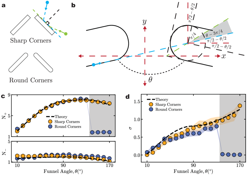
Extended Data Fig. 1: Comparison between sharp and round cornered funnel geometries. a, Schematic showing sharp and round cornered funnel geometries. b, Schematic showing the region near the funnel tip for round-cornered funnel in the obtuse $\theta$ regime. Particles arriving at the funnel tip along the funnel wall (blue dashed line) get rectified (go in the $+y$ direction after collision with the adjacent funnel wall) only if the blue line is above the green line, which is when the gray shaded region is not present (when $\theta<3\pi/4$). This leads to a sharp drop in $N_{+}$ and $\sigma$ for $\theta>3\pi/4$. c, $N_{+}$ and $N_{-}$ plotted for sharp and round cornered funnel geometries. c, $\sigma$ plotted for sharp and round cornered funnel geometries. $\theta>3\pi/4$ shaded in gray in c and d. All shaded regions denote measurement standard deviations.

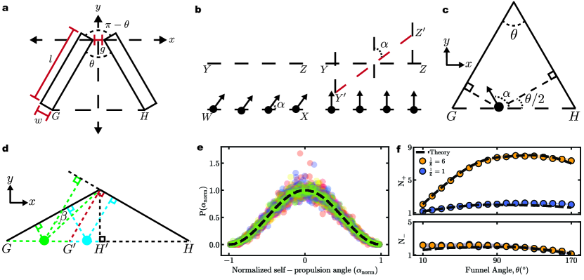
Extended Data Fig. 2: Mechanical model of bacterial rectification. a, Schematic showing a funnel rectifier with labeled geometrical parameters. b, Schematic showing the reasoning used in the derivation of the distribution of self-propulsion angles $\alpha$ of particles reaching a line. Schematic showing the inside of funnel rectifier for acute $\theta$ (c), and obtuse $\theta$ (d), with solid black lines indicating the funnel walls. e, Plot of probability distribution of normalized self-propulsion angles ($\alpha_{norm}$) reaching the funnel gate $GH$. The dashed black line shows predictions from eqn. 8. Symbols of different colors correspond to different $\theta$. f, $N_{+}$ and $N_{-}$ plotted with $\theta$ for two different funnel geometries. The dashed black line shows predictions from eqns. 16 and 17. Shaded regions denote measurement standard deviations.

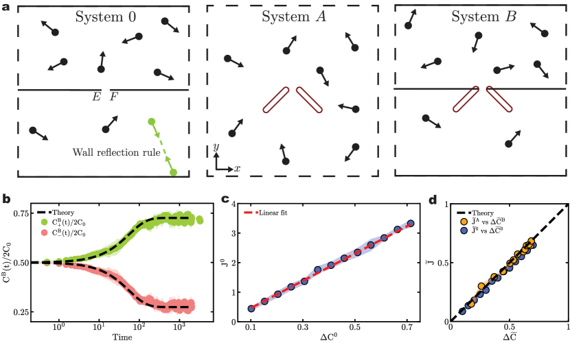
Extended Data Fig. 3: Generalized mass transfer relation for bacterial rectification. a, Schematic showing three different Systems: $0$, $A$, and $B$. Funnel rectifiers are shown in red. Solid black lines represent boundary walls and dashed black lines denote periodic boundary conditions. Flux is measured in all three systems at the imaginary line $EF$ at the gap connecting the $+y$ and $-y$ sides of the chamber. b, Time evolution of concentration in $+y$ and $-y$ regions in System $B$ starting from an initial concentration of $C_{0}$ in both regions for $\theta=20\degree$. Dashed black lines show predictions from eqn. 31. c, Plot showing $J$ and $\Delta C$ measured in System $0$. The red dashed line shows a linear fit used to extract the mass transfer coefficient $k$. d, Normalized flux per particle $\widetilde{J}$ plotted with normalized concentration difference per particle $\Delta\widetilde{C}$ for $\widetilde{J}$ measured in System $A$ and $\Delta\widetilde{C}$ measured in System $B$, and also for both quantities measured in System $0$. The black dashed line shows predictions from Eq. (34). All shaded regions denote measurement standard deviations.

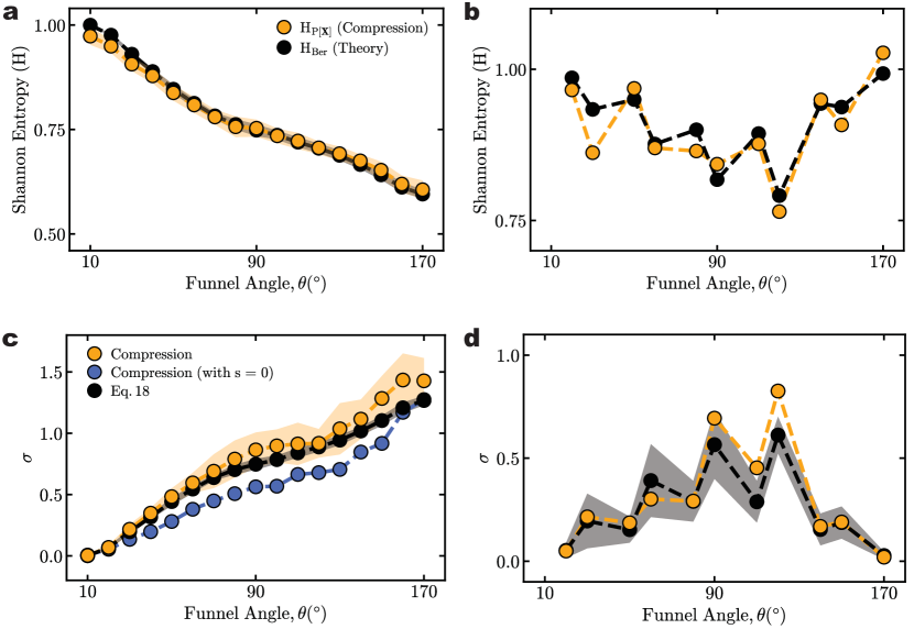
Extended Data Fig. 4: Shannon entropy and time-irreversibility measured using compression-based estimators. Shannon entropy $H$ of time-forward sequence of states $P[\textbf{X}]$ plotted with funnel angle $\theta$ for minimal simulations (a), and experiments (b). Time-irreversibility, $\sigma$, plotted with $\theta$ for minimal simulations (c), and experiments (d). All shaded regions denote measurement standard deviations.

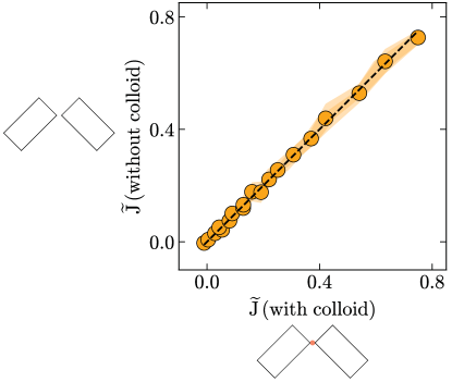
Extended Data Fig. 5: Weak-coupling assumption in the ideal work measurement scenario. Plot showing normalized flux per particle, $\widetilde{J}$, for the system shown in Fig. 4a with and without a harmonically trapped colloid at the tip of the funnel rectifier. Shaded regions denote measurement standard deviations.

References

- Schrodinger [2012] E. Schrodinger, What is Life? (Cambridge Univ. Press, 2012).
- Jarzynski [2011] C. Jarzynski, Annu. Rev. Condens. Matter Phys. 2, 329 (2011).
- Seifert [2012] U. Seifert, Reports on progress in physics 75, 126001 (2012).
- Peliti and Pigolotti [2021] L. Peliti and S. Pigolotti, Stochastic Thermodynamics: An Introduction (Princeton University Press, 2021).
- De Groot and Mazur [2013] S. R. De Groot and P. Mazur, Non-equilibrium thermodynamics (Courier Corporation, 2013).
- Martínez et al. [2017] I. A. Martínez, É. Roldán, L. Dinis, and R. A. Rica, Soft matter 13, 22 (2017).
- Fodor and Cates [2021] É. Fodor and M. E. Cates, Europhysics Letters 134, 10003 (2021).
- Krishnamurthy et al. [2016] S. Krishnamurthy, S. Ghosh, D. Chatterji, R. Ganapathy, and A. Sood, Nature Physics 12, 1134 (2016).
- Pietzonka et al. [2019] P. Pietzonka, É. Fodor, C. Lohrmann, M. E. Cates, and U. Seifert, Physical Review X 9, 041032 (2019).
- Angelani et al. [2009] L. Angelani, R. Di Leonardo, and G. Ruocco, Physical review letters 102, 048104 (2009).
- Di Leonardo et al. [2010] R. Di Leonardo, L. Angelani, D. Dell’Arciprete, G. Ruocco, V. Iebba, S. Schippa, M. P. Conte, F. Mecarini, F. De Angelis, and E. Di Fabrizio, Proceedings of the National Academy of Sciences 107, 9541 (2010).
- Kaiser et al. [2014] A. Kaiser, A. Peshkov, A. Sokolov, B. Ten Hagen, H. Löwen, and I. S. Aranson, Physical review letters 112, 158101 (2014).
- Li and Zhang [2013] H. Li and H. Zhang, Europhysics Letters 102, 50007 (2013).
- Sokolov et al. [2010] A. Sokolov, M. M. Apodaca, B. A. Grzybowski, and I. S. Aranson, Proceedings of the National Academy of Sciences 107, 969 (2010).
- Angelani and Di Leonardo [2010] L. Angelani and R. Di Leonardo, New Journal of physics 12, 113017 (2010).
- Reichhardt and Reichhardt [2017] C. O. Reichhardt and C. Reichhardt, Annual Review of Condensed Matter Physics 8, 51 (2017).
- Cates [2012] M. E. Cates, Reports on Progress in Physics 75, 042601 (2012).
- Galajda et al. [2007] P. Galajda, J. Keymer, P. Chaikin, and R. Austin, Journal of bacteriology 189, 8704 (2007).
- Drocco et al. [2012] J. A. Drocco, C. O. Reichhardt, and C. Reichhardt, Physical Review E 85, 056102 (2012).
- Martinez et al. [2020] R. Martinez, F. Alarcon, J. L. Aragones, and C. Valeriani, Soft matter 16, 4739 (2020).
- Guidobaldi et al. [2014] A. Guidobaldi, Y. Jeyaram, I. Berdakin, V. V. Moshchalkov, C. A. Condat, V. I. Marconi, L. Giojalas, and A. V. Silhanek, Physical Review E 89, 032720 (2014).
- Wan et al. [2008] M. Wan, C. O. Reichhardt, Z. Nussinov, and C. Reichhardt, Physical review letters 101, 018102 (2008).
- Reichhardt et al. [2011] C. O. Reichhardt, J. Drocco, T. Mai, M. Wan, and C. Reichhardt, in Optical Trapping and Optical Micromanipulation VIII, Vol. 8097 (SPIE, 2011) pp. 55–67.
- Tailleur and Cates [2009] J. Tailleur and M. Cates, Europhysics Letters 86, 60002 (2009).
- Ro et al. [2022] S. Ro, B. Guo, A. Shih, T. V. Phan, R. H. Austin, D. Levine, P. M. Chaikin, and S. Martiniani, Physical Review Letters 129, 220601 (2022).
- Galajda et al. [2008] P. Galajda, J. Keymer, J. Dalland, S. Park, S. Kou, and R. Austin, Journal of Modern Optics 55, 3413 (2008).
- Lambert et al. [2010] G. Lambert, D. Liao, and R. H. Austin, Physical review letters 104, 168102 (2010).
- Kantsler et al. [2013] V. Kantsler, J. Dunkel, M. Polin, and R. E. Goldstein, Proceedings of the National Academy of Sciences 110, 1187 (2013).
- Sparacino et al. [2020] J. Sparacino, G. L. Miño, A. J. Banchio, and V. I. Marconi, Journal of Physics D: Applied Physics 53, 505403 (2020).
- Nam et al. [2013] S.-W. Nam, C. Qian, S. H. Kim, D. van Noort, K.-H. Chiam, and S. Park, Scientific Reports 3, 3247 (2013).
- Berg [2004] H. C. Berg, E. coli in Motion (Springer, 2004).
- Hyon et al. [2012] Y. Hyon, T. R. Powers, R. Stocker, H. C. Fu, et al., Journal of Fluid Mechanics 705, 58 (2012).
- Kamdar et al. [2022] S. Kamdar, S. Shin, P. Leishangthem, L. F. Francis, X. Xu, and X. Cheng, Nature 603, 819 (2022).
- O’Byrne et al. [2022] J. O’Byrne, Y. Kafri, J. Tailleur, and F. van Wijland, Nature Reviews Physics 4, 167 (2022).
- Berke et al. [2008] A. P. Berke, L. Turner, H. C. Berg, and E. Lauga, Physical Review Letters 101, 038102 (2008).
- Li and Tang [2009] G. Li and J. X. Tang, Physical review letters 103, 078101 (2009).
- Bianchi et al. [2017] S. Bianchi, F. Saglimbeni, and R. Di Leonardo, Physical Review X 7, 011010 (2017).
- Drescher et al. [2011] K. Drescher, J. Dunkel, L. H. Cisneros, S. Ganguly, and R. E. Goldstein, Proceedings of the National Academy of Sciences 108, 10940 (2011).
- Parrondo et al. [2009] J. M. Parrondo, C. Van den Broeck, and R. Kawai, New Journal of Physics 11, 073008 (2009).
- Roldán [2014] É. Roldán, Irreversibility and dissipation in microscopic systems (Springer, 2014).
- Roldán and Parrondo [2010] É. Roldán and J. M. Parrondo, Physical review letters 105, 150607 (2010).
- Roldán and Parrondo [2012] É. Roldán and J. M. Parrondo, Physical Review E 85, 031129 (2012).
- Gomez-Marin et al. [2008] A. Gomez-Marin, J. Parrondo, and C. Van den Broeck, Europhysics Letters 82, 50002 (2008).
- Kawai et al. [2007] R. Kawai, J. M. Parrondo, and C. Van den Broeck, Physical review letters 98, 080602 (2007).
- Roldán et al. [2021] É. Roldán, J. Barral, P. Martin, J. M. Parrondo, and F. Jülicher, New Journal of Physics 23, 083013 (2021).
- Tan et al. [2021] T. H. Tan, G. A. Watson, Y.-C. Chao, J. Li, T. R. Gingrich, J. M. Horowitz, and N. Fakhri, arXiv preprint arXiv:2107.05701 (2021).
- Jerez et al. [2021] M. J. Y. Jerez, M. A. Bonachita, and M. N. P. Confesor, Physical Review E 104, 044609 (2021).
- Zia and Schmittmann [2007] R. K. Zia and B. Schmittmann, Journal of Statistical Mechanics: Theory and Experiment 2007, P07012 (2007).
- Cussler [2009] E. L. Cussler, Diffusion: mass transfer in fluid systems (Cambridge university press, 2009).