Scaling description of frictionless dense suspensions under inhomogeneous flow

Abstract

Predicting the rheology of dense suspensions under inhomogeneous flow is crucial in many industrial and geophysical applications, yet the conventional ‘$\mu(J)$’ framework is limited to homogeneous conditions in which the shear rate and solids fraction are spatially invariant. To address this shortcoming, we use particle-based simulations of frictionless dense suspensions to derive new constitutive laws that unify the rheological response under both homogeneous and inhomogeneous conditions. By defining a new dimensionless number associated with particle velocity fluctuations and combining it with the viscous number, the macroscopic friction and the solids fraction, we obtain scaling relations that collapse data from homogeneous and inhomogeneous simulations. The relations allow prediction of the steady state velocity, stress and volume fraction fields using only knowledge of the applied driving force.

Introduction.

Dense suspensions are an important class of soft matter system comprising Brownian or non-Brownian particles mixed roughly equally by volume with viscous fluid Ness et al. (2022). Their rheology attracts sustained interest from physicists due to the manifold complex phenomena that arise with apparently simple constituents Stickel and Powell (2005); Jamali et al. (2020). These include non-equilibrium absorbing state transitions Corté et al. (2008), shear thickening Barnes (1989), thinning de Kruif et al. (1985), and yield stress behaviour Richards et al. (2020). As well as being of fundamental interest, characterising this complexity is key to the extensive use of dense suspensions in various formulation and processing industries.

A useful model with which to build rheological understanding is the non-Brownian suspension Guazzelli and Pouliquen (2018), an especially appealing system when one considers the case of inertialess hard spheres. By analogy to dry granular systems Jop et al. (2006), a recent study successfully obtained constitutive laws for this system Boyer et al. (2011), confirming their rate-independence and finding one-to-one relations between the volume fraction $\phi$ and each of two dimensionless rheological quantities, the viscous number $J=\eta\dot{\gamma}/P$ and the macroscopic friction coefficient $\mu=\sigma_{xy}/P$. Here $\eta$ is the suspending liquid viscosity, $\dot{\gamma}$ is the shear rate, $P$ is a measure of the particle contribution to the normal stress, and $\sigma_{xy}$ is the shear stress. This important result, the so-called $\mu(J)$-rheology, forms the basis of subsequent models that introduce rate-dependence through additional stress scales Wyart and Cates (2014); Guy et al. (2018).

The applicability of $\mu(J)$ becomes limited when considering inhomogeneous flows in which $\dot{\gamma}$ varies spatially Hampton et al. (1997); Oh et al. (2015); Gillissen and Ness (2020). In particular, the lower limit of $\mu$ (which we denote $\mu_{J}$) is non-zero in all homogeneously flowing systems irrespective of the particle-particle friction coefficient $\mu_{p}$ Da Cruz et al. (2005); Chialvo et al. (2012); Cheal and Ness (2018) but can by construction vanish when mechanical balance dictates sign changes in $\sigma_{xy}$ such as along pipe centrelines. In such scenarios regions that would otherwise be jammed (i.e. with $\mu<\mu_{J}$ and $J=0$) can have non-zero $\dot{\gamma}$ thanks to facilitation by nearby flowing regions Saitoh and Tighe (2019); Pouliquen and Forterre (2009). This non-local effect has been extensively studied in amorphous solids Goyon et al. (2008) and dry granular systems Kamrin and Koval (2012), often by formulating a fluidity field with diffusive behaviour characterised by an inhomogeneous Helmholtz equation. Microscopically it is conceptualized that the fluidity originates from an activated process that diffuses through the system in a cooperative way controlled by an inherent length scale Goyon et al. (2008); Bocquet et al. (2009); Kamrin and Koval (2012); Saitoh and Tighe (2019); Bouzid et al. (2013). Recent works in dry granular matter Zhang and Kamrin (2017); Kim and Kamrin (2020); Gaume et al. (2020) interpret the fluidity in terms of particle velocity fluctuations $\delta u$ and density $\rho$, defining a fourth dimensionless quantity $\Theta=\rho\delta u^{2}/P$ and seeking constitutive relations linking it to $\phi$, $\mu$ and $I$ Jop et al. (2006) (the dry counterpart to $J$). This successfully collapses data from homogeneous and inhomogeneous simulations onto a master curve, but is limited in that the $\Theta$ fields required to make predictions thereafter must be obtained by simulation. Naturally such findings raise the question of whether similar constitutive equations exist to unify homogeneous and inhomogeneous dense suspension rheology.

Here we use particle-based simulation Cundall and Strack (1979) to model dense suspensions under homogeneous and inhomogeneous conditions, achieving the latter through an imposed Kolmogorov flow following the approach of Saitoh and Tighe (2019). We seek to unify the rheology under both sets of conditions by first defining a dimensionless suspension temperature based on particle velocity fluctuations, as $\Theta=\eta\delta u/aP$, analogous to the granular temperature Kim and Kamrin (2020), and then obtaining relations among the four dimensionless numbers $\phi$, $J$, $\mu$ and $\Theta$. Although the $\mu(J)$ framework was devised based on frictional millimetric grains, recent experiments demonstrate it is nonetheless applicable to frictionless ones Etcheverry et al. (2023), and we focus here on the latter. Doing so we find scalings that can collapse homogeneous and inhomogeneous rheology data onto a set of master curves that can then be used to predict the rheology of other flow types.

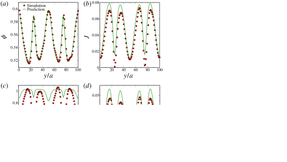
Figure 1: Inhomogeneous flow of a frictionless dense suspension. Shown are (a) a typical configuration of the system for $\bar{\phi}=0.60$, with the red region highlighting a coarse-graining box; and the steady-state profiles in $y$ of (b) the $x$-components of the externally applied liquid velocity field $u_{x}^{\infty}$ (green line) and the coarse-grained velocity field of the particles ${u}_{x}$ (red points). Velocity is presented here in units of $\kappa$; (c) the expected shear rate for a Newtonian fluid $\dot{\gamma}^{\infty}=\partial u_{x}^{\infty}/\partial y$ (green line) and the measured shear rate $\dot{\gamma}$ (red points), both in units of $\kappa/a$; (d) the velocity fluctuations $\delta u$ in units of $\kappa$; (e) the local volume fraction $\phi$, noting that the higher values at low $\dot{\gamma}$ demonstrate particle migration has taken place; (f) the pressure $P$ expressed in units of $\eta\kappa/a$; (g) the shear stress $\sigma_{xy}$ computed from the particle interactions (red points) and by integrating over the left hand side of Eq. 4 (green points), in the same units as $P$.

Simulations details.

We simulate a mixture of frictionless, non-Brownian spheres of radius $a$ and $1.4a$ mixed in equal number in a periodic box of dimensions $L_{x}$, $L_{y}$, $L_{z}$, using LAMMPS Plimpton (1995); Ness (2023) (see Fig. 1(a)). Particles are suspended in a density ($\rho$) matched viscous liquid, and we impose pairwise contact and hydrodynamic forces as described by Ref.Cheal and Ness (2018). Briefly, the hydrodynamic lubrication force for particles of radius $a_{i}$ and $a_{j}$, with center-to-center vector $\bm{r}_{i,j}$, is given by $\bm{F}^{h}_{i,j}\sim(1/h)\mathbf{u}_{i,j}$, where $\mathbf{u}_{i,j}$ is the relative velocity of the particles and $h=(a_{i}+a_{j})-|\bm{r}_{i,j}|$. $F^{h}_{i,j}$ is not computed for $h>0.05a$, and it saturates to $\sim(1/h^{c})\mathbf{u}_{i,j}$ for $h\leq h^{c}$ (with $h^{c}=0.001a$), allowing particles to come into contact. Contact forces arise only when $|\bm{r}_{i,j}|<(a_{i}+a_{j})$ and are given by $\bm{F}^{c}_{{i,j}}=k\left[(a_{i}+a_{j})-|\bm{r}_{i,j}|\right]\mathbf{n}_{ij}$, where $k$ is a spring constant and $\mathbf{n}_{i,j}=\bm{r}_{i,j}/|\bm{r}_{i,j}|$. Particles additionally experience dissipative drag due to motion relative to the fluid, given by $\bm{F}^{d}_{i}=6\pi\eta a\left(\bm{u}_{i}-\bm{u}^{\infty}(y_{i})\right)$, with $\bm{u}_{i}$ the velocity of particle $i$ and $\bm{u}^{\infty}(y_{i})$ the liquid streaming velocity at the position of particle $i$.

Flow is generated by specifying $\bm{u}^{\infty}$ to induce particle motion through drag. We obtain homogeneous rheology data for fixed-volume systems of $\phi=0.48$ to $0.65$ by generating simple shear via $\bm{u}^{\infty}(y)=\dot{\gamma}y\bm{\delta}_{x}$, with $y$ the direction of the velocity gradient and $\bm{\delta}_{x}$ the unit vector along $x$. We chose our parameters such that $\rho\dot{\gamma}a^{2}/\eta\ll 1$ and $\dot{\gamma}\sqrt{\rho a^{3}/k}\ll 1$, recovering rate-independence Boyer et al. (2011). To obtain inhomogeneous flow we specify a spatially dependent liquid velocity as $\bm{u}^{\infty}(y)=\kappa\sin\left(2\pi y/L_{y}\right)\bm{\delta}_{x}$ (see Fig. 1(b), and the gradient $\dot{\gamma}^{\infty}$ in Fig. 1(c)), and later test the model with $\bm{u}^{\infty}(y)=\kappa\sin^{3}(2\pi y/L_{y})\bm{\delta}_{x}$. We run simulations with $L_{y}=50a$, $100a$ and $200a$ (with $L_{x},L_{z}=20a$) and systems containing $\mathcal{O}(10^{4})$ particles (we verified that larger systems produce equivalent rheology results). We simulated systems with mean volume fraction $\bar{\phi}=0.5$ to $0.63$ (achieved by varying the particle number), and $\kappa$ is a constant with dimensions of velocity, chosen so that the measured $\rho\dot{\gamma}a^{2}/\eta$ remains $<0.01$ throughout and particle inertia is negligible. The stress (a tensor) is computed on a per-particle basis as $\mathbb{\Sigma}_{i}=\sum_{j}(\bm{F}_{i,j}^{*}\otimes\bm{r}_{i,j})$, counting both contact and hydrodynamic forces.

We aim to compare the spatially-variant values of $J$, $\mu$, $\phi$ and $\Theta$ obtained via inhomogeneous flow with the spatially-invariant ones obtained via homogeneous flow (the latter follow closely our previous results Cheal and Ness (2018)). Doing so requires computing the variation in $y$ of the stress and velocity fields under inhomogeneous flow, which we do by binning particle data in blocks of width $a$ and volume $V_{b}=L_{x}aL_{z}$, with the per-block value of a quantity being simply the mean of the per-particle quantities of the particles with centers lying therein. We compute the velocity fluctuation (necessary for calculating the $\Theta$ field) of each particle as $\delta u_{i}=|u_{i,x}-{u}^{\dagger}_{i,x}|$ where $u_{i,x}$ is the $x$-component of $\bm{u}_{i}$ and ${u}^{\dagger}_{i,x}$ is the average $x$ velocity of all particles with centers lying in a narrow window $\pm\epsilon$ (taking $\epsilon=\mathcal{O}(0.1a)$) of $y$, and we then bin $\delta u_{i}$ per block. As all three components of the velocity fluctuations are statistically equivalent we have used only the $x$ values to compute $\Theta$. In what follows we report steady state data only foo , averaging across 6 realizations and at least 500 configurations per realization.

Figure 2: Relations between the dimensionless control parameters. Shown in the top row are the relations between the dimensionless viscous number $J$ and (a) the volume fraction $\phi$ for a range of homogeneous $\phi$ (black data) and inhomogeneous $\bar{\phi}$; (b) the effective friction coefficient $\mu$ and; (c) the suspension temperature $\Theta$. In the bottom row are the collapses using the scaling Eqns. 1 (d), 2 (e) and 3 (f), for different $\bar{\phi}$ and $L$. In (d) we show data for $L/a=50$ to highlight its deviation from the scaling relation. Black triangles represent homogeneous data (simple shear) and all other points are for inhomogeneous flow at different $\bar{\phi}$.

Results.

Shown in Fig. 1(b)-(g) are, respectively, steady-state profiles in $y$ of the coarse-grained velocity (in $x$) $u_{x}$, shear rate $\dot{\gamma}=\partial u_{x}/\partial y$, velocity fluctuations $\delta u$, volume fraction $\phi$, pressure $P$ ($=(1/3)\text{Tr}(\mathbb{\Sigma}$)), and shear stress $\sigma_{xy}$, for $\bar{\phi}=0.60$, with each plotted point representing a block. Although at initialisation the particle density is homogeneous (i.e. $\phi\neq\phi(y)$), in the steady state $\phi$ exhibits spatial variation set up by particle migration to balance the normal stress Hampton et al. (1997); Oh et al. (2015); Morris and Boulay (1999). The velocity profile follows a similar trend to the applied force, as expected, but is flattened at the regions of largest $\phi$ leading to significant deviations between $\dot{\gamma}$ and $\dot{\gamma}^{\infty}$. The pressure becomes spatially uniform, and the shear stress follows the shear rate in sign. Since $P$ is spatially invariant in the steady state, one can deduce that the variation of the quantities $\eta\dot{\gamma}/P$, $\sigma_{xy}/P$ and $\eta\delta u/aP$ follow $\dot{\gamma}$, $\sigma_{xy}$ and $\delta u$ respectively.

We analyse inhomogeneous data by computing the dimensionless control parameters in each block, defining the scalar shear rate and stress components on the basis of invariants of the respective tensor quantities so that $J,\mu>0$. This is done for a range of $\bar{\phi}$, with parametric plots of $J(y)$, $\phi(y)$, $\mu(y)$ and $\Theta(y)$ shown in Figs. 2(a)-(c). Each plotted point represents a $y$-coordinate, and colors represent different $\bar{\phi}$. Shown also (in black) are homogeneous data. Reading across the data points of a single color from right-to-left represents moves from regions of high-to-low $\dot{\gamma}$ in the inhomogeneous domain.

The homogeneous $\phi(J)$ and $\mu(J)$ relations follow qualitatively the result of Boyer et al. (2011), though our frictionless particles render $\phi_{J}$ and $\mu_{J}$ dissimilar. $\Theta(J)$ follows a power-law relation, as in dry granular matter Kim and Kamrin (2020) though with a different exponent. In general large-$J$ inhomogeneous data approximately match homogeneous data, though they deviate with decreasing $J$ demonstrating the shortcomings of the existing constitutive laws.

With the help of scaling theory, we next attempt to find constitutive laws that simultaneously describe the rheology under homogeneous and inhomogeneous flow. We focus first on how the inverse viscosity $J/\mu=\eta\dot{\gamma}/\sigma_{xy}$ vanishes as $\phi$ approaches the jamming point $\phi_{J}$. This trend is followed by all the homogeneous and inhomogeneous simulations, leading to our first scaling relation

$$J/\mu=\alpha\left(\phi_{J}-\phi\right)^{2}\text{,}$$ (1)

plotted in Fig. 2(d) with $\alpha=4.1$ and $\phi_{J}=0.6555$.

The next scaling relation is motivated by Kim and Kamrin (2020). In homogeneous flow, within the range of our data we find $\mu^{2.5}\sim J$ (Fig. 2(b)) and $\Theta^{1.44}\sim J$ (Fig. 2(c)). Since for the range of $\bar{\phi}$ explored here inhomogeneous data follow homogeneous laws at large $J$, we expect a scaling of the form $\mu^{2.5}\Theta^{1.44}\sim F_{1}(J)$. Indeed this results in a good collapse as shown in Fig. 2(e), in which data are described by the relation

$$\Theta^{1.44}\mu^{2.5}=\begin{cases}\beta J^{2}&\text{if $J>10^{-3}$};\\ \vartheta J^{1.33}&\text{if $J\leq 10^{-3}$};\\ \end{cases}$$ (2)

with $\beta=3$ and $\vartheta=0.06$.

The final scaling relation is motivated by the relation between granular fluidity and $\phi$ reported for dry granular matter. Zhang and Kamrin (2017) write a non-dimensional granular fluidity $\tilde{g}=gd/\delta u$, where $g=\dot{\gamma}/\mu$, and $d$ is the spatial dimension. We define an equivalent quantity in terms of the previously discussed dimensionless numbers, namely $J/\mu\Theta$, though we find a better collapse is achieved through a change to the exponents as

$$\frac{J}{\Theta^{0.8}\mu^{1.2}}=F_{2}(\phi)\text{,}$$ (3)

with $F_{2}(\phi)=\epsilon\left[(\phi-\phi_{m})+\sqrt{(\phi-\phi_{m})^{2}+\zeta}\right]+\lambda\phi$ (see Fig. 2(f)) and $\epsilon=-10.98$, $\phi_{m}=0.618$, $\zeta=0.0004$ and $\lambda=1.533$. We thus have three scaling relations, Eqs. 1, 2 and 3, that relate $\phi$, $J$, $\mu$ and $\Theta$. The collapse appears poorer for $\bar{\phi}=0.5$ (Fig. 2(f)) and $L/a=50$ (Fig. 2(d)), indicating limits to the range of applicability. An issue in the former case may be that our simplified hydrodynamics, accounting only for lubrication, becomes nonphysical at lower $\phi$ and that a more highly resolved fluid field is required.

Given a profile of one of the dimensionless numbers, one could therefore fully characterise the rheology of the system. In our simulations, however, the only known input is the externally applied force, which we recall is defined through $\bm{u}^{\infty}$. To use the scaling relations we need to establish another relation that can provide us one of these dimensionless numbers from the knowledge of the applied force profile. Considering the inertia-free momentum balance $\nabla\cdot\mathbb{\Sigma}=-\bm{f}$ per unit volume, we can write the following equation for the $k^{th}$ block of the simulation cell (which we verified in Fig. 1(g)):

$$N_{k}6\pi\eta a\left[Au_{x,k}^{\infty}-u_{x,k}\right]=-\left(\frac{\partial\sigma_{xy,k}}{\partial y}\right)V_{b}\text{.}$$ (4)

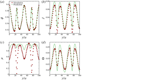
Figure 3: Predictions of the scaling relations against simulation data not used for obtaining the scaling exponents, with $\bm{u}^{\infty}(y)=\kappa\sin^{3}(2\pi y/L_{y})\bm{\delta}_{x}$. Shown are (a) the volume fraction $\phi$; (b) the viscous number $J$; (c) the effective friction coefficient $\mu$; and (d) the suspension temperature $\Theta$, with predictions given by solid lines and simulation data in points, for $\bar{\phi}=0.55$ (red) and $0.57$ (green).

Here $N_{k}$, $u_{x,k}^{\infty}$, $u_{x,k}$ and $\sigma_{xy,k}$ are the particle number in the block, the liquid streaming velocity at the centre of the block, and the particle velocity and stress averaged over the block, which has volume $V_{b}$. $A$ is an order unity quantity necessary to account for small variations in $u_{x,k}^{\infty}$ across the block. The first term of Eq. 4 represents the net applied force and the second represents the net viscous force exerted by the fluid due to drag. The resultant of these is balanced by the net stress gradient inside the block. Using the definition of our dimensionless numbers, Eq. 4 can be rewritten for the streaming velocity at $y$ as

$$u_{x}^{\prime\infty}(y)=\left[\int_{0}^{y}\frac{1}{a}J^{*}(y^{\prime})dy^{\prime}-\frac{2a}{9\phi(y)}\left(\frac{\partial\mu^{*}(y)}{\partial y}\right)\right]\text{,}$$ (5)

with $u_{x}^{\prime\infty}(y)=u_{x}^{\infty}(y)\eta A/aP$ and asterisks representing multiplication by $\mathrm{sgn}(\dot{\gamma}^{\infty}(y))$, noting that $P$ is uniform at steady state and using $\phi(y)=(4/3)\pi a^{3}N(y)/V_{b}$, acknowledging our earlier comment about phase separation foo . Equation 5 thus relates the externally applied liquid flow field to the profiles of $J$, $\mu$ and $\phi$.

For a known $\bm{u}^{\infty}$ we solve Eqs. 1, 2, 3 and 5 numerically in the following way. We first guess a $\phi\left(y\right)$ profile by assuming accumulation at points where the spatial derivative of the imposed force vanishes, starting with a simple form as $\phi(y)=\sum_{j=1}^{n_{p}}a_{j}/[(y-y^{0}_{j})^{2}+b^{2}_{j}]+\phi_{0}$, with mass conserved through $\bar{\phi}=\frac{1}{L_{y}}\int_{0}^{L_{y}}\phi\left(y\right)dy$. Here $y^{0}_{j}$ are the coordinates of the point where the first derivative of the applied force vanishes, $n_{p}$ is the number of such points and $b_{j}$ is the width of the Lorentzian function peaked at $y^{0}_{j}$. We then compute directly $J$, $\mu$ and $\Theta$ using Eqs. 1, 2 and 3, before attempting to balance Eq. 5. The imbalance of Eq. 5 reflects the accuracy of our guess. We refine $\phi(y)$ by tuning $\phi_{0}$, $a_{j}$ and $b_{j}$ until Eq. 5 is satisfied (up to some tolerance). Shown in Fig. 3 are predicted results compared against ‘unseen’ simulation data (i.e. data not used to obtain the scaling exponents) with $\bar{\phi}=0.55$, $0.57$ and $\bm{u}^{\infty}(y)=\kappa\sin^{3}(2\pi y/L_{y})\bm{\delta}_{x}$, demonstrating the degree of success of the scaling relations for predicting $y$-profiles of $\phi$, $J$, $\mu$ and $\Theta$. Considering the highly non-linear nature of the scaling relations, the quality of the predictions is reasonably good.

Conclusions.

Using particle-based simulation we seek universality amongst flows of dense, frictionless suspensions. Along with canonical suspension rheology control parameters $\phi$, $J$ and $\mu$, we introduce a fourth quantity $\Theta$ characterising velocity fluctuations, inspired by recent studies in dry granular physics Kim and Kamrin (2020). We find a trio of scaling relations among these quantities that collapse data for homogeneous and inhomogeneous flow. Utilising a momentum balance we show that from knowledge of the externally applied force, one can use the relations to predict the features of a general inhomogeneous flow. Our work raises manifold avenues for future work. In particular, the microscopic origin of the exponents is not understood, nor is their generalisation to the broader class of suspensions that includes polydisperse particles (for which colloidal forces may become relevant Li et al. (2023)), non-spheres and other complexities. Meanwhile the question of a diverging lengthscale —apparently a staple of non-local rheology in dry granular matter Bouzid et al. (2013); Kamrin and Koval (2012); Tang et al. (2018)— remains open. Computing a granular fluidity field from our data, we find, similar to Saitoh and Tighe (2019), no divergence in the characteristic lengthscale, which remains $\mathcal{O}(a)$ everywhere. This raises an important open question regarding what are the minimal conditions required for a diverging lengthscale in inhomogeneous particulate flows.

B.P.B. acknowledges support from the Leverhulme Trust under Research Project Grant RPG-2022-095; C.N. acknowledges support from the Royal Academy of Engineering under the Research Fellowship scheme. We thank Ken Kamrin, Martin Trulsson, Mehdi Bouzid, Romain Mari and Jeff Morris for useful discussions.

References

- Ness et al. (2022) C. Ness, R. Seto, and R. Mari, Annual Review of Condensed Matter Physics 13, 97 (2022).
- Stickel and Powell (2005) J. J. Stickel and R. L. Powell, Annual Review of Fluid Mechanics 37, 129 (2005).
- Jamali et al. (2020) S. Jamali, E. Del Gado, and J. F. Morris, Journal of Rheology 64, 1501 (2020).
- Corté et al. (2008) L. Corté, P. M. Chaikin, J. P. Gollub, and D. J. Pine, Nature Physics 4, 420 (2008).
- Barnes (1989) H. A. Barnes, Journal of Rheology 33, 329 (1989).
- de Kruif et al. (1985) C. G. de Kruif, E. M. F. van Iersel, A. Vrij, and W. B. Russel, Journal of Chemical Physics 83, 4717 (1985).
- Richards et al. (2020) J. Richards, B. Guy, E. Blanco, M. Hermes, G. Poy, and W. Poon, Journal of Rheology 64, 405 (2020).
- Guazzelli and Pouliquen (2018) É. Guazzelli and O. Pouliquen, Journal of Fluid Mechanics 852, P1 (2018).
- Jop et al. (2006) P. Jop, Y. Forterre, and O. Pouliquen, Nature 441, 727 (2006).
- Boyer et al. (2011) F. Boyer, E. Guazzelli, and O. Pouliquen, Physical Review Letters 107, 188301 (2011).
- Wyart and Cates (2014) M. Wyart and M. E. Cates, Physical Review Letters 112, 098302 (2014).
- Guy et al. (2018) B. Guy, J. Richards, D. Hodgson, E. Blanco, and W. Poon, Physical review letters 121, 128001 (2018).
- Hampton et al. (1997) R. E. Hampton, A. A. Mammoli, A. L. Graham, N. Tetlow, and S. A. Altobelli, Journal of Rheology 41, 621 (1997).
- Oh et al. (2015) S. Oh, Y.-q. Song, D. I. Garagash, B. Lecampion, and J. Desroches, Physical Review Letters 114, 088301 (2015).
- Gillissen and Ness (2020) J. J. J. Gillissen and C. Ness, Physical Review Letters 125, 184503 (2020).
- Da Cruz et al. (2005) F. Da Cruz, S. Emam, M. Prochnow, J.-N. Roux, and F. Chevoir, Physical Review E 72, 021309 (2005).
- Chialvo et al. (2012) S. Chialvo, J. Sun, and S. Sundaresan, Physical Review E 85, 021305 (2012).
- Cheal and Ness (2018) O. Cheal and C. Ness, Journal of Rheology 62, 501 (2018).
- Saitoh and Tighe (2019) K. Saitoh and B. P. Tighe, Physical Review Letters 122, 188001 (2019).
- Pouliquen and Forterre (2009) O. Pouliquen and Y. Forterre, Philosophical Transactions of the Royal Society A: Mathematical, Physical and Engineering Sciences 367, 5091 (2009).
- Goyon et al. (2008) J. Goyon, A. Colin, G. Ovarlez, A. Ajdari, and L. Bocquet, Nature 454, 84 (2008).
- Kamrin and Koval (2012) K. Kamrin and G. Koval, Physical Review Letters 108, 178301 (2012).
- Bocquet et al. (2009) L. Bocquet, A. Colin, and A. Ajdari, Physical Review Letters 103, 036001 (2009).
- Bouzid et al. (2013) M. Bouzid, M. Trulsson, P. Claudin, E. Clément, and B. Andreotti, Physical Review Letters 111, 238301 (2013).
- Zhang and Kamrin (2017) Q. Zhang and K. Kamrin, Physical Review Letters 118, 058001 (2017).
- Kim and Kamrin (2020) S. Kim and K. Kamrin, Physical Review Letters 125, 088002 (2020).
- Gaume et al. (2020) J. Gaume, G. Chambon, and M. Naaim, Physical Review Letters 125, 188001 (2020).
- Cundall and Strack (1979) P. A. Cundall and O. D. L. Strack, Géotechnique 29, 47 (1979).
- Etcheverry et al. (2023) B. Etcheverry, Y. Forterre, and B. Metzger, Physical Review X 13, 011024 (2023).
- Plimpton (1995) S. Plimpton, Journal of Computational Physics 117, 1 (1995).
- Ness (2023) C. Ness, Computational Particle Mechanics , 1 (2023).
- (32) There is in fact a very slow phase separation of small and large particles driven by the shear rate gradient, so we keep run times sufficiently short that no significant re- distribution occurs and our data represent uniform mix- tures .
- Morris and Boulay (1999) J. F. Morris and F. Boulay, Journal of rheology 43, 1213 (1999).
- Li et al. (2023) X. Li, J. R. Royer, and C. Ness, arXiv preprint arXiv:2307.13802 (2023).
- Tang et al. (2018) Z. Tang, T. A. Brzinski, M. Shearer, and K. E. Daniels, Soft matter 14, 3040 (2018).