Continuous Sweep: an improved, binary quantifier.

Abstract

Quantification is a supervised machine learning task, focused on estimating the class prevalence of a dataset rather than labeling its individual observations. We introduce Continuous Sweep, a new parametric binary quantifier inspired by the well-performing Median Sweep [1]. Median Sweep is currently one of the best binary quantifiers, but we have changed this quantifier on three points, namely 1) using parametric class distributions instead of empirical distributions, 2) optimizing decision boundaries instead of applying discrete decision rules, and 3) calculating the mean instead of the median. We derive analytic expressions for the bias and variance of Continuous Sweep under general model assumptions. This is one of the first theoretical contributions in the field of quantification learning. Moreover, these derivations enable us to find the optimal decision boundaries. Finally, our simulation study shows that Continuous Sweep outperforms Median Sweep in a wide range of situations.

MSC Classification]68U99

1 Introduction

Accurately estimating prevalences often plays a crucial role in critical real-world problems. In epidemiology, the prevalence of COVID-19 in the population determined how governments responded to the pandemic [2, 3]. In political science, polls and sentiment analysis are used to predict the prevalence of votes in presidential elections [4]. Furthermore, in ecology, the prevalence of coral reef and plankton populations in oceans [5] provide essential information on the state of nature. In each of these examples, the task is to determine the prevalence of a single class within a population. This task is referred to as the quantification task [6].

The quantification task is trivial when the class labels are known or when they can be predicted without error for the entire population. In practice, the class labels are usually known for a small subset of the population only and the prediction of class labels for the rest of the population is never free from error. Such errors are referred to as misclassifications. If misclassifications occur, the prevalence estimate based on known and predicted class labels is often biased. This bias is known as misclassification bias [7]. Fig. 1 shows the size and sign of misclassification bias when we consider a binary classification problem. It shows that the prevalence estimate in a binary classification problem is unbiased if and only if the number of false positives is equal to the number of false negatives. Moreover, it can be shown that the size of misclassification bias does not decrease with increasing population size, as long as the probabilities that misclassifications occur stay the same.

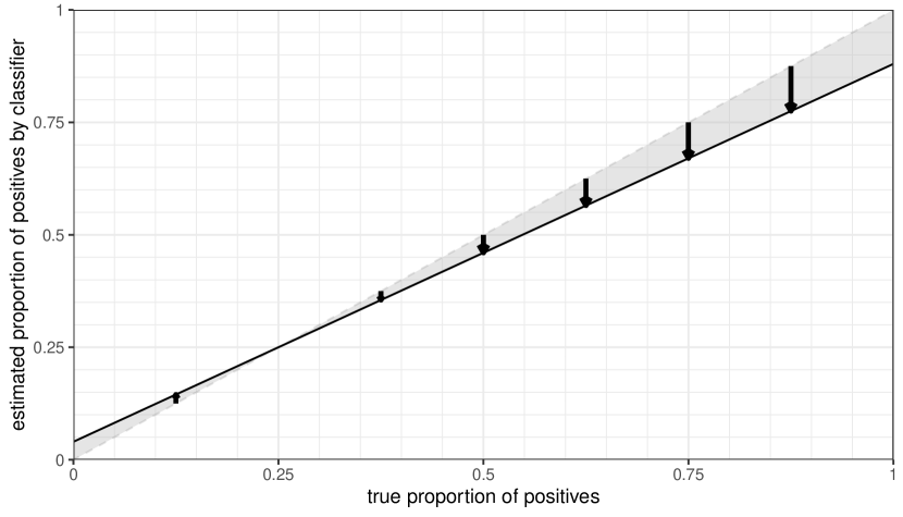
Figure 1: The bias of a classifier on the proportion estimate. Based on a classifier with an accuracy of $88\%$ on the positive labeled observations and an accuracy of $96\%$ on the negative labeled observations. If the prevalence estimate is unbiased, the prevalence value would lay on the dashed, grey line. The black line denotes the expected value of the estimated prevalence by counting the estimated labels of a classifier. The black arrows combined with the grey area denote the severity of the misclassification bias.

The first analysis of misclassification bias appeared in the 1950s when Bross elaborated on the impact of systematic misclassifications of disease diagnoses on chi-square tests [8]. In the decades that followed, many fields discovered the impact of misclassification bias and henceforth a lot of statistical methods to correct for that bias were developed. In the 1990s, Kuha and Skinner provided an overview of the most relevant ones while applying them on mislabeled questions for census data [9].

In the field of machine learning, the quantification task first appeared as a side-product of classification. Supervised classifiers predict the labels of an unlabeled data set trained on a labeled training set. Any classifier is imperfect, so the predicted labels in the unlabeled test set contain misclassifications. Consequently, when counting the predicted labels in that test set, misclassification bias in the prevalence estimate occurs. In 2005, Forman introduced quantification as a standalone machine learning task and named it quantification learning [10]. In quantification learning, we are particularly interested in tasks where the prevalence in the correctly labeled training data is different from the prevalence in the unlabeled test set. Whereas traditional machine learning algorithms for classification typically assume that the joint distributions of the training and test data are identical [11], quantifiers typically assume that only the class-conditional distributions are equal between training and test data and that the joint distributions between the training and test data differ. This assumption is better known as prior probability shift [12] and is assumed for almost every modern quantification algorithm.

Quantification algorithms can be categorized into three groups [6]. The first group, Classify, Count and Correct, contains algorithms that correct biased counts by using estimates of the misclassification rates that are obtained from a validation set. The second group, Direct Learners, contains algorithms that adapt traditional classification algorithms for quantification tasks, like adapted decision trees (quantification trees) [13], adapted nearest-neighbors algorithms [14], and adapted support vector machines [15]. The third group contains Distribution Matching algorithms which are primarily focused on the mixture parameters. Examples are the SLD-algorithm [16], the mixture model [10] and King & Lu’s algorithm [17]. In this paper, we will primarily focus on quantifiers that belong to the first group.

Forman elaborated on three types of quantifiers within the group of Classify, Count and Correct: 1) Classify and Count, 2) Adjusted Count (and its variants T50 and MAX), and 3) Median Sweep [1]. First, Classify and Count is the most simple quantifier that counts and averages the estimated labels, which results, in general, in biased prevalence estimates, as we have illustrated in Fig. 1 before. Second, Adjusted Count corrects Classify and Count by removing the bias using estimated true and false positive rates of the training data. This is similar to the methods discussed by Kuha and Skinner [9]. Last, Median Sweep is an ensemble method that computes the median of prevalence estimates using Adjusted Count at many thresholds.

Recently, Schumacher et al. [18] compared 24 quantifiers from all three groups of quantifiers under various conditions. For binary quantification problems Median Sweep is the best quantifier within the group Classify, Count and Correct. Moreover, it performs better than most quantifiers within the other two groups. For binary quantification problems, Median Sweep performs similar to the DyS algorithm [19], and in most situations better than Adjusted Count variant MAX [1].

Even though Median Sweep performs well, the results from [18] show that there is still room for improvement. Our first aim is to improve Median Sweep by identifying and resolving its weaknesses. Moreover, the theoretical properties of Median Sweep are unknown, which make it difficult to understand its behavior. In fact, [6] states more generally that ”more solid theoretical analyses are needed to better understand not only the behavior of these algorithms but also the learning problem in general”, referring to the lack of theoretical results in the field of quantification learning in general. Since then, several key theoretical contributions have been made to the field of quantification learning, including derivations of analytic expressions for bias and variance for various Adjusted Count quantifiers [20, 21, 22, 23, 24]. Hitherto, however, no theoretical results have been derived for ensemble methods such as Median Sweep. Our second aim is to make a contribution to this research gap as well, by slightly adjusting the construction of Median Sweep.

To these ends, we present a new, binary, parametric quantifier inspired by Median Sweep, and we call it Continuous Sweep. The two quantifiers differ on three points. First, Continuous Sweep estimates the true and false positive rate using parametric distributions instead of the empirical cumulative density function. Second, Continuous Sweep has a more sophisticated way for outlier reduction by using an optimal value for a certain hyperparameter, instead of a fixed, and rather arbitrary, value. Third, Continuous Sweep uses the mean, instead of the median, to compute its prevalence estimate.

The Continuous Sweep has been constructed in such a way that we were able to derive analytic expressions for its bias and variance without losing the key properties that make Median Sweep such a great quantifier. In fact, we were able to improve Median Sweep using an optimal hyperparameter for outlier reduction, rather than the arbitrary (suboptimal) value used by Median Sweep. Using a simulation study, we will show that Continuous Sweep has a lower mean squared error than Median Sweep in a wide range of situations.

The remainder of the paper is organized as follows. Section $2$ revisits previous work in quantification learning and introduces notation that will be used throughout the paper. In Section $3$, we introduce Continuous Sweep and provide analytic expressions for its bias and variance. In Section $4$, we compare Continuous Sweep with Median Sweep in three simulation studies. Finally, Section $5$ contains the conclusion and discussion.

2 Previous Work in Quantification Learning

This section provides an overview of the relevant literature on quantification learning, specifically focusing on the first type of methods, Classify, Count, and Correct. We reiterate the definitions of the quantifiers Classify-and-Count, Adjusted-Count, and Median Sweep, including the bias and variance of the first two. Furthermore, we introduce the notation that will be used in the remainder of this paper.

Binary quantification learning is a semi-supervised machine learning task that aims to estimate the prevalence of positive labeled observations $\alpha$ in an unlabeled data set $D_{\text{test}}$, where the unlabeled data set $D_{\text{test}}$ is evaluated on a quantifier that is trained with a labeled data set $D_{\text{train}}$ [6]. In binary quantification tasks, each observation $i$ in $D_{\text{train}}$ consists of a feature vector $x_{i}\in\mathbb{R}^{p}$ and a class label $y_{i}\in\{-1,+1\}$, while observations in $D_{\text{test}}$ only consist of a feature vector $x_{i}\in\mathbb{R}^{p}$. The missing labels in $D_{\text{test}}$ are predicted using a discriminant function $\hat{\delta}$ of a classifier that is trained on training set $D_{\text{train}}$. The discriminant function maps the feature vector $x_{i}$ to a real-valued discriminant score $\hat{y}_{i}$, i.e., $\hat{\delta}:\mathbb{R}^{p}\rightarrow\mathbb{R}$. Accordingly, the quantifier labels observation $i$ in $D_{\text{test}}$ either positively or negatively, depending on whether $\hat{\delta}(x_{i})$ is larger than a threshold score $\theta$, that is

$$\hat{y}_{i}=\begin{cases}+1&\text{if $\hat{\delta}(x_{i})\geq\theta$}\\ -1&\text{if $\hat{\delta}(x_{i})<\theta$}.\end{cases}$$ (1)

The most straightforward approach to estimate the prevalence of positives in $D_{\text{test}}$ is to count the number of observations assigned to the positive class. In the literature, this approach is called Classify-and-Count [10]. Given that $D_{\text{test}}$ is of size $n_{\text{test}}$, the prevalence as estimated by the Classify-and-Count quantifier, denoted by $\hat{\alpha}_{\text{CC}}$, can be written as

$$\hat{\alpha}_{\text{CC}} =\frac{1}{n}\sum_{i=1}^{n}\mathbbm{1}\left\{\hat{y}_{i}=+1\right\},$$ (2)

where $\mathbbm{1}$ denotes the indicator function. Classify-and-Count potentially has a large bias in estimating the true prevalence $\alpha$. The bias of $\hat{\alpha}_{\text{CC}}$ is caused by the difference between false positives and false negatives [25]. In order to compute the bias of Classify-and-Count, we first compute the expected value. The expected value of Classify-and-Count is determined by adding the number of correctly specified positives (true positives) and the incorrectly specified negatives (false positives) as

$$E\left[\hat{\alpha}_{\text{CC}}\right] =E\left[\frac{1}{n}\sum_{i=1}^{n}\mathbbm{1}\left\{\hat{y}_{i}=+1\right\}\right]$$

$$=\alpha\cdot p^{+}+(1-\alpha)\cdot(1-p^{-})$$

$$=\alpha\cdot(p^{+}+p^{-}-1)+1-p^{-},$$ (3)

where $p^{+}$ and $p^{-}$ denote the true positive rate $P(\hat{y}_{i}=+1\mid y_{i}=+1)$ and the true negative rate $P(\hat{y}_{i}=-1\mid y_{i}=-1)$, respectively. Then, the bias of Classify-and-Count is computed by subtracting the true value $\alpha$ from the expected value, that is

$$B\left[\hat{\alpha}_{\text{CC}}\right] =E\left[\hat{\alpha}_{\text{CC}}\right]-\alpha$$

$$=\alpha\cdot(p^{+}+p^{-}-2)+1-p^{-}.$$ (4)

Eqs. (3) and (4) show mathematically the same phenomenon that Fig. 1 illustrates graphically. Given a constant $p^{+}$ and $p^{-}$, Classify-and-Count can be unbiased for one $\alpha_{0}$, but is biased for all other values of $\alpha$ [25]. Therefore, it can be concluded that the Classify-and-Count quantifier cannot be used reliably under prior-probability shift and that the bias caused by misclassifications needs to be corrected.

Adjusted-Count corrects the Classify-and-Count quantifier using estimated true positive/negative rates $\hat{p}^{+}$ and $\hat{p}^{-}$ from $D_{\text{train}}$ by rewriting Eq. (3) in terms of $\hat{\alpha}_{\text{CC}}$ as

$$E\left[\hat{\alpha}_{\text{CC}}\right] =\alpha\cdot(p^{+}+p^{-}-1)+1-p^{-}$$ (5)

$$\alpha\cdot(p^{+}+p^{-}-1) =E\left[\hat{\alpha}_{\text{CC}}\right]-(1-p^{-})$$ (6)

$$\alpha =\frac{E\left[\hat{\alpha}_{\text{CC}}\right]-(1-p^{-})}{p^{+}-(1-p^{-})}$$ (7)

The only type of data set shift we assume is prior-probability shift. That means that the underlying distribution of $p^{+}$ and $p^{-}$ in $D_{\text{train}}$ and $D_{\text{test}}$ are identical and, as a result, the estimated rates $\hat{p}^{+}$ and $\hat{p}^{-}$ can be used as plug-in estimators to estimate the prevalence $\alpha$ in an unbiased way. Moreover, the parameters $\hat{p}^{+}$, $\hat{p}^{-}$ and $\hat{\alpha}_{\text{CC}}$ all depend on the threshold $\theta$. A change in $\theta$ can result in a different value for $\hat{\alpha}_{\text{CC}}$ because more observations in $D_{\text{test}}$ pass the decision rule $\hat{\delta}(x_{i})\geq\theta$. Rewriting Eq. (2) more precisely results in

$$\hat{\alpha}_{\text{CC}}(\theta,D_{\text{test}}) =\frac{1}{n_{\text{test}}}\sum_{i=1}^{n_{\text{test}}}\mathbbm{1}\left\{\hat{\delta}(x_{i})\geq\theta\right\}.$$ (8)

The training data $D_{\text{train}}$ are used to estimate the true positive rate $p^{+}$ and the true negative rate $p^{-}$ for a threshold $\theta$. The true positive rate can be estimated by the fraction of observations that pass the decision rule $\hat{\delta}(x_{i})\geq\theta$ of all observations in $D_{\text{train}}$ where $y=+1$, and the true negative rate can be estimated by the fraction of observations that do not pass the decision rule of all observations in $D_{\text{train}}$ where $y=-1$ for a threshold $\theta$. In mathematical notation, this boils down to

$$\hat{p}^{+}(\theta,D_{\text{train}}) =\frac{\sum_{i=1}^{n_{\text{train}}}\mathbbm{1}\left\{y_{i}=+1\right\}\cdot\mathbbm{1}\left\{\hat{\delta}(x_{i})\geq\theta\right\}}{\sum_{i=1}^{n_{\text{train}}}\mathbbm{1}\left\{y_{i}=+1\right\}},$$ (9)

$$\hat{p}^{-}(\theta,D_{\text{train}}) =\frac{\sum_{i=1}^{n_{\text{train}}}\mathbbm{1}\left\{y_{i}=-1\right\}\cdot\mathbbm{1}\left\{\hat{\delta}(x_{i})<\theta\right\}}{\sum_{i=1}^{n_{\text{train}}}\mathbbm{1}\left\{y_{i}=-1\right\}},$$ (10)

where $n_{\text{train}}$ denotes the size of the test set $D_{\text{train}}$. By combining Eqs. (8), (9) and (10), Eq. (7) can be rewritten in terms of $\hat{\alpha}_{\text{CC}}$ as

$$\hat{\alpha}_{\text{AC}}(\theta,D_{\text{train}},D_{\text{test}}) =\frac{\hat{\alpha}_{\text{CC}}(\theta,D_{\text{test}})-(1-\hat{p}^{-}(\theta,D_{\text{train}}))}{\hat{p}^{+}(\theta,D_{\text{train}})-(1-\hat{p}^{-}(\theta,D_{\text{train}}))}.$$ (11)

Many quantification algorithms use the Adjusted Count quantifier and only differ by their choice of $\theta$. For example, the quantification method MAX chooses $\theta$ such that the difference between $\hat{p}^{+}$ and $\hat{p}^{-}$ is the largest and method T50 chooses $\theta$ where $\hat{p}^{+}=0.50$ [1].

The Median Sweep quantifier is an ensemble technique that computes prevalence estimates using Eq. (11) for each $\theta\in\left\{\hat{\delta}(x):x\in D_{\text{test}}\right\}$, corresponding to an observation occurring in $D_{\text{test}}$, but only for thresholds for which the difference between $\hat{p}^{+}$ and $(1-\hat{p}^{-})$ is larger than $1/4$. This results in a set of prevalence estimates using Adjusted Count where unreliable estimates are discarded. The final prevalence estimate is computed by calculating the median of this set of prevalence estimates [26]. So, for all potential elements of the set $X(D_{\text{test}})=\left\{\hat{\delta}(x):x\in D_{\text{test}}\right\}$, we only consider the elements of the set $\boldsymbol{\theta}_{\text{MS}}\in\left\{\theta\in X(D_{\text{test}}):\hat{p}^{+}(\theta,D_{\text{train}})+\hat{p}^{-}(\theta,D_{\text{train}})-1>\frac{1}{4}\right\}$. Using the set $\boldsymbol{\theta}_{\text{MS}}$, Median Sweep is computed as

$$\hat{\alpha}_{\text{MS}}=\text{median}\left(\left\{\hat{\alpha}_{\text{AC}}(\theta,D_{\text{train}},D_{\text{test}}):\theta\in\boldsymbol{\theta}_{\text{MS}}\right\}\right).$$ (12)

From Schumacher et al. [18], we already know that Median Sweep is the best quantifier within the group of Classify, Count and Correct, and that it performs better than most quantifiers within the other two groups (Direct Learners and Distribution Matchers). However, it is unknown under which specific circumstances Median Sweep performs well. Moreover, we believe that Median Sweep could be improved even further, because some of its decision rules, like discarding observations where the difference between the true positive and false positive rate is smaller than $1/4$, are arbitrary. With those considerations in mind, we introduce a new quantifier named Continuous Sweep.

3 Continuous Sweep

In this section, we introduce the Continuous Sweep quantifier. In Section 3.1, Median Sweep is used as the starting point from which the Continuous Sweep quantifier is constructed. In Section 3.2, the bias, variance, and mean squared error of Continuous Sweep are derived. Last, in Section 3.3, we show how to compute the optimal threshold $p^{\Delta}$.

3.1 Constructing the Continuous Sweep Quantifier from Median Sweep

The Median Sweep quantifier has three properties that either affect the performance of the quantifier or affect the ability to derive the bias and variance of the quantifier analytically. Median Sweep uses

1. step functions for the true positive/negative rate with respect to $\theta$;

2. a discrete decision rule for discarding individual data points;

3. the median of many Adjusted-Count estimates.

The step functions for the true positive and true negative rate as a function of $\theta$ can be avoided by using parametric estimates for the density of discriminant scores instead of the empirical function. For example, if the discriminant scores $\hat{\delta}(x_{i})$ are assumed to be normally distributed for each class, then $\hat{p}^{+}(\theta)$ and $\hat{p}^{-}(\theta)$ can be estimated using the continuous cumulative distribution functions, instead of the non-parametric estimated step functions, as illustrated in Fig. 2(a). The first step in constructing continuous functions for the true positive and the true negative rate is fitting the Gaussians of the discriminant scores $\hat{\delta}(x_{i})$ in $D_{\text{train}}$ (Fig. 2(a)). After obtaining the parameters of the fitted Gaussian, the densities can be easily integrated into cumulative distribution functions (Fig. 2(b)). To illustrate the difference between the step functions and the parametric estimates, the non-parametric empirical cumulative distribution function is fitted alongside the parametric cumulative densities in Fig. 2(b). Instead of interpreting the curves in Fig. 2(b) as cumulative distribution functions, the fitted lines can also be interpreted as the true positive rate $\hat{p}^{+}(\theta)$ and the false positive rate $1-\hat{p}^{-}(\theta)$.

The first adjustment to Median Sweep is that the true and false positive rates are estimated using parametric estimates of the cumulative distribution. The estimated cumulative distribution of the positive labeled observations using $D_{\text{train}}$ replacing $\hat{p}^{+}$ is denoted as $\hat{F}^{+}(\theta,D_{\text{train}})$ and the estimated cumulative distribution of the negative labeled observations using $D_{\text{train}}$ replacing $\hat{p}^{-}$ is denoted as $\hat{F}^{-}(\theta,D_{\text{train}})$. Then, the equations for the bias of the Classify-and-Count quantifier, the expected value of the Adjusted-Count quantifier, and the equation for the Adjusted-Count quantifier become

$$E[\hat{\alpha}_{\text{CC}}(\theta)] =\alpha\left(F^{+}(\theta)-F^{-}(\theta)\right)+F^{-}(\theta);$$ (13)

$$B[\hat{\alpha}_{\text{CC}}(\theta)] =\alpha\left(F^{+}(\theta)-F^{-}(\theta)-1\right)+F^{-}(\theta);$$ (14)

$$\hat{\alpha}_{\text{AC}}(\theta,D_{\text{train}},D_{\text{test}}) =\frac{\hat{\alpha}_{\text{CC}}(\theta,D_{\text{test}})-\hat{F}^{-}(\theta,D_{\text{train}})}{\hat{F}^{+}(\theta,D_{\text{train}})-\hat{F}^{-}(\theta,D_{\text{train}})}.$$ (15)

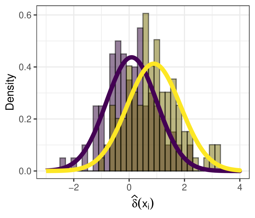
(a)

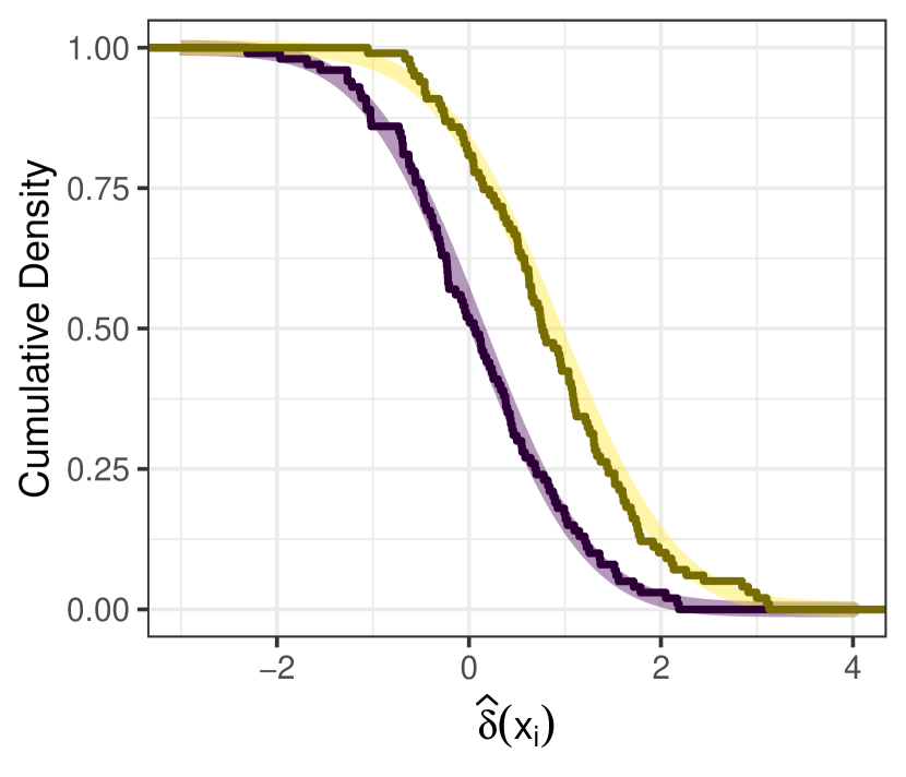
(b)

Figure 2: Illustrating the difference between estimating the true/false positive rate in Median Sweep and Continuous Sweep. In Figure (a), the histogram shows the distributions of the discriminant scores in the negative (purple) and the positive (yellow) class, where the corresponding coloured lines show the fitted Gaussians. In Figure (b), Median Sweep uses empirical cumulative distribution functions (step functions) to estimate the true/false positive rate, while Continuous Sweep uses the Gaussian cumulative distribution (continuous curves) to estimate the true/false positive rate.

Unlike for the functions of the true positive rate and the false positive rate, the function of the Classify-and-Count quantifier $\hat{\alpha}_{\text{CC}}(\theta,D_{\text{test}})$ cannot be estimated as a continuous, parametric curve. The full Classify-and-Count distribution is a mixture distribution with an unknown mixture parameter closely related to prevalence $\alpha$. Therefore, $\hat{\alpha}_{\text{CC}}(\theta,D_{\text{test}})$ remains a step-function for future calculations. Note that this approach differs from Kloos et. al [27], where the Classify-and-Count quantifier is estimated using kernel methods.

As illustrated in Fig. 3, $\hat{\alpha}_{\text{AC}}$ is a continuous function between any two discriminant scores occurring in $D_{\text{test}}$. On such an interval, $\hat{\alpha}_{\text{CC}}$ is constant and, consequently, the graph of $\hat{\alpha}_{\text{AC}}$ is continuous. For each jump in $\hat{\alpha}_{\text{CC}}$, we move to a new interval. For extreme discriminant scores $\theta$, the estimates in $\hat{\alpha}_{\text{AC}}$ have a high variance resulting in potentially extreme prevalence estimates. To address this issue, the second property of Median Sweep will be changed.

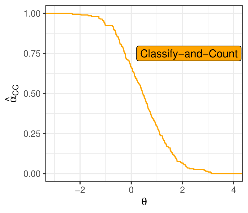
(a)

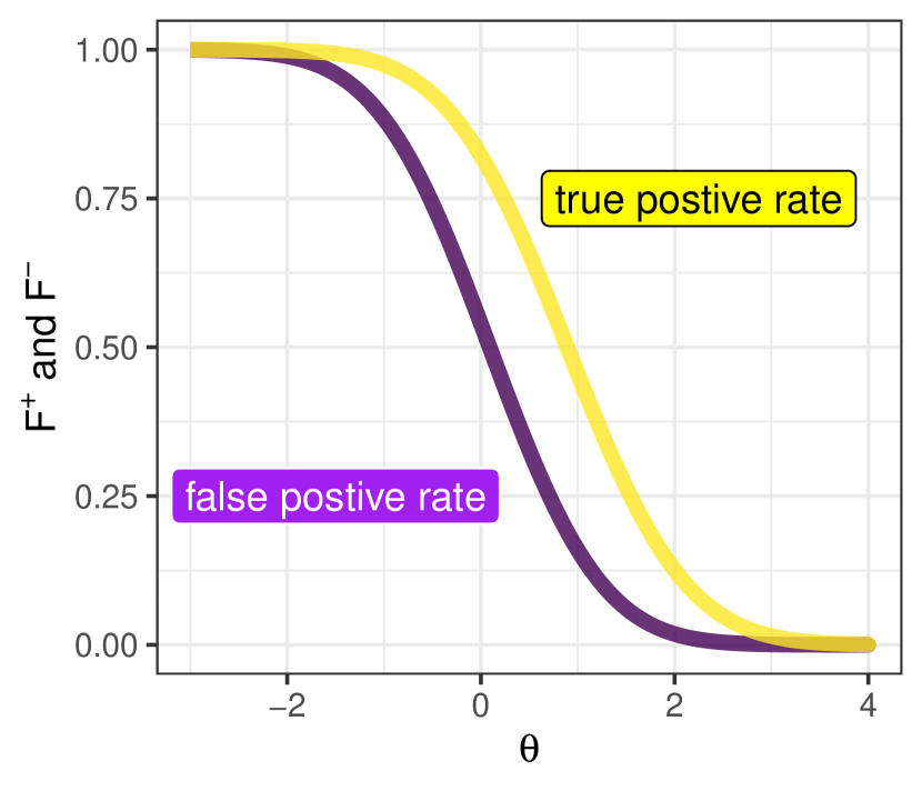
(b)

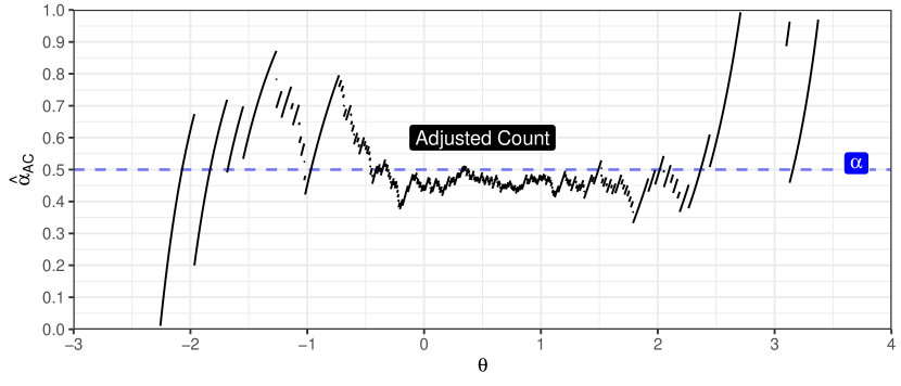
(c)

Figure 3: Using a Classify-and-Count function as a step function (Panel (a)) and the true and false positive rate as continuous functions (Panel (b)), the Adjusted-Count quantifier can estimate prevalence $\alpha$ at each $\theta$ (Panel (c)).

The second adjustment to Median Sweep regards the decision rule for discarding individual data points. As described in Section 2, Median Sweep only considers prevalence estimates at thresholds equal to discriminant scores occurring in $D_{\text{test}}$ for which the difference between $\hat{F}^{+}(\theta,D_{\text{test}})$ and $\hat{F}^{-}(\theta,D_{\text{test}})$ is greater or equal than $1/4$. This rule makes it hard to derive the variance of the mean or median prevalence estimate analytically, because the number of observations that pass the decision rule differs between test sets. Consequently, we need many computations conditioned on the number of observations that pass the decision rule, which is cumbersome to compute. Furthermore, the cut-off point of $1/4$ seems to have no mathematical justification and therefore may be improved, in two steps. First, instead of including or discarding prevalence estimates at only the discriminant scores occurring in $D_{\text{test}}$, i.e., a discrete set, Continuous Sweep considers all prevalence estimates for every $\theta$ on an entire interval. Second, instead of a fixed cutoff of $1/4$, the cutoff is considered a parameter, $p^{\Delta}$, which can be optimized (see Section 3.3). Therefore, the thresholds $\theta$ where $F^{+}(\theta,D_{\text{test}})-F^{-}(\theta,D_{\text{test}})=p^{\Delta}$ are defined as decision boundaries $\theta_{\text{l}}$ (left) and $\theta_{\text{r}}$ (right), and all the points between the decision boundaries are included in the final prevalence estimate . To obtain the decision boundaries, we solve the equation $F^{+}(\theta,D_{\text{test}})-F^{-}(\theta,D_{\text{test}})-p^{\Delta}=0$. In Fig. 4, the difference between Median Sweep and Continuous Sweep is illustrated, where in Median Sweep only the green dots are included in the final calculation for $\hat{\alpha}_{\text{MS}}$ whereas for continuous sweep all values within the decision boundary are included.

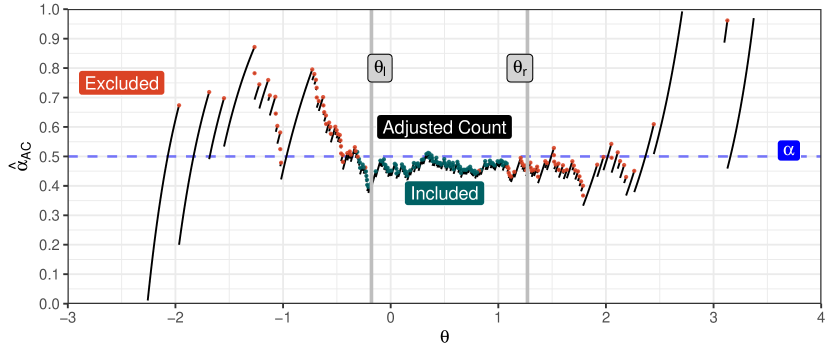
Figure 4: Example of discarding individual data points (red/green) against decision boundaries (grey, vertical). For Median Sweep, the green points are included in the prevalence calculation, while the red points are excluded. Continuous Sweep includes every $\theta$ between $\theta_{\text{l}}$ and $\theta_{\text{r}}$ in the calculations.

The third adjustment relates to the median. The median can only be computed analytically when the cumulative distribution function of $\hat{\alpha}_{\text{AC}}(\theta,D_{\text{train}},D_{\text{test}})$ between $\theta_{\text{l}}$ and $\theta_{\text{r}}$ is known. Because $\hat{\alpha}_{\text{AC}}(\theta,D_{\text{train}},D_{\text{test}})$ consists of many continuous functions in this parameter space that are collectively non-bijective, it is far-fetched to obtain its cumulative distribution function. As illustrated in Fig. 5, computing the mean analytically requires less effort, because it only includes the area under the curve. Every line segment between $\theta_{\text{l}}$ and $\theta_{\text{r}}$ can be calculated by integrating Eq. (15) with respect to $\theta$, resulting in a range of areas. The Continuous Sweep quantifier $\hat{\alpha}_{\text{CS}}$ is obtained by summing all areas between $\theta_{\text{l}}$ and $\theta_{\text{r}}$ divided by the distance between $\theta_{\text{l}}$ and $\theta_{\text{r}}$ as

$$\hat{\alpha}_{\text{CS}}(D_{\text{train}},D_{\text{test}}) =\frac{1}{\theta_{\text{r}}-\theta_{\text{l}}}\int_{\theta_{\text{l}}}^{\theta_{\text{r}}}\frac{\hat{\alpha}_{\text{CC}}(\theta,D_{\text{test}})-\hat{F}^{-}(\theta,D_{\text{train}})}{\hat{F}^{+}(\theta,D_{\text{train}})-\hat{F}^{-}(\theta,D_{\text{train}})}d\theta.$$ (16)

Eq. (16) cannot be evaluated in one calculation, because the curve exists of many continuous parts. The process on how to compute Eq. (16) is found in Algorithm (1). Note that the algorithm to calculate Continuous Sweep is different from Kloos et. al [27], because the Continuous Sweep quantifier has been improved since these working notes have been published.

Algorithm 1 Computing Continuous Sweep

1:Input: training data $D_{\text{train}}$ test data $D_{\text{test}}$, difference parameter $p^{\Delta}$.

2:Output: prevalence estimate $\hat{\alpha}_{\text{CS}}$

3:$\theta_{\text{l}},\theta_{\text{r}}\leftarrow$ ObtainDecisionBoundaries($D_{\text{train}},p^{\Delta}$)

4:ths $\leftarrow\verb|sort|(D_{\text{test}}[D_{\text{test}}\geq\theta_{\text{l}}\text{ \& }D_{\text{test}}\leq\theta_{\text{r}}])$

5:$N_{\text{ths}}\leftarrow$ length(ths)

6:A $\leftarrow$ length(ths $-1$)

7:for $i$ in $1,2,...,N_{\text{ths}}-1$ do

8:     A[i] $\leftarrow$ Integrate($\hat{\alpha}_{\text{AC}}(\theta,D_{\text{train}},D_{\text{test}})$, min = ths[i], max = ths[i+1], var = $\theta$)

9:end for

10:SumArea $\leftarrow$ sum(A)

11:return $\hat{\alpha}_{\text{CS}}=\frac{\text{SumArea}}{\theta_{\text{r}}-\theta_{\text{l}}}$

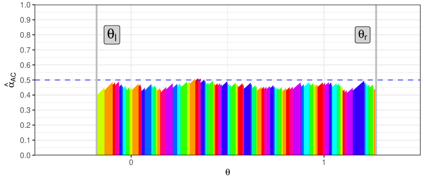
Figure 5: Example of using integrals to compute the prevalence using Continuous Sweep. The estimated prevalence is computed by summing the coloured areas divided by the difference between $\theta_{\text{l}}$ and $\theta_{\text{r}}$.

3.2 The bias and variance of Continuous Sweep

One of the main advantages of Continuous Sweep over Median Sweep is the ability to derive equations for the bias and variance, which in turn can be used to optimize the performance of both quantifiers. In this paper, we derive equations for the bias and variance of Continuous Sweep, given that the marginal distributions $F^{+}$ and $F^{-}$ are known. Given these assumptions, we first prove that Continuous Sweep is unbiased.

Theorem 1.

Assuming that $F^{+}$ and $F^{-}$ are known, the expected value of the Continuous Sweep quantifier $\hat{\alpha}_{\text{CS}}$ is equal to the true prevalence $\alpha$ and is therefore unbiased.

$$E[\hat{\alpha}_{\text{CS}}(\theta,D_{\text{test}})] =\alpha$$ (17)

Proof.

The expected value of Continuous Sweep is equal to

$$E\left[\hat{\alpha}_{\text{CS}}(\theta,D_{\text{test}})\right] =E\left[\frac{1}{\theta_{\text{r}}-\theta_{\text{l}}}\int_{\theta_{\text{l}}}^{\theta_{\text{r}}}\hat{\alpha}_{\text{AC}}(\theta,D_{\text{test}})d\theta\right]$$

$$=\frac{1}{\theta_{\text{r}}-\theta_{\text{l}}}E\left[\int_{\theta_{\text{l}}}^{\theta_{\text{r}}}\frac{\hat{\alpha}_{\text{CC}}(\theta,D_{\text{test}})-F^{-}(\theta)}{F^{+}(\theta)-F^{-}(\theta)}d\theta\right].$$ (18)

According to Fubini’s Theorem, we may exchange the integral and the expectation of Eq. (3.2) if the following holds:

$$E\left[\int_{\theta_{\text{l}}}^{\theta_{\text{r}}}\bigg{\lvert}\frac{\hat{\alpha}_{\text{CC}}(\theta,D_{\text{test}})-F^{-}(\theta)}{F^{+}(\theta)-F^{-}(\theta)}\bigg{\rvert}d\theta\right]<\infty.$$ (19)

The decision boundaries ensure that, for all $\theta$ between $\theta_{\text{l}}$ and $\theta_{\text{l}}$, $F^{+}(\theta)-F^{-}(\theta)\geq p^{\Delta}$. Furthermore, the parameters $\hat{\alpha}_{\text{CC}}(\theta,D_{\text{test}})$ and $F^{-}(\theta)$ are naturally bounded between $0$ and $1$, and $p^{\Delta}$ is a constant independent of $D_{\text{test}}$. Therefore, $\hat{\alpha}_{\text{AC}}(\theta,D_{\text{test}})$ is bounded between $\frac{-1}{p^{\Delta}}$ and $\frac{1}{p^{\Delta}}$ if $p^{\Delta}>0$, for all values of $\theta$ and all test sets $D_{\text{test}}$. Hence, for each $D_{\text{test}}$, it holds that $\int_{\theta_{\text{l}}}^{\theta_{\text{r}}}\bigg{\lvert}\frac{\hat{\alpha}_{\text{CC}}(\theta,D_{\text{test}})-F^{-}(\theta)}{F^{+}(\theta)-F^{-}(\theta)}\bigg{\rvert}d\theta\leq\frac{\theta_{\text{r}}-\theta_{\text{l}}}{p^{\Delta}}$. Therefore, Eq. (19) holds and Fubini’s theorem can be applied. As a result, the integral and expectation in Eq. (3.2) are interchangeable as

$$E\left[\hat{\alpha}_{\text{CS}}(\theta,D_{\text{test}})\right] =\frac{1}{\theta_{\text{r}}-\theta_{\text{l}}}\int_{\theta_{\text{l}}}^{\theta_{\text{r}}}E\left[\hat{\alpha}_{\text{AC}}(\theta,D_{\text{test}})\right]d\theta.$$ (20)

Assuming that the parameters of $F^{+}$ and $F^{-}$ for each value of $\theta$ are known, it follows that $D_{\text{test}}$ is the only stochastic variable in the expectation. Using Eq. (13) then yields

$$E\left[\hat{\alpha}_{\text{AC}}(\theta,D_{\text{test}})\right] =\frac{E[\hat{\alpha}_{\text{CC}}(\theta,D_{\text{test}})]-F^{-}(\theta)}{F^{+}(\theta)-F^{-}(\theta)}=\frac{\alpha\cdot(F^{+}(\theta)-F^{-}(\theta))}{F^{+}(\theta)-F^{-}(\theta)}=\alpha.$$ (21)

Hence, the expectation of the Adjusted-Count quantifier is the true prevalence irrespective of $\theta$. Then, it is straightforward to substitute Eq. (21) in Eq. (20), resulting in

$$E\left[\hat{\alpha}_{\text{CS}}(\theta,D_{\text{test}})\right] =\frac{1}{\theta_{\text{r}}-\theta_{\text{l}}}\int_{\theta_{\text{l}}}^{\theta_{\text{r}}}E\left[\hat{\alpha}_{\text{AC}}(\theta,D_{\text{test}})\right]d\theta$$

$$=\frac{1}{\theta_{\text{r}}-\theta_{\text{l}}}\int_{\theta_{\text{l}}}^{\theta_{\text{r}}}\alpha\text{ }d\theta=\frac{\alpha(\theta_{\text{r}}-\theta_{\text{l}})}{\theta_{\text{r}}-\theta_{\text{l}}}=\alpha.$$ (22)

This proves that $\hat{\alpha}_{\text{CS}}$ is unbiased. ∎

Because Continuous Sweep is unbiased, the mean squared error of the Continuous Sweep is equal to its variance, which we derive below.

Theorem 2.

The variance of Continuous Sweep is

$$V\left[\hat{\alpha}_{\text{CS}}\right] =\frac{2}{n_{\text{test}}(\theta_{\text{r}}-\theta_{\text{l}})^{2}}\int_{y=\theta_{\text{l}}}^{\theta_{\text{r}}}\int_{x=y}^{\theta_{\text{r}}}\frac{\alpha F^{+}(y)(1-F^{+}(x))+(1-\alpha)F^{-}(y)(1-F^{-}(x))}{(F^{+}(x)-F^{-}(x))(F^{+}(y)-F^{-}(y))}dxdy.$$ (23)

Proof.

The first step in computing the variance of Continuous Sweep is rewriting the variance in terms of expectations as

$$V\left[\hat{\alpha}_{\text{CS}}\right] =E\left[(\hat{\alpha}_{\text{CS}})^{2}\right]-E\left[\hat{\alpha}_{\text{CS}}\right]^{2}$$

$$=E\left[\left(\frac{1}{\theta_{\text{r}}-\theta_{\text{l}}}\int_{\theta=\theta_{\text{l}}}^{\theta_{\text{r}}}\hat{\alpha}_{\text{AC}}(\theta,D_{\text{test}})\text{ }d\theta\right)^{2}\right]-\alpha^{2},$$ (24)

by using Theorem 1 for computing the first moment. The second moment can be computed by expanding its expectation as

$$E\left[(\hat{\alpha}_{\text{CS}})^{2}\right] =E\left[\left(\frac{1}{\theta_{\text{r}}-\theta_{\text{l}}}\int_{x=\theta_{\text{l}}}^{\theta_{\text{r}}}\hat{\alpha}_{\text{AC}}(x,D_{\text{test}})\text{ }dx\cdot\frac{1}{\theta_{\text{r}}-\theta_{\text{l}}}\int_{y=\theta_{\text{l}}}^{\theta_{\text{r}}}\hat{\alpha}_{\text{AC}}(y,D_{\text{test}})\text{ }dy\right)\right]$$

$$=\frac{1}{(\theta_{\text{r}}-\theta_{\text{l}})^{2}}E\left[\left(\int_{x=\theta_{\text{l}}}^{\theta_{\text{r}}}\int_{y=\theta_{\text{l}}}^{\theta_{\text{r}}}\hat{\alpha}_{\text{AC}}(x,D_{\text{test}})\cdot\hat{\alpha}_{\text{AC}}(y,D_{\text{test}})\text{ }dxdy\right)\right]$$

Similar to Theorem (1), it can be proved that the integrand of Eq. (2) is uniformly bounded, because $0<(\theta_{\text{r}}-\theta_{\text{l}})^{2}<\infty$ and $0\leq\hat{\alpha}_{\text{AC}}(\theta,D_{\text{test}})\leq\frac{1}{(p^{\Delta})^{2}}$ for all $D_{\text{test}}$ and all $\theta$ in the relevant region. Hence, Fubini’s Theorem can be used once more to interchange the integral and the expectation as

$$E\left[(\hat{\alpha}_{\text{CS}})^{2}\right]=\frac{1}{(\theta_{\text{r}}-\theta_{\text{l}})^{2}}\int_{x=\theta_{\text{l}}}^{\theta_{\text{r}}} \int_{y=\theta_{\text{l}}}^{\theta_{\text{r}}}E\left[\hat{\alpha}_{\text{AC}}(x,D_{\text{test}})\cdot\hat{\alpha}_{\text{AC}}(y,D_{\text{test}})\right]dxdy.$$ (26)

Using the covariance rule $E[XY]=C[X,Y]+E[X]E[Y]$, the integral can be rewritten as an integral with a covariance as

$$E\left[(\hat{\alpha}_{\text{CS}})^{2}\right] =\frac{1}{(\theta_{\text{r}}-\theta_{\text{l}})^{2}}\int_{x=\theta_{\text{l}}}^{\theta_{\text{r}}}\int_{y=\theta_{\text{l}}}^{\theta_{\text{r}}}C\left[\hat{\alpha}_{\text{AC}}(x,D_{\text{test}})\cdot\hat{\alpha}_{\text{AC}}(y,D_{\text{test}})\right]$$

$$\qquad\qquad\qquad\qquad\qquad\qquad+E[\hat{\alpha}_{\text{AC}}(x,D_{\text{test}})]E[\hat{\alpha}_{\text{AC}}(y,D_{\text{test}})]dxdy$$ (27)

$$=\alpha^{2}+\frac{1}{(\theta_{\text{r}}-\theta_{\text{l}})^{2}}\int_{x=\theta_{\text{l}}}^{\theta_{\text{r}}}\int_{y=\theta_{\text{l}}}^{\theta_{\text{r}}}C\left[\hat{\alpha}_{\text{AC}}(x,D_{\text{test}})\cdot\hat{\alpha}_{\text{AC}}(y,D_{\text{test}})\right]dxdy.$$ (28)

If we substitute Eq. (28) in Eq. (24), we observe that the terms $\alpha^{2}$ cancel out. What remains is the covariance function, which can be simplified to

$$V\left[\hat{\alpha}_{\text{CS}}\right] =\frac{2}{(\theta_{\text{r}}-\theta_{\text{l}})^{2}}\cdot\int_{y=\theta_{\text{l}}}^{\theta_{\text{r}}}\int_{x=y}^{\theta_{\text{r}}}C\left[\hat{\alpha}_{\text{AC}}(x,D_{\text{test}}),\hat{\alpha}_{\text{AC}}(y,D_{\text{test}})\right]dxdy.$$ (29)

Similar to Theorem 1, the parameters of $F^{+}$ and $F^{-}$ are assumed to be known and can be written out of the covariance function as

$$V\left[\hat{\alpha}_{\text{CS}}\right] =\frac{2}{(\theta_{\text{r}}-\theta_{\text{l}})^{2}}\int_{y=\theta_{\text{l}}}^{\theta_{\text{r}}}\int_{x=y}^{\theta_{\text{r}}}\frac{C\left[\hat{\alpha}_{\text{CC}}(x,D_{\text{test}}),\hat{\alpha}_{\text{CC}}(y,D_{\text{test}})\right]}{(F^{+}(x)-F^{-}(x))(F^{+}(y)-F^{-}(y))}dxdy.$$ (30)

The Classify-and-Count quantifier counts the number of elements in $D_{\text{test}}$ that are larger or equal than $\theta$. $D_{\text{test}}$ is constructed as follows. One draws an i.i.d. sample of size $n_{\text{test}}^{+}$ from $F^{+}$, denoted as random variables $A_{1},A_{2},...,A_{n^{+}_{\text{test}}}$. Similarly, one draws another i.i.d. sample of size $n_{\text{test}}^{-}$ from $F^{-}$, denoted as random variables $B_{1},B_{2},...,B_{n^{-}_{\text{test}}}$. We assume that each $A_{i}$ is independent of each $B_{k}$. Using indices $x$ and $y$ for a pair of samples, the covariance function can be rewritten as

$$C[ \hat{\alpha}_{\text{CC}}(x,D_{\text{test}}),\hat{\alpha}_{\text{CC}}(y,D_{\text{test}})]=$$

$$C\left[\frac{1}{n_{\text{test}}}\left(\sum_{i=1}^{n_{\text{test}}^{+}}\mathbbm{1}\left\{A_{i}\geq x\right\}+\sum_{k=1}^{n_{\text{test}}^{-}}\mathbbm{1}\left\{B_{k}\geq x\right\}\right),\frac{1}{n_{\text{test}}}\left(\sum_{j=1}^{n_{\text{test}}^{+}}\mathbbm{1}\left\{A_{j}\geq y\right\}+\sum_{l=1}^{n_{\text{test}}^{-}}\mathbbm{1}\left\{B_{l}\geq y\right\}\right)\right]$$

$$= \frac{1}{n_{\text{test}}^{2}}\cdot C\left[\sum_{i=1}^{n_{\text{test}}^{+}}\mathbbm{1}\left\{A_{i}\geq x\right\}+\sum_{k=1}^{n_{\text{test}}^{-}}\mathbbm{1}\left\{B_{k}\geq x\right\},\sum_{j=1}^{n_{\text{test}}^{+}}\mathbbm{1}\left\{A_{j}\geq y\right\}+\sum_{l=1}^{n_{\text{test}}^{-}}\mathbbm{1}\left\{B_{l}\geq y\right\}\right].$$ (31)

The cross-products of the covariance function in Eq. (31) vanish because of our assumptions on independence. What remains is the equation

$$C[ \hat{\alpha}_{\text{CC}}(x,D_{\text{test}}),\hat{\alpha}_{\text{CC}}(y,D_{\text{test}})]=$$

$$\frac{1}{n_{\text{test}}^{2}}\cdot C\left[\sum_{i=1}^{n_{\text{test}}^{+}}\mathbbm{1}\left\{A_{i}\geq x\right\},\sum_{j=1}^{n_{\text{test}}^{+}}\mathbbm{1}\left\{A_{j}\geq y\right\}\right]+\frac{1}{n_{\text{test}}^{2}}\cdot C\left[\sum_{k=1}^{n_{\text{test}}^{-}}\mathbbm{1}\left\{B_{k}\geq x\right\},\sum_{l=1}^{n_{\text{test}}^{-}}\mathbbm{1}\left\{B_{l}\geq y\right\}\right]$$

$$=\frac{n_{\text{test}}^{+}}{n_{\text{test}}^{2}}C\left[\mathbbm{1}\left\{A_{1}\geq x\right\},\mathbbm{1}\left\{A_{1}\geq y\right\}\right]+\frac{n_{\text{test}}^{-}}{n_{\text{test}}^{2}}C\left[\mathbbm{1}\left\{B_{1}\geq x\right\},\mathbbm{1}\left\{B_{1}\geq y\right\}\right].$$ (32)

The covariances in Eq. (32) can be computed using the general rule $C[X,Y]=E[XY]-E[X]E[Y]$. Applying this rule combined with the indicator functions within the covariance function and the restriction that $x\geq y$ (review Eq. (29)) results in the following covariance function for the positives:

$$C\left[\mathbbm{1}\left\{A_{i}\geq x\right\},\mathbbm{1}\left\{A_{j}\geq y\right\}\right] =E[\mathbbm{1}\left\{A_{i}\geq x\right\}\cdot\mathbbm{1}\left\{A_{j}\geq y\right\}]-E[\mathbbm{1}\left\{A_{i}\geq x\right\}]\cdot E[\mathbbm{1}\left\{A_{j}\geq y\right\}]$$

$$=E[\text{min}(\mathbbm{1}\left\{A_{i}\geq x\right\},\mathbbm{1}\left\{A_{j}\geq y\right\})]-E[\mathbbm{1}\left\{A_{i}\geq x\right\}]\cdot E[\mathbbm{1}\left\{A_{j}\geq y\right\}]$$

$$=F^{+}(y)-F^{+}(x)\cdot F^{+}(y)=F^{+}(y)(1-F^{+}(x)).$$ (33)

Similarly, the following covariance function for the negatives can be derived:

$$C\left[\mathbbm{1}\left\{B_{k}\geq x\right\},\mathbbm{1}\left\{B_{l}\geq y\right\}\right] =F^{-}(y)-F^{-}(x)\cdot F^{-}(y)=F^{-}(y)(1-F^{-}(x)).$$ (34)

Substituting Eqs. (33) and (34) in Eq. (32) results in an equation for the covariance of two Classify-and-Count quantifiers at different thresholds $x$ and $y$:

$$C[\hat{\alpha}_{\text{CC}}(x,D_{\text{test}}),\hat{\alpha}_{\text{CC}}(y,D_{\text{test}})] =\frac{n_{\text{test}}^{+}}{n_{\text{test}}^{2}}F^{+}(y)(1-F^{+}(x))+\frac{n_{\text{test}}^{-}}{n_{\text{test}}^{2}}F^{-}(y)(1-F^{-}(x))$$

$$=\frac{\alpha}{n_{\text{test}}}F^{+}(y)(1-F^{+}(x))+\frac{1-\alpha}{n_{\text{test}}}F^{-}(y)(1-F^{-}(x)).$$ (35)

Finally, substituting Eq. (35) in Eq. (30) results in the variance of Continuous Sweep as

$$V\left[\hat{\alpha}_{\text{CS}}\right] =\frac{2}{n_{\text{test}}(\theta_{\text{r}}-\theta_{\text{l}})^{2}}\int_{y=\theta_{\text{l}}}^{\theta_{\text{r}}}\int_{x=y}^{\theta_{\text{r}}}\frac{\alpha F^{+}(y)(1-F^{+}(x))+(1-\alpha)F^{-}(y)(1-F^{-}(x))}{(F^{+}(x)-F^{-}(x))(F^{+}(y)-F^{-}(y))}dxdy.$$ (36)

This concludes the proof of the expressions for the variance of the Continuous Sweep. ∎

Now that we have derived the bias and variance of the Continuous Sweep quantifier, we will show how to use these results to derive an optimal value for the threshold $p^{\Delta}$.

3.3 Optimal threshold $p^{\Delta}$

The analytic expression for the variance of Continuous Sweep shows that its value is dependent on decision boundaries $\theta_{\text{l}}$ and $\theta_{\text{r}}$. Those two values are determined by $p^{\Delta}$, the minimum difference between the true and false positive rate of the data points to be included. As shown in Figure 6, a large value of $p^{\Delta}$ results in a small difference between $\theta_{\text{l}}$ and $\theta_{\text{r}}$, whereas a small value of $p^{\Delta}$ results in a large difference between $\theta_{\text{l}}$ and $\theta_{\text{r}}$.

A larger difference between the decision boundaries includes more, but potentially unreliable, data points in the prevalence estimate. Forman [10] proposed a threshold equal to $p^{\Delta}=1/4$, which we will call the traditional threshold. Minimizing Eq. (23), viewed as a function of $p^{\Delta}$, returns the optimal threshold $p^{\Delta}$, in the sense that it yields a prevalence estimate with minimal variance (and hence the minimal MSE due to Theorem 1).

The variance function of Eq. (23) has parameters that are often unknown in practice. For example, the prevalence $\alpha$ is a parameter in Eq. (23). Because the prevalence is unknown, one can use $\alpha=0.5$ as a plug-in estimate. We experimented that the prevalence has a negligible impact on the total variance and hence on the optimal $p^{\Delta}$. Therefore, the plug-in estimator of $\alpha=0.5$ can reliably be used in Eq. (23) and we do not include to maintain focus on this parameter. Moreover, the parameters of $F^{+}$ and $F^{-}$ may be estimated using $D_{\text{train}}$ if they are unknown. In that case, the optimal threshold can be estimated by using plug-in estimators for the parameters of $F^{+}$ and $F^{-}$ in Eq. (23). In our simulation studies, we use the optim function in R to approximate the optimal threshold numerically in this manner.

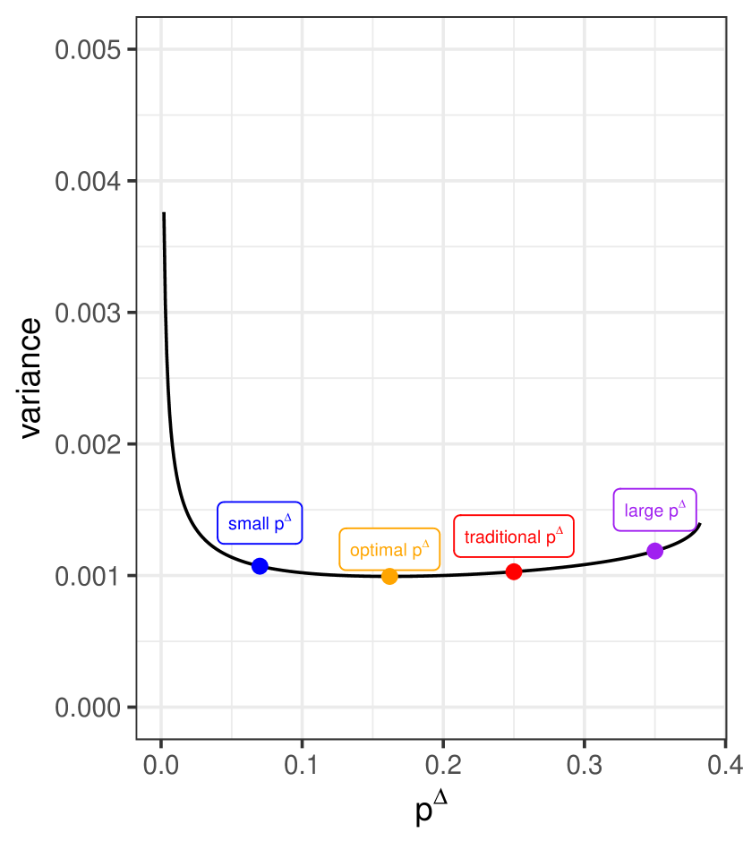
(a)

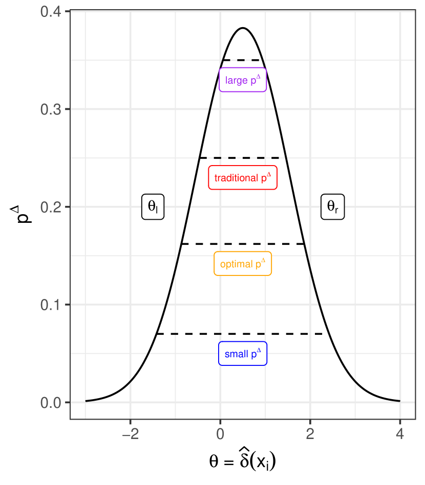
(b)

Figure 6: Panel (a) illustrates the theoretical variance at different $p^{\Delta}$ of the Continuous Sweep with a $D_{\text{test}}$ of size $1000$ and prevalence $\alpha=0.5$, where $F^{+}\sim N(1,1)$ and $F^{-}\sim N(0,1)$. Panel (b) illustrates the difference between $\theta_{\text{l}}$ and $\theta_{\text{r}}$ for each $p^{\Delta}$.

4 Simulation Study

In this section, we present three simulation studies to compare the performance of Continuous Sweep with Median Sweep. For the first study, discussed in Section 4.1, we assume that $F^{+}$ and $F^{-}$ follow a normal distribution with known parameters. We use the simulation study to compare Continuous Sweep and Median Sweep in the idealised situation where the assumptions correspond to the assumptions of Theorem 1 and 2. In practice, $F^{+}$ and $F^{-}$ have to be estimated from training data. The second simulation study examines the case where a normal model is fitted with normal data. Therefore, in the second simulation study, we still assume that $F^{+}$ and $F^{-}$ follow a normal distribution, but now their parameters are estimated from the data (resulting in $\hat{F}^{+}$ and $F^{-}$). Finally, in the third simulation study, we examine the case when the data are skew-normal distributed, and is fitted on two models using both normal data or skew-normal data.

4.1 Study 1: Known parameters for $F^{+}$ and $F^{-}$ using a normal distribution

Outline and design

This first simulation study assumes that the discriminant scores of the positive class follow a normal distribution $F^{+}$ with mean $\mu^{+}=1$ and a standard deviation $\sigma^{+}$, while the scores of the negative class follow a normal distribution $F^{-}$ with mean $\mu^{-}=0$ and a standard deviation of $\sigma^{-}$. Moreover, in this study we assume that the mean and standard deviation of classes are known. The test data $D_{\text{test}}$ contain a proportion $\alpha$ (prevalence) of discriminant scores sampled from $F^{+}$ and a proportion $1-\alpha$ of discriminant scores sampled from $F^{-}$.

Using $D_{\text{test}}$ and the known distributions of the discriminant scores, Continuous Sweep can estimate the prevalence with Algorithm 1. Estimating the prevalence using Median Sweep is described in Section 2. The decision boundaries $\theta_{l}$ and $\theta_{r}$ are determined using the known distributions $F^{+}$ and $F^{-}$. Consequently, we also use $F^{+}$ and $F^{-}$ in Eq. (16) instead of $\hat{F}^{+}$ and $\hat{F}^{-}$. To compute Median Sweep, $F^{+}$ and $F^{-}$ replace $p^{+}$ and $p^{-}$ in Eq. (11) and in the decision rule to obtain $\boldsymbol{\theta}_{\text{MS}}$.

As described in Section 3.3, the performance of Continuous Sweep, but also of Median Sweep, is dependent on $p^{\Delta}$. Hence, we apply the traditional value of $p^{\Delta}=1/4$ and the optimal $p^{\Delta}$ on both quantifiers, which results in a comparison between four quantifiers: 1) Optimal Continuous Sweep (O-CS), 2) Traditional Continuous Sweep (T-CS), 3) Optimal Median Sweep (O-MS), and 4) Traditional Median Sweep (T-MS).

We use a full-factorial design of four factors. The number of observations $n_{\text{test}}$ in $D_{\text{test}}$ is either $100$ or $1000$, which is mainly intended to investigate the relationship between sample size and variance. To investigate the relationship between the classifier and the quantifiers, the possible values of $\sigma^{+}$ and $\sigma^{-}$ are both set to $0.5$, $1$, and $1.5$. Last, the prevalence $\alpha_{\text{test}}$ can take values of $0.3$, $0.5$, and $0.9$ to examine whether the quantifiers have different bias and variance under either balanced or imbalanced data. The values of $\mu^{+}=1$ and $\mu^{-}=0$ are fixed across the simulation study. In summary, the simulation study has $2\times 3\times 3\times 3=54$ different situations. For each situation, we generate $1000$ test sets $D_{\text{test}}$ used to compute the prevalence estimates from the four quantifiers. With the prevalence estimates, we can estimate the bias, variance and mean squared error (MSE) for the four quantifiers under each of the $54$ situations. We show the results using a rank order in each of the $54$ situations, where rank $1$ indicates the quantifier with the lowest MSE in a situation and where rank $4$ indicates the quantifier with the largest MSE in a situation.

Table 1: The counts of ranks in MSE across the $54$ different situations for each each quantifier in the first simulation study. Rank $1$ is awarded to the quantifier with the lowest MSE, whereas rank $4$ is awarded to the quantifier with the largest MSE.

Rank by quantifier	1	2	3	4
Optimal Continuous Sweep	54	0	0	0
Traditional Continuous Sweep	0	35	12	7
Optimal Median Sweep	0	19	26	9
Traditional Median Sweep	0	0	16	38

Results

The results of the first simulation study are clear. Table 1 summarises the simulation study using ranks. O-CS has the lowest MSE of the four quantifiers in each of the $54$ situations. Moreover, T-CS is often second best, but it is outperformed by one or both Median Sweep quantifiers in some situations. Furthermore, O-MS performs often better than T-MS. The values for the bias, variance, and MSE for all quantifiers in each situation can be found in the online Appendix.

4.2 Study 2: Estimated parameters for $F^{+}$ and $F^{-}$ using a normal distribution

Outline and design

In the second simulation study, we make the assumption that the parameters of $F^{+}$ and $F^{-}$ are unknown and have to be estimated. Like the first simulation study, the positive discriminant scores are normally distributed with mean $\mu^{+}=1$, and standard deviation $\sigma^{+}$, and the negative discriminant scores are normally distributed with mean $\mu^{-}=0$, and standard deviation $\sigma^{-}$. The parameters of $\hat{F}^{+}$ and $\hat{F}^{-}$ can be estimated by maximum likelihood estimation. Accordingly, we can estimate decision boundaries $\theta_{l}$ and $\theta_{r}$ using the estimated $\hat{F}^{+}$ and $\hat{F}^{-}$. Again, we can use Algorithm 1 to compute the prevalence estimates of Continuous Sweep. Median Sweep estimates the true and false positive rate using empirical cumulative density functions $p^{+}$ and $p^{-}$.

In the second simulation study, we use the same $54$ settings for $n_{\text{test}}$, $\alpha_{\text{test}}$, $\mu^{+}$, $\mu^{-}$, $\sigma^{+}$, and $\sigma^{-}$. In addition, we add two extra variables $n_{\text{train}}$ and $\alpha_{\text{train}}$. We vary the size $n_{\text{train}}$ of the training set between $100$ and $1000$ and its prevalence $\alpha_{\text{train}}$ between $0.4$, $0.5$, and $0.6$. The reason why we vary little in $\alpha_{\text{train}}$ between training sets, is that extreme prevalence values return only a few data points for one class for small training sets, but we still want to investigate whether $\alpha_{\text{train}}$ has a large effect on the bias, variance and MSE of the quantifiers. The number of situations is therefore increased to $54\times 2\times 3=324$ situations.

Results

Table 2 summarizes the second simulation study. In general, the rank order is similar to the first simulation study, where O-CS performed the best most often, while T-MS performed often the worst. However, O-CS was not the single-best quantifier, as T-CS was occasionally ranked highest. In addition, the Median Sweep was never ranked as the best-performing quantifier. Similar to the full results of the first simulation study, all values for the bias, variance and MSE for all quantifiers in each situation can be found in the online Appendix.

Fig. 7 provides further insights into these results by showing when O-CS performs better than T-CS in certain situations. Specifically, O-CS performs the best when the class majority belonged to a class with small variance, when the training set was large, and when the test set was small.

Table 2: The distribution of ranks in MSE across the $324$ different situations for each quantifier in the first simulation study. Rank $1$ is awarded for the quantifier with the lowest MSE, whereas rank $4$ is awarded for the quantifier with the largest MSE.

Rank by quantifier	1	2	3	4
Optimal Continuous Sweep	209	60	31	24
Traditional Continuous Sweep	115	143	37	29
Optimal Median Sweep	0	65	175	84
Traditional Median Sweep	0	56	81	187

Figure 7: Decision tree in finding the best quantifier in a specific situation. Optimal Continuous Sweep (O-CS) is often better than Traditional Continuous Sweep (T-CS), especially when the underlying classifier has a high accuracy (low standard deviation of the discriminant scores in the majority class) and/or trained with enough data.

4.3 Study 3: Misfit on more complex distributions

Outline and design

Similar to the second simulation study, the third simulation study assumes that the parameters $\mu^{+}$, $\mu^{-}$, $\sigma^{+}$, and $\sigma^{-}$ of $F^{+}$ and $F^{-}$ are unknown and are estimated from training set $D_{\text{train}}$. However, instead of a normal distribution, we assume that the positive and negative labeled discriminant scores of $D_{\text{train}}$ and $D_{\text{test}}$ are i.i.d. sampled from a skew-normal distribution. In this simulation study, we investigate the robustness of Continuous Sweep under model misspecification. Additionally, we want to check how Continuous Sweep performs when the skew-normal distribution is well-specified.

Fitting Continuous Sweep with a skew-normal distribution takes substantially more time than fitting Continuous Sweep with a normal distribution. Therefore, we take a subset of the design given in the second simulation study. For all simulation studies, $D_{\text{train}}$ consists of $1000$ observations with prevalence $\alpha_{\text{train}}=0.5$. The test set $D_{\text{test}}$ can vary between $100$ and $1000$ observations, the standard deviations $\sigma^{+}$ and $\sigma^{-}$ can both take the values $0.5$ and $1.5$, and the test set prevalence $\alpha_{\text{test}}$ can vary between $0.3$, $0.5$, and $0.9$. This results in $2\times 2\times 2\times 3=24$ situations. Each of the 24 situations are fitted on three small simulation studies: the first study considers little skew in the data, the second study considers medium skew and the third study considers large skew.

To summarize, we compare in this simulation study the quantifiers Median Sweep (MS), Continuous Sweep with normal fit (CS (norm)), and Continuous Sweep with skew-normal fit (CS (skew)), all with an optimal (O) and a traditional (T) $p^{\Delta}$. The skewness of the data is either small, medium, or large, resulting in three small simulation studies on $24$ different situations of the data.

We fit Median Sweep and Continuous Sweep using the normal distribution in the same way as in the second simulation study. Continuous Sweep using the skew-normal distribution works similarly, but a additional shape parameter is required. We estimate the shape parameter using maximum likelihood estimation, since no analytic solution exists.

Results

Table 3 summarizes the results of the third simulation study. For each level of skewness, the Continuous Sweep quantifiers with skew-normal fit consistently outperform the other quantifiers. O-CS (norm) outperforms MS if the skew is small, but performs worse when the skew increases. In general, an optimal $p^{\Delta}$ performs better across the situations than a traditional $p^{\Delta}=1/4$ across all quantifiers and levels of skewness. Similar to the full results of the previous simulation studies, all values for the bias, variance and MSE for all quantifiers in each can be found in the online Appendix.

Table 3: The full-factorial design of the second simulation study. Each combination of the parameters is used to compute the bias, variance and RMSE of the Continuous Sweep with normal and skew-normal fit and Median Sweep.

	little skew (shape = 1)
Rank quantifier	1	2	3	4	5	6	avg
O-CS (skew)	21	1	2	0	0	0	1.21
T-CS (skew)	3	5	3	9	4	0	3.25
O-CS (normal)	0	12	4	6	2	0	2.92
T-CS (normal)	0	2	3	3	7	9	4.75
O-MS	0	4	11	1	7	1	3.58
T-MS	0	0	1	5	4	14	5.29
	medium skew (shape = 2)
O-CS (skew)	18	6	0	0	0	0	1.25
T-CS (skew)	6	7	4	5	2	0	2.58
O-CS (normal)	0	1	5	2	12	4	4.54
T-CS (normal)	0	0	2	4	4	14	5.25
O-MS	0	10	3	7	4	0	3.21
T-MS	0	0	10	6	2	6	4.14
	large skew (shape = 4)
O-CS (skew)	16	8	0	0	0	0	1.33
T-CS (skew)	8	8	4	4	0	0	2.17
O-CS (normal)	0	0	3	2	11	8	5.00
T-CS (normal)	0	0	2	1	7	14	5.38
O-MS	0	8	6	10	0	0	3.08
T-MS	0	0	9	7	6	2	4.04

4.4 Summary

We compared Continuous Sweep and Median Sweep by three simulation studies. The first simulation study showed that Continuous Sweep with an optimal threshold always outperforms Median Sweep assuming that the distributions for the positive and negative discriminant scores are normal with known parameters. The second simulation study showed that either Continuous Sweep with an optimal threshold or Continuous Sweep with the traditional threshold outperforms Median Sweep assuming that the distributions for the positive and negative discriminant scores are normal with unknown parameters. The third simulation study shows that Continuous Sweep outperformed Median Sweep if the distributions of the discriminant scores are correctly specified (skew-normal data with skew-normal model assumptions), but underperformed when the distributions of the discriminant scores are misspecified (skew-normal data with normal model assumptions).

5 Discussion

In this paper, we presented Continuous Sweep: a new quantifier that advances in both theory and performance in quantification learning. Through three simulation studies, we demonstrated that Continuous Sweep has a lower mean squared error than Median Sweep across various scenarios, which is a substantial contribution in the search of better quantifiers. Moreover, we derived analytic expressions for the bias, variance, and mean squared error for Continuous Sweep. They reveal its theoretical properties under a set of common assumptions and enable the optimal selection of the hyperparameter $p^{\Delta}$. To the best of our knowledge, it is the first theoretical contribution to the ensemble quantifiers in the group Classify, Count, and Correct.

In addition to our main conclusion (Section 4.4), we provide three recommendations based on our simulation results. First, we recommend using Continuous Sweep when the distributions of the discriminant scores can be estimated accurately or are known. For example, the (raw) discriminant scores from a logistic model become approximately normally distributed if the number of independent variables in the data is large enough. This can be verified by, for example, data exploration using QQ-plots or histograms. Second, regarding the threshold, the traditional one is preferred over the optimal threshold when uncertainty in the parameter estimates increases. In the case of normal distributed discriminant scores, we recommend to use the optimal threshold when the distribution of the discriminant scores can be estimated accurately or are known. The only exception is when the standard deviation in both classes is at least half the difference of the means in the discrimination scores and either the training set or test set has less than $1000$ observations. Then we recommend to use Continuous Sweep with the traditional threshold. Third, if we are unable to estimate the distribution of the discriminant scores accurately, we recommend to use Median Sweep instead of Continuous Sweep.

We suggest three possible future research directions regarding Continuous Sweep. First, we suggest to extend the derivations for the bias and variance of Continuous Sweep. In this paper, we assume that we know the true positive rate and false positive rate at each threshold, but we can extend these derivations to the case where we have to estimate the parameters for the distributions of these rates. This is substantially harder, but allows for a better estimate for the optimal threshold. Second, we suggest to do simulation studies that focus on other types of data set shift than prior-probability shift. For example, we could evaluate the performance of Continuous Sweep, and other quantifiers, on, for example, covariate shift where also the class-conditional distributions change over time. Last, we suggest to apply Continuous Sweep on real-world data. However, despite some recent improvements, the availability of benchmark data sets suitable to evaluate quantification methods is a serious issue in the field of quantification [6, 18].

References

- \bibcommenthead
- Forman [2008] Forman, G.: Quantifying counts and costs via classification. Data Min. Knowl. Discov. 17(2), 164–206 (2008) https://doi.org/10.1007/s10618-008-0097-y
- Rath et al. [2020] Rath, S., Tripathy, A., Tripathy, A.R.: Prediction of New Active Cases of Coronavirus Disease (COVID-19) Pandemic Using Multiple Linear Regression Model. Diabetes Metab. Syndr. 14(5), 1467–1474 (2020) https://doi.org/10.1016/j.dsx.2020.07.045
- Lakhan et al. [2020] Lakhan, R., Agrawal, A., Sharma, M.: Prevalence of Depression, Anxiety, and Stress During COVID-19 Pandemic. J. Neurosci. Rural Pract. 11(04), 519–525 (2020) https://doi.org/10.1055/s-0040-1716442
- Chaudhry et al. [2021] Chaudhry, H.N., Javed, Y., Kulsoom, F., Mehmood, Z., Khan, Z.I., Shoaib, U., Janjua, S.H.: Sentiment Analysis of Before and After Elections: Twitter Data of US Election 2020. Electronics 10(17), 2082 (2021) https://doi.org/10.3390/electronics10172082
- Beijbom et al. [2015] Beijbom, O., Edmunds, P.J., Roelfsema, C., Smith, J., Kline, D.I., Neal, B.P., Dunlap, M.J., Moriarty, V., Fan, T.-Y., Tan, C.-J., et al.: Towards Automated Annotation of Benthic Survey Images: Variability of Human Experts and Operational Modes of Automation. PloS One 10(7), 0130312 (2015) https://doi.org/10.1371/journal.pone.0130312
- González et al. [2017] González, P., Castaño, A., Chawla, N.V., Coz, J.J.: A Review on Quantification Learning. ACM Comput. Surv. 50, 74–17440 (2017) https://doi.org/10.1145/3117807
- Czaplewski and Catts [1992] Czaplewski, R.L., Catts, G.P.: Calibration of Remotely Sensed Proportion or Area Estimates for Misclassification Error. Remote Sens. Environ. 39(1), 29–43 (1992) https://doi.org/10.1016/0034-4257(92)90138-A
- Bross [1954] Bross, I.D.J.: Misclassification in 2X2 Tables. Biom. 10, 478 (1954) https://doi.org/10.2307/3001619
- Kuha and Skinner [1997] Kuha, J., Skinner, C.: Categorical Data Analysis and Misclassification. In: Surv. Meas. and Process Qual., pp. 633–670. John Wiley & Sons, Ltd, Chichester, UK (1997). Chap. 28. https://doi.org/10.1002/9781118490013.ch28
- Forman [2005] Forman, G.: Counting Positives Accurately Despite Inaccurate Classification. Springer (2005). https://doi.org/10.1007/11564096_55
- Dougherty [2013] Dougherty, G.: Pattern Recognition and Classification: An Introduction. Springer, New York (2013). https://doi.org/10.1007/978-1-4614-5323-9
- Moreno-Torres et al. [2012] Moreno-Torres, J.G., Raeder, T., Alaíz-Rodríguez, R., Chawla, N.V., Herrera, F.: A unifying view on dataset shift in classification. Pattern Recognit. 45, 521–530 (2012) https://doi.org/10.1016/j.patcog.2011.06.019
- Milli et al. [2013] Milli, L., Monreale, A., Rossetti, G., Giannotti, F., Pedreschi, D., Sebastiani, F.: Quantification Trees. In: 2013 IEEE 13th International Conference on Data Mining, pp. 528–536. IEEE, Dallas (2013). https://doi.org/10.1109/ICDM.2013.122
- Barranquero et al. [2013] Barranquero, J., González, P., Díez, J., Del Coz, J.J.: On the Study of Nearest Neighbor Algorithms for Prevalence Estimation in Binary Problems. Pattern Recognit. 46, 472–482 (2013) https://doi.org/10.1016/j.patcog.2012.07.022
- Esuli and Sebastiani [2015] Esuli, A., Sebastiani, F.: Optimizing Text Quantifiers for Multivariate Loss Functions. Trans. Knowl. Discov. Data 9(4), 1–27 (2015) https://doi.org/10.1145/2700406
- Saerens et al. [2002] Saerens, M., Latinne, P., Decaestecker, C.: Adjusting the Outputs of a Classifier to New a Priori Probabilities: A Simple Procedure. Neural Comput. 14(1), 21–41 (2002) https://doi.org/10.1162/089976602753284446
- King and Lu [2008] King, G., Lu, Y.: Verbal autopsy methods with multiple causes of death. Statist. Sci. 23(1), 78–91 (2008) https://doi.org/10.1214/07-STS247
- Schumacher et al. [2021] Schumacher, T., Strohmaier, M., Lemmerich, F.: A Comparative Evaluation of Quantification Methods (2021). https://doi.org/10.48550/arXiv.2103.03223
- Maletzke et al. [2019] Maletzke, A., Reis, D., Cherman, E., Batista, G.: DyS: A Framework for Mixture Models in Quantification. In: Proceedings of the AAAI Conference on Artificial Intelligence, vol. 33, pp. 4552–4560 (2019). https://doi.org/10.1609/aaai.v33i01.33014552
- Kloos et al. [2021] Kloos, K., Meertens, Q.A., Scholtus, S., Karch, J.D.: Comparing Correction Methods to Reduce Misclassification Bias. Springer (2021). https://doi.org/10.1007/978-3-030-76640-5_5
- Kloos [2021] Kloos, K.: A New Generic Method to Improve Machine Learning Applications in Official Statistics. Stat. J. of the IAOS 37(4), 1181–1196 (2021) https://doi.org/10.3233/sji-210885
- Tasche [2017] Tasche, D.: Fisher Consistency for Prior Probability Shift. J. Mach. Learn. Res. 18(95), 1–32 (2017) https://doi.org/10.5555/3122009.3176839
- Tasche [2021] Tasche, D.: Minimising Quantifier Variance Under Prior Probability Shift (2021). https://doi.org/10.48550/ARXIV.2107.08209
- Meertens et al. [2022] Meertens, Q.A., Diks, C.G.H., Herik, H.J., Takes, F.W.: Improving the Output Quality of Official Statistics Based on Machine Learning Algorithms. J. of Off. Stat 38(2), 485–508 (2022) https://doi.org/10.2478/jos-2022-0023
- González et al. [2017] González, P., Díez, J., Chawla, N., Coz, J.J.: Why is Quantification an Interesting Learning Problem? Prog. in Artif. Intell. 6, 53–58 (2017) https://doi.org/10.1007/s13748-016-0103-3
- Forman [2006] Forman, G.: Quantifying Trends Accurately despite Classifier Error and Class Imbalance. Association for Computing Machinery, New York, NY, USA (2006). https://doi.org/10.1145/1150402.1150423
- Kloos et al. [2022] Kloos, K., Meertens, Q.A., Karch, J.D.: UniLeiden at LeQua 2022: The First Step in Understanding the Behaviour of the Median Sweep Quantifier using Continuous Sweep. In: Working Notes of the 2022 Conference and Labs of the Evaluation Forum (CLEF 2022), Bologna, Italy (2022). https://ceur-ws.org/Vol-3180/paper-150.pdf