Advancing continual lifelong learning in neural information retrieval: definition, dataset, framework, and empirical evaluation

Abstract

Continual learning refers to the capability of a machine learning model to learn and adapt to new information, without compromising its performance on previously learned tasks. Although several studies have investigated continual learning methods for information retrieval tasks, a well-defined task formulation is still lacking, and it is unclear how typical learning strategies perform in this context. To address this challenge, a systematic task formulation of continual neural information retrieval is presented, along with a multiple-topic dataset that simulates continuous information retrieval. A comprehensive continual neural information retrieval framework consisting of typical retrieval models and continual learning strategies is then proposed. Empirical evaluations illustrate that the proposed framework can successfully prevent catastrophic forgetting in neural information retrieval and enhance performance on previously learned tasks. The results indicate that embedding-based retrieval models experience a decline in their continual learning performance as the topic shift distance and dataset volume of new tasks increase. In contrast, pretraining-based models do not show any such correlation. Adopting suitable learning strategies can mitigate the effects of topic shift and data augmentation.

[aff1]organization=Department of Computer Science, School of Science, Loughborough University,addressline=Epinal Way, city=Loughborough, postcode=LE11 3TU, state=Leicestershire, country=UK [aff2]organization=Department of Mathematical Sciences, School of Science, Loughborough University,addressline=Epinal Way, city=Loughborough, postcode=LE11 3TU, state=Leicestershire, country=UK

1 Introduction

1.1 Background and motivation

Information retrieval, a fundamental area of research within natural language processing, focuses on identifying and extracting relevant information from a collection of documents [1]. Information retrieval technologies have led to the development of various real-world applications, including search engines, question-answering systems, and e-commerce recommender platforms [2]. With the advancement of deep learning, neural network-based information retrieval approaches known as neural information retrieval (NIR) [1] have exhibited superior results. Earlier NIR models [3, 4, 5, 6, 7] were primarily based on word embedding methods, while more recent NIR models [8, 9] have utilised pretrained language models (PLMs) [10] for improved performance.

Most deep learning models are trained using a fixed dataset, known as the isolated learning paradigm [11]. However, in real-world information retrieval applications and systems, new information is constantly arriving. Taking a document retrieval system as an example, the internal neural ranking model trained on old information may struggle to accurately sort and recommend the latest content, as new articles are constantly injected into the system over time, potentially leading to suboptimal user experiences due to the presence of different topics in the new articles. Re-training a new model every time novel data emerges is deemed impractical [12, 13]. As a consequence, the continual learning paradigm strives to facilitate the seamless integration of new data streams into neural networks as they become available [14, 15]. The main challenge in continual learning is to avoid catastrophic forgetting, i.e. the problem that deep learning models tend to forget previously acquired knowledge when learning on new data [16, 17].

Most existing continual learning strategies are designed for classification tasks [18, 19]. There has been limited focus on continual learning in information retrieval [20, 21], and it is not yet clear how existing learning strategies perform in this field of information retrieval. Hence, the primary objective of this study is to bridge this research gap. Moreover, the performance of continual learning can be affected by two important factors: data volume and topic shift. Data volume, i.e. the size of the new dataset, can lead to varying degrees of catastrophic forgetting as the amount of data increases [22, 23, 24]. On the other hand, topic shift, i.e. similarity between new tasks and previously learned tasks, can also impact continual learning performance when the similarity varies [25, 26, 27]. However, the effect of these two factors on continual learning in information retrieval tasks has not been investigated. Therefore, this study aims to fill this gap.

1.2 Research objectives and contributions

Considering the aforementioned research gaps, this study proposes two-fold research objectives. The first objective aims to assess the impact of emerging new data on NIR and determine the most effective continual learning strategies for different NIR models. The second objective seeks to uncover how variations in data volume and topic shift influence information retrieval performance in the context of continual learning.

However, it is important to note that, as of the present time, a well-defined mathematical task formulation and a benchmark dataset for NIR in a continual learning context are still absent. This absence poses a challenge in achieving the aforementioned research objectives effectively. In this paper, significant groundwork is laid out, which includes a precise task definition, the establishment of a benchmark dataset, and the development of a comprehensive continual information retrieval framework. These foundational elements serve as prerequisites for the empirical evaluation of the two research objectives. In summary, the key contributions of this paper are as follows:

1. A definition for the continual learning paradigm in the context of neural information retrieval tasks, as currently, no such definition exists.

2. A new dataset, called Topic-MSMARCO, specifically designed for evaluating continual information retrieval tasks.

3. A novel framework named Continual Learning Framework for Neural Information Retrieval (CLNIR), which allows for diverse NIR models and learning strategies to be paired, thereby creating a large number of continual information retrieval methods.

4. An empirical evaluation of the performance of different continual learning strategies for various NIR models, as well as an investigation into the impact of topic shift distance and data volume on continual information retrieval performance.

The remainder of the paper is organized as follows: Section 2 provides an overview of existing continual learning strategies and their attempted application in the field of NIR, thus laying the foundations for the proposed research. Section 3 outlines the task formulation and the evaluation metrics used in this study. Section 4 presents the proposed CLNIR and its architecture. Section 5 details the proposed Topic-MSMARCO dataset and the experiments on evaluating the two research objectives. Lastly, Section 6 provides suggestions for future work.

2 Related work

This section provides an overview of existing research on continual learning strategies and their application to information retrieval tasks.

2.1 Continual learning strategies

According to a survey by Lange et al. [18], continual learning can be classified into three categories: regularization-based, replay-based, and parameter isolation methods.

Regularization-based strategies primarily employ penalty terms in loss functions to control parameter updates. A well-known example of this approach is Elastic Weight Consolidation (EWC) [28], which slows down learning on certain neural parameter weights based on their importance to previous tasks. Another algorithm in this category is Synaptic Intelligence (SI) [29], which computes per-synapse consolidation strength in an online fashion over the entire learning trajectory in parameter space. To prevent important knowledge related to previous tasks from being overwritten, the Memory Aware Synapses (MAS) strategy [30] stores important information in a separate memory during training on new tasks and uses a regularization term to encourage the model to learn new information without disrupting the important information stored in the memory module. Mazur et al. [31] introduced a regularization strategy that utilizes the Cramer-Wold distance between target layer distributions, representing both current and past information. The proposed approach effectively mitigates the issue of increasing memory consumption, which often arises in similar methods. Furthermore, Zhang et al. [32] developed a novel method called Lifelong language method with Adaptive Uncertainty Regularization (LAUR). By employing LAUR, a single BERT model can be dynamically adapted to accommodate diverse NLP tasks without compromising performance.

Replay-based approaches typically store samples from old tasks and retrain them in new tasks. One example of this approach is the incremental classifier and representation learning [33], which uses a herding-based step for prioritized exemplar selection, and only requires a small number of exemplars per class. Another replay-based method is Gradient Episodic Memory (GEM) [34], which uses a subset of observed examples to minimize negative backward transfer. Zhuang et al. [35] have proposed a continual learning technique that selects samples by combining various criteria such as distance to prototype, intra-class cluster variation, and classifier loss.

Parameter isolation methods allocate dynamic network parameters to incremental data or tasks. One example of this approach is Progressive Neural Networks [36], which prevent catastrophic forgetting by instantiating a new neural network for each task being solved. Another parameter isolation method is the Expert Gate [37] which addresses continual learning issues by adding a new expert model when a new task arrives or knowledge is transferred from previous models.

2.2 Attempts of continual learning in information retrieval

A limited number of studies have explored the application of continual learning in information retrieval tasks. Wang et al. [38] and Song et al. [39] demonstrated the impact of continual learning methods on multi-modal embedding spaces in cross-modal retrieval tasks. In the text modality, Lovón-Melgarejo et al. [20] investigated the catastrophic forgetting problem in neural ranking models for information retrieval and their experiments revealed that the effectiveness of neural ranking comes at the cost of forgetting. However, transformer-based models provided a good balance between effectiveness and memory retention; and EWC [28] effectively mitigated catastrophic forgetting while maintaining a good trade-off between multiple tasks. Gerald and Soulier [21] built a sequential information retrieval dataset using the MSMARCO dataset [40] with sentence embedding and evaluated two pretraining-based NIR models: Vanilla BERT [10] and MonoT5 [41]. Gerald and Soulier [21] also found that catastrophic forgetting does exist in information retrieval, but to a lesser extent compared to some classification tasks. Only a few studies have investigated the relationship between catastrophic forgetting and NIR, and exploration of continual learning strategies in NIR remains limited. Furthermore, it is unclear which strategies perform well for NIR tasks.

3 Continual NIR task definition and evaluation metrics

3.1 Task definition

A continual neural information retrieval task is a specific type of continual learning task that involves a model that is able to retrieve relevant information from a continuously growing set of queries and documents.

• Let $D$ be a finite set of documents.

• Let $Q$ be a finite set of queries.

• Let $D(q)\subseteq D$ be the collection of documents related to a query $q\in Q$.

• Let $Y\coloneqq\{\langle q,d\rangle\mid q\in Q,d\in D(q)\}$ be the set of ground-truth relevance scores, where $\langle q,d\rangle$ represents the relevance score between $q$ and $d$. Relevance scores can be either a discrete value (“relevant” or “irrelevant”) or a continuous value (degree of relevance, e.g. between 0 and 1).

• Let $\mathbf{X}\coloneqq(Q,D,Y)$ and $\mathbf{X}^{\prime}\coloneqq(Q^{\prime},D^{\prime},Y^{\prime})$ be the training set and test set for neural information retrieval, respectively. The training set $\mathbf{X}$ is used to train the model; the test set $\mathbf{X}^{\prime}$ is used to evaluate the performance of a neural information retrieval model.

• Let $\mathcal{X}\coloneqq\{(\mathbf{X}_{1},\mathbf{X}^{\prime}_{1}),\dotsc,(\mathbf{X}_{T},\mathbf{X}^{\prime}_{T})\}$ be a sequential dataset for continual neural information retrieval that consists of $T$ tasks, where suitable subscripts have now been added to all the quantities defined above. The $t$th task consists of a training set $\mathbf{X}_{t}\coloneqq(Q_{t},D_{t},Y_{t})$ and a test set $\mathbf{X}^{\prime}_{t}\coloneqq(Q_{t}^{\prime},D_{t}^{\prime},Y_{t}^{\prime})$.

The continual neural information retrieval task requires parameters $\theta$ of a neural information retrieval model $\mathcal{R}(\theta)$ to be learned from a series of training sets in $\mathcal{X}$, one at a time. Starting with some initial parameters $\theta_{0}$, when a new training set $\mathbf{X}_{t}$ is fed into $\mathcal{R}(\theta_{t-1})$, the parameter $\theta_{t-1}$ is updated to $\theta_{t}$ by learning the samples in $\mathbf{X}_{t}$. Then, the updated model $\mathcal{R}(\theta_{t})$ is applied to all test sets $\mathbf{X}^{\prime}_{s}$ to yield sets of predicted relevance scores, $\smash{\hat{Y}_{t,s}^{\prime}\coloneqq\{\langle q,d\rangle_{t}|q\in Q_{s}^{\prime},d\in D_{s}^{\prime}(q)\}}$. Here, $\smash{\langle q,d\rangle_{t}}$ is the relevance score between query $q$ and document $d$ predicted by $\mathcal{R}(\theta_{t})$.

Finally, classical information retrieval metrics such as mean reciprocal recall or mean average precision then compute performance scores $P_{t,s}$ based on $Y_{s}^{\prime}$ and $\hat{Y}_{t,s}^{\prime}$. The choice of evaluation metric is flexible and depends on the specific retrieval scenatio [42, 43].

Figure 1 provides an example of a continual neural information retrieval task. It illustrates how the model adapts to a continuously growing set of queries and documents and continually records its performance on multiple test sets over time.

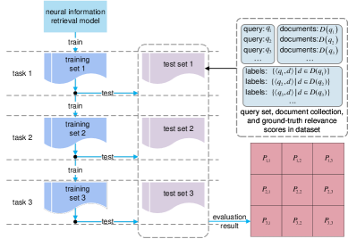
Figure 1: An example diagram of continual neural information retrieval with 3 tasks ($T=3$). The neural information retrieval model is initially trained on the training set of task 1 and then tested on all three test sets to generate $P_{1,1}$, $P_{1,2}$, and $P_{1,3}$. After training on the set for task 2, $P_{2,1}$, $P_{2,2}$, and $P_{2,3}$ will be generated. Finally, upon completion of task 3, the model will produce $P_{3,1}$, $P_{3,2}$, and $P_{3,3}$

3.2 Metrics for evaluating the performance of continual NIR models

The average evaluation performance of $\mathcal{R}(\theta_{T})$ (the retrieval model after learning all tasks) is

$$P_{\mathrm{final}}\coloneqq\frac{1}{T}\sum_{t=1}^{T}P_{T,t}.$$ (1)

To further explore the fine-grained continual learning performance of information retrieval, this study introduces backward transfer (BWT) and forward transfer (FWT) [34, 44] into the information retrieval scenario.

The backward transfer score, $\mathit{BWT}$, measures the influence that learning a task has, on average, on the performance of previous tasks:

$$\mathit{BWT}\coloneqq\frac{2}{T(T-1)}\sum_{t=2}^{T}\sum_{s=1}^{t}(P_{t,s}-P_{s,s}).$$ (2)

A negative score, $\mathit{BWT}<0$, indicates the average performance reduction of the previous test sets on newly trained tasks. Conversely, $\mathit{BWT}\geq 0$ indicates an absence of catastrophic forgetting.

The forward transfer score, $\mathit{FWT}$, measures the influence that learning a task has on the performance of future tasks:

$$\mathit{FWT}\coloneqq\frac{2}{T(T-1)}\sum_{t=1}^{T-1}\sum_{s=t+1}^{T}P_{t,s}.$$ (3)

A large value of $\mathit{FWT}$ indicates that the model performs well on test sets of unlearned tasks; a small value of $\mathit{FWT}$ indicates that the model is not able to effectively transfer knowledge from previous tasks to new ones.

4 Proposed CLNIR framework architecture

This section introduces the proposed Continual Learning Framework for Neural Information Retrieval (CLNIR). Inspired by a prior continual learning framework for classification tasks [45], the CLNIR framework allows for flexibility by decoupling the selection and implementation of the NIR model from the choice of learning strategy. The architecture of the proposed CLNIR framework is depicted in Figure 2. It consists of a learning strategy pool, a neural ranking model pool, and an agent model that performs NIR tasks.

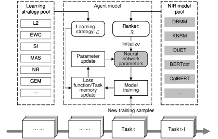
Figure 2: The CLNIR framework architecture.The NIR models and learning strategies mentioned will be explained in Sections 4.2 and 4.3 respectively.

4.1 Agent model

Algorithm 1 shows the workflow of the CLNIR framework. Line 1 initialises the agent model of the CLNIR framework with a designated NIR model (ranker $\mathcal{R}$), learning strategy ($\mathcal{L}$) and a loss function ($\ell$). The neural parameters within $\mathcal{R}$ are the optimization target of $\ell$. When new training samples are fed into CLNIR, $\mathcal{R}$ first learns the new data, similar to non-incremental learning tasks (Line 5). The CLNIR framework allows for two types of learning strategies:

• For regularization-based strategies (i.e. $\mathcal{L}\in\mathit{regularization}$), Line 7 lets the agent model generate a new regularization item, $\Omega_{t}$, which measures the importance of the different components of $\theta_{t}$. Line 8 then updates the loss function to account for the modified regularization term. A number of suitable regularization-based strategies will be described in Section 4.3.1.

• For replay-based strategies ($\mathcal{L}\in\mathit{replay}$), Line 10 first initializes an empty memory set, $\mathbf{M}$, when processing the first task. Line 11 then updates the memory set from the current training set using certain replay rules. For certain replay-based strategies, the loss function or the training set for the next task then need to be updated based on $\mathbf{M}$ (Lines 12–13). A number of suitable replay-based strategies will be described in Section 4.3.2.

After the training process, Line 14 updates the agent model; Lines 15–18 then send all test sets into the updated agent model to generate performance scores. Finally, Lines 19–21 calculate evaluation metrics from the performance scores as discussed in Section 3.2.

input : continual information retrieval agent model $\mathcal{A}$;

neural ranker $\mathcal{R}$ with initial parameter $\theta_{0}$;

learning strategy $\mathcal{L}$;

loss function $\ell$;

sequential NIR dataset $\mathcal{X}$ with $T$ tasks;

output : $\mathit{BWT}$; $\mathit{FWT}$; $P_{\mathrm{final}}$;

1 initialize agent model: $\mathcal{A}_{0}\leftarrow\mathcal{A}(\mathcal{R}(\theta_{0}),\mathcal{L})$;

2 initialize $U$ as an empty list;

3 initialize $V$ as an empty list;

4 for $t\leftarrow 1$ to $T$ do

5       $\theta_{t}\leftarrow$ Train($\mathcal{A}_{t-1}$, $\mathbf{X}_{t}$);

6       if $\mathcal{L}\in\mathit{regularization}$ then

7            

8            $\Omega_{t}\leftarrow$ CalculateParameterImportance($\mathbf{X}_{t},\theta_{t},\Omega_{t-1},\mathcal{L}$);

9             $\ell\leftarrow$ UpdateLossFunction($\ell$, $\Omega_{t}$);

10            

11      if $\mathcal{L}\in\mathit{replay}$ then

12            if $t=0$ then initialize memory set $\mathbf{M}$ an empty list;

13             $\mathbf{M}\leftarrow$ UpdateTaskMemory($\mathbf{X}_{t}$, $\mathbf{M}$);

14             $\ell\leftarrow$ UpdateLossFunction($\ell$, $\mathbf{M}$);

15             $\mathbf{X}_{t+1}\leftarrow$ UpdateNextTrainingData($\mathbf{X}_{t}$, $\mathbf{M}$);

16            

17      update agent model: $\mathcal{A}_{t}\leftarrow\mathcal{A}(\mathcal{R}(\theta_{t}),\mathcal{L})$;

18       for $s\leftarrow 1$ to $T$ do

19             $P_{t,s}\leftarrow$ Test($\mathcal{A}_{t}$, $\mathbf{X}^{\prime}_{s}$);

20             if $s\leq t$ then append $P_{t,s}$ to $U$;

21             else append $P_{t,s}$ to $V$;

22            

23      

24calculate $P_{\mathrm{final}}$ based on (1) and $U$;

25 calculate $\mathit{BWT}$ based on (2) and $U$;

calculate $\mathit{FWT}$ based on (3) and $V$. 

Algorithm 1 Continual neural information retrieval

4.2 NIR model pool

The proposed CLNIR framework consists of three state-of-the-art embedding-based methods and two pretraining-based methods. However, researchers who adopt the proposed framework can include other models.

4.2.1 Embedding based NIR models

DRMM. Deep Relevance Matching Models (DRMMs) [4] are interaction-based NIR models. Their architecture is depicted in Figure 3(a). Given a query text $q$ and a candidate document $d$, the DRMM model tokenizes the texts into fixed-length tokens $\mathbf{w}_{q}$ and $\mathbf{w}_{d}$, and generates corresponding masks $\mathbf{m}_{q}$ and $\mathbf{m}_{d}$. The tokens are then input into an embedding layer, and the resulting embedding matrices are masked by $\mathbf{m}_{q}$ and $\mathbf{m}_{d}$. The produced matrices for $q$ and $d$ can be represented as $\mathbf{E}_{q}\in\mathbb{R}^{\mathit{l}(q)\times n}$ and $\mathbf{E}_{d}\in\mathbb{R}^{\mathit{l}(d)\times n}$, respectively, where $\mathit{l}(q)$ and $\mathit{l}(d)$ represent the lengths of the query and document, respectively, and $n$ is the embedding dimension. The query representation is obtained by dividing $\mathbf{E}_{q}$ by its matrix norm, while the document representation is obtained from $\mathbf{E}_{d}$ in the same manner. Both representation matrices have the same dimensions as their corresponding embedding matrices.

The relevance between query representation and document representation is determined based on the cosine matrix similarity and tensor histogram. The cosine matrix $M_{\mathrm{cos}}\in\mathbb{R}^{\mathit{l}(q)\times\mathit{l}(d)}$ is obtained by taking the product of query representation and the transpose of document representation. Then, each row in $M_{\mathrm{cos}}$ is sorted into equal width ($b$) by a histogram function, resulting in a transformed matrix $M_{\mathrm{his}}\in\mathbb{R}^{\mathit{l}(q)\times b}$, where $b$ is the number of bins. Next, a series of linear and hyperbolic tangent (Tanh) layers are used to compress $M_{\mathrm{his}}$ and $\mathbf{E}_{q}$ into a relevance score vector $M_{\mathrm{rel}}\in\mathbb{R}^{\mathit{l}(q)}$ and a query gate vector $M_{\mathrm{gate}}\in\mathbb{R}^{\mathit{l}(q)}$, respectively. Finally, the relevance score is obtained by summing the element-wise product of $M_{\mathrm{rel}}$ and $M_{\mathrm{gate}}$.

KNRM. The architecture of Kernel-based Neural Ranking Models (KNRMs) [5] is shown in Figure 3(b). Similar to DRMM, their input includes tokens $\mathbf{w}_{q}$ and $\mathbf{w}_{d}$, and masks $\mathbf{m}_{q}$ and $\mathbf{m}_{d}$. Then tokens $\mathbf{w}_{q}$ and $\mathbf{w}_{d}$ are sent into an embedding layer to acquire query and document embeddings $\mathbf{E}_{q}$ and $\mathbf{E}_{d}$, which have the same shape as embedding matrices of DRMM. After normalization, $\mathbf{E}_{q}$ and $\mathbf{E}_{d}^{\mkern-1.5mu\mathsf{T}}\in\mathbb{R}^{n\times\mathit{l}(d)}$ are multiplied to an interaction matrix $M_{\mathrm{inter}}\in\mathbb{R}^{\mathit{l}(q)\times\mathit{l}(d)}$.

The $k$-kernel pooling function is then applied to $M_{\mathrm{inter}}$ to create a kernel pooling tensor $M_{\mathrm{pool}}\in\mathbb{R}^{\mathit{l}(q)\times\mathit{l}(d)\times k}$, where $k$ is the kernel size. The $M_{\mathrm{pool}}$ is multiplied with $\mathbf{m}_{d}$ to block unnecessary information, and then reduced to one dimensional $M^{\prime}_{\mathrm{pool}}\in\mathbb{R}^{\mathit{l}(q)\times k}$ by summing the elements in the second dimension. The tensor $M^{\prime}_{\mathrm{pool}}$ is then multiplied with $\mathbf{m}_{q}$ to block further unnecessary information and reduced to one dimensional $M^{\prime\prime}_{\mathrm{pool}}\in\mathbb{R}^{k}$ by summing the elements in the first dimension. Finally, $M^{\prime\prime}_{\mathrm{pool}}$ is processed by a feed-forward and sigmoid layer to produce a final relevance score.

DUET. The Duet [6] architecture consists of both a local model and a distributed model. The local model uses a local representation to match the query and document, while the distributed model uses learned distributed representations for the same purpose. The architecture of Duet is shown in Figure 3(c). In contrast to DRMM and KNRM, Duet includes an additional term frequency-inverse document frequency (TF-IDF) module to initialize a local distribution model $M_{\mathrm{local}}\in\mathbb{R}^{\mathit{l}(q)\times\mathit{l}(d)}$. Each element $w_{i}^{j}\in M_{\mathrm{local}}$ represents the TF-IDF score for the $i$th term in $q$ and the $j$th word in $d$ if the two terms are the same. The TF-IDF matrix is then reduced to one dimension, a vector $M^{\prime}_{\mathrm{local}}\in\mathbb{R}^{n}$ for the local representation.

In parallel, the embeddings of the query $\mathbf{E}_{q}\in\mathbb{R}^{\mathit{l}(q)\times n}$ and documents $\mathbf{E}_{d}\in\mathbb{R}^{\mathit{l}(d)\times n}$ are processed through one-dimensional convolutional and max-pooling layers to obtain one-dimensional representations $M_{q}\in\mathbb{R}^{n}$ and $M_{d}\in\mathbb{R}^{n\times c}$, respectively, where $c$ represents the output channel. The product of $M_{q}$ and $M_{d}$ is then added to $M^{\prime}_{\mathrm{local}}$ to generate a relevance score.

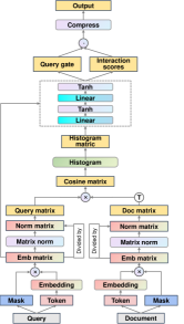
(a) DRMM.

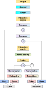
(b) KNRM.

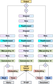
(c) DUET.

Figure 3: Architectures of word embedding based NIR models.

4.2.2 Pretraining based NIR models

BERTdot. BERT with Dot Productions (BERTdot) [46] is a direct application of the BERT model [10]. Its architecture is shown in Figure 4(a). A BERT tokenizer processes the query text $q$ and document text $d$ to extract tokens and masks, which are then input into the BERT encoding layer to generate text representation vectors. BERTdot uses the pooled vectors for query and document representation, denoted as $\mathbf{B}_{q}\in\mathbb{R}^{n}$ and $\mathbf{B}_{d}\in\mathbb{R}^{n}$, where $n$ is typically set to 768, the default hidden size of BERT. To calculate the dot product between these representations, they are expanded to $\mathbf{B}_{q}\in\mathbb{R}^{1\times n}$ and $\mathbf{B}_{d}\in\mathbb{R}^{n\times 1}$. The resulting output vector is then condensed to a scalar to represent the relevance score.

ColBERT. The Contextualized Late Interaction over BERT (ColBERT) model [9] encodes queries and documents separately and calculates the query-document similarity using a late interaction architecture, as shown in Figure 4(b). In contrast to BERTdot, the query and document representations, $\mathbf{B}_{q}\in\mathbb{R}^{\mathit{l}(q)\times n}$ and $\mathbf{B}_{d}\in\mathbb{R}^{\mathit{l}(d)\times n}$, respectively, are two-dimensional tensors encoded from the BERT architecture. The query representation and the transposed document representation are multiplied to obtain an interaction matrix $M_{\mathrm{inter}}\in\mathbb{R}^{\mathit{l}(q)\times\mathit{l}(d)}$. The maximum value in the last dimension of $M_{\mathrm{inter}}$ is then taken to represent the query term similarity score $M_{q}\in\mathbb{R}^{\mathit{l}(q)}$. Finally, all the similarity scores are summed to generate the final relevance score.

(a) BERTdot.

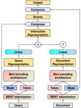
(b) ColBERT.

Figure 4: Architectures of pre-trained NIR models.

4.3 Learning strategies pool

In a real-world retrieval scenario, the amount of emerging data is vast (potentially infinite), making it unrealistic to employ parameter isolation strategies that demand a separate parameter space for every new dataset. While replay-based methods also face this challenge, it is possible to establish a fixed memory space of adequate size. Regularization-based strategies, on the other hand, are generally not influenced by the number of tasks, therefore, the learning strategy pool considered in this study encompasses both the widely used regularization-based and replay-based methods.

4.3.1 Regularization strategies for NIR

Let $\mathbf{x}=\langle\mathbf{q},\mathbf{pos},\mathbf{neg}\rangle$ be a batch of pairwise ranking samples for the current model input, where $\mathbf{q}$ represents a batch of queries, $\mathbf{pos}$ and $\mathbf{neg}$ represent the documents relevant and irrelevant to the queries in $\mathbf{q}$, respectively. Regularization-based strategies aim to control parameter updates with a penalty item in the loss function. The resulting penalized loss function is:

$$\ell(\mathbf{x};\theta)=\ell^{\prime}(\mathbf{x};\theta)+\lambda\sum_{i}(\theta^{i}-\vartheta^{i})^{2}\times\Omega^{i},$$ (4)

where $\lambda>0$ is the importance coefficient; $\vartheta=(\vartheta^{i})$ is the current value of the parameter $\theta=(\theta^{i})$; $\Omega=(\Omega^{i})$ is a regularization item obtained from the previous task to measure the importance of the $i$th parameter in $\theta$. Then, to train $x$ pairwise, a margin ranking loss is used for loss calculation. That is, $\ell^{\prime}(\mathbf{x};\theta)$ is the margin ranking loss function, defined as:

$$\ell^{\prime}(\mathbf{x};\theta)=\max\{0,-y(\mathcal{R}(\mathbf{q},\mathbf{pos};\theta)-\mathcal{R}(\mathbf{q},\mathbf{neg};\theta))+\mathit{margin}\}.$$ (5)

Here, $\mathcal{R}(\mathbf{q},\mathbf{pos};\theta)$ calculates the relevance scores between $\mathbf{q}$ and $\mathbf{pos}$, while $\mathcal{R}(\mathbf{q},\mathbf{neg};\theta)$ calculates the scores between $\mathbf{q}$ and $\mathbf{neg}$; $\mathit{margin}$ is a parameter to control the minimal difference between two ranking scores; and $y$ is a constant value. The difference between various regularization strategies lies in the addition of distinct regularization items in the loss function. The following are some methods used to implement these regularization items.

L2. The L2 strategy is a direct application of L2-regularization. The parameter importance is set to a constant to keep every parameter equal in importance:

$$\Omega^{i}=1.$$ (6)

EWC and EWCol. The Elastic Weight Consolidation (EWC) [28] strategy calculates the parameter importance based on the parameter gradient with the Fisher information matrix. After all samples in the training set $\mathbf{X}$ has been learned, a subset $\mathbf{X}^{*}$, of $K$ training samples from $\mathbf{X}$, called Fisher samples, is chosen to build the Fisher information matrix. Then $\mathbf{X}^{*}$ can be organized pairwise and the accumulated gradients generated from pairwise samples are used as parameter importance. The $k$th Fisher sample is denoted as $x_{k}^{*}=\langle q_{k}^{*},pos_{k}^{*},neg_{k}^{*}\rangle$. The average square of the gradients of each parameter is used as the regularization item for the next task. That is, if $\vartheta$ is the current parameter, set the regularisation item to

$$\Omega^{i}=\frac{1}{K}\sum_{k=1}^{K}\mathbf{G}^{i}(x_{k}^{*};\vartheta)^{2},$$ (7)

where

$$\mathbf{G}^{i}(x;\vartheta)=\frac{\partial\ell^{\prime}(x;\vartheta)}{\partial\vartheta^{i}}.$$ (8)

For Elastic Weight Consolidation in the Online Paradigm (EWCol), the previously accumulated importance factors will be added to the new ones:

$$\Omega^{i}\leftarrow\Omega^{i}+\frac{1}{K}\sum_{k=1}^{K}\mathbf{G}^{i}(x_{k};\vartheta)^{2}.$$ (9)

SI. The Synaptic Intelligence (SI) [29] strategy uses an importance measure to reflect the past credits for improvements of the regularized loss function for each parameter. Before training on a new batch $\mathbf{x}_{k}$, given the current parameter value $\vartheta_{k-1}$, with the convention that $\vartheta_{0}=\vartheta$ is the parameter learned at the end of the previous task and $\vartheta_{K}=\theta$ is the new parameter at the end of the current task. Then SI updates the parameter from $\vartheta_{k-1}$ to $\vartheta_{k}$ by learning $\mathbf{x}_{k}$ with a regularized loss function. An importance measure is used to accumulate the importance of each parameter, which is calculated as the product of the gradient and the distance between the two parameters:

$$\omega^{i}=-\sum_{k}\mathbf{G}^{i}(x_{k};\vartheta_{k-1})\times(\vartheta_{k}^{i}-\vartheta_{k-1}^{i}).$$ (10)

The regularization item is then updated as

$$\Omega^{i}\leftarrow\Omega^{i}+\frac{\omega^{i}}{(\theta^{i}-\vartheta^{i})^{2}+\xi},$$ (11)

where $\xi$ is a damping factor to avoid denominators becoming zero. It should be noted that $\vartheta=\vartheta_{0}$ and $\theta=\vartheta_{K}$ are the parameters at the end of the previous and current tasks, respectively.

MAS. The Memory Aware Synapses (MAS) [30] computes the importance of each parameter in the network by measuring the sensitivity of the predicted output function to changes in that parameter. After completing the training process for the previous task, the resulting parameter $\theta$ is obtained. Before starting the next training process, the MAS method reuses all the pairwise training samples and accumulates the gradients of the square difference of relevance scores in each pair with respect to $\theta$. For the $k$th batch, $\mathbf{x}_{k}=\langle\mathbf{q}_{k},\mathbf{pos}_{k},\mathbf{neg}_{k}\rangle$ in the current task, the process can be denoted as follows:

$$\Omega^{i}\leftarrow\Omega^{i}+\frac{1}{K}\sum_{k=1}^{K}\biggl{\lvert}\frac{\partial(\mathcal{R}(\mathbf{q}_{k},\mathbf{pos}_{k};\theta)-\mathcal{R}(\mathbf{q}_{k},\mathbf{neg}_{k};\theta))^{2}}{\partial\theta^{i}}\biggr{\rvert}.$$ (12)

4.3.2 Replay strategies for NIR

Replay strategies focus on the reuse of samples of previous tasks.

NR. The Naive Rehearsal (NR) is a direct replay method. Before training a new task, previously accumulated samples will be added to the new training set. The new training set $\mathbf{W}_{t}$ is a union of the current training set $\mathbf{X}_{t}$ and the previous memory sets, defined as:

$$\mathbf{W}_{t}=\mathbf{X}_{t}\cup\bigcup_{s=1}^{t}\mathbf{M}_{s}^{t-1},$$ (13)

where $\mathbf{M}_{s}^{t}$ is a set of samples from the $s$th task that are used for training in the $t$th task.

To ensure that the total memory size, $\#\bigcup_{s=1}^{t}\mathbf{M}_{s}^{t-1}$ remains consistent across different tasks, samples are regularly removed so that $\mathbf{M}_{s}^{1}\supseteq\mathbf{M}_{s}^{2}\supseteq\dotsb\supseteq\mathbf{M}_{s}^{t-1}$. More precisely, $\mathbf{M}_{s}^{t}$ randomly removes some memory samples from $\mathbf{M}_{s}^{t-1}$.

GEM. The Gradient Episodic Memory (GEM) [34] strategy still uses a memory set to alleviate catastrophic forgetting. Unlike NR, the memory set in GEM is used for the update of the gradient for new task samples. Before training a new sample $\mathbf{x}_{k}$, GEM calculates the gradients of all memory samples with respect to the current parameter value $\vartheta_{k-1}$ in a set-wise manner.

Let $\mathbf{G}_{\mathbf{M}}=-(\mathbf{G}_{\mathbf{M}}^{1},\mathbf{G}_{\mathbf{M}}^{2},\dotsc,\mathbf{G}_{\mathbf{M}}^{t-1})$ be the entire memory gradients where $\mathbf{G}_{\mathbf{M}}^{s}$ is the gradient of the $s$th memory set. Then $x_{k}$ will be learned and the corresponding parameter is updated to $\vartheta_{k}$, and $\mathbf{G}_{k}$ represents the new gradient.

Then angle between $\mathbf{G}_{k}$ and all memory gradients will be used as a constraint to control parameter update, shown as:

$$\mathbf{G}_{k}^{\mkern-1.5mu\mathsf{T}}\mathbf{G}_{\mathbf{M}}^{s}\geq 0.\text{ for all }s\textless t$$ (14)

If all constraints are satisfied, the $\mathbf{G}_{k}$ will continue being used as the gradient for the next sample. However, if constraints are violated, a gradient projection will be used to alleviate forgetting.

The new gradient $\widetilde{\mathbf{G}_{k}}$ will be projected to the neural model to replace $\mathbf{G}_{k}$. The process is shown as follows:

$$\widetilde{\mathbf{G}_{k}}=\mathbf{G}_{\mathbf{M}}^{\mkern-1.5mu\mathsf{T}}\times v^{*}+\mathbf{G}_{k},$$ (15)

where $v^{*}$ is the vector of the result of the dual quadratic program ($\mathbf{G}_{k}$ and $\mathbf{G}_{\mathbf{M}}$).

$$\underset{v}{\text{minimize}} \frac{1}{2}v^{\mkern-1.5mu\mathsf{T}}\mathbf{G}_{\mathbf{M}}\mathbf{G}_{\mathbf{M}}^{\mkern-1.5mu\mathsf{T}}v+\mathbf{G}_{k}^{\mkern-1.5mu\mathsf{T}}\mathbf{G}_{\mathbf{M}}^{\mkern-1.5mu\mathsf{T}}v$$

subject to $$v\geq 0.$$

5 Experiment

5.1 Preparation of a dataset for continual NIR Tasks

Topic-MSMARCO dataset. To assess the performance of continual information retrieval and examine the proposed research questions, a NIR dataset with multiple subsets that simulates the emergence of real-world data is necessary. MSMARCO [40], one of the most important and largest benchmark datasets for NIR, was selected to derive several sub-sets based on topic distribution. The ‘Passage Ranking’ dataset of MSMARCO is an information retrieval dataset comprising real-world questions and answers from a search engine.

A recent study [47] concluded that using a combination of word2vector and clustering models results in improved clustering outcomes. This methodology was applied in the study. In this study, only query texts were utilized to derive the topic distribution. The word2vector model was employed to train word embeddings on the cleaned query corpus. By incorporating the embedded query terms, a sequence of clustering experiments using the KMeans algorithm was executed, encompassing diverse cluster numbers. The optimal cluster configuration was then manually selected based on perplexity evaluations. Subsequently, any noisy clusters were expunged from consideration, and clusters exhibiting analogous thematic content were amalgamated to enhance coherence and interpretability. Then, as shown in Table 1, the created dataset is referred to as Topic-MSMARCO, which encompasses six tasks, each with a distinct topic. The topic distances of two topics are quantified by the squared distances between their respective cluster centers. The task distances for each pair of topics in the proposed dataset are illustrated in Figure 5.

Evaluation metric of the single task in Topic-MSMARCO. As described in the last paragraph in Section 3.1, different NIR tasks require different evaluation metrics. For Topic-MSMARCO, the performance score on a single test set is calculated by mean reciprocal rank (MRR), as it is an officially recommended metric from the MSMARCO team. Given the query set $Q$, the implementation of MRR is shown as (16),

$$\mathit{MRR}=\frac{1}{\#Q}\sum_{q\in Q}\frac{1}{rank_{q}},$$ (16)

where $\mathrm{rank}_{q}$ is the rank of the first relevant item for query $q$; $\#Q$ is the number of queries.

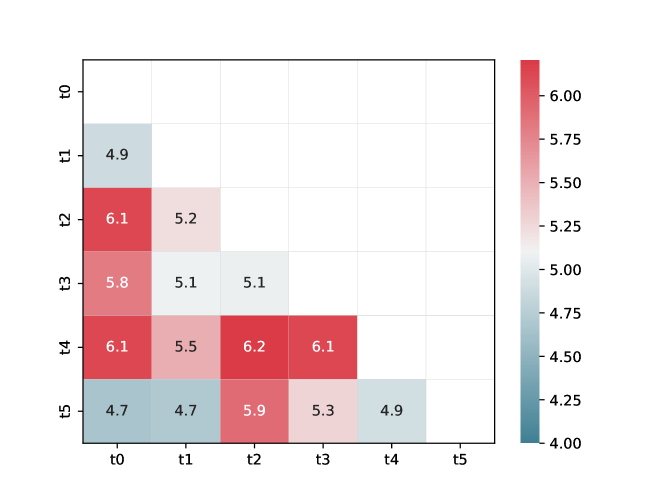
Figure 5: Task distances of each two topics in Topic-MSMARCO.

Table 1: Metadata and representative query terms of Topic-MSMARCO.

Topic index	Number of queries	Theme	Representative query terms
t0	64,719	IT	upload, emails, gmail, ios, icloud, cisco, photo, powerpoint, audio, instagram
t1	40,501	furnishing	doors, fiberglass, cement, drywall, fireplace, siding, stair, dryer, porch, ceramic
t2	51,002	food	broccoli, cabbage, canned, hamburger, fried, carrots, greens, peas, dried, tuna,
t3	47,646	health	painful, sleeping, vomiting, ache, weak, coughing, canine, uterus, lip, dysfunction, thrush, chronic, osteoarthritis, cell, mitochondria, subcutaneous, narrow, forehead,
t4	12,204	tourism	tampa, nashville, philadelphia, mall, downtown, rio, denver, veniceniagara, cape, hills metro, zoo, city, yellowstone
t5	46,326	finance	employers, qualified, orders, settlement, fraud, resident, reimbursement, charges, pays, residency, commission, officers

5.2 Experiment setup

The hardware environment for the experiments was an Nvidia RTX 3080 GPU workstation with an Intel 10700k CPU and 64GB of RAM. All neural network models in CLNIR were implemented using PyTorch. The word embedding vectors used were GloVe [48], and 300-dimensional word vectors were used as the initial weight for the embedding layer of DRMM, KNRM, and DUET. The PLM used for ColBERT and BERTdot is described in Wolf et al. [49].

5.3 Evaluating CLNIR using the topic-MSMARCO dataset

The first experiment aims to compare the continual learning performance of various combinations of neural retrieval models and learning strategies within the proposed CLNIR framework described in Section 4.

To eliminate the potential impact of inconsistent sample sizes in each task, $10\,000$ queries were randomly selected as the training set and $2\,000$ queries were selected as the test set for each task of Topic-MSMARCO. The CLNIR framework was used to pair neural ranking models with learning strategies, resulting in 35 continual retrieval methods. Five fine-tuning methods (without a learning strategy) were considered as baselines, bringing the total number of sub-experiments to 40.

5.3.1 Average final performance on topic-MSMarco using CLNIR

Table 2: Final performance scores for each task in topic-MSMARO and the final average performance.

		$P_{T,0}$	$P_{T,1}$	$P_{T,2}$	$P_{T,3}$	$P_{T,4}$	$P_{T,5}$	$P_{\mathrm{final}}$
DRMM	baseline	0.085	0.079	0.087	0.062	0.065	0.058	0.073±0.013
	L2	0.098	0.091	0.102	0.071	0.077	0.067	0.084±0.015
	EWC	0.101	0.088	0.099	0.061	0.072	0.067	0.081±0.017
	EWCol	0.105	0.093	0.095	0.068	0.074	0.068	0.084±0.016
	SI	0.101	0.086	0.098	0.058	0.070	0.063	0.079±0.018
	MAS	0.093	0.081	0.095	0.068	0.070	0.062	0.078±0.014
	NR	0.099	0.091	0.094	0.067	0.069	0.060	0.080±0.017
	GEM	0.070	0.065	0.069	0.052	0.054	0.046	0.059±0.010
KNRM	baseline	0.210	0.184	0.211	0.155	0.147	0.135	0.174±0.033
	L2	0.231	0.196	0.224	0.165	0.162	0.137	0.186±0.037
	EWC	0.231	0.195	0.224	0.165	0.161	0.136	0.185±0.038
	EWCol	0.231	0.195	0.224	0.164	0.161	0.136	0.185±0.038
	SI	0.230	0.196	0.224	0.164	0.161	0.137	0.185±0.038
	MAS	0.227	0.194	0.222	0.162	0.159	0.136	0.183±0.037
	NR	0.212	0.184	0.213	0.154	0.151	0.133	0.174±0.034
	GEM	0.156	0.139	0.17	0.113	0.122	0.122	0.137±0.022
DUET	baseline	0.148	0.134	0.125	0.095	0.134	0.133	0.128±0.018
	L2	0.169	0.157	0.145	0.119	0.137	0.152	0.147±0.017
	EWC	0.277	0.230	0.238	0.188	0.195	0.205	0.222±0.036
	EWCol	0.279	0.230	0.235	0.188	0.199	0.204	0.223±0.036
	SI	0.283	0.230	0.241	0.187	0.201	0.200	0.223±0.035
	MAS	0.215	0.189	0.191	0.151	0.161	0.178	0.181±0.023
	NR	0.236	0.186	0.196	0.165	0.167	0.166	0.186±0.027
	GEM	0.181	0.147	0.151	0.104	0.132	0.145	0.143±0.025
BERTdot	baseline	0.301	0.221	0.246	0.194	0.227	0.242	0.239±0.036
	L2	0.305	0.226	0.251	0.199	0.228	0.238	0.241±0.036
	EWC	0.318	0.215	0.237	0.177	0.207	0.216	0.228±0.048
	EWCol	0.255	0.202	0.219	0.177	0.200	0.214	0.211±0.026
	SI	0.320	0.215	0.238	0.180	0.209	0.217	0.23±0.048
	MAS	0.340	0.231	0.242	0.202	0.230	0.232	0.246±0.048
	NR	0.347	0.254	0.278	0.221	0.247	0.254	0.267±0.043
	GEM	0.314	0.223	0.252	0.197	0.228	0.246	0.243±0.040
ColBERT	baseline	0.402	0.336	0.335	0.273	0.307	0.302	0.326±0.044
	L2	0.421	0.344	0.334	0.285	0.320	0.302	0.334±0.048
	EWC	0.404	0.295	0.310	0.255	0.275	0.278	0.303±0.053
	EWCol	0.398	0.292	0.304	0.249	0.282	0.264	0.298±0.053
	SI	0.406	0.294	0.310	0.254	0.275	0.276	0.302±0.054
	MAS	0.411	0.328	0.337	0.286	0.309	0.304	0.329±0.044
	NR	0.431	0.350	0.361	0.299	0.330	0.324	0.349±0.045
	GEM	0.396	0.308	0.330	0.262	0.302	0.295	0.316±0.045

• The ‘baseline’ refers to the results of NIR models without a learning strategy; $P_{\mathrm{final}}$ represents the average final performance, while $P_{T,i}$ represents the final performance of the $i$th task in topic-MSMARCO.

Experiment description. The purpose of this experiment is to evaluate the performance of all pair combinations within the CLNIR framework using the Topic-MSMARCO dataset. The task sequence is organized from t0 to t5. The experiment results are presented in Table 2 and include the $P_{\mathrm{final}}$ scores for each pair combination and the overall performance scores for all tasks.

To determine the reliability of the Mean Reciprocal Rank (MRR) scores presented in Table 2, this study employs standard error tests. Specifically, for each MRR score, all the reciprocal ranks obtained from the corresponding test set are considered as the total samples. In each iteration, 400 samples are randomly selected, and their respective mean values are recorded. This random sampling process is repeated 100 times, resulting in 100 mean values. Finally, the standard error is computed as the standard deviation of these 100 mean values. As indicated in Table 2, the computed standard errors for all MRR scores are approximately 0.01 and 0.02, respectively. These values suggest that the obtained results are reliable and not merely random fluctuations.

DRMM group. As seen in the second row of Table 2, except for its combinations with EWC, EWCol, and SI at t0, all other final performance scores are lower than 0.1, representing the worst performance among all NIR groups. Despite the low MRR scores, some continual learning strategies led to performance improvement. Without the use of any learning strategy, the average score is 0.073. On the other hand, the average score improves to 0.084 when using the L2 or EWCol strategy. The EWC, MAS, NR, and SI strategies also had a positive effect on the final performance. However, the GEM strategy did not offer any performance improvement in the DRMM group, leading to a lower average MRR score compared to the baseline.

KNRM group. As indicated in the third row of Table 2, the baseline MRR score is 0.174. The L2, EWC, EWCol, SI, and MAS strategies resulted in higher scores, ranging from 0.183 to 0.186, with the highest score achieved by the L2 strategy. The NR strategy performed similarly to the baseline. The only strategy that negatively impacted the average final performance was GEM, with a score of 0.143, which was 0.031 lower than the baseline.

DUET group. As shown in the fourth row of Table 2, continual learning strategies showed the greatest improvement in the DUET group, as it is the only group where all pair combinations of NIR model with various learning strategies outperformed the baseline method. In particular, the average final performance of EWC and SI was 0.223 in the DUET group, representing an increase of 0.095 compared to the baseline, which was also the largest improvement among all NIR groups. The average final performance score for the baseline was 0.128. The average final performance for the L2 and GEM strategies reached 0.14, while the average final performance for EWCol, MAS, and NR strategies reached 0.18.

BERTdot group. As seen in the fifth row of Table 2, all average final performance scores are above 0.2. The baseline score is 0.239, and both replay strategies (NR, GEM) outperformed the baseline method. The highest score in this group was achieved by NR, with a score of 0.267, which was 0.028 higher than the baseline. It is worth noting that among all the regularization-based strategies, only MAS and L2 had a slight improvement over the baseline score, while the two EWC strategies actually resulted in lower scores compared to the baseline.

ColBERT group. ColBERT outperformed the other models in this experiment. All strategies except for EWCol resulted in an average final performance score higher than 0.3. Similar to the BERTdot group, NR achieved the highest score of 0.349. Both EWC strategies and GEM had an inferior performance compared to the baseline, while L2 and MAS slightly improved the baseline by 0.008 and 0.003, respectively.

5.3.2 The BWT performance on topic-MSMarco using CLNIR

This experiment is to compare the BWT and FWT performance of each pair combination in CLNIR.

BWT performance of baseline methods. As demonstrated in Table 3, all the baseline methods experienced catastrophic forgetting as all their BWT scores are negative. The BWT scores of the DUET and BERTdot models are a few hundredths below zero, indicating that they are more susceptible to forgetting without learning strategies, compared to the remaining NIR models whose BWT scores are a few thousandths under zero.

Impact of learning strategies on BWT. As shown in Table 3, when combined with learning strategies, all models, except for KNRM, achieved BWT scores higher than zero, indicating that NIR models can perform better on BWT with learning strategies. Although the KNRM group did not produce any positive BWT scores, the highest score was negative by only several millionths, indicating a significant reduction in catastrophic forgetting. The DUET model achieved the highest BWT scores with the EWC and SI strategies, at 1.65e-2 and 1.6e-2 respectively. ColBERT showed a higher degree of adaptability to diverse learning strategies, with four of its BWT scores greater than zero.

Learning strategies comparison on BWT. With regards to the learning strategies, according to Table 3, the SI strategy was observed to achieve the most positive BWT scores, outperforming the other strategies. Both the MAS and NR strategies had two positive BWT scores on two pretraining-based models. Meanwhile, the L2 and two EWC strategies generated one positive score. The GEM strategy was the only one that was unable to overcome catastrophic forgetting.

Table 3: Backward transfer performance of CLNIR.

	DRMM	KNRM	DUET	BERTdot	ColBERT
baseline	-9.10E-03	-7.29E-03	-3.73E-02	-1.25E-02	-2.42E-03
L2	-3.06E-03	-3.93E-05	-2.07E-02	-1.04E-02	3.60E-03
EWC	-4.92E-04	-7.25E-06	1.65E-02	-3.56E-04	-1.72E-04
EWCol	2.00E-04	-5.25E-05	1.87E-02	-1.38E-02	-5.91E-05
SI	2.49E-04	-2.12E-04	1.66E-02	4.68E-04	6.40E-04
MAS	-7.14E-03	-1.93E-03	-6.26E-03	1.22E-03	2.95E-03
NR	-4.23E-03	-6.70E-03	-4.04E-03	8.10E-03	7.75E-03
GEM	-1.29E-02	-2.85E-02	-3.23E-02	-9.50E-03	-6.55E-03

5.3.3 FWT performance on topic-MSMarco using CLNIR

Impact of learning strategies on NIR models. Table 4 indicates that the FWT scores of the NIR groups that pretraining-based NIR models outperformed the embedding-based ones, consistent with their average final performance. ColBERT paired with the NR strategy achieved the highest FWT score (0.303). The combination of BERTdot and NR also achieved the best performance in the BERTdot group. In the DUET group, the EWCol strategy produced the best result with a score of 0.166, followed closely by EWC and SI with scores of 0.165. In the KNRM group, four regularization learning strategies (L2, EWC, EWCol, SI) tied for the highest FWT score. In the DRMM group, L2 and NR ranked first with a score of 0.072.

Comparing FWT between baselines and learning strategies. Table 4 reveals that all learning strategies except for the GEM strategy increased the baseline FWT scores to varying degrees in both the DRMM and KNRM groups. All strategies resulted in higher FWT scores compared to the baseline model in the DUET group. In the two groups with pertaining NIR models, it is noteworthy that several learning strategies had a negative impact on FWT performance. Specifically, three strategies (L2, EWC,SI) produced lower FWT scores compared to the baseline in the BERTdot group, while the NR strategy was the only one that outperformed the baseline method in the ColBERT group.

Table 4: Forward transfer performance of CLNIR.

	DRMM	KNRM	DUET	BERTdot	ColBERT
baseline	0.069	0.160	0.142	0.219	0.295
L2	0.072	0.164	0.146	0.218	0.292
EWC	0.071	0.164	0.165	0.208	0.277
EWCol	0.073	0.164	0.166	0.224	0.273
SI	0.069	0.164	0.165	0.208	0.277
MAS	0.071	0.161	0.154	0.225	0.292
NR	0.072	0.160	0.153	0.228	0.303
GEM	0.061	0.156	0.151	0.220	0.289

• All standard error scores are less than 0.03.

5.3.4 Overall comparison

Best learning strategy. From the previous comparisons of the final average performance, BWT and FWT, it can be observed that all five NIR models benefit from learning strategies. NIR models combined with the appropriate learning strategies always outperform the baseline methods in any evaluation metric. It is also noteworthy that the two pretraining NIR models experienced the greatest improvement when combined with the NR strategy, as all three metrics are the best in their respective groups. However, the optimal learning strategies for different embedding-based NIR models vary. The best learning strategies for different NIR models and evaluation metrics are listed in detail in Table 5.

Table 5: Best learning strategies for different NIR models and different evaluation metrics.

	$P_{\mathrm{final}}$	BWT	FWT
DRMM	L2	SI	L2/NR
KNRM	L2	EWC	L2/EWC/EWCol/SI
DUET	SI	EWCol	EWCol
BERTdot	NR	NR	NR
ColBERT	NR	NR	NR

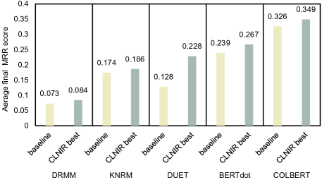
(a) Average final MRR

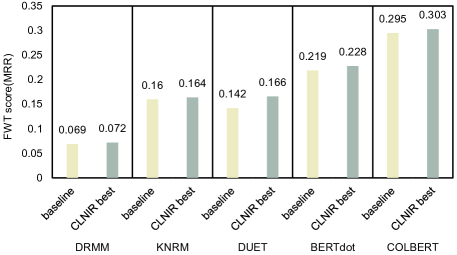
(b) Forward transfer ability

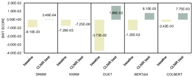
(c) Backward transfer ability

Figure 6: Performance comparison between baseline and CLNIR best.

To provide further insight into the effectiveness of learning strategies, the performance scores of three metrics on the five NIR models are depicted in Figure 6. For ease of comparison, the combination of NIR models and their best corresponding learning strategies will be referred to as “CLNIR best”.

5.4 Evaluating the impact of data volume and topic shift on continual NIR

This subsection will evaluate the impact of topic shift and data volume on continual information retrieval.

5.4.1 Impact of topic shift distance on continual learning performance

Aim and methodology of the experiment. The aim of the experiment is to explore the impact of topic shift distances on the performance of NIR tasks in continual learning. The methodology is as follows:

• Topic t1 (“furnishing”) was selected as the starting point because it had the smallest mean standard deviation among the other topics, resulting in the most uniform topic distances according to Figure 5.

• The remaining topics (t0, t2-t5) were learned in parallel as the second topics. Therefore, five sub-experiments were conducted, each with two topics.

• The NIR models used for the experiment were KNRM and ColBERT, as their baseline methods performed the best among embedding-based and pretraining-based models, respectively.

• The continual learning strategy used was the SI strategy, as it achieved the most positive FWT scores (4 in total) in Table 3.

Analysing the topic shift in the KNRM group. According to Figure 7(a), the baseline KNRM model without a learning strategy shows that as the topic distance increases, the MRR score decreases. The Pearson correlation coefficient between topic distances and MRR scores is -0.953. However, when combined with the SI strategy, the decrease in performance is less severe because the performance curve of the SI strategy has a slower decline rate compared to the baseline. This implies that the SI strategy can effectively mitigate the issue of catastrophic forgetting while learning a new task, especially when the topic distance is greater than 4.9. In such cases, the MRR scores generated with the SI strategy are both more stable and higher than those of the baseline methods.

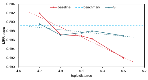
(a) Topic shift phenomenon of KNRM model

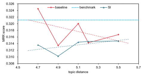
(b) Topic shift phenomenon of ColBERT model

Figure 7: Impact of topic shift on continual learning performance. The “benchmark” refers to the results obtained prior to learning the second task; the “baseline” represents the results of NIR models without implementing any learning strategies; and “SI” refers to the results of models that have been combined with SI strategy.

Analysing the topic shift in the ColBERT group. Figure 7(b) demonstrates that ColBERT produced different results compared to the KNRM group. The MRR performance curve for the baseline ColBERT displays fluctuations as the topic distance increases, resulting in a general decline in MRR scores. On the other hand, the MRR curve for the ColBERT combined with SI shows a narrower range of fluctuation, however, the MRR scores are lower than those of the baseline ColBERT. This suggests that ColBERT does not consistently show a decrease in MRR scores with increasing topic distance. Furthermore, when combined with the SI strategy, the majority of the MRR scores are lower than the baseline.

5.4.2 Impact of data volume on continual learning performance

Aim and methodology of the experiment. The aim of this experiment is to investigate the relationship between data volume and performance. The methodology for conducting this experiment is described below:

• KNRM and ColBERT were chosen as the tested NIR models and the SI strategy was employed. The reasons for these choices are as previously stated.

• The initial task was selected to be “tourism” (t4) and the subsequent task was “food” (t2), as these two topics were deemed to have the greatest disparity among all topic pairs.

• The influence of varying training sample sizes on model performance was assessed by setting the sample size for the second task in a flexible manner. Considering that the sample size for task 2 is approximately five times larger than that of task 1, the sample size for task 2 was established to range from 0.1 to 1 times, incrementing by 0.1 at each interval, and then from 1 to 5 times with an interval of 1.

Analysing the data volume in the KNRM group. The relationship between data volume and the performance of KNRM methods is demonstrated in Figure 8(a). It has been observed that in the baseline KNRM method, there exists a negative correlation between data volume and continual learning performance, where the data volume of the new task is one time larger. This correlation is measured using the Pearson correlation coefficient of -0.987. On the other hand, the SI-combined KNRM method exhibits more stable results, indicating that the SI strategy effectively reduces the impact of data volume. It should be noted that both KNRM methods exhibit an upward trend when the sample size of the subsequent task is smaller than the initial task, which suggests that embedding-based models can still benefit from small-scale new tasks even when there is a significant topic distance.

Analysing the data volume in the ColBERT group. The results for the ColBERT group are depicted in Figure 8(b). It is shown that the SI-combined ColBERT method provides more stable performance compared to the baseline ColBERT method, but it failed to achieve higher scores. Both methods have local high points when the sample size of the subsequent task is one time smaller, which is similar to the findings in the KNRM group. However, the baseline ColBERT method demonstrates a weaker correlation with data volume, with a Pearson correlation coefficient of 0.490. This is further evidenced by the fluctuating performance curve.

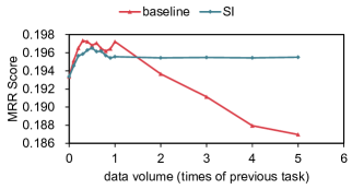
(a) Results of the KNRM group.

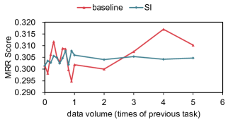
(b) Results of the ColBERT group.

Figure 8: Impact of data volume on continual learning performance.

5.5 Key findings

Three experiments were conducted to evaluate the performance of the proposed CLNIR framework and reveal the relationships between continual learning performance, topic shift, and data volume.

Findings about the continual learning performance of CLNIR. The findings of the first experiment showed that pretraining-based NIR models outperformed embedding-based models in terms of average final performance and forward transfer performance. The forward transfer performance rank order was similar to that of the final average performance. For pretraining-based NIR models, the NR strategy was found to be the most effective, while the best strategy for embedding-based NIR models varied. However, in some instances, the GEM-combined NIR models performed worse than the baseline approaches. These results demonstrate the effectiveness of the proposed CLNIR framework in mitigating the catastrophic forgetting phenomenon and improving continual learning performance in NIR tasks.

Findings about topic shift and data augmentation. In the second and third experiments, it was observed that both topic shift distance and data augmentation have a negative correlation with continual learning performance when using the embedding-based baseline method. As the topic shift distance or data volume increases, the continual learning performance tends to decrease. However, the use of a learning strategy such as SI can mitigate this trend. This pattern is also evident in the pretraining-based baseline methods, where MRR curves fluctuate with the increment of topic shift distance or data volume, but models combined with SI are consistently more stable than those baseline models. While learning strategies can address the issue of catastrophic forgetting caused by topic shifts or data augmentation, they may also diminish the performance improvements caused by a new task.

6 Conclusion

This paper presents a task formulation and novel dataset for continual neural information retrieval tasks and introduces a framework called CLNIR for addressing the lack of continual learning ability in current NIR models. The CLNIR includes several typical NIR models and learning strategies. Experiments were conducted to evaluate the performance of different pair combinations of NIR models and learning strategies in the framework. The results show that the best learning strategies for different NIR models vary, but NIR models combined with a suitable learning strategy can always outperform the baseline methods where no learning strategy is used. Additionally, the impact of topic shift and data augmentation has also been investigated through experiments. It has been found that learning strategies can mitigate the impact of topic shift and data augmentation, leading to more stable performance. In conclusion, the proposed CLNIR framework can effectively deal with the catastrophic forgetting problem in real-world information retrieval systems and applications. The proposed framework can even improve the performance of old data by learning new data.

The limitations of the study are that only a limited number of NIR models and learning strategies were included in the CLNIR framework, and the dataset consists only of question-answer pairs. Future work will include incorporating additional NIR modules and novel learning strategies; and the application of the CLNIR framework to other information retrieval paradigms, such as document ranking and recommender systems.

Data availability

The data described in this paper was obtained from the public repository available at https://microsoft.github.io/msmarco/. To reorganize the dataset and reproduce the experiments, please refer to the paper’s GitHub repository located at https://github.com/[whitespace].

References

- Ceri et al. [2013] S. Ceri, A. Bozzon, M. Brambilla, E. Della Valle, P. Fraternali, S. Quarteroni, An Introduction to Information Retrieval, Springer Berlin Heidelberg, Berlin, Heidelberg, 2013, pp. 3–11. doi:10.1007/978-3-642-39314-3_1.
- guo [2020] A deep look into neural ranking models for information retrieval, Inf. Process. Manage. 57 (2020) 102067. doi:10.1016/j.ipm.2019.102067.
- Huang et al. [2013] P.-S. Huang, X. He, J. Gao, L. Deng, A. Acero, L. Heck, Learning deep structured semantic models for web search using clickthrough data, in: Proceedings of the 22nd ACM International Conference on Information & Knowledge Management, CIKM ’13, Association for Computing Machinery, New York, NY, USA, 2013, p. 2333–2338. doi:10.1145/2505515.2505665.
- Guo et al. [2016] J. Guo, Y. Fan, Q. Ai, W. B. Croft, A deep relevance matching model for Ad-Hoc retrieval, in: Proceedings of the 25th ACM International on Conference on Information and Knowledge Management, CIKM ’16, Association for Computing Machinery, New York, NY, USA, 2016, p. 55–64. doi:10.1145/2983323.2983769.
- Xiong et al. [2017] C. Xiong, Z. Dai, J. Callan, Z. Liu, R. Power, End-to-end neural Ad-Hoc ranking with kernel pooling, in: Proceedings of the 40th International ACM SIGIR Conference on Research and Development in Information Retrieval, SIGIR ’17, Association for Computing Machinery, New York, NY, USA, 2017, p. 55–64. doi:10.1145/3077136.3080809.
- Mitra et al. [2017] B. Mitra, F. Diaz, N. Craswell, Learning to match using local and distributed representations of text for web search, in: Proceedings of the 26th International Conference on World Wide Web, WWW ’17, International World Wide Web Conferences Steering Committee, Republic and Canton of Geneva, CHE, 2017, p. 1291–1299. doi:10.1145/3038912.3052579.
- Passalis and Tefas [2018] N. Passalis, A. Tefas, Learning bag-of-embedded-words representations for textual information retrieval, Pattern Recognit. 81 (2018) 254–267. doi:10.1016/j.patcog.2018.04.008.
- MacAvaney et al. [2019a] S. MacAvaney, A. Yates, A. Cohan, N. Goharian, CEDR: Contextualized embeddings for document ranking, in: Proceedings of the 42nd International ACM SIGIR Conference on Research and Development in Information Retrieval, 2019a, pp. 1101–1104.
- MacAvaney et al. [2019b] S. MacAvaney, A. Yates, A. Cohan, N. Goharian, CEDR: Contextualized embeddings for document ranking, in: Proceedings of the 42nd International ACM SIGIR Conference on Research and Development in Information Retrieval, SIGIR’19, Association for Computing Machinery, New York, NY, USA, 2019b, p. 1101–1104. doi:10.1145/3331184.3331317.
- Devlin et al. [2019] J. Devlin, M. Chang, K. Lee, K. Toutanova, BERT: pre-training of deep bidirectional transformers for language understanding, in: J. Burstein, C. Doran, T. Solorio (Eds.), Proceedings of the 2019 Conference of the North American Chapter of the Association for Computational Linguistics: Human Language Technologies, NAACL-HLT 2019, Minneapolis, MN, USA, June 2-7, 2019, Volume 1 (Long and Short Papers), Association for Computational Linguistics, 2019, pp. 4171–4186. doi:10.18653/v1/n19-1423.
- Chen and Liu [2018] Z. Chen, B. Liu, Related Learning Paradigms, Springer International Publishing, Cham, 2018, pp. 21–34. doi:10.1007/978-3-031-01581-6_2.
- Han et al. [2021] Y. Han, S. Karunasekera, C. Leckie, Continual learning for fake news detection from social media, in: International Conference on Artificial Neural Networks, Springer, 2021, pp. 372–384.
- Harun et al. [2023] M. Y. Harun, J. Gallardo, T. L. Hayes, C. Kanan, How efficient are today’s continual learning algorithms?, in: Proceedings of the IEEE/CVF Conference on Computer Vision and Pattern Recognition, 2023, pp. 2430–2435.
- Pratama and Wang [2019] M. Pratama, D. Wang, Deep stacked stochastic configuration networks for lifelong learning of non-stationary data streams, Inf. Sci. 495 (2019) 150–174. doi:10.1016/j.ins.2019.04.055.
- Biesialska et al. [2020] M. Biesialska, K. Biesialska, M. R. Costa-jussà, Continual lifelong learning in natural language processing: A survey, in: Proceedings of the 28th International Conference on Computational Linguistics, International Committee on Computational Linguistics, Barcelona, Spain (Online), 2020, pp. 6523–6541. doi:10.18653/v1/2020.coling-main.574.
- McCloskey and Cohen [1989] M. McCloskey, N. J. Cohen, Catastrophic interference in connectionist networks: The sequential learning problem, volume 24 of Psychology of Learning and Motivation, Academic Press, 1989, pp. 109–165. doi:10.1016/S0079-7421(08)60536-8.
- French [1999] R. M. French, Catastrophic forgetting in connectionist networks, TRENDS COGN. SCI. 3 (1999) 128–135. doi:10.1016/S1364-6613(99)01294-2.
- Lange et al. [2022] M. D. Lange, R. Aljundi, M. Masana, S. Parisot, X. Jia, A. Leonardis, G. G. Slabaugh, T. Tuytelaars, A continual learning survey: Defying forgetting in classification tasks, IEEE Trans. Pattern Anal. Mach. Intell. 44 (2022) 3366–3385. doi:10.1109/TPAMI.2021.3057446.
- Mai et al. [2022] Z. Mai, R. Li, J. Jeong, D. Quispe, H. Kim, S. Sanner, Online continual learning in image classification: An empirical survey, Neurocomputing 469 (2022) 28–51. doi:10.1016/j.neucom.2021.10.021.
- Lovón-Melgarejo et al. [2021] J. Lovón-Melgarejo, L. Soulier, K. Pinel-Sauvagnat, L. Tamine, Studying catastrophic forgetting in neural ranking models, in: D. Hiemstra, M.-F. Moens, J. Mothe, R. Perego, M. Potthast, F. Sebastiani (Eds.), Advances in Information Retrieval, Springer International Publishing, Cham, 2021, pp. 375–390. doi:10.1007/978-3-030-72113-8_25.
- Gerald and Soulier [2022] T. Gerald, L. Soulier, Continual learning of long topic sequences in neural information retrieval, in: European Conference on Information Retrieval, Springer, 2022, pp. 244–259. doi:10.1007/978-3-030-99736-6_17.
- Perkonigg et al. [2021] M. Perkonigg, J. Hofmanninger, C. J. Herold, J. A. Brink, O. Pianykh, H. Prosch, G. Langs, Dynamic memory to alleviate catastrophic forgetting in continual learning with medical imaging, Nat. Commun. 12 (2021) 1–12. doi:10.1038/s41467-021-25858-z.
- Shi et al. [2021] G. Shi, J. Chen, W. Zhang, L.-M. Zhan, X.-M. Wu, Overcoming catastrophic forgetting in incremental few-shot learning by finding flat minima, Adv. Neural. Inf. Process. Syst. 34 (2021) 6747–6761. doi:10.48550/arXiv.2111.01549.
- Wei and Li [2022] G. Wei, X. Li, Knowledge lock: Overcoming catastrophic forgetting in federated learning, Springer-Verlag, Berlin, Heidelberg, 2022, p. 601–612. doi:10.1007/978-3-031-05933-9_47.
- Doan et al. [2021] T. Doan, M. Abbana Bennani, B. Mazoure, G. Rabusseau, P. Alquier, A theoretical analysis of catastrophic forgetting through the NTK overlap matrix, in: A. Banerjee, K. Fukumizu (Eds.), Proceedings of The 24th International Conference on Artificial Intelligence and Statistics, volume 130 of Proceedings of Machine Learning Research, PMLR, 2021, pp. 1072–1080.
- Lee et al. [2021] S. Lee, S. Goldt, A. Saxe, Continual learning in the teacher-student setup: Impact of task similarity, in: M. Meila, T. Zhang (Eds.), Proceedings of the 38th International Conference on Machine Learning, volume 139 of Proceedings of Machine Learning Research, PMLR, 2021, pp. 6109–6119.
- Evron et al. [2022] I. Evron, E. Moroshko, R. Ward, N. Srebro, D. Soudry, How catastrophic can catastrophic forgetting be in linear regression?, in: P.-L. Loh, M. Raginsky (Eds.), Proceedings of Thirty Fifth Conference on Learning Theory, volume 178 of Proceedings of Machine Learning Research, PMLR, 2022, pp. 4028–4079.
- Kirkpatrick et al. [2017] J. Kirkpatrick, R. Pascanu, N. Rabinowitz, J. Veness, G. Desjardins, A. A. Rusu, K. Milan, J. Quan, T. Ramalho, A. Grabska-Barwinska, D. Hassabis, C. Clopath, D. Kumaran, R. Hadsell, Overcoming catastrophic forgetting in neural networks, Proc. Natl. Acad. Sci. U. S. A. 114 (2017) 3521–3526. doi:10.1073/pnas.1611835114.
- Zenke et al. [2017] F. Zenke, B. Poole, S. Ganguli, Continual learning through synaptic intelligence, in: Proceedings of the 34th International Conference on Machine Learning - Volume 70, ICML’17, JMLR.org, 2017, p. 3987–3995.
- Aljundi et al. [2018] R. Aljundi, F. Babiloni, M. Elhoseiny, M. Rohrbach, T. Tuytelaars, Memory aware synapses: Learning what (not) to forget, in: V. Ferrari, M. Hebert, C. Sminchisescu, Y. Weiss (Eds.), Computer Vision – ECCV 2018, Springer International Publishing, Cham, 2018, pp. 144–161. doi:10.1007/978-3-030-01219-9_9.
- Mazur et al. [2022] M. Mazur, Ł. Pustelnik, S. Knop, P. Pagacz, P. Spurek, Target layer regularization for continual learning using cramer-wold distance, Inf. Sci. 609 (2022) 1369–1380. doi:10.1016/j.ins.2022.07.085.
- Zhang et al. [2023] L. Zhang, S. Wang, F. Yuan, B. Geng, M. Yang, Lifelong language learning with adaptive uncertainty regularization, Inf. Sci. 622 (2023) 794–807. doi:10.1016/j.ins.2022.11.141.
- Rebuffi et al. [2017] S.-A. Rebuffi, A. Kolesnikov, G. Sperl, C. H. Lampert, iCaRL: Incremental classifier and representation learning, in: Proceedings of the IEEE Conference on Computer Vision and Pattern Recognition, 2017, pp. 2001–2010. doi:10.1109/CVPR.2017.587.
- Lopez-Paz and Ranzato [2017] D. Lopez-Paz, M. Ranzato, Gradient episodic memory for continual learning, in: Proceedings of the 31st International Conference on Neural Information Processing Systems, NIPS’17, Curran Associates Inc., Red Hook, NY, USA, 2017, p. 6470–6479.
- Zhuang et al. [2022] C. Zhuang, S. Huang, G. Cheng, J. Ning, Multi-criteria selection of rehearsal samples for continual learning, Pattern Recognit. 132 (2022) 108907. doi:10.1016/j.patcog.2022.108907.
- Rusu et al. [2016] A. A. Rusu, N. C. Rabinowitz, G. Desjardins, H. Soyer, J. Kirkpatrick, K. Kavukcuoglu, R. Pascanu, R. Hadsell, Progressive neural networks, CoRR abs/1606.04671 (2016). arXiv:1606.04671.
- Aljundi et al. [2017] R. Aljundi, P. Chakravarty, T. Tuytelaars, Expert gate: Lifelong learning with a network of experts, in: 2017 IEEE Conference on Computer Vision and Pattern Recognition, CVPR 2017, Honolulu, HI, USA, July 21-26, 2017, IEEE Computer Society, 2017, pp. 7120–7129. doi:10.1109/CVPR.2017.753.
- Wang et al. [2021] K. Wang, L. Herranz, J. van de Weijer, Continual learning in cross-modal retrieval, in: IEEE Conference on Computer Vision and Pattern Recognition Workshops, CVPR Workshops 2021, virtual, June 19-25, 2021, Computer Vision Foundation / IEEE, 2021, pp. 3628–3638. doi:10.1109/CVPRW53098.2021.00402.
- Song et al. [2023] G. Song, X. Tan, M. Yang, Deep continual hashing with gradient-aware memory for cross-modal retrieval, Pattern Recognit. 137 (2023) 109276. doi:10.1016/j.patcog.2022.109276.
- Nguyen et al. [2016] T. Nguyen, M. Rosenberg, X. Song, J. Gao, S. Tiwary, R. Majumder, L. Deng, MS MARCO: A human generated machine reading comprehension dataset, in: T. R. Besold, A. Bordes, A. S. d’Avila Garcez, G. Wayne (Eds.), Proceedings of the Workshop on Cognitive Computation: Integrating neural and symbolic approaches 2016 co-located with the 30th Annual Conference on Neural Information Processing Systems (NIPS 2016), Barcelona, Spain, December 9, 2016, volume 1773 of CEUR Workshop Proceedings, CEUR-WS.org, 2016.
- Nogueira and Cho [2019] R. F. Nogueira, K. Cho, Passage re-ranking with BERT, CoRR abs/1901.04085 (2019). arXiv:1901.04085.
- Harman [2011] D. Harman, Interactive Evaluation, Springer International Publishing, Cham, 2011, pp. 57–75. doi:10.1007/978-3-031-02276-0_3.
- Amigó et al. [2018] E. Amigó, D. Spina, J. Carrillo-de Albornoz, An axiomatic analysis of diversity evaluation metrics: Introducing the rank-biased utility metric, in: The 41st International ACM SIGIR Conference on Research & Development in Information Retrieval, SIGIR ’18, Association for Computing Machinery, New York, NY, USA, 2018, p. 625–634. doi:10.1145/3209978.3210024.
- Rodríguez et al. [2018] N. D. Rodríguez, V. Lomonaco, D. Filliat, D. Maltoni, Don’t forget, there is more than forgetting: new metrics for continual learning, CoRR abs/1810.13166 (2018). arXiv:1810.13166.
- Hsu et al. [2018] Y. Hsu, Y. Liu, Z. Kira, Re-evaluating continual learning scenarios: A categorization and case for strong baselines, CoRR abs/1810.12488 (2018). arXiv:1810.12488.
- Hofstätter et al. [2021] S. Hofstätter, S.-C. Lin, J.-H. Yang, J. Lin, A. Hanbury, Efficiently teaching an effective dense retriever with balanced topic aware sampling, in: Proceedings of the 44th International ACM SIGIR Conference on Research and Development in Information Retrieval, SIGIR ’21, Association for Computing Machinery, New York, NY, USA, 2021, p. 113–122. doi:10.1145/3404835.3462891.
- Hong et al. [2021] Y. Hong, H. Xie, G. Bhumbra, I. Brilakis, Comparing natural language processing methods to cluster construction schedules, J. Constr. Eng. Manage. 147 (2021) 04021136. doi:10.1061/(ASCE)CO.1943-7862.0002165.
- Pennington et al. [2014] J. Pennington, R. Socher, C. Manning, GloVe: Global vectors for word representation, in: Proceedings of the 2014 Conference on Empirical Methods in Natural Language Processing (EMNLP), Association for Computational Linguistics, Doha, Qatar, 2014, pp. 1532–1543. doi:10.3115/v1/D14-1162.
- Wolf et al. [2020] T. Wolf, L. Debut, V. Sanh, J. Chaumond, C. Delangue, A. Moi, P. Cistac, T. Rault, R. Louf, M. Funtowicz, J. Davison, S. Shleifer, P. von Platen, C. Ma, Y. Jernite, J. Plu, C. Xu, T. Le Scao, S. Gugger, M. Drame, Q. Lhoest, A. Rush, Transformers: State-of-the-art natural language processing, in: Proceedings of the 2020 Conference on Empirical Methods in Natural Language Processing: System Demonstrations, Association for Computational Linguistics, Online, 2020, pp. 38–45. doi:10.18653/v1/2020.emnlp-demos.6.