A new understanding of grazing limit

Abstract.

The grazing limit of the Boltzmann equation to Landau equation is well-known and has been justified by using cutoff near the grazing angle with some suitable scaling. In this paper, we will provide a new understanding by simply applying a natural scaling on the Boltzmann operator without angular cutoff. The proof is based on a new well-posedness theory on the Boltzmann equation without angular cutoff in the regime with optimal ranges of parameters so that the grazing limit can be justified directly for any $\gamma>-5$ that includes the Coulomb potential corresponding to $\gamma=-3$. With this new understanding, the scaled Boltzmann operator in fact can be decomposed into two components. The first one converges to the Landau operator when the singular parameter $s$ of interaction angle tends to $1^{-}$ and the second one vanishes in this limit.

AMS Subject Classification (2010): 35Q20, 35R11, 75P05.

1. Introduction

The Boltzmann and Landau equations are the two most classical kinetic equations. Regarding to the Cauchy problem, there has been extensive work in different frameworks, e.g. [29, 30, 5, 6, 10, 25, 31, 32, 16, 17, 18, 9, 26, 27, 28, 15, 2, 19, 22, 13]. In fact, the Landau equation was derived by Landau in 1936 from the Boltzmann equation with cutoff Rutherford cross section. Mathematical justification of the grazing collision limit has proved to be successful since 1990s by adding a cutoff angle with suitable scaling parameter to the Boltzmann cross-section, cf. [3, 4, 7, 8, 14, 20, 21, 23, 12].

This paper aims to provide a new approach to justisfy this limit so that the relation between the Boltzmann equation and Landau equation can be understood from a different angle. Precisely, we study the grazing limit directly starting from the Boltzmann equation with angular non-cutoff kernels $B^{s,\gamma}(v-v_{*},\sigma)\sim\theta^{-2-2s}|v-v_{*}|^{\gamma}$ originating from the inverse power law potentials. Roughly speaking, with a proper scaling to the Boltzmann cross-section, when parameter of the angular singularity $s\to 1^{-}$, we naturally justify the limit to the Landau equation for any $\gamma>-5$. We point out that this new approach is related to but very different from the existing arguments for grazing limit.

1.1. A natural scaling

Consider the Cauchy problem of the Landau equation

$$\left\{\begin{aligned} &\partial_{t}F+v\cdot\nabla_{x}F=Q_{L}^{\gamma}(F,F),~{}~{}t>0,x\in\mathbb{T}^{3},v\in\mathop{\mathbb{R}\kern 0.0pt}\nolimits^{3},\\ &F|_{t=0}=F_{0}.\end{aligned}\right.$$ (1.1)

Here the Landau operator $Q_{L}^{\gamma}(g,h)$ is defined by

$$Q_{L}^{\gamma}(g,h)(v):=\nabla_{v}\cdot\bigg{\{}\int_{\mathop{\mathbb{R}\kern 0.0pt}\nolimits^{3}}a^{\gamma}(v-v_{*})[g(v_{*})\nabla_{v}h(v)-\nabla_{v_{*}}g(v_{*})h(v)]\mathrm{d}v_{*}\bigg{\}}.$$ (1.2)

where the symmetric matrix $a^{\gamma}$ is given by

$$a^{\gamma}(z)=\Lambda|z|^{\gamma+2}\Pi(z),\quad\Pi(z):=(I_{3}-\frac{z\otimes z}{|z|^{2}}).$$ (1.3)

Here, $I_{3}$ is the $3\times 3$ identity matrix and $\Lambda$ is a constant.

We will show that the solution $F_{L}^{\gamma}$ of (1.1) can be derived from that of the Boltzmann equation with a natural scaling. Let $F^{s,\gamma}_{B}$ be the solution to the Boltzmann equation

$$\partial_{t}F+v\cdot\nabla_{x}F=Q^{s,\gamma}_{B}(F,F),\quad F|_{t=0}=(1-s)F_{0},$$ (1.4)

where $Q^{s,\gamma}_{B}$ is the Boltzmann operator defined by

$$Q^{s,\gamma}_{B}(g,h)(v):=\int_{\mathop{\mathbb{R}\kern 0.0pt}\nolimits^{3}}\int_{\mathbb{S}^{2}}B^{s,\gamma}(v-v_{*},\sigma)\left(g^{\prime}_{*}h^{\prime}-g_{*}h\right)\mathrm{d}\sigma\mathrm{d}v_{*}.$$ (1.5)

Here, $B^{s,\gamma}$ is the angular non-cutoff kernel derived from inverse power law potentials, given by

$$B^{s,\gamma}(v-v_{*},\sigma)=C_{s,\gamma}(\sin\frac{\theta}{2})^{-2-2s}|v-v_{*}|^{\gamma}.$$ (1.6)

The main result in this paper is to rigorously prove for $\gamma>-5$,

$$F^{s,\gamma}_{B}/(1-s)\to F_{L}^{\gamma},\quad s\to 1^{-}.$$ (1.7)

This can be stated mathematically as that the Boltzmann equation with a proper scaling tends to the Landau equation as $s\to 1^{-}$.

Recall that (1.6) is derived from the inverse power law potential $U(r)=r^{-p}$. For $p\geq 1$, one has $s=1/p,\gamma=1-4s$. The Coulomb potential corresponds to $p=s=1,\gamma=-3$. In order to treat the Coulomb potential physically, we can take $\gamma=1-4s$ and study the limit $s\to 1^{-}$. Our result directly yield limit to the Landau equation with $\gamma=-3$ in (1.7). To be more general in mathematics, in the following discussion, we will regard $\gamma$ as a fixed constant in the range $\gamma>-5$ for Landau and $\gamma>-3-2s$ for Boltzmann.

In the existing literatures on the grazing limit, for instance in [8], by introducing a cutoff $\theta\gtrsim\epsilon$ and by suitably adding the scaling factor $\epsilon^{2s-2}$, Desvillettes considered the scaled Boltzmann kernel $B^{\epsilon,s,\gamma}(v-v_{*},\sigma)=\epsilon^{2s-2}(\sin\frac{\theta}{2})^{-2-2s}\mathrm{1}_{0\leq\theta\leq\epsilon}|v-v_{*}|^{\gamma}$ and studied the limit $\epsilon\to 0$. See also [20] and [12] for further development in this direction. However, this kind of revised artificial Boltzmann kernels do not correspond to any physical potential as shown in Figure 1.

We now explain Figure 1. Let $\gamma>-5$ be fixed. In the middle column, the Landau equation with initial datum $F_{0}$ yields a solution $F^{\gamma}_{L}$. Our new approach corresponds to the right column in Figure 1. That is, the Boltzmann equation with the scaled initial datum $(1-s)F_{0}$ directly gives a solution $F^{s,\gamma}_{B}$. Then the scaling $F^{s,\gamma}_{B}/(1-s)$ with limit $s\to 1^{-}$ gives the solution $F^{\gamma}_{L}$ of the Landau equation. Note that the Boltzmann equation is considered with the physical cross-section (1.6) with parameter $s$. We also remark that in the previous argument for grazing limit, the parameter $s$ is fixed while the artificial cutoff parameter $\epsilon$ plays a role in the limit. However, in our approach, the limit of $s$ to $1$ yields the limit of the Boltzmann equation to Landau equation.

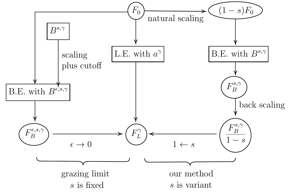
Figure 1. Grazing limit VS our method

In the following, we will explain in more details about the new appraoch. Let $\tilde{F}^{s,\gamma}_{B}=F^{s,\gamma}_{B}/(1-s)$. Then $\tilde{F}^{s,\gamma}_{B}$ is the solution to

$$\partial_{t}F+v\cdot\nabla_{x}F=\tilde{Q}^{s,\gamma}_{B}(F,F),\quad F|_{t=0}=F_{0}.$$ (1.8)

Here $\tilde{Q}^{s,\gamma}_{B}$ is the Boltzmann operator defined with the kernel

$$\tilde{B}^{s,\gamma}(v-v_{*},\sigma)=(1-s)B^{s,\gamma}(v-v_{*},\sigma).$$ (1.9)

In order to prove the limit (1.7), it is equivalent to prove that

$$\tilde{F}^{s,\gamma}_{B}\to F_{L}^{\gamma},\quad s\to 1^{-}.$$ (1.10)

The factor $(1-s)$ that naturally appears in (1.9) corresponds to the grazing limit. This is because only small deviation collisions contribute in the limit $s\to 1^{-}$.

In this paper, we will investigate the above limit in the near-equilibrium framework where the unique global classical solution can be constructed. We first recall some relevant results on the well-posedness theories in this framework. For the non-cutoff kernel (1.6), Gressman-Strain in [15] established global well-posedness of the Boltzmann equation in the following parameter range

$$\gamma>-3,\quad 0<s<1.$$ (1.11)

Independently, Alexandre-Morimoto-Ukai-Xu-Yang [2] proved the same result in the range (1.11) with a constraint $\gamma+2s>-\frac{3}{2}$ to obtain a better estimate on the nonlinear operators. In order to consider the grazing limit for Coulomb potential $\gamma=-3$, we need to obtain some uniform estimates for $\gamma<-3$. There are some discussions about this in the previous works. For instance, the weak solutions were constructed for $\gamma\geq-3$ for the two types of equation in the classical work [32] by Villani in which a remark on page 284 says that ’one could take $\gamma>-4$’. As for Landau equation, Guo [16] firstly proved global well-posedness of for $\gamma\geq-3$ and he pointed out on page 394 in [16] that ’Although our theorem is still valid for certain $\gamma$ even below $-3$’.

Motivated by the above works, we will consider the range $\gamma\leq-3$ in this paper. The new contribution of this paper to the Boltzmann equation is to contain the parameters range for $\gamma$ and $s$ in the triangle $0<s<1,-3-2s<\gamma\leq-3$, see the region formed by the three red dash lines in Figure 2. On one hand, we justisfy the well-posedness of the Boltzmann equation in a region below $\gamma=-3$. On the other hand, more importantly, the uniform estimates are obtained to the left of the vertical line $s=1$ so that the limit $s\to 1^{-}$ can be considered for any $\gamma>-5$. This then obvious includes the Coulomb potential $\gamma=-3$ and the cases mentioned in the previous literatures. Hence, as a byproduct, our new contribution for the Landau equation is the well-posedness for $-5<\gamma<-3$.

Figure 2. The parameters domain

Now let us explain why $\gamma=-2s-3$ is a valid threshold in three dimensional space. It is now well known that the Boltzmann operator $Q^{s,\gamma}_{B}(g,\cdot)$ in (1.5) behaves like a fractional Laplace operator $-C_{g}(-\Delta)^{s}$. Recall that $-(-\Delta)^{s}$ in three dimensions can be defined by a singular integral

$$-(-\Delta)^{s}f(v):=C_{s}\lim_{r\to 0^{+}}\int_{\mathbb{R}^{3}\setminus B(v,r)}\frac{f(v)-f(v_{*})}{|v-v_{*}|^{3+2s}}\mathrm{d}v_{*}.$$ (1.12)

This implies that $\gamma>-2s-3$ for suitably general function spaces. Moreover, there exists a universal constant $c>0$ such that

$$\lim_{s\to 1^{-}}\frac{C_{s}}{1-s}=c.$$

This implies the scaling factor $1-s$ naturally appears in (1.7). Then as $s\to 1^{-}$, $-(-\Delta)^{s}\to\Delta$ which is the main part of the Landau operator (1.2).

1.2. Main results

We will state the main results in this subsection. Consider the following Cauchy problem of the Boltzmann equation

$$\left\{\begin{aligned} &\partial_{t}F+v\cdot\nabla_{x}F=Q^{s,\gamma}_{B}(F,F),~{}~{}t>0,x\in\mathbb{T}^{3},v\in\mathop{\mathbb{R}\kern 0.0pt}\nolimits^{3},\\ &F|_{t=0}=F_{0}.\end{aligned}\right.$$ (1.13)

Here $F(t,x,v)\geq 0$ is the density function of particles with velocity $v\in\mathop{\mathbb{R}\kern 0.0pt}\nolimits^{3}$ at time $t\geq 0$, position $x\in\mathbb{T}^{3}:=[-\pi,\pi]^{3}$. The Boltzmann operator is defined as

$$Q^{s,\gamma}_{B}(g,h)(v):=\int_{\mathop{\mathbb{R}\kern 0.0pt}\nolimits^{3}}\int_{\mathbb{S}^{2}}B^{s,\gamma}(v-v_{*},\sigma)\left(g^{\prime}_{*}h^{\prime}-g_{*}h\right)\mathrm{d}\sigma\mathrm{d}v_{*}.$$ (1.14)

Here, $h=h(v)$, $g_{*}=g(v_{*})$, $h^{\prime}=h(v^{\prime})$, $g^{\prime}_{*}=g(v^{\prime}_{*})$ where $v^{\prime}$, $v_{*}^{\prime}$ are given by

$$v^{\prime}=\frac{v+v_{*}}{2}+\frac{|v-v_{*}|}{2}\sigma,\quad v^{\prime}_{*}=\frac{v+v_{*}}{2}-\frac{|v-v_{*}|}{2}\sigma,\quad\sigma\in\mathbb{S}^{2}.$$ (1.15)

Recalling (1.6) and (1.9), from now on we take

$$B^{s,\gamma}(v-v_{*},\sigma)=(1-s)(\sin\frac{\theta}{2})^{-2-2s}\mathrm{1}_{0\leq\theta\leq\pi/2}|v-v_{*}|^{\gamma},$$ (1.16)

where $\cos\theta=\frac{v-v_{*}}{|v-v_{*}|}\cdot\sigma$. That is, the angular function is

$$b^{s}(\theta)=(1-s)(\sin\frac{\theta}{2})^{-2-2s}\mathrm{1}_{0\leq\theta\leq\pi/2}.$$

Note that the angle variable is restricted to $0\leq\theta\leq\pi/2$ by symmetry as other papers. Thanks to the factor $1-s$, the mean moment transfer is finite by computing

$$\int_{\mathbb{S}^{2}}b^{s}(\theta)\sin^{2}\frac{\theta}{2}\mathrm{d}\sigma=4\pi\times 2^{s-1}.$$ (1.17)

In accordance with (1.17), we take $\Lambda=\pi$ in (1.3). In fact, we will show that

$$Q^{s,\gamma}_{B}=2^{s-1}Q^{\gamma}_{L}+O(1-s),$$

and so $Q^{s,\gamma}_{B}\to Q^{\gamma}_{L}$ as $s\to 1^{-}$. See (7) for details.

To construct the global-in-time classical solution in the spatially inhomogeneous case, one usually consider the near equilibrium framework. Recall that the solution of (1.1) and (1.13) conserves mass, momentum and energy. We assume $F_{0}$ is a small perturbation of the equilibrium $\mu$ where $\mu(v):=(2\pi)^{-3/2}e^{-|v|^{2}/2}$. Let us recall the linearized versions of (1.13) and (1.1). Set $F=\mu+\mu^{1/2}f$, then (1.13) is reduced to

$$\left\{\begin{aligned} &\partial_{t}f+v\cdot\nabla_{x}f+\mathcal{L}^{s,\gamma}_{B}f=\Gamma^{s,\gamma}_{B}(f,f),~{}~{}t>0,x\in\mathbb{T}^{3},v\in\mathop{\mathbb{R}\kern 0.0pt}\nolimits^{3},\\ &f|_{t=0}=f_{0}.\end{aligned}\right.$$ (1.18)

Here the linearized Boltzmann operator $\mathcal{L}^{s,\gamma}_{B}$ and the nonlinear term $\Gamma^{s,\gamma}_{B}$ are defined by

$$\Gamma^{s,\gamma}_{B}(g,h):=\mu^{-1/2}Q^{s,\gamma}_{B}(\mu^{1/2}g,\mu^{1/2}h),\quad\mathcal{L}^{s,\gamma}_{B}g:=-\Gamma^{s,\gamma}_{B}(\mu^{1/2},g)-\Gamma^{s,\gamma}_{B}(g,\mu^{1/2}).$$ (1.19)

With the same decomposition, set $F=\mu+\mu^{1/2}f$. Then (1.1) becomes

$$\left\{\begin{aligned} &\partial_{t}f+v\cdot\nabla_{x}f+\mathcal{L}_{L}^{\gamma}f=\Gamma_{L}^{\gamma}(f,f),t>0,x\in\mathbb{T}^{3},v\in\mathop{\mathbb{R}\kern 0.0pt}\nolimits^{3},\\ &f|_{t=0}=f_{0}.\end{aligned}\right.$$ (1.20)

The linearized Landau operator $\mathcal{L}_{L}^{\gamma}$ and the nonlinear term $\Gamma_{L}^{\gamma}$ are defined by

$$\Gamma_{L}^{\gamma}(g,h):=\mu^{-1/2}Q_{L}^{\gamma}(\mu^{1/2}g,\mu^{1/2}h),\quad\mathcal{L}_{L}^{\gamma}g:=-\Gamma_{L}^{\gamma}(\mu^{1/2},g)-\Gamma_{L}^{\gamma}(g,\mu^{1/2}).$$ (1.21)

Note that the conservation laws imply that for all $t\geq 0$,

$$\int_{\mathbb{T}^{3}\times\mathop{\mathbb{R}\kern 0.0pt}\nolimits^{3}}F(t,x,v)\phi(v)\mathrm{d}x\mathrm{d}v=\int_{\mathbb{T}^{3}\times\mathop{\mathbb{R}\kern 0.0pt}\nolimits^{3}}F(0,x,v)\phi(v)\mathrm{d}x\mathrm{d}v,\quad\phi(v)=1,v_{j},|v|^{2},\quad j=1,2,3.$$ (1.22)

Up to suitable choice of the physical parameters in the equilibrium state, without loss of generality, we assume the initial data satisfy

$$\int_{\mathbb{T}^{3}\times\mathop{\mathbb{R}\kern 0.0pt}\nolimits^{3}}\sqrt{\mu}f_{0}\phi\mathrm{d}x\mathrm{d}v=0,\quad\phi(v)=1,v_{j},|v|^{2},\quad j=1,2,3,\quad F_{0}=\mu+\mu^{\frac{1}{2}}f_{0}\geq 0.$$ (1.23)

Then

$$\int_{\mathbb{T}^{3}\times\mathop{\mathbb{R}\kern 0.0pt}\nolimits^{3}}\sqrt{\mu}f(t)\phi\mathrm{d}x\mathrm{d}v=0,\quad\phi(v)=1,v_{j},|v|^{2},\quad j=1,2,3.$$ (1.24)

The case for hard potential with $\gamma+2s\geq 0$ is relatively easy because the linearized Boltzmann operator has a spectrum gap. This corresponds to the region above the blue line in Figure 2. Therefore, we only consider the soft potentials in this paper when

$$0<s<1,\quad-3<\gamma+2s\leq 0.$$ (1.25)

Note that this corresponds to the region inside the parallelogram in Figure 2. To overcome the lack of spectrum gap, the following weighted energy space is introduced by Guo for the global well-posedness

$$\mathcal{E}_{N,l}^{s,\gamma}(f):=\sum_{j=0}^{N}\|f\|^{2}_{H^{N-j}_{x}\dot{H}^{j}_{l+j(\gamma+2s)}}.$$ (1.26)

If $s=1$, we sometimes write $\mathcal{E}_{N,l}^{\gamma}(f)=\mathcal{E}_{N,l}^{1,\gamma}(f)$ which is the functional space for the Landau equation, cf. Subsection 1.3.

There are three main results given in the following theorem. The first one is the global well-posedness of the Boltzmann equation (1.18) in the parameter range (1.25). The second one is the global well-posedness of the Landau equation (1.20) for $\gamma>-5$. The last one is about the grazing limit of the Boltzmann equation (1.18) to the Landau equation (1.20) by proving a global-in-time asymptotic formula for the limit $s\to 1^{-}$.

Theorem 1.1.

[Well-posedness of the Boltzmann equation] Let $0<s<1,-3<\gamma+2s\leq 0$. Let $N\geq 4,l\geq-N(\gamma+2s)$. There is a constant $\delta_{s,\gamma,N,l}>0$ such that, if

$$\mathcal{E}^{s,\gamma}_{N,l}(f_{0})\leq\delta_{s,\gamma,N,l},$$ (1.27)

then (1.18) admits a unique global solution $f^{s,\gamma}$ satisfying $\mu+\mu^{\frac{1}{2}}f^{s,\gamma}\geq 0$ and

$$\sup_{t\geq 0}\mathcal{E}^{s,\gamma}_{N,l}(f^{s,\gamma}({t}))\leq Z_{s,\gamma,N,l}\mathcal{E}^{s,\gamma}_{N,l}(f_{0}),$$ (1.28)

for some constant $Z_{s,\gamma,N,l}$. Here $\delta_{s,\gamma,N,l}=\frac{1}{2}\eta_{s,\gamma,N,l}^{2}$ where $\eta_{s,\gamma,N,l}$ is given in Theorem 6.1. See (6.9) for the definition of $Z_{s,\gamma,N,l}$. For any fixed $N,l$, there are two functions $\delta_{N,l},Z_{N,l}:(0,1]\times(0,3]\to(0,\infty)$ satisfying

$$\delta_{s,\gamma,N,l}=\delta_{N,l}(s,\gamma+2s+3),\quad Z_{s,\gamma,N,l}=Z_{N,l}(s,\gamma+2s+3),$$ (1.29)

and

$$\delta_{N,l}(x_{1},x_{2})\text{ is non-decreasing w.r.t. each argument, and vanishes as }x_{1}\to 0^{+}\text{ or }x_{2}\to 0^{+},$$ (1.30)

$$Z_{N,l}(x_{1},x_{2})\text{ is non-increasing w.r.t. each argument and tends to infinity as }x_{1}\to 0^{+}\text{ or }x_{2}\to 0^{+}.$$ (1.31)

[Well-posedness of the Landau equation] Taking $s=1$ in the above, the global well-posedness of (1.20) holds true. We state this result in details for later discussion. Let $-3<\gamma+2<0$. Let $N\geq 4,l\geq-N(\gamma+2)$. Suppose $f_{0}$ verify (1.23). Let $\delta_{\gamma,N,l}=\delta_{1,\gamma,N,l},Z_{\gamma,N,l}=Z_{1,\gamma,N,l}$. If

$$\mathcal{E}^{\gamma}_{N,l}(f_{0})\leq\delta_{\gamma,N,l},$$ (1.32)

then (1.20) admits a unique global solution $f^{\gamma}$ satisfying $\mu+\mu^{\frac{1}{2}}f^{\gamma}\geq 0$ and

$$\sup_{t\geq 0}\mathcal{E}^{\gamma}_{N,l}(f^{\gamma}({t}))\leq Z_{\gamma,N,l}\mathcal{E}^{\gamma}_{N,l}(f_{0}).$$ (1.33)

[Asymptotic formula of the grazing limit] Fix $-5<\gamma<-2$. Let $N\geq 4,l\geq-N(\gamma+2)$. Let $s_{*}:=\frac{1}{2}(1-\frac{\gamma+3}{2})$. Assume

$$\mathcal{E}^{\gamma}_{N+3,l+2N-3\gamma+5}(f_{0})\leq\delta_{s_{*},\gamma,N+3,l+2N-3\gamma+5}.$$ (1.34)

Since for any $s_{*}\leq s\leq 1$,

$$\mathcal{E}^{s,\gamma}_{N+3,l+2N-3\gamma+5}(f_{0})\leq\mathcal{E}^{\gamma}_{N+3,l+2N-3\gamma+5}(f_{0})\leq\delta_{s_{*},\gamma,N+3,l+2N-3\gamma+5}\leq\delta_{s,\gamma,N+3,l+2N-3\gamma+5},$$

then by the above well-posedness result, (1.18) has a unique solution $f^{s,\gamma}$ for $s_{*}\leq s<1$, and (1.20) has a unique solution $f^{\gamma}$. Moreover, the family of solutions $\{f^{s,\gamma}\}_{s_{*}\leq s<1}$ satisfy

$$\sup_{t\geq 0}\mathcal{E}^{\gamma}_{N,l}(f^{s,\gamma}(t)-f^{\gamma}(t))\leq(1-s)^{2}Z_{s_{*},\gamma,N,l}\exp\left(C_{N,l}Z_{s_{*},\gamma,N,l}^{3}C_{\gamma}^{2}\mathcal{E}_{N+3,l+2N-3\gamma+5}^{1,\gamma}(f_{0})\right).$$ (1.35)

In the following we will give some remarks on the above result. First of all, we will keep track of the dependence on the parameters $s,\gamma$. This kind of dependence gives the precise condition on the parameters for the global well-posedness theory of the Boltzmann and Landau equation. In particular, we have the explicit relation between $\delta,Z$ and $s,\gamma$ in (1.29). On one hand, the region of parameters for the well-posedness is non-empty as long as $0<s<1,\gamma>-2s-3$. On the other hand, according to (1.30), the region indicated by the ”radius” $\delta_{s,\gamma,N,l}>0$ may shrink as $s\to 0^{+}$ or $\gamma\to(-2s-3)^{+}$.

The estimate (1.35) implies that

$$F^{s,\gamma}_{B}=F^{\gamma}_{L}+(1-s)F_{R}^{s,\gamma},$$ (1.36)

where $F^{s,\gamma}_{B}$ and $F^{\gamma}_{L}$ are solutions to (1.13) and (1.1) respectively. Here the error term $F_{R}^{s,\gamma}$ is uniformly bounded in some function space. The formula validates our approach shown in Figure 1.

A few more remarks are given as follows.

Remark 1.1.

If $s$ and $\gamma$ are regarded as two independent parameters, the well-posedness of the Boltzmann equation holds when $\gamma>-3-2s$ and $0<s<1$. In fact, the angular singularity $s\to 1^{-}$ is the essential reason for being possible ill-posedness.

Remark 1.2.

The global well-posedness in the lower regularity function spaces, such as the one introduced in [13] and time decay rates as in [27, 28, 13] for different non-optimal ranges of the parameters $\gamma$ and $s$ can be obtained for the parameters in the optimal range as in Theorem 1.1. For brevity and to focus on the key points in this paper, we will not pursue these analysis here.

Remark 1.3.

In the previous studies, the reason that the condition $\gamma>-3$ is needed is because the following estimate is used,

$$\int_{\mathbb{R}^{3}}\mu(v_{*})|v-v_{*}|^{\gamma}\mathrm{d}v_{*}\leq C_{\gamma}\langle v\rangle^{\gamma},$$ (1.37)

where $C_{\gamma}$ is a constant for any $v\in\mathbb{R}^{3}$. To understand why $\gamma>-3-2s$ is sufficient for well-posedness, intuitively, one can note the angular singularity in the cross-section leads to a fractional derivative of order $2s$. Thus, we can expect to recover of an extra $2s$ in the range for $\gamma$ below $\gamma=-3$ by sacrificing some regularity of the solution under consideration.

1.3. Notations

We list some notations that are used in the paper.

Common notations. We denote the multi-index $\beta=(\beta_{1},\beta_{2},\beta_{3})$ with $|\beta|=\beta_{1}+\beta_{2}+\beta_{3}$. $a\lesssim b$ means that there is a uniform constant $C,$ which may be different on different lines, such that $a\leq Cb$. We use the notation $a\sim b$ when $a\lesssim b$ and $b\lesssim a$. The bracket $\langle\cdot\rangle$ is defined by $\langle\cdot\rangle:=(1+|\cdot|^{2})^{1/2}$. The weight function $W_{l}$ is defined by $W_{l}(v):=\langle v\rangle^{l}$. We denote $C(\lambda_{1},\lambda_{2},\cdots,\lambda_{n})$ or $C_{\lambda_{1},\lambda_{2},\cdots,\lambda_{n}}$ by a constant depending on parameters $\lambda_{1},\lambda_{2},\cdots,\lambda_{n}$. The notations $\langle f,g\rangle:=\int_{\mathop{\mathbb{R}\kern 0.0pt}\nolimits^{3}}f(v)g(v)\mathrm{d}v$ and $(f,g):=\int_{\mathop{\mathbb{R}\kern 0.0pt}\nolimits^{3}\times\mathop{\mathbb{T}\kern 0.0pt}\nolimits^{3}}fg\mathrm{d}x\mathrm{d}v$ are used to denote the inner products for the $v$ variable and for the $x,v$ variables respectively. As usual, $\mathrm{1}_{A}$ is the characteristic function of the set $A$. If $A,B$ are two operators, then $[A,B]:=AB-BA$.

Function spaces. For simplicity, set $\partial^{\alpha}:=\partial^{\alpha}_{x},\partial_{\beta}:=\partial^{\beta}_{v},\partial^{\alpha}_{\beta}:=\partial^{\alpha}_{x}\partial^{\beta}_{v}$. We will use the following function spaces.

• For real number $n,l$,

  $$H^{n}_{l}:=\bigg{\{}f(v)\big{|}|f|^{2}_{H^{n}_{l}}:=|\langle D\rangle^{n}W_{l}f|^{2}_{L^{2}}=\int_{\mathop{\mathbb{R}\kern 0.0pt}\nolimits^{3}}|(\langle D\rangle^{n}W_{l}f)(v)|^{2}\mathrm{d}v<+\infty\bigg{\}}.$$

  Here $a(D)$ is a differential operator with the symbol $a(\xi)$ defined by

  $$\big{(}a(D)f\big{)}(v):=\frac{1}{(2\pi)^{3}}\int_{\mathop{\mathbb{R}\kern 0.0pt}\nolimits^{3}}\int_{\mathop{\mathbb{R}\kern 0.0pt}\nolimits^{3}}e^{i(v-y)\xi}a(\xi)f(y)\mathrm{d}y\mathrm{d}\xi.$$

• For $n\in\mathop{\mathbb{N}\kern 0.0pt}\nolimits,l\in\mathop{\mathbb{R}\kern 0.0pt}\nolimits$,

  $$H^{n}_{l}:=\bigg{\{}f(v)\big{|}|f|^{2}_{H^{n}_{l}}:=\sum_{|\beta|\leq n}|\partial_{\beta}f|^{2}_{L^{2}_{l}}<\infty\bigg{\}},$$

  where $|f|_{L^{2}_{l}}:=|W_{l}f|_{L^{2}}$ is the usual $L^{2}$ norm with weight $W_{l}$.

• For $n\in\mathop{\mathbb{N}\kern 0.0pt}\nolimits,l\in\mathop{\mathbb{R}\kern 0.0pt}\nolimits$,

  $$\dot{H}^{n}_{l}:=\bigg{\{}f(v)\big{|}|f|^{2}_{\dot{H}^{n}_{l}}:=\sum_{|\beta|=n}|\partial_{\beta}f|^{2}_{L^{2}_{l}}<\infty\bigg{\}}.$$ (1.38)

• For $m\in\mathop{\mathbb{N}\kern 0.0pt}\nolimits$,

  $$H^{m}_{x}:=\bigg{\{}f(x)\big{|}|f|^{2}_{H^{m}_{x}}:=\sum_{|\alpha|\leq m}|\partial^{\alpha}f|^{2}_{L^{2}_{x}}<\infty\bigg{\}}.$$

• For $m,n\in\mathop{\mathbb{N}\kern 0.0pt}\nolimits,l\in\mathop{\mathbb{R}\kern 0.0pt}\nolimits$,

  $$H^{m}_{x}H^{n}_{l}:=\bigg{\{}f(x,v)\big{|}\|f\|^{2}_{H^{m}_{x}H^{n}_{l}}:=\sum_{|\alpha|\leq m,|\beta|\leq n}||\partial^{\alpha}_{\beta}f|_{L^{2}_{l}}|^{2}_{L^{2}_{x}}<\infty\bigg{\}}.$$

  We write $\|f\|_{H^{m}_{x}L^{2}_{l}}:=\|f\|_{H^{m}_{x}L^{2}_{l}}$ if $n=0$ and $\|f\|_{L^{2}_{x}L^{2}_{l}}:=\|f\|_{H^{0}_{x}H^{0}_{l}}$ if $m=n=0$. The space $H^{m}_{x}\dot{H}^{n}_{l}$ can be defined similarly.

Finally in the introduction, let us recall the dissipation norm of the linearized operators $\mathcal{L}^{s,\gamma}_{B}$ and $\mathcal{L}^{\gamma}_{L}$. More precisely, for $l\in\mathbb{R}$, set

$$|f|^{2}_{s,l}:=|W_{s}((-\Delta_{\mathbb{S}^{2}})^{1/2})W_{l}f|^{2}_{L^{2}}+|W_{s}(D)W_{l}f|^{2}_{L^{2}}+|W_{s}W_{l}f|^{2}_{L^{2}}.$$ (1.39)

Here $W_{s}(D)$ is the pseudo-differential operator with symbol $W_{s}$. The operator $W_{s}((-\Delta_{\mathbb{S}^{2}})^{1/2})$ is defined as follows. If $v=r\sigma,r\geq 0,\sigma\in\mathbb{S}^{2}$, then

$$(W_{s}((-\Delta_{\mathbb{S}^{2}})^{1/2})f)(v):=\sum_{l=0}^{\infty}\sum_{m=-l}^{l}(1+l(l+1))^{\frac{s}{2}}Y^{m}_{l}(\sigma)f^{m}_{l}(r),$$ (1.40)

where $f^{m}_{l}(r)=\int_{\mathbb{S}^{2}}Y^{m}_{l}(\sigma)f(r\sigma)\mathrm{d}\sigma$, and $Y_{l}^{m},-l\leq m\leq l$ are the real spherical harmonics satisfying $(-\Delta_{\mathbb{S}^{2}})Y_{l}^{m}=l(l+1)Y_{l}^{m}.$ Note that the function $W_{s}$ is the common weight gain in the three individual norms. The dissipation norm $|\cdot|_{s,\gamma/2}$ characterizes $\mathcal{L}^{s,\gamma}_{B}$, see Proposition 3.8 and Theorem 4.2 for details. Similarly, the dissipation norm $|\cdot|_{1,\gamma/2}$ characterizes the $\mathcal{L}^{\gamma}_{L}$.

From time to time, we also write $|f|_{L^{2}_{s,l}}=|f|_{s,l}$. For functions defined on $\mathbb{T}^{3}\times\mathop{\mathbb{R}\kern 0.0pt}\nolimits^{3}$, the space $H^{m}_{x}H^{n}_{s,l}$ with $m,n\in\mathop{\mathbb{N}\kern 0.0pt}\nolimits$ is defined by

$$H^{m}_{x}H^{n}_{s,l}:=\bigg{\{}f(x,v)\big{|}\|f\|^{2}_{H^{m}_{x}H^{n}_{s,l}}:=\sum_{|\alpha|\leq m,|\beta|\leq n}||\partial^{\alpha}_{\beta}f|_{L^{2}_{s,l}}|^{2}_{L^{2}_{x}}<\infty\bigg{\}}.$$

Set $\|f\|_{H_{x}^{m}L^{2}_{s,l}}:=\|f\|_{H^{m}_{x}H^{0}_{s,l}}$ if $n=0$ and $\|f\|_{L^{2}_{x}L^{2}_{s,l}}:=\|f\|_{H^{0}_{x}H^{0}_{s,l}}$ if $m=n=0$. Again, the space $H^{m}_{x}\dot{H}^{n}_{s,l}$ can be defined accordingly.

We sometimes omit the range of some frequently used variables in the integrals. Usually, $\sigma\in\mathbb{S}^{2},v,v_{*},u,\xi\in\mathbb{R}^{3}$. For example, $\int(\cdots)\mathrm{d}\sigma:=\int_{\mathbb{S}^{2}}(\cdots)\mathrm{d}\sigma,\int(\cdots)\mathrm{d}\sigma\mathrm{d}v\mathrm{d}v_{*}:=\int_{\mathbb{S}^{2}\times\mathbb{R}^{3}\times\mathbb{R}^{3}}(\cdots)\mathrm{d}\sigma\mathrm{d}v\mathrm{d}v_{*}$. Integration w.r.t. other variables is understood in a similar way. Whenever a new variable appears, we will specify its range.

When there is no confusion, we drop the subscripts $B$ and $L$ in the Boltzmann and Landau operators for brevity.

1.4. Organization of the paper

In Section 2, we derive the upper bound estimates of operators in the singular region. Section 3 contains the upper bound estimates in the regular region. We will show the coercivity estimate in Section 4. The commutator estimates and weighted upper bound estimates are given in Section 5. The proof Theorem 1.1 is given in Section 6. In the Appendix 7, for completeness, we prove the operator convergence stated in Proposition 6.2.

2. Upper bound estimate in the singular region

In this section, we will derive the upper bound estimates on the collision operators in the singular region $|v-v_{*}|\lesssim\eta$. For this, we first recall the dyadic decomposition.

2.1. Dyadic decomposition

Let $\varphi$ be a smooth function on $\mathbb{R}_{+}$ satisfying

$$\varphi=0\text{ on }[0,3/4],\quad\varphi\text{ is strictly increasing on }[3/4,4/3],\quad\varphi=1\text{ on }[4/3,3/2],$$

$$\varphi\text{ is strictly decreasing on }[3/2,8/3],\quad\varphi=0\text{ on }[8/3,\infty),\quad|\varphi^{\prime}|\leq 4.$$

Moreover, $\varphi$ is chosen such that the functions $\{\varphi_{k}(\cdot)\colonequals\varphi(\cdot/2^{k})\}_{k\in\mathbb{Z}}$ is a partition of unit on $(0,\infty)$. That is,

$$\sum_{k=-\infty}^{\infty}\varphi_{k}=1\text{ on }(0,\infty).$$ (2.1)

Set $\psi(r)=\sum_{k=-\infty}^{-1}\varphi_{k}(r)$ for $r>0$ and $\psi(0)=1$. Then $\psi$ is a non-increasing smooth function on $\mathbb{R}_{+}$ and satisfies

$$\psi=1\text{ on }[0,3/4],\quad\psi\text{ is strictly decreasing on }[3/4,4/3],\quad\psi=0\text{ on }[4/3,\infty),\quad|\psi^{\prime}|\leq 4.$$ (2.2)

Then we have the identity

$$\psi+\sum_{k=0}^{\infty}\varphi_{k}\equiv 1\text{ on }[0,\infty).$$ (2.3)

With a little abuse of notation, we define radial functions $\varphi(v)\colonequals\varphi(|v|),\psi(v)\colonequals\psi(|v|),\varphi_{k}(v)\colonequals\varphi_{k}(|v|)$ for $v\in\mathop{\mathbb{R}\kern 0.0pt}\nolimits^{3}$.

Given a general Boltzmann kernel $B=B(v-v_{*},\sigma)=B(|v-v_{*}|,\cos\theta)$ where $\cos\theta=\frac{v-v_{*}}{|v-v_{*}|}\cdot\sigma$, let $Q$ be the Boltzmann operator with kernel $B$. That is,

$$Q(g,h)\colonequals\int_{\mathbb{S}^{2}}\int_{\mathbb{R}^{3}}B(|v-v_{*}|,\frac{v-v_{*}}{|v-v_{*}|}\cdot\sigma)(g^{\prime}_{*}h^{\prime}-g_{*}h)\mathrm{d}\sigma\mathrm{d}v_{*}.$$ (2.4)

Let $\mathcal{U}_{k}\colonequals\sum_{j\leq k}\varphi_{j},\tilde{\varphi}_{k}\colonequals\sum_{|j-k|\leq N_{0}-1}\varphi_{j}$ for $k\in\mathbb{Z}$ for some fixed integer $N_{0}\geq 4$. Suppose the relative velocity satisfies $|v-v_{*}|\leq\frac{4}{3}$. Let $v_{*}\in\{\frac{3}{4}\times 2^{j}\leq|v_{*}|\leq\frac{8}{3}\times 2^{j}\}$. Then the fact that

$$\frac{\sqrt{2}}{2}|v-v_{*}|\leq|v^{\prime}-v_{*}|\leq|v-v_{*}|,$$

yields

• If $j\geq N_{0}-1$, then $|v|,|v^{\prime}|\in[(\frac{3}{4}-\frac{8}{3}\times 2^{-N_{0}})2^{j},\frac{8}{3}(1+2^{-N_{0}})2^{j}]\subset\mathrm{Supp}\tilde{\varphi}_{j}$.

• If $j\leq N_{0}-2$, then $|v|,|v^{\prime}|\leq\frac{3}{2}\times 2^{N_{0}-1}\subset\mathrm{Supp}\mathcal{U}_{N_{0}-1}$.

Hence, if $Q$ is localized in $|v-v_{*}|\leq\frac{4}{3}$, then

$$\langle Q(g,h),f\rangle=\sum_{j\geq N_{0}-1}\langle Q(\varphi_{j}g,\tilde{\varphi}_{j}h),\tilde{\varphi}_{j}f\rangle+\langle Q(\mathcal{U}_{N_{0}-2}g,\mathcal{U}_{N_{0}-1}h),\mathcal{U}_{N_{0}-1}f\rangle.$$ (2.5)

Let us recall the Bobylev formula which is about the Fourier transform of the Boltzmann operator. By (2.4), the Bobylev formula reads

$$\mathcal{F}(Q(g,h))(\xi)=\int_{\mathbb{S}^{2}}\int_{\mathbb{R}^{3}}\big{(}\hat{B}(|\eta_{*}-\xi^{-}|,\frac{\xi}{|\xi|}\cdot\sigma)-\hat{B}(|\eta_{*}|,\frac{\xi}{|\xi|}\cdot\sigma)\big{)}\mathcal{F}g(\eta_{*})\mathcal{F}h(\xi-\eta_{*})\mathrm{d}\sigma\mathrm{d}\eta_{*},$$

where

$$\hat{B}(|\xi|,\cos\theta)\colonequals\int_{\mathbb{R}^{3}}B(|q|,\cos\theta)e^{-iq\cdot\xi}\mathrm{d}q.$$

Here $\mathcal{F}$ is the Fourier transform operator. As usual, denote $\hat{f}=\mathcal{F}f$, then

$$\langle Q(g,h),f\rangle = \langle\widehat{Q(g,h)},\hat{f}\rangle$$ (2.6)

$$= \int_{\mathbb{S}^{2}}\int_{\mathbb{R}^{3}}\int_{\mathbb{R}^{3}}\big{(}\hat{B}(|\eta_{*}-\xi^{-}|,\frac{\xi}{|\xi|}\cdot\sigma)-\hat{B}(|\eta_{*}|,\frac{\xi}{|\xi|}\cdot\sigma)\big{)}\hat{g}(\eta_{*})\hat{h}(\xi-\eta_{*})\bar{\hat{f}}(\xi)\mathrm{d}\sigma\mathrm{d}\eta_{*}\mathrm{d}\xi.$$

Note that

$$||\xi|-|\eta_{*}||\leq|\xi-\eta_{*}|\leq|\xi|+|\eta_{*}|.$$

Fix $j,p\in\mathbb{Z}$, suppose $\frac{3}{4}\times 2^{p}\leq|\eta_{*}|\leq\frac{8}{3}\times 2^{p}$ and $\frac{3}{4}\times 2^{j}\leq|\xi-\eta_{*}|\leq\frac{8}{3}\times 2^{j}$. Since $N_{0}\geq 4$, then

• If $p\leq j-N_{0}$, then $|\xi|\in[(\frac{3}{4}-\frac{8}{3}\times 2^{-N_{0}})2^{j},\frac{8}{3}(1+2^{-N_{0}})2^{j}]\subset\mathrm{Supp}\tilde{\varphi}_{j}$.

• If $p\geq j+N_{0}$, then $|\xi|\in[(\frac{3}{4}-\frac{8}{3}\times 2^{-N_{0}})2^{p},\frac{8}{3}(1+2^{-N_{0}})2^{p}]\subset\mathrm{Supp}\tilde{\varphi}_{p}$.

• If $|p-j|<N_{0}$, then $|\xi|\in[0,\frac{3}{2}\times 2^{p+N_{0}}]\cap[0,\frac{3}{2}\times 2^{j+N_{0}}]\subset\mathrm{Supp}\mathcal{U}_{p+N_{0}}\cap\mathrm{Supp}\mathcal{U}_{j+N_{0}}$.

Define

$$\mathfrak{F}_{-1}f(x)\colonequals\psi(D)f,\quad\mathfrak{F}_{j}f(x)\colonequals\varphi_{j}(D)f,j\geq 0.$$ (2.7)

$\mathfrak{F}_{-1}$ and $\mathfrak{F}_{j}$ localize the frequency of function $f$ in the region $|\xi|\lesssim 1$ and $|\xi|\sim 2^{j}$ respectively. By (2.3), the dyadic decomposition in frequency space reads

$$f=\sum_{j\geq-1}\mathfrak{F}_{j}f.$$

Note that $\mathfrak{F}_{-1}$ has symbol $\psi$ instead of $\varphi_{-1}$. Set $\tilde{\mathfrak{F}}_{k}:=\tilde{\varphi}_{k}(D)$. Then we have

$$\langle Q(g,h),f\rangle = \sum_{j\geq N_{0}-1}\sum_{-1\leq p\leq j-N_{0}}\langle Q(\mathfrak{F}_{p}g,\mathfrak{F}_{j}h),\tilde{\mathfrak{F}}_{j}f\rangle+\sum_{p\geq N_{0}-1}\sum_{-1\leq j\leq p-N_{0}}\langle Q(\mathfrak{F}_{p}g,\mathfrak{F}_{j}h),\tilde{\mathfrak{F}}_{p}f\rangle$$

$$+\sum_{p,j\geq-1,|p-j|<N_{0}}\sum_{q\leq j+N_{0}}\langle Q(\mathfrak{F}_{p}g,\mathfrak{F}_{j}h),\mathfrak{F}_{q}f\rangle.$$

For completeness, we recall the definition of symbol class $S^{m}_{1,0}$ as follows.

Definition 2.1.

A smooth function $W(v,\xi)$ is said to be a symbol of type $S^{m}_{1,0}$ if for any multi-indices $\alpha$ and $\beta$,

$$|(\partial^{\alpha}_{\xi}\partial^{\beta}_{v}W)(v,\xi)|\leq C_{\alpha,\beta}\langle\xi\rangle^{m-|\alpha|},$$

where $C_{\alpha,\beta}$ is a constant depending only on $\alpha$ and $\beta$.

Lemma 2.1.

Let $l,m,r\in\mathop{\mathbb{R}\kern 0.0pt}\nolimits,M(v,\xi)=M(\xi)\in S^{r}_{1,0}$ and $\Phi(v,\xi)=\Phi(\xi)\in S^{l}_{1,0}$. Then there exists a constant $C$ such that

$$|[M(D),\Phi]f|_{H^{m}}\leq C|f|_{H^{r+s-1}_{l-1}}.$$

See Lemma 5.3 in [22] for the proof of Lemma 2.1. Based on Lemma 2.1, one directly has

$$|f|_{H^{m}_{l}}^{2}\sim\sum_{j,k=-1}^{\infty}2^{2mk}2^{2lj}|\varphi_{k}(D)\varphi_{j}f|_{L^{2}}^{2}\sim\sum_{j,k=-1}^{\infty}2^{2mk}2^{2lj}|\varphi_{j}\varphi_{k}(D)f|_{L^{2}}^{2}.$$ (2.9)

Here for simplicity, we take $\varphi_{-1}:=\psi$. By (2.9), we use both $|W_{l}f|_{H^{m+s}}$ and $|W_{l}W_{s}(D)f|_{H^{m}}$ in the rest of the paper.

2.2. Operator splitting

We divide the relative velocity into two parts

$$B(v-v_{*},\sigma)=B_{\eta}^{s,\gamma}(v-v_{*},\sigma)+B^{s,\gamma,\eta}(v-v_{*},\sigma),$$

where

$$B_{\eta}^{s,\gamma}(v-v_{*},\sigma):=\psi_{\eta}(|v-v_{*}|)B(v-v_{*},\sigma),\quad B^{s,\gamma,\eta}(v-v_{*},\sigma):=(1-\psi_{\eta}(|v-v_{*}|))B(v-v_{*},\sigma).$$ (2.10)

Note that $B^{s,\gamma}_{\eta}$ is supported in $|v-v_{*}|\leq 4\eta/3$ so that it is singular when $|v-v_{*}|\to 0$, while $B^{s,\gamma,\eta}$ is supported in $|v-v_{*}|\geq 3\eta/4$ without singularity.

Let $Q^{s,\gamma}_{\eta}$ and $Q^{s,\gamma,\eta}$ be the Boltzmann operators defined with kernel $B^{s,\gamma}_{\eta}$ and $B^{s,\gamma,\eta}$ respectively. And then let $\Gamma^{s,\gamma}_{\eta}$ and $\Gamma^{s,\gamma,\eta}$ be the nonlinear terms defined with kernel $B^{s,\gamma}_{\eta}$ and $B^{s,\gamma,\eta}$ respectively.

Recall that the nonlinear term $\Gamma$ for a general kernel $B$ is defined by

$$\Gamma(g,h) = \mu^{-1/2}Q(\mu^{1/2}g,\mu^{1/2}h)=\int B(v-v_{*},\sigma)\mu^{1/2}_{*}\big{(}g^{\prime}_{*}h^{\prime}-g_{*}h\big{)}\mathrm{d}\sigma\mathrm{d}v_{*}$$

$$= \int B(v-v_{*},\sigma)\big{(}(\mu^{1/2}g)^{\prime}_{*}h^{\prime}-(\mu^{1/2}g)_{*}h\big{)}\mathrm{d}\sigma\mathrm{d}v_{*}$$

$$+\int B(v-v_{*},\sigma)\big{(}\mu^{1/2}_{*}-(\mu^{1/2})^{\prime}_{*}\big{)}g^{\prime}_{*}h^{\prime}\mathrm{d}\sigma\mathrm{d}v_{*}=Q(\mu^{1/2}g,h)+I(g,h),$$

where for brevity, we define

$$I(g,h):=\int B(v-v_{*},\sigma)\big{(}\mu^{1/2}_{*}-(\mu^{1/2})^{\prime}_{*}\big{)}g^{\prime}_{*}h^{\prime}\mathrm{d}\sigma\mathrm{d}v_{*}.$$ (2.11)

Let $I^{s,\gamma},I^{s,\gamma}_{\eta}$ and $I^{s,\gamma,\eta}$ be the bi-linear operators defined according to (2.11) with kernel $B^{s,\gamma},B^{s,\gamma}_{\eta}$ and $B^{s,\gamma,\eta}$ respectively. Other operators with such subscripts and superscripts are understood in the same way. With these notations, we have

$$\Gamma^{s,\gamma}(g,h) = Q^{s,\gamma}(\mu^{1/2}g,h)+I^{s,\gamma}(g,h),$$ (2.12)

$$\Gamma^{s,\gamma,\eta}(g,h) = Q^{s,\gamma,\eta}(\mu^{1/2}g,h)+I^{s,\gamma,\eta}(g,h),$$ (2.13)

$$\Gamma^{s,\gamma}_{\eta}(g,h) = Q^{s,\gamma}_{\eta}(\mu^{1/2}g,h)+I^{s,\gamma}_{\eta}(g,h),$$ (2.14)

$$Q^{s,\gamma}(g,h) = Q^{s,\gamma,\eta}(g,h)+Q^{s,\gamma}_{\eta}(g,h),$$ (2.15)

$$\Gamma^{s,\gamma}(g,h) = \Gamma^{s,\gamma,\eta}(g,h)+\Gamma^{s,\gamma}_{\eta}(g,h),$$ (2.16)

$$I^{s,\gamma}(g,h) = I^{s,\gamma,\eta}(g,h)+I^{s,\gamma}_{\eta}(g,h).$$ (2.17)

To implement the energy estimates for the nonlinear equations, we need to take derivatives. By binomial expansion, we have

$$\partial^{\alpha}_{\beta}\Gamma^{s,\gamma}(g,h)=\sum_{\beta_{0}+\beta_{1}+\beta_{2}=\beta,\alpha_{1}+\alpha_{2}=\alpha}C^{\beta_{0},\beta_{1},\beta_{2}}_{\beta}C^{\alpha_{1},\alpha_{2}}_{\alpha}\Gamma^{s,\gamma}(\partial^{\alpha_{1}}_{\beta_{1}}g,\partial^{\alpha_{2}}_{\beta_{2}}h;\beta_{0}),$$ (2.18)

where

$$\Gamma^{s,\gamma}(g,h;\beta)(v):=\int_{\SS^{2}\times\mathop{\mathbb{R}\kern 0.0pt}\nolimits^{3}}B^{s,\gamma}(v-v_{*},\sigma)(\partial_{\beta}\mu^{1/2})_{*}(g^{\prime}_{*}h^{\prime}-g_{*}h)\mathrm{d}\sigma\mathrm{d}v_{*}.$$ (2.19)

Note that

$$\Gamma^{s,\gamma}(g,h;\beta)=Q^{s,\gamma}(g\partial_{\beta}\mu^{1/2},h)+I^{s,\gamma}(g,h;\beta),$$ (2.20)

where

$$I^{s,\gamma}(g,h;\beta):=\int B^{s,\gamma}(v-v_{*},\sigma)\big{(}(\partial_{\beta}\mu^{1/2})_{*}-(\partial_{\beta}\mu^{1/2})^{\prime}_{*}\big{)}g^{\prime}_{*}h^{\prime}\mathrm{d}\sigma\mathrm{d}v_{*}.$$ (2.21)

Thus, in general we need to consider $I^{s,\gamma}(g,h;\beta)$. This is again divided into two parts: $I^{s,\gamma,\eta}(g,h;\beta)$ and $I^{s,\gamma}_{\eta}(g,h;\beta)$.

Recall

$$\mathcal{L}^{s,\gamma}f=-\Gamma^{s,\gamma}(\mu^{\frac{1}{2}},f)-\Gamma^{s,\gamma}(f,\mu^{\frac{1}{2}}).$$

By binomial expansion, we have

$$\partial^{\alpha}_{\beta}\mathcal{L}^{s,\gamma}f=\sum_{\beta_{0}+\beta_{1}+\beta_{2}=\beta}C^{\beta_{0},\beta_{1},\beta_{2}}_{\beta}\mathcal{L}^{s,\gamma}(\partial^{\alpha}_{\beta_{2}}f;\beta_{0},\beta_{1}),$$ (2.22)

where

$$\mathcal{L}^{s,\gamma}(f;\beta_{0},\beta_{1}):=-\Gamma^{s,\gamma}(\partial_{\beta_{1}}\mu^{1/2},f;\beta_{0})-\Gamma^{s,\gamma}(f,\partial_{\beta_{1}}\mu^{1/2};\beta_{0}).$$ (2.23)

We also define

$$\mathcal{L}^{s,\gamma}_{1}(f;\beta_{0},\beta_{1}):=-\Gamma^{s,\gamma}(\partial_{\beta_{1}}\mu^{1/2},f;\beta_{0}),\quad\mathcal{L}^{s,\gamma}_{2}(f;\beta_{0},\beta_{1}):=-\Gamma^{s,\gamma}(f,\partial_{\beta_{1}}\mu^{1/2};\beta_{0}).$$ (2.24)

In the same way, we can define $\mathcal{L}^{s,\gamma,\eta}(\cdot;\beta_{0},\beta_{1}),\mathcal{L}^{s,\gamma,\eta}_{1}(\cdot;\beta_{0},\beta_{1}),\mathcal{L}^{s,\gamma,\eta}_{2}(\cdot;\beta_{0},\beta_{1})$ with kernel $B^{s,\gamma,\eta}$ and $\mathcal{L}^{s,\gamma}_{\eta}(\cdot;\beta_{0},\beta_{1}),\mathcal{L}^{s,\gamma}_{\eta,1}(\cdot;\beta_{0},\beta_{1}),\mathcal{L}^{s,\gamma}_{\eta,2}(\cdot;\beta_{0},\beta_{1})$ with kernel $B^{s,\gamma}_{\eta}$.

2.3. Taylor expansion and symmetry

When evaluating the difference $f^{\prime}-f$ (or $f^{\prime}_{*}-f_{*}$) before and after collision, Taylor expansion is applied. We first denote the 1st-order expansion by

$$f^{\prime}-f=\int_{0}^{1}(\nabla f)(v(\kappa))\cdot(v^{\prime}-v)\mathrm{d}\kappa,\quad f^{\prime}_{*}-f_{*}=\int_{0}^{1}(\nabla f)(v_{*}(\iota))\cdot(v^{\prime}_{*}-v_{*})\mathrm{d}\iota.$$ (2.25)

To cancel the angular singularity, the second order expansion is needed:

$$f^{\prime}-f=(\nabla f)(v)\cdot(v^{\prime}-v)+\int_{0}^{1}(1-\kappa)(\nabla^{2}f)(v(\kappa)):(v^{\prime}-v)\otimes(v^{\prime}-v)\mathrm{d}\kappa,$$ (2.26)

$$f^{\prime}-f=(\nabla f)(v^{\prime})\cdot(v^{\prime}-v)-\int_{0}^{1}\kappa(\nabla^{2}f)(v(\kappa)):(v^{\prime}-v)\otimes(v^{\prime}-v)\mathrm{d}\kappa.$$ (2.27)

Thanks to the symmetry property of $\sigma$-integral, we have

$$\int B(|v-v_{*}|,\frac{v-v_{*}}{|v-v_{*}|}\cdot\sigma)(v^{\prime}-v)\mathrm{d}\sigma=\int B(|v-v_{*}|,\frac{v-v_{*}}{|v-v_{*}|}\cdot\sigma)\sin^{2}\frac{\theta}{2}(v_{*}-v)\mathrm{d}\sigma,$$ (2.28)

$$\int B(|v-v_{*}|,\frac{v-v_{*}}{|v-v_{*}|}\cdot\sigma)(v^{\prime}-v)h(v^{\prime})\mathrm{d}\sigma\mathrm{d}v=0.$$ (2.29)

Here, the formula (2.28) holds for fixed $v,v_{*}$ and (2.29) holds for fixed $v_{*}$.

We now recall a useful formula in the following lemma on the change of variables $v\to v(\kappa)$ and $v_{*}\to v_{*}(\iota)$ where for $\kappa,\iota\in[0,1]$,

$$v(\kappa)=\kappa v^{\prime}+(1-\kappa)v,\quad v_{*}(\iota)=\iota v^{\prime}_{*}+(1-\iota)v_{*}.$$ (2.30)

Lemma 2.2.

For $a\in[0,2]$, let us define

$$\psi_{a}(\theta)\colonequals(\cos^{2}\frac{\theta}{2}+(1-a)^{2}\sin^{2}\frac{\theta}{2})^{-1/2}.$$ (2.31)

For any $0\leq\kappa,\iota\leq 1$, it holds that

$$\int_{\mathop{\mathbb{R}\kern 0.0pt}\nolimits^{3}}\int_{\mathop{\mathbb{R}\kern 0.0pt}\nolimits^{3}}\int_{\SS^{2}_{+}}B(|v-v_{*}|,\cos\theta)g(\iota(v_{*}))f(v(\kappa))\mathrm{d}v\mathrm{d}v_{*}\mathrm{d}\sigma$$

$$= \int_{\mathop{\mathbb{R}\kern 0.0pt}\nolimits^{3}}\int_{\mathop{\mathbb{R}\kern 0.0pt}\nolimits^{3}}\int_{\SS^{2}_{+}}B(|v-v_{*}|\psi_{\kappa+\iota}(\theta),\cos\theta)g(v_{*})f(v)\psi_{\kappa+\iota}^{3}(\theta)\mathrm{d}v\mathrm{d}v_{*}\mathrm{d}\sigma.$$

Here $\SS^{2}_{+}$ stands for $(v-v_{*})\cdot\sigma\geq 0$.

Before giving the proof of this lemma, we firstly note that the above formula is general as it simultaneously deals with the two changes $v\to v(\kappa)$ and $v_{*}\to v_{*}(\iota)$. This will be used in the proof of Proposition 6.2. If $\kappa=\iota=0$, then $\psi_{\kappa+\iota}(\theta)=\psi_{0}(\theta)=1$ and it corresponds to the identity transformation. If $\kappa=\iota=1$, then $\psi_{\kappa+\iota}(\theta)=\psi_{2}(\theta)=1$ and it corresponds to the change of velocities for pre-post collision: $(v,v_{*},\sigma)\rightarrow(v^{\prime},v_{*}^{\prime},\sigma^{\prime}=(v-v_{*})/|v-v_{*}|)$. If $\kappa=1,\iota=0$ or $\kappa=0,\iota=1$, then $\psi_{\kappa+\iota}(\theta)=\psi_{1}(\theta)=\cos^{-1}\frac{\theta}{2}$ and it corresponds to $v\to v^{\prime}$ or $v_{*}\to v^{\prime}_{*}$ respectively. This is consistent with the cancellation lemma given in [1]. If $\iota=0$ or $\kappa=0$, then it corresponds to the individual change $v\to v(\kappa)$ or $v_{*}\to v_{*}(\iota)$ respectively.

Note that $1\leq\psi_{a}(\theta)\leq\sqrt{2}$ for $a\in[0,2],\theta\in[0,\pi/2]$. Thanks to Lemma 2.2 and $1\leq\psi_{a}(\theta)\leq\sqrt{2}$, considering the kernel (1.16), we can skip the details regarding the above mentioned change of variables. As a result, in most part of this paper, $v(\kappa)$ and $v_{*}(\iota)$ will be replaced by $v$ and $v_{*}$ respectively at the cost of a multiplicative constant.

Proof of Lemma 2.2.

The case $\kappa=\iota=1$ is obviously given by the standard change of variable $(v,v_{*},\sigma)\to(v^{\prime},v^{\prime}_{*},\sigma^{\prime})$ where $\sigma^{\prime}=(v-v_{*})/|v-v_{*}|$. This change has unit Jacobian.

Now we deal with the case $\kappa+\iota<2$. Recalling (2.30), it is direct to check

$$|v-v_{*}|=|\kappa(v)-\iota(v_{*})|\psi_{\kappa+\iota}(\theta).$$ (2.33)

Let $\beta$ be the angle between $\kappa(v)-\iota(v_{*})$ and $\sigma$, then $\cos\beta=\varphi_{\kappa+\iota}(\sin\frac{\theta}{2})$ where

$$\varphi_{a}(x):=\frac{1-x^{2}+(a-1)x^{2}}{\left(1-x^{2}+(1-a)^{2}x^{2}\right)^{1/2}}.$$

Let $\delta_{a}\colonequals\arccos(\frac{\sqrt{2}}{2}\frac{a}{\sqrt{1+(1-a)^{2}}})$. If $\kappa+\iota<2$, then $\delta_{\kappa+\iota}>0$ and the function: $\theta\in[0,\frac{\pi}{2}]\to\beta_{\kappa+\iota}\in[0,\delta_{\kappa+\iota}]$ is a bijection. It holds that

$$\det(\frac{\partial(\kappa(v),\iota(v_{*}))}{\partial(v,v_{*})})=\alpha_{\kappa+\iota}(\theta),$$ (2.34)

where for $0\leq a\leq 2$,

$$\alpha_{a}(\theta)\colonequals(1-\frac{a}{2})^{2}\left((1-\frac{a}{2})+\frac{a}{2}\cos\theta\right).$$ (2.35)

By (2.33) and (2.34), with $\mathrm{d}\sigma=\sin\beta\mathrm{d}\beta\mathrm{d}\mathbb{S}$, we have

$$\int_{\mathop{\mathbb{R}\kern 0.0pt}\nolimits^{3}}\int_{\mathop{\mathbb{R}\kern 0.0pt}\nolimits^{3}}\int_{\SS^{2}_{+}}B(|v-v_{*}|,\cos\theta)g(\iota(v_{*}))f(v(\kappa))\mathrm{d}v\mathrm{d}v_{*}\mathrm{d}\sigma$$

$$= 2\pi\int_{\mathop{\mathbb{R}\kern 0.0pt}\nolimits^{3}}\int_{\mathop{\mathbb{R}\kern 0.0pt}\nolimits^{3}}\int_{0}^{\delta_{\kappa+\iota}}B(|v-v_{*}|\psi_{\kappa+\iota}(\theta),\cos\theta)g(v_{*})f(v)\alpha_{\kappa+\iota}^{-1}(\theta)\sin\beta\mathrm{d}v\mathrm{d}v_{*}\mathrm{d}\beta.$$

It is directly to check that

$$\alpha_{\kappa+\iota}^{-1}(\theta)\sin\beta\mathrm{d}\beta=-\alpha_{\kappa+\iota}^{-1}(\theta)\mathrm{d}\cos\beta=-\frac{1}{4}\varphi^{\prime}_{\kappa+\iota}(\sin\frac{\theta}{2})\sin^{-1}\frac{\theta}{2}\alpha_{\kappa+\iota}^{-1}(\theta)\sin\theta\mathrm{d}\theta=\psi_{\kappa+\iota}^{3}(\theta)\sin\theta\mathrm{d}\theta.$$

Then we go back from $\beta$ to $\theta$ and use $\mathrm{d}\sigma=\sin\theta\mathrm{d}\theta\mathrm{d}\mathbb{S}$ to get (2.2). ∎

2.4. Upper bound of $Q^{s,\gamma}_{\eta}$

We give the upper bound of $Q^{s,\gamma}_{\eta}$ in the following proposition.

Proposition 2.1.

Let $0<s<1,-2s-3<\gamma\leq 0,0<\eta\leq 1$. Let $l_{1},l_{2},l_{3}\in\mathop{\mathbb{R}\kern 0.0pt}\nolimits$ satisfying $l_{1}+l_{2}+l_{3}=0$. For any fixed small $1/2\geq\delta>0$, for any combination $a_{1},a_{2},a_{3}\geq 0,a_{1}+a_{2}\geq s,a_{1}+a_{3}\geq 2s,a_{2}+a_{3}\geq 2s$ satisfying the constraint $a_{1}+a_{2}+a_{3}=2s+\frac{3}{2}+\delta$, we have

$$|\langle Q^{s,\gamma}_{\eta}(g,h),f\rangle|\lesssim C_{\delta,s,\gamma,\eta}|g|_{H^{a_{1}}_{l_{1}}}|h|_{H^{a_{2}}_{l_{2}}}|f|_{H^{a_{3}}_{l_{3}}},$$

where

$$C_{\delta,s,\gamma,\eta}:=\delta^{-\frac{1}{2}}C_{s,\gamma,\eta},\quad C_{s,\gamma,\eta}:=\frac{1}{s}\frac{\eta^{\gamma+2s+3}}{\gamma+2s+3}.$$ (2.36)

We point out that the constant associated to $\lesssim$ in the above inequality depends only on the upper bound of $|l_{1}|,|l_{2}|,|l_{3}|$.

Proof.

Recalling the decomposition in frequency space, we have

$$\langle Q^{s,\gamma}_{\eta}(g,h),f\rangle = \sum_{j\leq k-N_{0}}\langle Q^{s,\gamma}_{\eta}(\mathfrak{F}_{j}g,\mathfrak{F}_{k}h),\tilde{\mathfrak{F}}_{k}f\rangle+\sum_{|j-k|<N_{0}}\sum_{l\leq k+N_{0}}\langle Q^{s,\gamma}_{\eta}(\mathfrak{F}_{j}g,\mathfrak{F}_{k}h),\mathfrak{F}_{l}f\rangle$$

$$+\sum_{j\geq k+N_{0}}\langle Q^{s,\gamma}_{\eta}(\mathfrak{F}_{j}g,\mathfrak{F}_{k}h),\tilde{\mathfrak{F}}_{j}f\rangle.$$

We estimate the second quantity in details for illustration. That is, when $|j-k|<N_{0},l\leq k+N_{0}$. Note that

$$\langle Q^{s,\gamma}_{\eta}(\mathfrak{F}_{j}g,\mathfrak{F}_{k}h),\mathfrak{F}_{l}f\rangle=\int B^{s,\gamma}_{\eta}(\mathfrak{F}_{j}g)_{*}\mathfrak{F}_{k}h((\mathfrak{F}_{l}f)^{\prime}-\mathfrak{F}_{l}f)\mathrm{d}V,$$

where for brevity of notiation, $\mathrm{d}V=\mathrm{d}v\mathrm{d}v_{*}\mathrm{d}\sigma$. Motivated by (2.29), we write

$$\langle Q^{s,\gamma}_{\eta}(\mathfrak{F}_{j}g,\mathfrak{F}_{k}h),\mathfrak{F}_{l}f\rangle = \int B^{s,\gamma}_{\eta}(\mathfrak{F}_{j}g)_{*}(\mathfrak{F}_{k}h)^{\prime}((\mathfrak{F}_{l}f)^{\prime}-\mathfrak{F}_{l}f)\mathrm{d}V$$

$$+\int B^{s,\gamma}_{\eta}(\mathfrak{F}_{j}g)_{*}(\mathfrak{F}_{k}h-(\mathfrak{F}_{k}h)^{\prime})((\mathfrak{F}_{l}f)^{\prime}-\mathfrak{F}_{l}f)\mathrm{d}V:=\mathcal{I}_{1}+\mathcal{I}_{2}.$$

For $\mathcal{I}_{1}$, let $E:=\sin\frac{\theta}{2}\leq 2^{-l}|v-v_{*}|^{-1}\wedge\sqrt{2}/2$ and write

$$\mathcal{I}_{1}=\mathcal{I}_{1,\leq}(\mathfrak{F}_{j}g,\mathfrak{F}_{k}h,\mathfrak{F}_{l}f)+\mathcal{I}_{1,\geq}(\mathfrak{F}_{j}g,\mathfrak{F}_{k}h,\mathfrak{F}_{l}f),$$

$$\mathcal{I}_{1,\leq}(\mathfrak{F}_{j}g,\mathfrak{F}_{k}h,\mathfrak{F}_{l}f):=\int B^{s,\gamma}_{\eta}\mathrm{1}_{E}(\mathfrak{F}_{j}g)_{*}(\mathfrak{F}_{k}h)^{\prime}((\mathfrak{F}_{l}f)^{\prime}-\mathfrak{F}_{l}f)\mathrm{d}V,$$

$$\mathcal{I}_{1,\geq}(\mathfrak{F}_{j}g,\mathfrak{F}_{k}h,\mathfrak{F}_{l}f):=\int B^{s,\gamma}_{\eta}\mathrm{1}_{E^{c}}(\mathfrak{F}_{j}g)_{*}(\mathfrak{F}_{k}h)^{\prime}((\mathfrak{F}_{l}f)^{\prime}-\mathfrak{F}_{l}f)\mathrm{d}V.$$

For term $\mathcal{I}_{1,\leq}(\mathfrak{F}_{j}g,\mathfrak{F}_{k}h,\mathfrak{F}_{l}f)$, we apply (2.27) and (2.29) to get

$$\mathcal{I}_{1,\leq}(\mathfrak{F}_{j}g,\mathfrak{F}_{k}h,\mathfrak{F}_{l}f)=\int B^{s,\gamma}_{\eta}\mathrm{1}_{E}(\mathfrak{F}_{j}g)_{*}(\mathfrak{F}_{k}h)^{\prime}\left(\int_{0}^{1}\kappa(\nabla^{2}\mathfrak{F}_{l}f)(v(\kappa)):(v^{\prime}-v)\otimes(v^{\prime}-v)\mathrm{d}\kappa\right)\mathrm{d}V.$$

By using $|\nabla^{2}\mathfrak{F}_{l}f|_{L^{\infty}}\lesssim 2^{\frac{7}{2}l}|\mathfrak{F}_{l}f|_{L^{2}}$, the change of variable $v\to v(\kappa)$, and $\int\sin^{2}\frac{\theta}{2}b^{s}(\theta)\mathrm{1}_{E}\mathrm{d}\sigma\lesssim 2^{2sl-2l}|v-v_{*}|^{2s-2}$, we have

$$|\mathcal{I}_{1,\leq}(\mathfrak{F}_{j}g,\mathfrak{F}_{k}h,\mathfrak{F}_{l}f)|\lesssim 2^{2sl}2^{\frac{3}{2}l}|\mathfrak{F}_{l}f|_{L^{2}}\int|v-v_{*}|^{\gamma+2s}\mathrm{1}_{|v-v_{*}|\leq 4\eta/3}(\mathfrak{F}_{j}g)_{*}(\mathfrak{F}_{k}h)\mathrm{d}v\mathrm{d}v_{*}.$$

By using the fact that

$$||\cdot|^{\gamma+2s}\mathrm{1}_{|\cdot|\leq 4\eta/3}|_{L^{1}}\lesssim\frac{\eta^{\gamma+2s+3}}{\gamma+2s+3},$$ (2.37)

we get

$$|\mathcal{I}_{1,\leq}(\mathfrak{F}_{j}g,\mathfrak{F}_{k}h,\mathfrak{F}_{l}f)|\lesssim\frac{\eta^{\gamma+2s+3}}{\gamma+2s+3}2^{2sl+\frac{3}{2}l}|\mathfrak{F}_{j}g|_{L^{2}}|\mathfrak{F}_{k}h|_{L^{2}}|\mathfrak{F}_{l}f|_{L^{2}}.$$

Since $\int b^{s}(\theta)\mathrm{1}_{E^{c}}\mathrm{d}\sigma\lesssim s^{-1}2^{2sl}|v-v_{*}|^{2s}$, then

$$|\mathcal{I}_{1,\geq}(\mathfrak{F}_{j}g,\mathfrak{F}_{k}h,\mathfrak{F}_{l}f)|\lesssim C_{s,\gamma,\eta}2^{2sl}|\mathfrak{F}_{j}g|_{L^{2}}|\mathfrak{F}_{k}h|_{L^{2}}|\mathfrak{F}_{l}f|_{L^{\infty}}\lesssim C_{s,\gamma,\eta}2^{2sl+\frac{3}{2}l}|\mathfrak{F}_{j}g|_{L^{2}}|\mathfrak{F}_{k}h|_{L^{2}}|\mathfrak{F}_{l}f|_{L^{2}}.$$

Combining these estimates on $\mathcal{I}_{1}$, we get

$$|\mathcal{I}_{1}|\lesssim C_{s,\gamma,\eta}2^{2sl+\frac{3}{2}l}|\mathfrak{F}_{j}g|_{L^{2}}|\mathfrak{F}_{k}h|_{L^{2}}|\mathfrak{F}_{l}f|_{L^{2}}.$$

Now we estimate $\mathcal{I}_{2}$. Let $F:=\sin\frac{\theta}{2}\leq 2^{-l/2-k/2}|v-v_{*}|^{-1}\wedge\sqrt{2}/2$. We write

$$\mathcal{I}_{2}=\mathcal{I}_{2,\leq}(\mathfrak{F}_{j}g,\mathfrak{F}_{k}h,\mathfrak{F}_{l}f)+\mathcal{I}_{1,\geq}(\mathfrak{F}_{j}g,\mathfrak{F}_{k}h,\mathfrak{F}_{l}f),$$

$$\mathcal{I}_{2,\leq}(\mathfrak{F}_{j}g,\mathfrak{F}_{k}h,\mathfrak{F}_{l}f):=-\int B^{s,\gamma}_{\eta}\mathrm{1}_{F}(\mathfrak{F}_{j}g)_{*}((\mathfrak{F}_{k}h)^{\prime}-\mathfrak{F}_{k}h)((\mathfrak{F}_{l}f)^{\prime}-\mathfrak{F}_{l}f)\mathrm{d}V,$$

$$\mathcal{I}_{2,\geq}(\mathfrak{F}_{j}g,\mathfrak{F}_{k}h,\mathfrak{F}_{l}f):=-\int B^{s,\gamma}_{\eta}\mathrm{1}_{F^{c}}(\mathfrak{F}_{j}g)_{*}((\mathfrak{F}_{k}h)^{\prime}-\mathfrak{F}_{k}h)((\mathfrak{F}_{l}f)^{\prime}-\mathfrak{F}_{l}f)\mathrm{d}V.$$

By the 1st-order Taylor expansion (2.25), using $|\nabla\mathfrak{F}_{l}f|_{L^{\infty}}\lesssim 2^{\frac{5}{2}l}|\mathfrak{F}_{l}f|_{L^{2}}$, the change of variable in Lemma 2.31, and $\int\sin^{2}\frac{\theta}{2}b^{s}(\theta)\mathrm{1}_{F}\mathrm{d}\sigma\lesssim 2^{sl+sk-l-k}|v-v_{*}|^{2s-2}$, we get

$$|\mathcal{I}_{2,\leq}(\mathfrak{F}_{j}g,\mathfrak{F}_{k}h,\mathfrak{F}_{l}f)|\lesssim 2^{sl+sk-k}2^{\frac{3}{2}l}|\mathfrak{F}_{l}f|_{L^{2}}\int|v-v_{*}|^{\gamma+2s}\mathrm{1}_{|v-v_{*}|\leq 4\eta/3}(\mathfrak{F}_{j}g)_{*}(\nabla\mathfrak{F}_{k}h)\mathrm{d}v\mathrm{d}v_{*}.$$

Then (2.37) implies

$$|\mathcal{I}_{2,\leq}(\mathfrak{F}_{j}g,\mathfrak{F}_{k}h,\mathfrak{F}_{l}f)|\lesssim\frac{\eta^{\gamma+2s+3}}{\gamma+2s+3}2^{sl+sk-k+\frac{3}{2}l}|\mathfrak{F}_{j}g|_{L^{2}}|\nabla\mathfrak{F}_{k}h|_{L^{2}}|\mathfrak{F}_{l}f|_{L^{2}}$$

$$\lesssim\frac{\eta^{\gamma+2s+3}}{\gamma+2s+3}2^{sl+sk+\frac{3}{2}l}|\mathfrak{F}_{j}g|_{L^{2}}|\mathfrak{F}_{k}h|_{L^{2}}|\mathfrak{F}_{l}f|_{L^{2}}.$$

Since $\int b^{s}(\theta)\mathrm{1}_{F^{c}}\mathrm{d}\sigma\lesssim s^{-1}2^{sl+sk}|v-v_{*}|^{2s}$, then

$$|\mathcal{I}_{2,\geq}(\mathfrak{F}_{j}g,\mathfrak{F}_{k}h,\mathfrak{F}_{l}f)|\lesssim C_{s,\gamma,\eta}2^{sl+sk}|\mathfrak{F}_{j}g|_{L^{2}}|\mathfrak{F}_{k}h|_{L^{2}}|\mathfrak{F}_{l}f|_{L^{\infty}}\lesssim C_{s,\gamma,\eta}2^{sl+sk+\frac{3}{2}l}|\mathfrak{F}_{j}g|_{L^{2}}|\mathfrak{F}_{k}h|_{L^{2}}|\mathfrak{F}_{l}f|_{L^{2}}.$$

Combining these estimates on $\mathcal{I}_{2}$, we have

$$|\mathcal{I}_{2}|\lesssim C_{s,\gamma,\eta}2^{sl+sk+\frac{3}{2}l}|\mathfrak{F}_{j}g|_{L^{2}}|\mathfrak{F}_{k}h|_{L^{2}}|\mathfrak{F}_{l}f|_{L^{2}}.$$

Therefore, when $l\leq k+N_{0}$, we obtain

$$|\langle Q^{s,\gamma}_{\eta}(\mathfrak{F}_{j}g,\mathfrak{F}_{k}h),\mathfrak{F}_{l}f\rangle|\lesssim C_{s,\gamma,\eta}2^{sl+sk+\frac{3}{2}l}|\mathfrak{F}_{j}g|_{L^{2}}|\mathfrak{F}_{k}h|_{L^{2}}|\mathfrak{F}_{l}f|_{L^{2}}.$$ (2.38)

Finally, to

$$\sum_{|j-k|<N_{0}}\sum_{l\leq k+N_{0}}\langle Q^{s,\gamma}_{\eta}(\mathfrak{F}_{j}g,\mathfrak{F}_{k}h),\mathfrak{F}_{l}f\rangle,$$

let $a+b=s+\frac{3}{2}$ for $a\geq 0$. For any fixed $k$, the sum over $-1\leq l\leq k+N_{0}$ can be estimated by using Cauchy-Schwarz inequality as

$$\sum_{l\leq k+N_{0}}2^{sl+\frac{3}{2}l}|\mathfrak{F}_{l}f|_{L^{2}}\leq\left(\sum_{l\leq k+N_{0}}2^{2al}|\mathfrak{F}_{l}f|_{L^{2}}^{2}\right)^{\frac{1}{2}}\left(\sum_{l\leq k+N_{0}}2^{2bl}\right)^{\frac{1}{2}}\lesssim|f|_{H^{a}}C_{b,k},$$ (2.39)

where for $b\neq 0$,

$$C_{b,k}^{2}=\frac{2^{2b(k+N_{0}+1)}-2^{-2b}}{2^{2b}-1}.$$

For $b$ close to $0$, by allowing an extra $\delta$-order regularity, we conclude that

$$\sum_{|j-k|<N_{0}}\sum_{l\leq k+N_{0}}\langle Q^{s,\gamma}_{\eta}(\mathfrak{F}_{j}g,\mathfrak{F}_{k}h),\mathfrak{F}_{l}f\rangle\lesssim C_{\delta,s,\gamma,\eta}|g|_{H^{a_{1}}}|h|_{H^{a_{2}}}|f|_{H^{a_{3}}},$$ (2.40)

where $a_{1},a_{2},a_{3}\geq 0,a_{1}+a_{2}\geq s$ satisfying the constraint $a_{1}+a_{2}+a_{3}=2s+\frac{3}{2}+\delta$ for any fixed small $\delta>0$. Indeed, recalling (2.39), in which we can take $a+b=s+\frac{3}{2}+\delta$ and $b\geq\frac{\delta}{2}$, then $C_{b,k}\lesssim\delta^{-1/2}2^{k\delta/2}$. Since $|j-k|<N_{0}$, we get (2.40) for $a_{1}+a_{2}\geq s+\frac{\delta}{2}$. In (2.39) we can also take $=s+\frac{3}{2}+\frac{\delta}{2},b=-\frac{\delta}{2}$ and so $C_{b,k}\lesssim\delta^{-1/2}$, then we get (2.40) for $a_{1}+a_{2}=s,a_{3}=s+\frac{3}{2}+\frac{\delta}{2}$. This obviously implies that (2.40) holds for $s\leq a_{1}+a_{2}\leq s+\frac{\delta}{2}$.

Similar argument can be applied to $\langle Q^{s,\gamma}_{\eta}(\mathfrak{F}_{j}g,\mathfrak{F}_{k}h),\tilde{\mathfrak{F}}_{k}f\rangle$ for $j\leq k-N_{0}$ to obtain

$$|\langle Q^{s,\gamma}_{\eta}(\mathfrak{F}_{j}g,\mathfrak{F}_{k}h),\tilde{\mathfrak{F}}_{k}f\rangle|\lesssim C_{s,\gamma,\eta}2^{2sk+\frac{3}{2}j}|\mathfrak{F}_{j}g|_{L^{2}}|\mathfrak{F}_{k}h|_{L^{2}}|\tilde{\mathfrak{F}}_{k}f|_{L^{2}}.$$ (2.41)

Here we take $L^{\infty}$ on $\mathfrak{F}_{j}g$ so that there is a factor $2^{\frac{3}{2}j}$. We also apply Taylor expansions to $\mathfrak{F}_{k}h$ and $\tilde{\mathfrak{F}}_{k}f$ to obtain the factor $2^{2sk}$. Let $0<\delta\leq\frac{1}{2}$, for any combination $a_{1},a_{2},a_{3}\geq 0,a_{2}+a_{3}\geq 2s$ satisfying the constraint $a_{1}+a_{2}+a_{3}=2s+\frac{3}{2}+\delta$, it holds that

$$|\sum_{j\leq k-N_{0}}\langle Q^{s,\gamma}_{\eta}(\mathfrak{F}_{j}g,\mathfrak{F}_{k}h),\tilde{\mathfrak{F}}_{k}f\rangle|\lesssim\delta^{-1/2}C_{s,\gamma,\eta}|g|_{H^{a_{1}}}|h|_{H^{a_{2}}}|f|_{H^{a_{3}}}.$$

Again similar argument can be applied to $\langle Q^{s,\gamma}_{\eta}(\mathfrak{F}_{j}g,\mathfrak{F}_{k}h),\tilde{\mathfrak{F}}_{j}f\rangle$ for $j\geq k+N_{0}$ to get

$$|\langle Q^{s,\gamma}_{\eta}(\mathfrak{F}_{j}g,\mathfrak{F}_{k}h),\tilde{\mathfrak{F}}_{j}f\rangle|\lesssim C_{s,\gamma,\eta}2^{2sj+\frac{3}{2}k}|\mathfrak{F}_{j}g|_{L^{2}}|\mathfrak{F}_{k}h|_{L^{2}}|\tilde{\mathfrak{F}}_{j}f|_{L^{2}}.$$ (2.42)

Here we also apply Taylor expansions to $\mathfrak{F}_{k}h$ and $\tilde{\mathfrak{F}}_{j}f$ to get the factor $2^{2sj}$ or $2^{sk+sj}\leq 2^{2sj}$. Here we take $L^{\infty}$ on $\mathfrak{F}_{k}h$ or $\nabla\mathfrak{F}_{k}h$ so that at the end there is a factor $2^{\frac{3}{2}k}$. Let $0<\delta\leq\frac{1}{2}$, for any combination $a_{1},a_{2},a_{3}\geq 0,a_{1}+a_{3}\geq 2s$ satisfying the constraint $a_{1}+a_{2}+a_{3}=2s+\frac{3}{2}+\delta$, it holds that

$$|\sum_{j\geq k+N_{0}}\langle Q^{s,\gamma}_{\eta}(\mathfrak{F}_{j}g,\mathfrak{F}_{k}h),\tilde{\mathfrak{F}}_{j}f\rangle|\lesssim\delta^{-1/2}C_{s,\gamma,\eta}|g|_{H^{a_{1}}}|h|_{H^{a_{2}}}|f|_{H^{a_{3}}}.$$

In summary, we prove the desired estimate with $l_{1}=l_{2}=l_{3}=0$.

By (2.5) and (2.9), we can freely transfer weight among $g,h,f$ so that the estimate in the proposition holds for $l_{1}+l_{2}+l_{3}=0$. ∎

Based on the proof of the above proposition, we will derive another version of cancellation lemma introduced in [1]. The idea is to gain $|v-v_{*}|^{2s}$ at the price of $2s$-order derivatives on the functions.

Proposition 2.2.

Let $0<s<1,\gamma+2s+3>0$. Let $a_{1},a_{2},l_{1},l_{2}\in\mathop{\mathbb{R}\kern 0.0pt}\nolimits$ satisfying $a_{1}+a_{2}=2s,l_{1}+l_{2}=0$, then

$$|\int B^{s,\gamma}_{\eta}g_{*}(f^{\prime}-f)\mathrm{d}V|\lesssim C_{s,\gamma,\eta}|g|_{H^{a_{1}}_{l_{1}}}|f|_{H^{a_{2}}_{l_{2}}}.$$

Proof.

Recalling the decomposition in frequency space, we have

$$\int B^{s,\gamma}_{\eta}g_{*}(f^{\prime}-f)\mathrm{d}V=\langle Q^{s,\gamma}_{\eta}(g,1),f\rangle=\sum_{|j-l|<N_{0}}\langle Q^{s,\gamma}_{\eta}(\mathfrak{F}_{j}g,1),\mathfrak{F}_{l}f\rangle.$$

This is because frequency of $g$ and $f$ lies in the same region when $h=1$. Following the estimate on $\mathcal{I}_{1}$ in the proof of Proposition 2.1, we have

$$|\langle Q^{s,\gamma}_{\eta}(\mathfrak{F}_{j}g,1),\mathfrak{F}_{l}f\rangle|\lesssim C_{s,\gamma,\eta}2^{2sl}|\mathfrak{F}_{j}g|_{L^{2}}|\mathfrak{F}_{l}f|_{L^{2}}.$$

Since $|j-l|<N_{0}$, by the Cauchy-Schwarz inequality, we can estimate the sum as

$$\sum_{|j-l|<N_{0}}2^{2sl}|\mathfrak{F}_{j}g|_{L^{2}}|\mathfrak{F}_{l}f|_{L^{2}}\lesssim|g|_{H^{a_{1}}}|f|_{H^{a_{2}}}.$$

By (2.5), we can freely transfer weight among $g,f$ so that the proof of the proposition is completed. ∎

2.5. Upper bound of $\langle I^{s,\gamma}_{\eta}(g,h;\beta),f\rangle$

In this subsection, we will estimate the upper bound of $\langle I^{s,\gamma}_{\eta}(g,h;\beta),f\rangle$ where $I^{s,\gamma}_{\eta}(g,h;\beta)$ is defined by (2.21) with $B^{s,\gamma}_{\eta}$.

Proposition 2.3.

Let $l\geq 0$. Let $(a_{1},a_{2})=(\frac{3}{2}+\delta,s)$ or $(0,\frac{3}{2}+\delta)$. Then it holds

$$\langle I^{s,\gamma}_{\eta}(g,h;\beta),f\rangle\lesssim_{l}C_{\delta,s,\gamma,\eta}|g|_{H^{a_{1}}_{-l}}|h|_{H^{a_{2}}_{-l}}|f|_{H^{s}_{-l}}.$$

Proof.

We only need to consider the case when $\beta=0$ because the following argument also holds when we replace $\mu^{1/2}$ by $P_{\beta}\mu^{1/2}$. Recall

$$\langle I^{s,\gamma}_{\eta}(g,h),f\rangle=\int B^{s,\gamma}_{\eta}((\mu^{1/2})_{*}^{\prime}-\mu_{*}^{1/2})g_{*}hf^{\prime}\mathrm{d}V=\mathcal{I}_{1}+\mathcal{I}_{2},$$ (2.43)

where

$$\mathcal{I}_{1}:=\int B^{s,\gamma}_{\eta}((\mu^{1/2})_{*}^{\prime}-\mu_{*}^{1/2})g_{*}h(f^{\prime}-f)\mathrm{d}V,\quad\mathcal{I}_{2}:=\int B^{s,\gamma}_{\eta}((\mu^{1/2})_{*}^{\prime}-\mu_{*}^{1/2})g_{*}hf\mathrm{d}V.$$

Firstly, for $\mathcal{I}_{1}$, by the Cauchy-Schwarz inequality, we have $|\mathcal{I}_{1}|\leq\mathcal{I}_{1,1}^{1/2}\mathcal{I}_{1,2}^{1/2}$, where

$$\mathcal{I}_{1,1}:=\int B^{s,\gamma}_{\eta}((\mu^{1/4})_{*}^{\prime}+\mu_{*}^{1/4})^{2}(f^{\prime}-f)^{2}\mathrm{d}V,\quad\mathcal{I}_{1,2}:=\int B^{s,\gamma}_{\eta}((\mu^{1/4})_{*}^{\prime}-\mu_{*}^{1/4})^{2}g_{*}^{2}h^{2}\mathrm{d}V.$$

Using $((\mu^{1/4})_{*}^{\prime}+\mu_{*}^{1/4})^{2}\leq 2((\mu^{1/2})_{*}^{\prime}+\mu_{*}^{1/2})$, by the change of variable $(v,v_{*},\sigma)\rightarrow(v^{\prime},v_{*}^{\prime},\sigma^{\prime})$, we have

$$\mathcal{I}_{1,1}\leq 4\int B^{s,\gamma}_{\eta}\mu_{*}^{1/2}(f^{\prime}-f)^{2}\mathrm{d}V=4\mathcal{N}^{s,\gamma}_{\eta}(\mu^{1/4},f),$$

where

$$\mathcal{N}^{s,\gamma}_{\eta}(g,h):=\int B^{s,\gamma}_{\eta}g^{2}_{*}(h^{\prime}-h)^{2}\mathrm{d}V.$$ (2.44)

Using $(f^{\prime}-f)^{2}=(f^{2})^{\prime}-f^{2}-2f(f^{\prime}-f)$, we get

$$\mathcal{N}^{s,\gamma}_{\eta}(\mu^{1/4},f)=\int B^{s,\gamma}_{\eta}\mu_{*}^{1/2}((f^{2})^{\prime}-f^{2})\mathrm{d}V-2\langle Q^{s,\gamma}_{\eta}(\mu^{1/2},f),f\rangle.$$ (2.45)

By Taylor expansion of $(\mu^{1/2})^{\prime}_{*}-(\mu^{1/2})_{*}$, we have

$$|\int B^{s,\gamma}_{\eta}\mu_{*}^{1/2}((f^{2})^{\prime}-f^{2})\mathrm{d}V| = |\int B^{s,\gamma}_{\eta}((\mu^{1/2})^{\prime}_{*}-(\mu^{1/2})_{*})f^{2}\mathrm{d}V|$$

$$\lesssim \int\mathrm{1}_{|v-v_{*}|\leq 4\eta/3}|v-v_{*}|^{\gamma+2}\mu^{\frac{1}{4}}f^{2}\mathrm{d}v_{*}\mathrm{d}v\lesssim\frac{\eta^{\gamma+5}}{\gamma+5}|\mu^{\frac{1}{8}}f|_{L^{2}}^{2}.$$

By Proposition 2.1, we have

$$|\langle Q^{s,\gamma}_{\eta}(\mu^{1/2},f),f\rangle|\lesssim_{l}C_{s,\gamma,\eta}|f|_{H^{s}_{-l}}^{2}.$$

Since $\gamma+5\geq\gamma+2s+3$,

$$\mathcal{I}_{1,1}\lesssim\mathcal{N}^{s,\gamma}_{\eta}(\mu^{1/4},f)\lesssim_{l}C_{s,\gamma,\eta}|f|_{H^{s}_{-l}}^{2}.$$ (2.46)

It is straightforward to have

$$\mathcal{I}_{1,2}\lesssim\int\mathrm{1}_{|v-v_{*}|\leq 4\eta/3}|v-v_{*}|^{\gamma+2}\mu^{1/8}\mu^{1/8}_{*}g_{*}^{2}h^{2}\mathrm{d}v_{*}\mathrm{d}v\lesssim\delta^{-1}\frac{\eta^{\gamma+5}}{\gamma+5}|\mu^{1/16}g|_{H^{a_{1}}}^{2}|\mu^{1/16}h|_{H^{a_{2}}}^{2},$$

where $a_{1}+a_{2}=\frac{3}{2}+\delta$. Combining the estimates on $\mathcal{I}_{1,1}$ and $\mathcal{I}_{1,2}$ gives

$$\mathcal{I}_{1}\lesssim_{l}C_{\delta,s,\gamma,\eta}|\mu^{1/16}g|_{H^{a_{1}}}|\mu^{1/16}h|_{H^{a_{2}}}|f|_{H^{s}_{-l}}.$$

We now turn to estimate $\mathcal{I}_{2}$. By Prop. 2.1, we directly have

$$|\mathcal{I}_{2}|=|\int B^{s,\gamma}_{\eta}((\mu^{1/2})^{\prime}-\mu^{1/2})g(hf)_{*}\mathrm{d}V|=|\langle Q^{s,\gamma}_{\eta}(hf,g),\mu^{1/2}\rangle|$$

$$\lesssim C_{s,\gamma,\eta}|hf|_{H^{s}_{-2l}}|g|_{L^{2}_{-l}}|\mu^{\frac{1}{2}}|_{H^{s+2}_{3l}}\lesssim_{l}C_{\delta,s,\gamma,\eta}|g|_{L^{2}_{-l}}|h|_{H^{\frac{3}{2}+\delta}_{-l}}|f|_{H^{s}_{-l}}.$$

Similarly, by Lemma 2.3 to be proved later, we have

$$|\mathcal{I}_{2}|=|\langle Q^{s,\gamma}_{\eta}(hf,g),\mu^{1/2}\rangle|\lesssim_{l}C_{\delta,s,\gamma,\eta}|g|_{H^{\frac{3}{2}+\delta}_{-l}}|h|_{H^{s}_{-l}}|f|_{H^{s}_{-l}}.$$

Combining the estimates on $\mathcal{I}_{1}$ and $\mathcal{I}_{2}$ completes the proof of the proposition. ∎

Lemma 2.3.

It holds that

$$|\langle Q^{s,\gamma}_{\eta}(f_{2}f_{3},f_{1}),\mu^{1/2}\rangle|\lesssim_{l}C_{\delta,s,\gamma,\eta}|f_{1}|_{H^{\frac{3}{2}+\delta}_{-l}}|f_{2}|_{H^{s}_{-l}}|f_{3}|_{H^{s}_{-l}}.$$

Proof.

We will follow the proof of Prop. 2.1 by taking $g=f_{2}f_{3},h=f_{1},f=\mu^{1/2}$. Recall (2.38) for $l\leq k+N_{0}$ that

$$|\langle Q^{s,\gamma}_{\eta}(\mathfrak{F}_{j}g,\mathfrak{F}_{k}h),\mathfrak{F}_{l}f\rangle|\lesssim C_{s,\gamma,\eta}2^{sl+sk+\frac{3}{2}l}|\mathfrak{F}_{j}g|_{L^{2}}|\mathfrak{F}_{k}h|_{L^{2}}|\mathfrak{F}_{l}f|_{L^{2}}.$$

Note that

$$|\mathfrak{F}_{j}g|_{L^{2}}=|\varphi_{j}(\hat{f_{2}}*\hat{f_{3}})|_{L^{2}}\leq|\varphi_{j}|_{L^{r}}|\hat{f_{2}}|_{L^{q}}|\hat{f_{3}}|_{L^{q}}\lesssim 2^{\frac{3}{r}j}|\hat{f_{2}}|_{L^{q}}|\hat{f_{3}}|_{L^{q}}.$$ (2.47)

Here $r\geq 2,q\leq 2$ satisfy

$$\frac{1}{r}+\frac{2}{q}=1+\frac{1}{2},\quad\frac{3}{r}=\frac{3}{2}-s.$$

For the chosen $r$, when $|j-k|<N_{0}$, we have $2^{\frac{3}{r}j}2^{sk}\lesssim 2^{\frac{3}{2}k}$. For $1/q=1/2+1/p$, we have

$$|\hat{f_{2}}|_{L^{q}}\leq|W_{s}\hat{f_{2}}|_{L^{2}}|W_{-s}|_{L^{p}}\lesssim|f_{2}|_{H^{s}},$$

because $sp=6$. Then we obtain

$$\sum_{|j-k|<N_{0}}\sum_{l\leq k+N_{0}}\langle Q^{s,\gamma}_{\eta}(\mathfrak{F}_{j}g,\mathfrak{F}_{k}h),\mathfrak{F}_{l}f\rangle\lesssim\sum_{|j-k|<N_{0}}\sum_{l\leq k+N_{0}}C_{s,\gamma,\eta}2^{sl+\frac{3}{2}l+\frac{3}{2}k}|f_{2}|_{H^{s}}|f_{3}|_{H^{s}}|\mathfrak{F}_{k}h|_{L^{2}}|\mathfrak{F}_{l}f|_{L^{2}}$$

$$\lesssim C_{s,\gamma,\eta}|f_{2}|_{H^{s}}|f_{3}|_{H^{s}}|f|_{H^{s+2}}\sum_{|j-k|<N_{0}}2^{\frac{3}{2}k}|\mathfrak{F}_{k}h|_{L^{2}}$$

$$\lesssim C_{\delta,s,\gamma,\eta}|f_{2}|_{H^{s}}|f_{3}|_{H^{s}}|f|_{H^{s+2}}|h|_{H^{3/2+\delta}}\lesssim C_{\delta,s,\gamma,\eta}|f_{1}|_{H^{3/2+\delta}}|f_{2}|_{H^{s}}|f_{3}|_{H^{s}}.$$

Recalling (2.41) for $j\leq k-N_{0}$, and using (2.47) for $r=q=2$, we have

$$|\langle Q^{s,\gamma}_{\eta}(\mathfrak{F}_{j}g,\mathfrak{F}_{k}h),\tilde{\mathfrak{F}}_{k}f\rangle|\lesssim C_{s,\gamma,\eta}2^{2sk+3j}|f_{2}|_{L^{2}}|f_{3}|_{L^{2}}|\mathfrak{F}_{k}h|_{L^{2}}|\tilde{\mathfrak{F}}_{k}f|_{L^{2}},$$

which yields

$$|\sum_{j\leq k-N_{0}}\langle Q^{s,\gamma}_{\eta}(\mathfrak{F}_{j}g,\mathfrak{F}_{k}h),\tilde{\mathfrak{F}}_{k}f\rangle|\lesssim C_{s,\gamma,\eta}|f_{2}|_{L^{2}}|f_{3}|_{L^{2}}\sum_{j\leq k-N_{0}}2^{2sk+3j}|\mathfrak{F}_{k}h|_{L^{2}}|\tilde{\mathfrak{F}}_{k}f|_{L^{2}}$$

$$\lesssim C_{s,\gamma,\eta}|f_{2}|_{L^{2}}|f_{3}|_{L^{2}}\sum_{k}2^{2sk+3k}|\mathfrak{F}_{k}h|_{L^{2}}|\tilde{\mathfrak{F}}_{k}f|_{L^{2}}\lesssim C_{s,\gamma,\eta}|f_{2}|_{L^{2}}|f_{3}|_{L^{2}}|h|_{L^{2}}|f|_{H^{2s+3}}$$

$$\lesssim C_{s,\gamma,\eta}|f_{1}|_{L^{2}}|f_{2}|_{L^{2}}|f_{3}|_{L^{2}}.$$

Recalling (2.42) for $j\geq k+N_{0}$, and using (2.47) for $r=q=2$, we have

$$|\langle Q^{s,\gamma}_{\eta}(\mathfrak{F}_{j}g,\mathfrak{F}_{k}h),\tilde{\mathfrak{F}}_{j}f\rangle|\lesssim C_{s,\gamma,\eta}2^{2sj+\frac{3}{2}j+\frac{3}{2}k}|f_{2}|_{L^{2}}|f_{3}|_{L^{2}}|\mathfrak{F}_{k}h|_{L^{2}}|\tilde{\mathfrak{F}}_{j}f|_{L^{2}},$$

which yields

$$\sum_{j\geq k+N_{0}}|\langle Q^{s,\gamma}_{\eta}(\mathfrak{F}_{j}g,\mathfrak{F}_{k}h),\tilde{\mathfrak{F}}_{j}f\rangle|\lesssim C_{s,\gamma,\eta}|f_{2}|_{L^{2}}|f_{3}|_{L^{2}}\sum_{j\geq k+N_{0}}2^{2sj+\frac{3}{2}j+\frac{3}{2}k}|\mathfrak{F}_{k}h|_{L^{2}}|\tilde{\mathfrak{F}}_{k}f|_{L^{2}}$$

$$\lesssim C_{s,\gamma,\eta}|f_{2}|_{L^{2}}|f_{3}|_{L^{2}}|h|_{L^{2}}\sum_{j}2^{2sj+3j}|\tilde{\mathfrak{F}}_{j}f|_{L^{2}}$$

$$\lesssim C_{s,\gamma,\eta}|f_{2}|_{L^{2}}|f_{3}|_{L^{2}}|h|_{L^{2}}|f|_{H^{2s+4}}\lesssim C_{s,\gamma,\eta}|f_{1}|_{L^{2}}|f_{2}|_{L^{2}}|f_{3}|_{L^{2}}.$$

Combining the above estimates gives

$$|\langle Q^{s,\gamma}_{\eta}(f_{2}f_{3},f_{1}),\mu^{1/2}\rangle|\lesssim C_{\delta,s,\gamma,\eta}|f_{1}|_{H^{\frac{3}{2}+\delta}}|f_{2}|_{H^{s}}|f_{3}|_{H^{s}}.$$

By (2.5), since we can freely transfer weight among $f_{1},f_{2},f_{3},\mu^{\frac{1}{2}}$, then we put the negative order $-l$ weight on each of $f_{1}f_{2},f_{3}$ and the positive order $3l$ weight on $\mu^{\frac{1}{2}}$ to have the final estimate. ∎

2.6. Upper bound of $\langle\Gamma^{s,\gamma}_{\eta}(g,h;\beta),f\rangle$

Note that

$$\Gamma^{s,\gamma}_{\eta}(g,h;\beta)=Q^{s,\gamma}_{\eta}(g\partial_{\beta}\mu^{1/2},h)+I^{s,\gamma}_{\eta}(g,h;\beta).$$ (2.48)

By Propositions 2.1 and 2.3, we have the following proposition.

Proposition 2.4.

Let $(a_{1},a_{2})=(\frac{3}{2}+\delta,s)$ or $(s,\frac{3}{2}+\delta)$. Then it holds that

$$\langle\Gamma^{s,\gamma}_{\eta}(g,h;\beta),f\rangle\lesssim_{l}C_{\delta,s,\gamma,\eta}|g|_{H^{a_{1}}_{-l}}|h|_{H^{a_{2}}_{-l}}|f|_{H^{s}_{-l}}.$$

2.7. Upper bound of $\langle\mathcal{L}^{s,\gamma}_{\eta}f,h\rangle$

Recall that

$$\mathcal{L}^{s,\gamma}_{\eta}(f;\beta_{0},\beta_{1})=\mathcal{L}^{s,\gamma}_{\eta,1}(f;\beta_{0},\beta_{1})+\mathcal{L}^{s,\gamma}_{\eta,2}(f;\beta_{0},\beta_{1}),$$

$$\mathcal{L}^{s,\gamma}_{\eta,1}(f;\beta_{0},\beta_{1}):=-\Gamma^{s,\gamma}_{\eta}(\partial_{\beta_{1}}\mu^{1/2},f;\beta_{0}),\quad\mathcal{L}^{s,\gamma}_{\eta,2}(f;\beta_{0},\beta_{1}):=-\Gamma^{s,\gamma}_{\eta}(f,\partial_{\beta_{1}}\mu^{1/2};\beta_{0}).$$

If $|\beta_{0}|=|\beta_{1}|=0$, the operators are reduced to

$$\mathcal{L}^{s,\gamma}_{\eta}f=\mathcal{L}^{s,\gamma}_{\eta}(f;0,0),\quad\mathcal{L}^{s,\gamma}_{\eta,1}f=\mathcal{L}^{s,\gamma}_{\eta,1}(f;0,0),\quad\mathcal{L}^{s,\gamma}_{\eta,2}f=\mathcal{L}^{s,\gamma}_{\eta,2}(f;0,0).$$

By Proposition 2.4, we have the following proposition.

Proposition 2.5.

It holds that

$$|\langle\mathcal{L}^{s,\gamma}_{\eta,1}(f;\beta_{0},\beta_{1}),h\rangle|\lesssim_{l}C_{s,\gamma,\eta}|f|_{H^{s}_{-l}}|h|_{H^{s}_{-l}}.$$

Note that for any $0\leq\kappa,\iota\leq 1$

$$(1-\frac{\sqrt{2}}{2})(|v|^{2}+|v_{*}|^{2})\leq|v(\kappa)|^{2}+|v_{*}(\iota)|^{2}\leq(1+\frac{\sqrt{2}}{2})(|v|^{2}+|v_{*}|^{2}),$$

which yields

$$\mu^{2}(v)\mu^{2}(v_{*})\leq\mu(v(\kappa))\mu(v_{*}(\iota))\leq\mu^{\frac{1}{4}}(v)\mu^{\frac{1}{4}}(v_{*}).$$ (2.49)

Thus, this estimate keeps a $\mu$-type weight in the upper bound of $\mathcal{L}^{s,\gamma}_{\eta,2}$.

Proposition 2.6.

It holds that

$$|\langle\mathcal{L}^{s,\gamma}_{\eta,2}(f;\beta_{0},\beta_{1}),h\rangle|\lesssim C_{s,\gamma,\eta}|\mu^{1/32}f|_{H^{s}}|\mu^{1/32}h|_{H^{s}}.$$

Proof.

For simplicity, we only consider $|\beta_{0}|=|\beta_{1}|=0$. Note that

$$\langle-\mathcal{L}^{s,\gamma}_{\eta,2}f,h\rangle = \langle\mu^{-1/2}Q^{s,\gamma}_{\eta}(\mu^{1/2}f,\mu),h\rangle=\int B^{s,\gamma}_{\eta}(\mu^{1/2}f)_{*}\mu((\mu^{-1/2}h)^{\prime}-\mu^{-1/2}h)\mathrm{d}V$$

$$= \int B^{s,\gamma}_{\eta}(\mu^{1/2}f)_{*}\mu^{1/2}(h^{\prime}-h)\mathrm{d}V+\int B^{s,\gamma}_{\eta}f_{*}\mu^{1/2}h^{\prime}((\mu^{1/2})^{\prime}_{*}-\mu^{1/2}_{*})\mathrm{d}V:=Y_{1}+Y_{2}.$$

We first estimate $Y_{1}$. Observe that

$$Y_{1} = \int B^{s,\gamma}_{\eta}(\mu^{1/2}f)_{*}\mu^{1/2}(h^{\prime}-h)\mathrm{d}V$$

$$= \int B^{s,\gamma}_{\eta}(\mu^{1/2}f)_{*}((\mu^{1/2}h)^{\prime}-\mu^{1/2}h)\mathrm{d}V+\int B^{s,\gamma}_{\eta}(\mu^{1/2}f)_{*}(\mu^{1/2}-(\mu^{1/2})^{\prime})h^{\prime}\mathrm{d}V:=Y_{1,1}+Y_{1,2}.$$

Proposition 2.2 implies

$$|Y_{1,1}|\lesssim C_{s,\gamma,\eta}|\mu^{1/2}f|_{H^{s}}|\mu^{1/2}h|_{H^{s}}.$$

By (2.27) and (2.29), using (2.49), and the change of variable $v\to v^{\prime}$, we have

$$|Y_{1,2}|\lesssim\int\mathrm{1}_{|v-v_{*}|\leq 4\eta/3}|v-v_{*}|^{\gamma+2}\mu^{1/12}_{*}f_{*}\mu^{1/12}h\mathrm{d}v_{*}\mathrm{d}v\lesssim\frac{\eta^{\gamma+5}}{\gamma+5}|\mu^{1/16}f|_{L^{2}}|\mu^{1/16}h|_{L^{2}}.$$

We now turn to $Y_{2}$. Note that

$$Y_{2} = \int B^{s,\gamma}_{\eta}f_{*}\mu^{1/2}h^{\prime}((\mu^{1/2})^{\prime}_{*}-\mu^{1/2}_{*})\mathrm{d}V$$

$$= \int B^{s,\gamma}_{\eta}f_{*}(\mu^{1/2}-(\mu^{1/2})^{\prime})h^{\prime}((\mu^{1/2})^{\prime}_{*}-\mu^{1/2}_{*})\mathrm{d}V+\int B^{s,\gamma}_{\eta}f_{*}(\mu^{1/2})^{\prime}h^{\prime}((\mu^{1/2})^{\prime}_{*}-\mu^{1/2}_{*})\mathrm{d}V$$

$$:= Y_{2,1}+Y_{2,2}.$$

Similar to the estimate on $Y_{1,2}$, we get

$$|Y_{2,2}|\lesssim\frac{\eta^{\gamma+5}}{\gamma+5}|\mu^{1/16}f|_{L^{2}}|\mu^{1/16}h|_{L^{2}}.$$

By the Cauchy-Schwarz inequality, we get

$$|Y_{2,1}| \leq \big{(}\int B^{s,\gamma}_{\eta}f^{2}_{*}(\mu^{1/4}-(\mu^{1/4})^{\prime})^{2}((\mu^{1/4})^{\prime}_{*}+\mu^{1/4}_{*})^{2}\mathrm{d}V\big{)}^{1/2}$$

$$\times\big{(}\int B^{s,\gamma}_{\eta}(h^{\prime})^{2}((\mu^{1/4})^{\prime}_{*}-\mu^{1/4}_{*})^{2}(\mu^{1/4}+(\mu^{1/4})^{\prime})^{2}\mathrm{d}V\big{)}^{1/2}$$

$$= \big{(}\int B^{s,\gamma}_{\eta}f^{2}_{*}(\mu^{1/4}-(\mu^{1/4})^{\prime})^{2}((\mu^{1/4})^{\prime}_{*}+\mu^{1/4}_{*})^{2}\mathrm{d}V\big{)}^{1/2}$$

$$\times\big{(}\int B^{s,\gamma}_{\eta}h^{2}_{*}(\mu^{1/4}-(\mu^{1/4})^{\prime})^{2}((\mu^{1/4})^{\prime}_{*}+\mu^{1/4}_{*})^{2}\mathrm{d}V\big{)}^{1/2}.$$

By Taylor expansion, using (2.49) to obtain the $\mu$-type weight, we get

$$\int B^{s,\gamma}_{\eta}f^{2}_{*}(\mu^{1/4}-(\mu^{1/4})^{\prime})^{2}((\mu^{1/4})^{\prime}_{*}+\mu^{1/4}_{*})^{2}\mathrm{d}V\lesssim\frac{\eta^{\gamma+5}}{\gamma+5}|\mu^{1/32}f|^{2}_{L^{2}},$$

which gives $|Y_{2,1}|\lesssim(\gamma+5)^{-1}\eta^{\gamma+5}|\mu^{1/32}f|_{L^{2}}|\mu^{1/32}h|_{L^{2}}.$ Combining the above estimates completes the proof of the proposition. ∎

By Propositions 2.5 and 2.6, we also have the following proposition.

Proposition 2.7.

It holds that

$$|\langle\mathcal{L}^{s,\gamma}_{\eta}(f;\beta_{0},\beta_{1}),h\rangle|\lesssim C_{s,\gamma,\eta}|f|_{H^{s}_{-l}}|h|_{H^{s}_{-l}}.$$

3. Upper bound estimate in the regular region

In this section, we will derive some upper bound estimates in the regular region $|v-v_{*}|\gtrsim\eta$. Recall(2.13) that

$$\langle\Gamma^{s,\gamma,\eta}(g,h),f\rangle=\langle Q^{s,\gamma,\eta}(\mu^{1/2}g,h),f\rangle+\langle I^{s,\gamma,\eta}(g,h),f\rangle.$$ (3.1)

We now estimate $\langle Q^{s,\gamma,\eta}(g,h),f\rangle$ and $\langle I^{s,\gamma,\eta}(g,h),f\rangle$ in the following two subsections. With these estimates, we will combine them suitably according to the operator splitting in subsection 2.2 to obtain several operator estimates for later use.

3.1. Upper bound for $Q^{s,\gamma,\eta}$

Set $u=v-v_{*}$, the $v=v_{*}+u,v^{\prime}=v_{*}+u^{+}$ where $u^{+}=\frac{|u|\sigma+u}{2}$. Define the translation operator $T_{v_{*}}$ by $(T_{v_{*}}f)(v)=f(v_{*}+v)$. We recall the geometric decomposition into radial and spherical parts

$$f(v^{\prime})-f(v) = \left(((T_{v_{*}}f)(u^{+})-(T_{v_{*}}f)(|u|\frac{u^{+}}{|u^{+}|}))\right)+\left((T_{v_{*}}f)(|u|\frac{u^{+}}{|u^{+}|})-(T_{v_{*}}f)(u)\right)$$ (3.2)

$$= \text{ radial part}+\text{ spherical part}.$$

3.1.1. Radial part

We first derive some estimates on the radial part. Note that $|u^{+}-|u|\frac{u^{+}}{|u^{+}|}|=|u|(1-\cos\frac{\theta}{2})=2|u|\sin^{2}\frac{\theta}{4}$, which yields an order-2 cancellation in the angular singularity. The radial part in (3.2) can be controlled by gain of $W_{s}$ in the phase and frequency space, namely the two Sobolev norms $L^{2}_{s}$ and $H^{s}$. We show this by using some localization technique introduced in [24].

Lemma 3.1.

Let $0<\eta\leq 1$. Set

$$\mathcal{Y}^{s,\gamma,\eta}(h,f):=\int b^{s}(\frac{u}{|u|}\cdot\sigma)|u|^{\gamma}\psi^{\eta}(u)h(u)[f(u^{+})-f(|u|\frac{u^{+}}{|u^{+}|})]\mathrm{d}\sigma\mathrm{d}u,$$

then

$$|\mathcal{Y}^{s,\gamma,\eta}(h,f)|\lesssim s^{-1}\eta^{\gamma}(|W_{\gamma/2}h|_{L^{2}_{s}}+|W_{\gamma/2}h|_{H^{s}})(|W_{\gamma/2}f|_{L^{2}_{s}}+|W_{\gamma/2}f|_{H^{s}}).$$

Proof.

We divide the proof into two steps.

Step 1: Without the term $|u|^{\gamma}\psi^{\eta}(u)$. We first denote

$$\mathcal{X}(h,f):=\int b^{s}(\frac{u}{|u|}\cdot\sigma)h(u)[f(u^{+})-f(|u|\frac{u^{+}}{|u^{+}|})]\mathrm{d}\sigma\mathrm{d}u.$$

By applying dyadic decomposition in the phase space, we have

$$\mathcal{X}(h,f)=\sum_{k=-1}^{\infty}\int b^{s}(\frac{u}{|u|}\cdot\sigma)(\tilde{\varphi}_{k}h)(u)[(\varphi_{k}f)(u^{+})-(\varphi_{k}f)(|u|\frac{u^{+}}{|u^{+}|})]\mathrm{d}\sigma\mathrm{d}u:=\sum_{k=-1}^{\infty}\mathcal{X}_{k}.$$

where $\tilde{\varphi}_{k}=\sum_{|l-k|\leq 3}\varphi_{l}$. By using Proposition 5.2 in [24], we have

$$\int_{\mathop{\mathbb{R}\kern 0.0pt}\nolimits^{3}\times\mathbb{S}^{2}}b(\frac{u}{|u|}\cdot\sigma)h(u)(\bar{f}(u^{+})-\bar{f}(\frac{|u|}{|u^{+}|}u^{+}))\mathrm{d}\sigma\mathrm{d}u=\int_{\mathop{\mathbb{R}\kern 0.0pt}\nolimits^{3}\times\mathbb{S}^{2}}b(\frac{\xi}{|\xi|}\cdot\sigma)(\widehat{h}(\xi^{+})-\widehat{h}(\frac{|\xi|}{|\xi^{+}|}\xi^{+}))\overline{\widehat{f}}(\xi)\mathrm{d}\sigma\mathrm{d}\xi.$$ (3.3)

By (3.3) and the dyadic decomposition in the frequency space, we have

$$\mathcal{X}_{k} = \int b^{s}(\frac{\xi}{|\xi|}\cdot\sigma)[\widehat{\tilde{\varphi}_{k}h}(\xi^{+})-\widehat{\tilde{\varphi}_{k}h}(|\xi|\frac{\xi^{+}}{|\xi^{+}|})]\overline{\widehat{\varphi_{k}f}}(\xi)\mathrm{d}\sigma\mathrm{d}\xi$$

$$= \sum_{l=-1}^{\infty}\int b^{s}(\frac{\xi}{|\xi|}\cdot\sigma)[({\varphi}_{l}\widehat{\tilde{\varphi}_{k}h})(\xi^{+})-({\varphi}_{l}\widehat{\tilde{\varphi}_{k}h})(|\xi|\frac{\xi^{+}}{|\xi^{+}|})](\tilde{\varphi}_{l}\overline{\widehat{\varphi_{k}f}})(\xi)\mathrm{d}\sigma\mathrm{d}\xi:=\sum_{l=-1}^{\infty}\mathcal{X}_{k,l}.$$

Therefore,

$$\mathcal{X}(h,f)=\sum_{k=-1}^{\infty}\sum_{l=-1}^{\infty}\mathcal{X}_{k,l}.$$

By dividing $\theta\in[0,\pi/2]$ according to $\sin\frac{\theta}{2}\geq 2^{-\frac{k+l}{2}}$ and $\sin\frac{\theta}{2}\leq 2^{-\frac{k+l}{2}}$, we get

$$\mathcal{X}_{k,l} = \int b^{s}(\frac{\xi}{|\xi|}\cdot\sigma)\mathrm{1}_{\sin\frac{\theta}{2}\geq 2^{-\frac{k+l}{2}}}[({\varphi}_{l}\widehat{\tilde{\varphi}_{k}h})(\xi^{+})-({\varphi}_{l}\widehat{\tilde{\varphi}_{k}h})(|\xi|\frac{\xi^{+}}{|\xi^{+}|})](\tilde{\varphi}_{l}\overline{\widehat{\varphi_{k}f}})(\xi)\mathrm{d}\sigma\mathrm{d}\xi$$

$$+\int b^{s}(\frac{\xi}{|\xi|}\cdot\sigma)\mathrm{1}_{\sin\frac{\theta}{2}\leq 2^{-\frac{k+l}{2}}}[({\varphi}_{l}\widehat{\tilde{\varphi}_{k}h})(\xi^{+})-({\varphi}_{l}\widehat{\tilde{\varphi}_{k}h})(|\xi|\frac{\xi^{+}}{|\xi^{+}|})](\tilde{\varphi}_{l}\overline{\widehat{\varphi_{k}f}})(\xi)\mathrm{d}\sigma\mathrm{d}\xi:=\mathcal{X}_{k,l,1}+\mathcal{X}_{k,l,2}.$$

Similarly, we have

$$|\mathcal{X}_{k,l,1}|\lesssim s^{-1}2^{sk+sl}|{\varphi}_{l}\widehat{\tilde{\varphi}_{k}h}|_{L^{2}}|\tilde{\varphi}_{l}\widehat{\varphi_{k}f}|_{L^{2}}.$$

Therefore, we obtain

$$\sum_{k,l}|\mathcal{X}_{k,l,1}|\lesssim s^{-1}\bigg{(}\sum_{k,l}2^{2sl}|{\varphi}_{l}\widehat{\tilde{\varphi}_{k}h}|^{2}_{L^{2}}\bigg{)}^{1/2}\bigg{(}\sum_{k,l}2^{2sk}|\tilde{\varphi}_{l}\widehat{\varphi_{k}f}|^{2}_{L^{2}}\bigg{)}^{1/2}\lesssim s^{-1}|W_{s}(D)h|_{L^{2}}|W_{s}f|_{L^{2}}.$$

By Taylor expansion,

$$({\varphi}_{l}\widehat{\tilde{\varphi}_{k}h})(\xi^{+})-({\varphi}_{l}\widehat{\tilde{\varphi}_{k}h})(|\xi|\frac{\xi^{+}}{|\xi^{+}|})=(1-\frac{1}{\cos\theta})\int_{0}^{1}(\nabla(\varphi_{l}\widehat{\tilde{\varphi}_{k}h}))(\xi^{+}(\iota))\cdot\xi^{+}\mathrm{d}\iota,$$

where $\xi^{+}(\iota)=(1-\iota)|\xi|\frac{\xi^{+}}{|\xi^{+}|}+\iota\xi^{+}$, we have

$$|\mathcal{X}_{k,l,2}| = |\int_{[0,1]\times\mathop{\mathbb{R}\kern 0.0pt}\nolimits^{3}\times\mathbb{S}^{2}}b^{s}(\frac{\xi}{|\xi|}\cdot\sigma)(1-\frac{1}{\cos\theta})\mathrm{1}_{\sin\frac{\theta}{2}\leq 2^{-\frac{k+l}{2}}}(\tilde{\varphi}_{l}\overline{\widehat{\varphi_{k}f}})(\xi)(\nabla(\varphi_{l}\widehat{\tilde{\varphi}_{k}h})(\xi^{+}(\iota)))\cdot\xi^{+}\mathrm{d}\iota\mathrm{d}\sigma\mathrm{d}\xi|$$

$$\lesssim (\int_{0}^{2^{-\frac{k+l}{2}}}\theta^{1-2s}|\tilde{\varphi}_{l}\widehat{\varphi_{k}f}(\xi)|^{2}\mathrm{d}\theta\mathrm{d}\xi)^{1/2}(\int_{0}^{2^{-\frac{k+l}{2}}}\theta^{1-2s}|u|^{2}|\nabla(\varphi_{l}\widehat{\tilde{\varphi}_{k}h})(u)|^{2}\mathrm{d}\theta\mathrm{d}u)^{1/2}$$

$$\lesssim 2^{(s-1)(k+l)}|\tilde{\varphi}_{l}\widehat{\varphi_{k}f}|_{L^{2}}(\int|u|^{2}|\nabla(\varphi_{l}\widehat{\tilde{\varphi}_{k}h})(u)|^{2}\mathrm{d}u)^{1/2}$$

$$\lesssim 2^{(s-1)(k+l)}|\tilde{\varphi}_{l}\widehat{\varphi_{k}f}|_{L^{2}}(|\tilde{\varphi}_{l}\widehat{\tilde{\varphi}_{k}h}|_{L^{2}}+2^{l}|\varphi_{l}\widehat{v\tilde{\varphi}_{k}h}|_{L^{2}}),$$

where we have used the change of variable $\xi\rightarrow u=\xi^{+}(\iota)$ and the fact that

$$\int|u|^{2}|\nabla(\varphi_{l}\widehat{\tilde{\varphi}_{k}h})(u)|^{2}\mathrm{d}u\ \lesssim|\tilde{\varphi}_{l}\widehat{\tilde{\varphi}_{k}h}|^{2}_{L^{2}}+2^{2l}|\varphi_{l}\widehat{v\tilde{\varphi}_{k}h}|^{2}_{L^{2}}.$$

Since $2^{(s-1)(k+l)}\lesssim 1$, we have

$$\sum_{k,l}2^{(s-1)(k+l)}|\tilde{\varphi}_{l}\widehat{\varphi_{k}f}|_{L^{2}}|\tilde{\varphi}_{l}\widehat{\tilde{\varphi}_{k}h}|_{L^{2}}\lesssim|f|_{L^{2}}|h|_{L^{2}}.$$

It is straightforward to check that

$$\sum_{k,l}2^{(s-1)(k+l)}2^{l}|\varphi_{l}\widehat{v\tilde{\varphi}_{k}h}|_{L^{2}}|\tilde{\varphi}_{l}\widehat{\varphi_{k}f}|_{L^{2}}$$

$$\lesssim \bigg{(}\sum_{k,l}2^{2sl}|\tilde{\varphi}_{l}\widehat{\varphi_{k}f}|^{2}_{L^{2}}\bigg{)}^{1/2}\bigg{(}\sum_{k,l}2^{2sk-2k}|\varphi_{l}\widehat{v\tilde{\varphi}_{k}h}|^{2}_{L^{2}}\bigg{)}^{1/2}$$

$$\lesssim \bigg{(}\sum_{k}|W_{s}(D)\varphi_{k}f|^{2}_{L^{2}}\bigg{)}^{1/2}\bigg{(}\sum_{k}2^{2sk-2k}|v\tilde{\varphi}_{k}h|^{2}_{L^{2}}\bigg{)}^{1/2}\lesssim|W_{s}(D)f|_{L^{2}}|W_{s}h|_{L^{2}}.$$

Thus, we have $\sum_{k,l}|\mathcal{X}_{k,l,2}|\lesssim|W_{s}(D)f|_{L^{2}}|W_{s}h|_{L^{2}}.$ Therefore,

$$|\mathcal{X}(h,f)|\lesssim s^{-1}(|W_{s}h|_{L^{2}}+|W_{s}(D)h|_{L^{2}})(|W_{s}f|_{L^{2}}+|W_{s}(D)f|_{L^{2}}).$$ (3.4)

Step 2: With the term $|u|^{\gamma}\psi^{\eta}(u)$. We write

$$\mathcal{Y}^{s,\gamma}(h,f)=\mathcal{Y}_{1}^{s,\gamma}(h,f)+\mathcal{Y}_{2}^{s,\gamma}(h,f),$$

according to $\psi^{\eta}(u)=(1-\psi(u))+(\psi(u)-\psi_{\eta}(u))$.

Estimate of $\mathcal{Y}_{1}^{s,\gamma}(h,f)$ containing $|u|^{\gamma}(1-\psi(u))$. Set $H(u):=h\langle u\rangle^{-\gamma}|u|^{\gamma}(1-\psi(u))$ and $w=|u|\frac{u^{+}}{|u^{+}|}$, then $W_{\gamma/2}(u)=W_{\gamma/2}(w)$ and

$$\langle u\rangle^{\gamma}H(u)[f(u^{+})-f(w)] = (W_{\gamma/2}H)(u)[(W_{\gamma/2}f)(u^{+})-(W_{\gamma/2}f)(w)]$$

$$+(W_{\gamma/2}H)(u)(W_{\gamma/2}f)(u^{+})(W_{\gamma/2}(w)W_{-\gamma/2}(u^{+})-1).$$

From this, we have

$$\mathcal{Y}_{1}^{s,\gamma}(h,f) = \mathcal{X}(W_{\gamma/2}H,W_{\gamma/2}f)+\int b^{s}(\frac{u}{|u|}\cdot\sigma)(W_{\gamma/2}H)(u)$$

$$\times(W_{\gamma/2}f)(u^{+})(W_{\gamma/2}(w)W_{-\gamma/2}(u^{+})-1)\mathrm{d}\sigma\mathrm{d}u:=\mathcal{X}(W_{\gamma/2}H,W_{\gamma/2}f)+\mathcal{A}.$$

Thanks to (3.4) in Step 1 and Lemma 2.1 with $M=W^{s}\in S^{s}_{1,0}$ and $\Phi=\langle\cdot\rangle^{-\gamma}|\cdot|^{\gamma}(1-\psi(\cdot))\in S^{0}_{1,0}$, we have

$$|\mathcal{X}(W_{\gamma/2}H,W_{\gamma/2}f)|\lesssim s^{-1}(|W_{s}W_{\gamma/2}h|_{L^{2}}+|W_{s}(D)W_{\gamma/2}h|_{L^{2}})(|W_{s}W_{\gamma/2}f|_{L^{2}}+|W_{s}(D)W_{\gamma/2}f|_{L^{2}}).$$

By noting $|W_{\gamma/2}(u)W_{-\gamma/2}(u^{+})-1|\lesssim\theta^{2}$ and using the change of variable $u\rightarrow u^{+}$, we have

$$|\mathcal{A}| = \big{(}\int b^{s}(\frac{u}{|u|}\cdot\sigma)|(W_{\gamma/2}H)(u)|^{2}|W_{\gamma/2}(w)W_{-\gamma/2}(u^{+})-1|\mathrm{d}\sigma\mathrm{d}u\big{)}^{1/2}$$

$$\times\big{(}\int b^{s}(\frac{u}{|u|}\cdot\sigma)|(W_{\gamma/2}f)(u^{+})|^{2}|W_{\gamma/2}(w)W_{-\gamma/2}(u^{+})-1|\mathrm{d}\sigma\mathrm{d}u\big{)}^{1/2}$$

$$\lesssim |W_{\gamma/2}H|_{L^{2}}|W_{\gamma/2}f|_{L^{2}}\lesssim|W_{\gamma/2}h|_{L^{2}}|W_{\gamma/2}f|_{L^{2}}.$$

Combining the estimates of $\mathcal{X}(W_{\gamma/2}H,W_{\gamma/2}f)$ and $\mathcal{A}$ gives

$$|\mathcal{Y}_{1}^{s,\gamma}(h,f)|\lesssim s^{-1}(|W_{s}W_{\gamma/2}h|_{L^{2}}+|W_{s}(D)W_{\gamma/2}h|_{L^{2}})(|W_{s}W_{\gamma/2}f|_{L^{2}}+|W_{s}(D)W_{\gamma/2}f|_{L^{2}}).$$

Estimate of $\mathcal{Y}_{2}^{s,\gamma}(h,f)$ containing $|u|^{\gamma}(\psi(u)-\psi_{\eta}(u))$. Since the support of $|u|^{\gamma}(\psi(u)-\psi_{\eta}(u))$ belongs to $\frac{3}{4}\eta\leq|u|\leq\frac{4}{3}$, we write

$$\mathcal{Y}_{2}^{s,\gamma}(h,f)=\int b^{s}(\frac{u}{|u|}\cdot\sigma)\tilde{W}(u)\tilde{H}(u)[\tilde{F}(u^{+})-\tilde{F}(|u|\frac{u^{+}}{|u^{+}|})]\mathrm{d}\sigma\mathrm{d}u,$$ (3.5)

where $\tilde{W}(u):=|u|^{\gamma}(\psi(u)-\psi_{\eta}(u)),\tilde{H}:=\psi_{2}h$, $\tilde{F}:=\psi_{2}f$. By (3.4) in Step 1, we have

$$|\mathcal{Y}_{2}^{s,\gamma}(h,f)|\lesssim s^{-1}(|W_{s}\tilde{W}\tilde{H}|_{L^{2}}+|W_{s}(D)\tilde{W}\tilde{H}|_{L^{2}})(|W_{s}\tilde{F}|_{L^{2}}+|W_{s}(D)\tilde{F}|_{L^{2}}).$$

By $|\tilde{W}(u)|\lesssim\psi(u)\eta^{\gamma}$, we have $|W_{s}\tilde{W}\tilde{H}|_{L^{2}}\lesssim\eta^{\gamma}|W_{s}W_{\gamma/2}h|_{L^{2}}$. Note that $|\tilde{W}|_{L^{2}}\lesssim\eta^{\gamma+\frac{3}{2}},|\tilde{W}|_{H^{1}}\lesssim\eta^{\gamma+\frac{1}{2}},|\tilde{W}|_{H^{2}}\lesssim\eta^{\gamma-\frac{1}{2}}$. This gives

$$|\tilde{W}\tilde{H}|_{H^{s}}\lesssim|\tilde{W}|_{H^{1}}^{1/2}|\tilde{W}|_{H^{2}}^{1/2}|\tilde{H}|_{H^{s}}\lesssim\eta^{\gamma}|\tilde{H}|_{H^{s}}.$$

It is straightforward to check that $|\tilde{W}|_{L^{2}}\lesssim\eta^{\gamma+\frac{3}{2}},|\tilde{W}|_{H^{1}}\lesssim\eta^{\gamma+\frac{1}{2}},|\tilde{W}|_{H^{2}}\lesssim\eta^{\gamma-\frac{1}{2}}$. Note the supports of $\tilde{H}$ and $\tilde{F}$ belong to $|v|\leq 8/3$. By Lemma 2.1, we finally have

$$|\mathcal{Y}_{2}^{s,\gamma}(h,f)|\lesssim s^{-1}\eta^{\gamma}(|W_{s}W_{\gamma/2}h|_{L^{2}}+|W_{s}(D)W_{\gamma/2}h|_{L^{2}})(|W_{s}W_{\gamma/2}f|_{L^{2}}+|W_{s}(D)W_{\gamma/2}f|_{L^{2}}).$$

Combining the above estimates completes the proof of the lemma. ∎

The following Lemma deals with the quadratic term in the case when $\gamma=0$.

Lemma 3.2.

Let

$$\mathcal{Z}^{s}(f):=\int b^{s}(\frac{u}{|u|}\cdot\sigma)|f(|u|\frac{u^{+}}{|u^{+}|})-f(u^{+})|^{2}\mathrm{d}\sigma\mathrm{d}u.$$

Then

$$\mathcal{Z}^{s}(f)\lesssim s^{-1}(|W_{s}(D)f|^{2}_{L^{2}}+|W_{s}f|^{2}_{L^{2}}).$$

Proof.

By the change of variable $(u,\sigma)\rightarrow(r,\tau,\varsigma)$ with $u=r\tau$ and $\varsigma=\frac{\sigma+\tau}{|\sigma+\tau|}$, we have

$$\mathcal{Z}^{s}(f)=4\int b^{s}(2(\tau\cdot\varsigma)^{2}-1)|f(r\varsigma)-f((\tau\cdot\varsigma)r\varsigma)|^{2}(\tau\cdot\varsigma)r^{2}\mathrm{d}r\mathrm{d}\tau\mathrm{d}\varsigma.$$

Let $v=r\varsigma$, and $\theta$ be the angle between $\tau$ and $\varsigma$. Since $b^{s}(2(\tau\cdot\varsigma)^{2}-1)=b^{s}(\cos 2\theta)\lesssim(1-s)\theta^{-2-2s}\mathrm{1}_{0\leq\theta\leq\pi/4}$, and $r^{2}\mathrm{d}r\mathrm{d}\tau\mathrm{d}\varsigma=\sin\theta\mathrm{d}v\mathrm{d}\theta\mathrm{d}\mathbb{S}$, we have

$$\mathcal{Z}^{s}(f)\lesssim(1-s)\int_{\mathop{\mathbb{R}\kern 0.0pt}\nolimits^{3}}\int_{0}^{\pi/4}\theta^{-1-2s}|f(v)-f(v\cos\theta)|^{2}\mathrm{d}v\mathrm{d}\theta\lesssim s^{-1}(|W_{s}(D)f|^{2}_{L^{2}}+|W_{s}f|^{2}_{L^{2}}).$$

Here, the last inequality follows from the same argument given in step 1 in the proof of Lemma 3.1. More precisely, we can consider $f(v)(f(v)-f(v\cos\theta))$ and $f(v\cos\theta)(f(v)-f(v\cos\theta))$ separately and apply the localization techniques used in Lemma 3.1. Thus, we omit the details. ∎

3.1.2. Spherical part

We now derive some estimates related to the spherical part. In the following Lemma, we recall a preliminary result on the characterization of norm $|(1-\Delta_{\SS^{2}})^{s/2}f|_{L^{2}(\SS^{2})}$. The proof of this lemma can be found in Lemma 5.5 of [22]. Note that we add an factor $s(1-s)$ for consideration of the limit $s\to 1^{-}$.

Lemma 3.3.

Let $f$ be a smooth function defined on $\SS^{2}$. If $0<s<1$, then it holds that

$$|f|_{L^{2}(\SS^{2})}^{2}+s(1-s)\iint\frac{|f(\sigma)-f(\tau)|^{2}}{|\sigma-\tau|^{2+2s}}\mathrm{d}\sigma\mathrm{d}\tau\sim|(1-\Delta_{\SS^{2}})^{s/2}f|^{2}_{L^{2}(\SS^{2})}.$$ (3.6)

The constant associated to $\sim$ is independent of $s$.

Lemma 3.4.

Let $\mathcal{A}^{s}(f):=s\int b^{s}(\frac{u}{|u|}\cdot\sigma)|f(u)-f(|u|\frac{u^{+}}{|u^{+}|})|^{2}\mathrm{d}\sigma\mathrm{d}u$ where $u^{+}=\frac{u+|u|\sigma}{2}$, then

$$\mathcal{A}^{s}(f)+|f|_{L^{2}}^{2}\sim|W_{s}((-\Delta_{\mathbb{S}^{2}})^{1/2})f|^{2}_{L^{2}}.$$ (3.7)

Proof.

Let $r=|u|,\tau=u/|u|$ and $\varsigma=\frac{\tau+\sigma}{|\tau+\sigma|}$, then $\frac{u}{|u|}\cdot\sigma=2(\tau\cdot\varsigma)^{2}-1$ and $|u|\frac{u^{+}}{|u^{+}|}=r\varsigma$. For the change of variable $(u,\sigma)\rightarrow(r,\tau,\varsigma)$, one has $\mathrm{d}u\mathrm{d}\sigma=4(\tau\cdot\varsigma)r^{2}\mathrm{d}r\mathrm{d}\tau\mathrm{d}\varsigma.$ Let $\theta$ be the angle between $\tau$ and $\sigma$, then $|\tau-\sigma|=2\sin\frac{\theta}{2},|\tau-\varsigma|=2\sin\frac{\theta}{4}$ and thus $\sin\frac{\theta}{2}=\frac{1}{2}|\tau-\sigma|\leq|\tau-\varsigma|\leq|\tau-\sigma|=2\sin\frac{\theta}{2}$. Therefore

$$|\tau-\varsigma|^{-2-2s}\mathrm{1}_{|\tau-\varsigma|\leq\sqrt{2}/2}\leq(\sin\frac{\theta}{2})^{-2-2s}\mathrm{1}_{\sin\frac{\theta}{2}\leq\sqrt{2}/2}\leq 2^{2+2s}|\tau-\varsigma|^{-2-2s}\mathrm{1}_{|\tau-\varsigma|\leq\sqrt{2}}.$$

By (3.6), we have

$$\mathcal{A}^{s}(f) = 4s\int_{0}^{\infty}\int_{\mathbb{S}^{2}\times\mathbb{S}^{2}}b^{s}(\theta)|f(r\tau)-f(r\varsigma)|^{2}(\tau\cdot\varsigma)r^{2}\mathrm{d}r\mathrm{d}\tau\mathrm{d}\varsigma$$

$$\lesssim s(1-s)\int|f(r\tau)-f(r\varsigma)|^{2}|\tau-\varsigma|^{-2-2s}\mathrm{1}_{|\tau-\varsigma|\leq\sqrt{2}}r^{2}\mathrm{d}r\mathrm{d}\tau\mathrm{d}\varsigma\lesssim|W_{s}((-\Delta_{\mathbb{S}^{2}})^{1/2})f|^{2}_{L^{2}}.$$

In the last inequality, we have used the fact that the Fourier transform and the operator $W_{s}((-\Delta_{\mathbb{S}^{2}})^{1/2})$ are commutable and the Plancherel’s Theorem. This gives the direction of $\lesssim$ in (3.7).

On the other hand,

$$\mathcal{A}^{s}(f)\gtrsim s(1-s)\int|f(r\tau)-f(r\varsigma)|^{2}|\tau-\varsigma|^{-2-2s}\mathrm{1}_{|\tau-\varsigma|\leq\sqrt{2}/2}r^{2}\mathrm{d}r\mathrm{d}\tau\mathrm{d}\varsigma.$$

It is straightforward to check that

$$\int|f(r\tau)-f(r\varsigma)|^{2}|\tau-\varsigma|^{-2-2s}\mathrm{1}_{|\tau-\varsigma|\geq\sqrt{2}/2}r^{2}\mathrm{d}r\mathrm{d}\tau\mathrm{d}\varsigma\lesssim|f|_{L^{2}}^{2}.$$

From this and (3.6), we get

$$\mathcal{A}^{s}(f)\gtrsim s(1-s)\int|f(r\tau)-f(r\varsigma)|^{2}|\tau-\varsigma|^{-2-2s}r^{2}\mathrm{d}r\mathrm{d}\tau\mathrm{d}\varsigma-C|f|_{L^{2}}^{2}\gtrsim|W_{s}((-\Delta_{\mathbb{S}^{2}})^{1/2})f|^{2}_{L^{2}}-C|f|_{L^{2}}^{2}.$$

This gives the direction of $\gtrsim$ in (3.7). Hence, this completes the proof of the lemma. ∎

3.1.3. Upper bound of $\langle Q^{s,\gamma,\eta}(g,h),f\rangle$

We now turn to prove the following upper bound of $Q^{s,\gamma,\eta}$.

Proposition 3.1.

It holds that

$$|\langle Q^{s,\gamma,\eta}(g,h),f\rangle|\lesssim s^{-1}\eta^{\gamma}|g|_{L^{1}_{|\gamma|+2s}}|h|_{s,\gamma/2}|f|_{s,\gamma/2}.$$

Proof.

By geometric decomposition in the phase space, we have $\langle Q^{s,\gamma,\eta}(g,h),f\rangle=\mathcal{D}_{1}+\mathcal{D}_{2}$, where

$$\mathcal{D}_{1}:=\int b^{s}(\frac{u}{|u|}\cdot\sigma)|u|^{\gamma}\psi^{\eta}(u)g_{*}(T_{v_{*}}h)(u)((T_{v_{*}}f)(u^{+})-(T_{v_{*}}f)(|u|\frac{u^{+}}{|u^{+}|}))\mathrm{d}\sigma\mathrm{d}v_{*}\mathrm{d}u,$$

$$\mathcal{D}_{2}:=\int b^{s}(\frac{u}{|u|}\cdot\sigma)|u|^{\gamma}\psi^{\eta}(u)g_{*}(T_{v_{*}}h)(u)((T_{v_{*}}f)(|u|\frac{u^{+}}{|u^{+}|})-(T_{v_{*}}f)(u))\mathrm{d}\sigma\mathrm{d}v_{*}\mathrm{d}u.$$

Observe that $\mathcal{D}_{1}$ and $\mathcal{D}_{2}$ contain the radial and spherical parts respectively.

Step 1: Estimate of $\mathcal{D}_{1}$. By Lemma 3.1, we have

$$|\mathcal{D}_{1}| \lesssim s^{-1}\eta^{\gamma}\int|g_{*}|(|W_{s}W_{\gamma/2}T_{v_{*}}h|_{L^{2}}+|W_{s}(D)W_{\gamma/2}T_{v_{*}}h|_{L^{2}})$$

$$\quad\quad\quad\times(|W_{s}W_{\gamma/2}T_{v_{*}}f|_{L^{2}}+|W_{s}(D)W_{\gamma/2}T_{v_{*}}f|_{L^{2}})\mathrm{d}v_{*}.$$

Since $\langle u+v\rangle^{s}\leq\langle u\rangle^{s}\langle v\rangle^{s}$, then for $u\in\mathbb{R}^{3}$, we have

$$|W_{s}T_{u}f|_{L^{2}}\lesssim W_{s}(u)|W_{s}f|_{L^{2}}.$$ (3.8)

For $u\in\mathbb{R}^{3},l\in\mathbb{R}$, $(T_{u}W^{l})(v)=\langle v+u\rangle^{l}\lesssim C(l)\langle u\rangle^{|l|}\langle v\rangle^{l}.$ As a result, we have

$$|T_{u}f|_{L^{2}_{l}}\lesssim\langle u\rangle^{|l|}|f|_{L^{2}_{l}}.$$ (3.9)

By (3.8) and (3.9), we have

$$|W_{s}W_{\gamma/2}T_{v_{*}}h|_{L^{2}}\lesssim W_{|\gamma|/2+s}(v_{*})|W_{s}W_{\gamma/2}h|_{L^{2}}.$$ (3.10)

Since $W_{s}\in S^{s}_{1,0},W_{\gamma/2}\in S^{\gamma/2}_{1,0}$, by Lemma 2.1, we have

$$|W_{s}(D)W_{\gamma/2}T_{v_{*}}h|_{L^{2}} \lesssim |W_{\gamma/2}W_{s}(D)T_{v_{*}}h|_{L^{2}}+|T_{v_{*}}h|_{L^{2}_{\gamma/2-1}}$$

$$= |W_{\gamma/2}T_{v_{*}}W_{s}(D)h|_{L^{2}}+|T_{v_{*}}h|_{L^{2}_{\gamma/2-1}}$$

$$\lesssim W_{|\gamma|/2}(v_{*})(|W_{\gamma/2}W_{s}(D)h|_{L^{2}}+|h|_{L^{2}_{\gamma/2-1}})$$

$$\lesssim W_{|\gamma|/2}(v_{*})|W_{s}(D)W_{\gamma/2}h|_{L^{2}},$$

where we have used the fact that $T_{v_{*}}$ and $W_{s}(D)$ are commutable, inequality (3.9) and Lemma 2.1. By (3.10) and (3.1.3), we get

$$|\mathcal{D}_{1}|\lesssim s^{-1}\eta^{\gamma}|g|_{L^{1}_{|\gamma|+2s}}(|W_{s}(D)W_{\gamma/2}h|_{L^{2}}+|W_{s}W_{\gamma/2}h|_{L^{2}})(|W_{s}(D)W_{\gamma/2}f|_{L^{2}}+|W_{s}W_{\gamma/2}f|_{L^{2}}).$$

Step 2: Estimate of $\mathcal{D}_{2}$. The spherical part $\mathcal{D}_{2}$ has some symmetry and essentially is an 2nd-order term. Let $u=r\tau$ and $\varsigma=\frac{\tau+\sigma}{|\tau+\sigma|}$, then $\frac{u}{|u|}\cdot\sigma=2(\tau\cdot\varsigma)^{2}-1$ and $|u|\frac{u^{+}}{|u^{+}|}=r\varsigma$. By the change of variable $(u,\sigma)\rightarrow(r,\tau,\varsigma)$, one has $\mathrm{d}\sigma\mathrm{d}u=4(\tau\cdot\varsigma)r^{2}\mathrm{d}r\mathrm{d}\tau\mathrm{d}\varsigma.$ Then

$$\mathcal{D}_{2} = 4\int r^{\gamma}\psi^{\eta}(r)b^{s}(2(\tau\cdot\varsigma)^{2}-1)(T_{v_{*}}h)(r\tau)\big{(}(T_{v_{*}}f)(r\varsigma)-(T_{v_{*}}f)(r\tau)\big{)}(\tau\cdot\varsigma)r^{2}\mathrm{d}r\mathrm{d}\tau\mathrm{d}\varsigma\mathrm{d}v_{*}$$

$$= 2\int r^{\gamma}\psi^{\eta}(r)b^{s}(2(\tau\cdot\varsigma)^{2}-1)\big{(}(T_{v_{*}}h)(r\tau)-(T_{v_{*}}h)(r\varsigma)\big{)}$$

$$\times\big{(}(T_{v_{*}}f)(r\varsigma)-(T_{v_{*}}f)(r\tau)\big{)}(\tau\cdot\varsigma)r^{2}\mathrm{d}r\mathrm{d}\tau\mathrm{d}\varsigma\mathrm{d}v_{*}$$

$$= -\frac{1}{2}\int b^{s}(\frac{u}{|u|}\cdot\sigma)|u|^{\gamma}\psi^{\eta}(u)g_{*}((T_{v_{*}}h)(|u|\frac{u^{+}}{|u^{+}|})-(T_{v_{*}}h)(u))$$

$$\times((T_{v_{*}}f)(|u|\frac{u^{+}}{|u^{+}|})-(T_{v_{*}}f)(u))\mathrm{d}\sigma\mathrm{d}v_{*}\mathrm{d}u.$$

Then by the Cauchy-Schwarz inequality and the fact $|u|^{\gamma}\psi^{\eta}(u)\lesssim\eta^{\gamma}\langle u\rangle^{\gamma}$, we have

$$|\mathcal{D}_{2}| \lesssim \eta^{\gamma}\big{(}\int b^{s}(\frac{u}{|u|}\cdot\sigma)\langle u\rangle^{\gamma}|g_{*}|((T_{v_{*}}h)(|u|\frac{u^{+}}{|u^{+}|})-(T_{v_{*}}h)(u))^{2}\mathrm{d}\sigma\mathrm{d}v_{*}\mathrm{d}u\big{)}^{1/2}$$

$$\times\big{(}\int b^{s}(\frac{u}{|u|}\cdot\sigma)\langle u\rangle^{\gamma}|g_{*}|((T_{v_{*}}f)(|u|\frac{u^{+}}{|u^{+}|})-(T_{v_{*}})f(u))^{2}\mathrm{d}\sigma\mathrm{d}v_{*}\mathrm{d}u\big{)}^{1/2}:=\eta^{\gamma}(\mathcal{D}_{2,1})^{1/2}(\mathcal{D}_{2,2})^{1/2}.$$

Note that $\mathcal{D}_{2,1}$ and $\mathcal{D}_{2,2}$ have exactly the same structure. Hence it suffices to estimate $\mathcal{D}_{2,1}$. For this, by Lemma 3.4, we have

$$\mathcal{D}_{2,1}=s^{-1}\int|g_{*}|\mathcal{A}^{s}(W_{\gamma/2}T_{v_{*}}h)\mathrm{d}v_{*}\lesssim s^{-1}|g|_{L^{1}_{|\gamma|+2s}}|f|^{2}_{s,\gamma/2}.$$

Here we have used

$$|W_{s}((-\Delta_{\mathbb{S}^{2}})^{1/2})W_{\gamma/2}T_{v_{*}}h|_{L^{2}} = |W_{\gamma/2}W_{s}((-\Delta_{\mathbb{S}^{2}})^{1/2})T_{v_{*}}h|_{L^{2}}$$

$$\lesssim W_{|\gamma|/2+s}(v_{*})(|W_{s}((-\Delta_{\mathbb{S}^{2}})^{1/2})W_{\gamma/2}h|_{L^{2}}+|h|_{H^{s}_{\gamma/2}}),$$

because $W_{s}\in S^{s}_{1,0},W_{\gamma/2}\in S^{\gamma/2}_{1,0}$ are radial functions.

Thus,

$$|\mathcal{D}_{2}|\lesssim s^{-1}\eta^{\gamma}(\mathcal{D}_{2,1})^{1/2}(\mathcal{D}_{2,2})^{1/2}\lesssim s^{-1}\eta^{\gamma}|g|_{L^{1}_{|\gamma|+2s}}|h|_{s,\gamma/2}|f|_{s,\gamma/2}.$$

Combining the estimates on $\mathcal{D}_{1}$ and $\mathcal{D}_{2}$ completes the proof of the proposition. ∎

3.2. Upper bound the operator $I^{s,\gamma,\eta}$

In this subsection, we study the upper bound of $\langle I^{s,\gamma,\eta}(g,h;\beta),f\rangle$ where $I^{s,\gamma,\eta}(g,h;\beta)$ is defined by (2.21) with $B^{s,\gamma,\eta}$. For this, we first derive a slightly revised version of the cancellation lemma introduced in [1] for the kernel $B^{s,\gamma,\eta}$.

Lemma 3.5 (Revised cancellation lemma for relative velocity away from origin).

Let $0<s<1,\gamma\leq 0$. For $|a|\leq-\gamma$ and $0<\eta\leq 1$, we have

$$|\int B^{s,\gamma,\eta}(|v-v_{*}|,\cos\theta)g_{*}(h^{\prime}-h)\mathrm{d}V|\leq C_{\gamma}\eta^{\gamma}|g|_{L^{1}_{a}}|h|_{L^{1}_{-a}}.$$ (3.12)

The constant $C_{\gamma}$ depends on $\gamma$ but is uniformly bounded for $-5\leq\gamma\leq 0$.

Proof.

By the cancellation lemma in [1], recalling $B^{s,\gamma,\eta}(|v-v_{*}|,\cos\theta)=|v-v_{*}|^{\gamma}b^{s}(\theta)\psi^{\eta}(|v-v_{*}|)$ where $\psi^{\eta}=1-\psi_{\eta}$, we have

$$\int B^{s,\gamma,\eta}(|v-v_{*}|,\cos\theta)g_{*}(h^{\prime}-h)\mathrm{d}V=\int S^{s,\gamma,\eta}(v-v_{*})g_{*}h\mathrm{d}v_{*}\mathrm{d}v,$$ (3.13)

where

$$S^{s,\gamma,\eta}(v-v_{*})=\int|v-v_{*}|^{\gamma}b^{s}(\theta)\left(\cos^{-\gamma-3}\frac{\theta}{2}\psi^{\eta}(\frac{|v-v_{*}|}{\cos\frac{\theta}{2}})-\psi^{\eta}(|v-v_{*}|)\right)\mathrm{d}\sigma.$$ (3.14)

By using (1.17), we get

$$|S^{s,\gamma,\eta}(v-v_{*})|\lesssim\mathrm{1}_{|v-v_{*}|/\eta\geq 3/(4\sqrt{2})}|v-v_{*}|^{\gamma}.$$

Observe that

$$\mathrm{1}_{|v-v_{*}|/\eta\geq 3/(4\sqrt{2})}|v-v_{*}|^{\gamma}\lesssim_{\gamma}\mathrm{1}_{1\geq|v-v_{*}|\geq\eta\times 3/(4\sqrt{2})}\eta^{\gamma}\langle v_{*}\rangle^{a}\langle v\rangle^{-a}+\mathrm{1}_{|v-v_{*}|\geq 1}\langle v_{*}\rangle^{a}\langle v\rangle^{-a},$$

which yields (3.12) and this completes the proof of the lemma. ∎

Recalling the decomposition (2.45), by Lemma 3.5 and Proposition 3.1, we have the following upper bound estimate on $\mathcal{N}^{s,\gamma,\eta}$.

Proposition 3.2.

It holds uniformly for $1/4\leq a\leq 1/2$ that

$$\mathcal{N}^{s,\gamma,\eta}(\mu^{a},f)\lesssim s^{-1}\eta^{\gamma}|f|^{2}_{s,\gamma/2}.$$

The following lemma is about an integral over the sphere $\mathbb{S}^{2}$.

Lemma 3.6.

Recall $b^{s}(\theta)=(1-s)\sin^{-2-2s}\frac{\theta}{2}\mathrm{1}_{0\leq\theta\leq\pi/2}$ for $0<s<1$. Denote

$$A_{s}(\xi):=\int_{\mathbb{S}^{2}}b^{s}(\theta)\min\{|\xi|^{2}\sin^{2}(\theta/2),1\}\mathrm{d}\sigma.$$

Then

$$A_{s}(\xi)=\mathrm{1}_{|\xi|\leq\sqrt{2}}4\pi\times 2^{s-1}|\xi|^{2}+\mathrm{1}_{|\xi|>\sqrt{2}}4\pi\times(|\xi|^{2s}+\frac{1-s}{s}(|\xi|^{2s}-2^{s})).$$

Hence,

$$A_{s}(\xi)+1\gtrsim\langle\xi\rangle^{2s},\quad A_{s}(\xi)\lesssim\mathrm{1}_{|\xi|\leq\sqrt{2}}|\xi|^{2}+\mathrm{1}_{|\xi|>\sqrt{2}}\max\{\frac{1-s}{s},1\}|\xi|^{2s}\lesssim s^{-1}\langle\xi\rangle^{2s}.$$

Proof.

Using $\mathrm{d}\sigma=4\sin(\theta/2)\mathrm{d}\sin(\theta/2)\mathrm{d}\mathbb{S}$, we have

$$A_{s}(\xi)=8\pi(1-s)\int_{0}^{\pi/2}\sin^{-1-2s}(\theta/2)\min\{|\xi|^{2}\sin^{2}(\theta/2),1\}\mathrm{d}\sin(\theta/2).$$

By the change of variable: $t=\sin(\theta/2)$, we get

$$A_{s}(\xi)=8\pi(1-s)\int_{0}^{\sqrt{2}/{2}}t^{-1-2s}\min\{|\xi|^{2}t^{2},1\}\mathrm{d}t.$$

When $|\xi|\leq\sqrt{2}$, it holds

$$A_{s}(\xi)=8\pi(1-s)|\xi|^{2}\int_{0}^{\sqrt{2}/{2}}t^{1-2s}\mathrm{d}t=8\pi(1-s)\times\frac{2^{s-1}}{2-2s}|\xi|^{2}=4\pi\times 2^{s-1}|\xi|^{2}.$$

When $|\xi|>\sqrt{2}$, it holds

$$A_{s}(\xi) = 8\pi(1-s)|\xi|^{2}\int_{0}^{|\xi|^{-1}}t^{1-2s}\mathrm{d}t+8\pi(1-s)\int_{|\xi|^{-1}}^{\sqrt{2}/{2}}t^{-1-2s}\mathrm{d}t$$

$$= 8\pi(1-s)\times(\frac{|\xi|^{2s}}{2-2s}+\frac{|\xi|^{2s}-2^{s}}{2s})=4\pi\times(|\xi|^{2s}+\frac{1-s}{s}(|\xi|^{2s}-2^{s})).$$

Combining the estimates in two cases completes the proof of the lemma. ∎

As for Proposition 4.2 in [23] and Proposition 3.2 in [12], by applying Proposition 3.1 and Lemma 3.5, we can derive the upper bound of $\langle I^{s,\gamma,\eta}(g,h;\beta),f\rangle$ stated in the following proposition. Note that the factor $s^{-1}$ comes from Lemma 3.6 and the factor $\eta^{\gamma}$ comes from

$$|v-v_{*}|^{\gamma}\psi^{\eta}(|v-v_{*}|)\lesssim\eta^{\gamma}\langle v-v_{*}\rangle^{\gamma}.$$ (3.15)

Proposition 3.3.

It holds that

$$|\langle I^{s,\gamma,\eta}(g,h;\beta),f\rangle|\lesssim s^{-1}\eta^{\gamma}|g|_{L^{2}}|h|_{s,\gamma/2}|W_{s}f|_{L^{2}_{\gamma/2}}.$$

The constant associated to $\lesssim$ may depend on $|\beta|$ but not on $s,\gamma$.

3.3. Upper bound of $\langle\Gamma^{s,\gamma,\eta}(g,h;\beta),f\rangle$

Note that

$$\Gamma^{s,\gamma,\eta}(g,h;\beta)=Q^{s,\gamma,\eta}(g\partial_{\beta}\mu^{1/2},h)+I^{s,\gamma,\eta}(g,h;\beta).$$ (3.16)

By Propositions 3.1 and 3.3, we have the following estimate.

Proposition 3.4.

It holds that

$$|\langle\Gamma^{s,\gamma,\eta}(g,h;\beta),f\rangle|\lesssim s^{-1}\eta^{\gamma}|g|_{L^{2}}|h|_{s,\gamma/2}|f|_{s,\gamma/2}.$$

3.4. Upper bound of $\langle\mathcal{L}^{s,\gamma,\eta}f,h\rangle$

Recall that

$$\mathcal{L}^{s,\gamma,\eta}(f;\beta_{0},\beta_{1})=\mathcal{L}^{s,\gamma,\eta}_{1}(f;\beta_{0},\beta_{1})+\mathcal{L}^{s,\gamma,\eta}_{2}(f;\beta_{0},\beta_{1}),$$

$$\mathcal{L}^{s,\gamma,\eta}_{1}(f;\beta_{0},\beta_{1}):=-\Gamma^{s,\gamma,\eta}(\partial_{\beta_{1}}\mu^{1/2},f;\beta_{0}),\quad\mathcal{L}^{s,\gamma,\eta}_{1}(f;\beta_{0},\beta_{1}):=-\Gamma^{s,\gamma,\eta}(f,\partial_{\beta_{1}}\mu^{1/2};\beta_{0}).$$

If $|\beta_{0}|=|\beta_{1}|=0$, we have

$$\mathcal{L}^{s,\gamma,\eta}f=\mathcal{L}^{s,\gamma,\eta}(f;0,0),\quad\mathcal{L}^{s,\gamma,\eta}_{1}f=\mathcal{L}^{s,\gamma,\eta}_{1}(f;0,0),\quad\mathcal{L}^{s,\gamma,\eta}_{2}f=\mathcal{L}^{s,\gamma,\eta}_{2}(f;0,0).$$

By using Proposition 3.4, we have the following estimates.

Proposition 3.5.

It holds that

$$|\langle\mathcal{L}^{s,\gamma,\eta}_{1}(f;\beta_{0},\beta_{1}),h\rangle|\lesssim s^{-1}\eta^{\gamma}|h|_{s,\gamma/2}|f|_{s,\gamma/2}.$$

Proposition 3.6.

It holds that

$$|\langle\mathcal{L}^{s,\gamma,\eta}_{2}(f;\beta_{0},\beta_{1}),h\rangle|\lesssim\eta^{\gamma}|\mu^{1/32}f|_{L^{2}}|\mu^{1/32}h|_{L^{2}}.$$ (3.17)

Proof.

Since the proof is similar to the one of Proposition 2.6, we omit the details. Here, we do not have the factor $s^{-1}$ because of the cancellation Lemma 3.5. ∎

Propositions 3.5 and 3.6 give the following estimate.

Proposition 3.7.

It holds that

$$|\langle\mathcal{L}^{s,\gamma,\eta}(f;\beta_{0},\beta_{1}),h\rangle|\lesssim s^{-1}\eta^{\gamma}|h|_{s,\gamma/2}|f|_{s,\gamma/2}.$$

3.5. Upper bound of $Q^{s,\gamma},I^{s,\gamma},\Gamma^{s,\gamma},\mathcal{L}^{s,\gamma}$

By applying Propositions 2.1 and 3.1, by taking $\eta=1$ and $C_{\delta,s,\gamma}=\delta^{-1/2}s^{-1}(\gamma+2s+3)^{-1}$, we have the following upper bound estimate on $Q^{s,\gamma}$.

Theorem 3.1.

Let $l_{1},l_{2},l_{3}\in\mathop{\mathbb{R}\kern 0.0pt}\nolimits$ satisfying $l_{1}+l_{2}+l_{3}=0$. Let $0<\delta\leq\frac{1}{2}$, for any combination $a_{1},a_{2}\geq s$ satisfying the constraint $a_{1}+a_{2}=s+\frac{3}{2}+\delta$, it holds that

$$|\langle Q^{s,\gamma}(g,h),f\rangle|\lesssim C_{\delta,s,\gamma}|g|_{H^{a_{1}}_{l_{1}}}|h|_{H^{a_{2}}_{l_{2}}}|f|_{H^{s}_{l_{3}}}+s^{-1}|g|_{L^{1}_{|\gamma|+2s}}|h|_{s,\gamma/2}|f|_{s,\gamma/2}.$$

By applying Propositions 2.3 and 3.3 and taking $\eta=1$, we have the following upper bound estimate on $I^{s,\gamma}$.

Theorem 3.2.

Let $0<\delta\leq\frac{1}{2}$, let $(a_{1},a_{2})=(\frac{3}{2}+\delta,s)$ or $(0,\frac{3}{2}+\delta)$. Then

$$|\langle I^{s,\gamma}(g,h;\beta),f\rangle|\lesssim C_{\delta,s,\gamma}|g|_{H^{a_{1}}_{-l}}|h|_{H^{a_{2}}_{-l}}|f|_{H^{s}_{-l}}+s^{-1}|g|_{L^{2}}|h|_{s,\gamma/2}|f|_{s,\gamma/2}.$$

Also Propositions 2.4 and 3.4 with $\eta=1$ give the following upper bound estimate on $\Gamma^{s,\gamma}$.

Theorem 3.3.

For $0<\delta\leq\frac{1}{2}$, let $(a_{1},a_{2})=(\frac{3}{2}+\delta,s)$ or $(s,\frac{3}{2}+\delta)$. Then

$$|\langle\Gamma^{s,\gamma}(g,h;\beta),f\rangle|\lesssim_{l}C_{\delta,s,\gamma}|g|_{H^{a_{1}}_{-l}}|h|_{H^{a_{2}}_{-l}}|f|_{H^{s}_{-l}}+s^{-1}|g|_{L^{2}}|h|_{s,\gamma/2}|f|_{s,\gamma/2}.$$ (3.18)

And Prop. 2.7 and 3.7 with $\eta=1$ give the following upper bound estimate on $\mathcal{L}^{s,\gamma}$.

Proposition 3.8.

Set

$$C_{s,\gamma}=s^{-1}(\gamma+2s+3)^{-1}.$$ (3.19)

It holds that

$$|\langle\mathcal{L}^{s,\gamma}(f;\beta_{0},\beta_{1}),h\rangle|\lesssim C_{s,\gamma}|h|_{s,\gamma/2}|f|_{s,\gamma/2}.$$

The following result will be used in Section 6 to obtain dissipation estimate on the macroscopic component.

Proposition 3.9.

Let $P$ be a polynomial function. For any combination $a_{1},a_{2}\geq 0$ satisfying the constraint $a_{1}+a_{2}=s$, it holds that

$$|\langle\Gamma^{s,\gamma}(g,h),\mu^{\frac{1}{2}}P\rangle|\lesssim C_{s,\gamma}|\mu^{\frac{1}{4}}g|_{H^{a_{1}}}|\mu^{\frac{1}{4}}h|_{H^{a_{2}}}+s^{-1}|\mu^{\frac{1}{4}}g|_{L^{2}}|\mu^{\frac{1}{4}}h|_{L^{2}}.$$ (3.20)

Proof.

First note that

$$\langle\Gamma^{s,\gamma}(g,h),\mu^{\frac{1}{2}}P\rangle=\langle Q^{s,\gamma}(\mu^{\frac{1}{2}}g,\mu^{\frac{1}{2}}h),P\rangle=\langle Q^{s,\gamma}_{1}(\mu^{\frac{1}{2}}g,\mu^{\frac{1}{2}}h),P\rangle+\langle Q^{s,\gamma,1}(\mu^{\frac{1}{2}}g,\mu^{\frac{1}{2}}h),P\rangle.$$

Applying Proposition 2.1 with $a_{3}=s+\frac{3}{2}+\delta$ and taking $l_{3}$ small enough relative to the degree of $P$, we get

$$|\langle Q^{s,\gamma}_{1}(\mu^{\frac{1}{2}}g,\mu^{\frac{1}{2}}h),P\rangle|\lesssim C_{s,\gamma}|\mu^{\frac{1}{4}}g|_{H^{a_{1}}}|\mu^{\frac{1}{4}}h|_{H^{a_{2}}}.$$

By using (2.26) to $P^{\prime}-P$ and (2.28), thanks to the factor $\mu^{\frac{1}{2}}\mu^{\frac{1}{2}}_{*}$, we have

$$|\langle Q^{s,\gamma,1}(\mu^{\frac{1}{2}}g,\mu^{\frac{1}{2}}h),P\rangle|\lesssim s^{-1}|\mu^{\frac{1}{4}}g|_{L^{2}}|\mu^{\frac{1}{4}}h|_{L^{2}}.$$

And this completes the proof of the proposition. ∎

4. Coercivity estimate

In this section, we will prove coercivity estimate of the linear operator $\mathcal{L}^{s,\gamma,\eta}$ for some $\eta>0$. This is a linear counterpart of the famous H-theorem near Maxwellians. Unless otherwise specified, the parameter range is $-5\leq\gamma\leq 0,0<s<1$. The parameter $\gamma$ actually can tend to $-\infty$ because we consider in the domain $|v-v_{*}|\gtrsim\eta>0$.

The proof contains two parts. One is a rough coercivity estimate capturing the norm $|\cdot|_{s,\gamma/2}$ with a lower order correction norm $|\cdot|_{L^{2}_{\gamma/2}}$. The other is a spectrum-gap type estimate to recover the lower order norm $|\cdot|_{L^{2}_{\gamma/2}}$. Accordingly, we divide this section into two subsections.

4.1. Rough coercivity estimate

In this subsection, we will prove the rough coercivity estimate of $\mathcal{L}^{s,\gamma,\eta}$ for small $\eta>0$ in Theorem 4.1. The strategy relies on the following relation (see (LABEL:L-dominate-lower-bound) in the proof of Theorem 4.1):

$$\langle\mathcal{L}^{s,\gamma,\eta}f,f\rangle+\eta^{\gamma}|f|_{L^{2}_{\gamma/2}}^{2}\gtrsim\mathcal{N}^{s,\gamma,\eta}(\mu^{1/2},f)+\mathcal{N}^{s,\gamma,\eta}(f,\mu^{1/2}),$$ (4.1)

where the functional $\mathcal{N}^{s,\gamma,\eta}$ is defined by

$$\mathcal{N}^{s,\gamma,\eta}(g,h):=\int B^{s,\gamma,\eta}g^{2}_{*}(h^{\prime}-h)^{2}\mathrm{d}\sigma\mathrm{d}v\mathrm{d}v_{*}.$$ (4.2)

If $\eta=0$, then $\psi^{\eta}=1$ and we write $\mathcal{N}^{s,\gamma}=\mathcal{N}^{s,\gamma,0}$. If $\gamma=\eta=0$, we write $\mathcal{N}^{s}=\mathcal{N}^{s,0,0}$ for simplicity. Thanks to (4.1), to obtain the coercivity estimate of $\mathcal{L}^{s,\gamma,\eta}$, it suffices to estimate from below the two functionals $\mathcal{N}^{s,\gamma,\eta}(\mu^{1/2},f)$ and $\mathcal{N}^{s,\gamma,\eta}(f,\mu^{1/2})$.

4.1.1. Gain of weight from $\mathcal{N}^{s,\gamma,\eta}(f,\mu^{1/2})$

The functional $\mathcal{N}^{s,\gamma,\eta}(f,\mu^{1/2})$ produces weight $W_{s}$ in the phase space.

Proposition 4.1.

Let $0\leq\eta\leq 1$, then

$$\mathcal{N}^{s,\gamma,\eta}(f,\mu^{1/2})+|f|^{2}_{L^{2}_{\gamma/2}}\geq C|f|^{2}_{L^{2}_{\gamma/2+s}},$$

where $C>0$ is a generic constant.

Proof.

Let $0<\delta\leq 1$. We consider the set $A(\delta):=\{(v_{*},v,\sigma):|v|\leq 2,|v_{*}|\geq 4,\sin(\theta/2)\leq\delta|v_{*}|^{-1}\}$. Since $|v-v_{*}|\geq 2\geq 4/3$ in the set $A(\delta)$, we get

$$\mathcal{N}^{s,\gamma,\eta}(f,\mu^{1/2})\geq\int B^{s,\gamma}\mathrm{1}_{A(\delta)}f_{*}^{2}((\mu^{1/2})^{\prime}-\mu^{1/2})^{2}\mathrm{d}V.$$ (4.3)

Note that $\nabla\mu^{1/2}=-\frac{\mu^{1/2}}{2}v$ and $\nabla^{2}\mu^{1/2}=\frac{\mu^{1/2}}{4}(-2I+v\otimes v)$. By Taylor expansion (2.26), using the basic inequality $(A-B)^{2}\geq A^{2}/2-B^{2}$, we have

$$(\mu^{1/2}(v^{\prime})-\mu^{1/2}(v))^{2}\geq\frac{\mu(v)}{8}|v\cdot(v^{\prime}-v)|^{2}-\int_{0}^{1}|(\nabla^{2}\mu^{1/2})(v(\kappa))|^{2}|v^{\prime}-v|^{4}\mathrm{d}\kappa.$$

Plugging this into (4.3), we get

$$\mathcal{N}^{s,\gamma,\eta}(f,\mu^{1/2}) \geq \frac{1}{8}\int B^{s,\gamma}\mathrm{1}_{A(\delta)}\mu(v)|v\cdot(v^{\prime}-v)|^{2}f_{*}^{2}\mathrm{d}V$$

$$-\int B^{s,\gamma}\mathrm{1}_{A(\delta)}|(\nabla^{2}\mu^{1/2})(v(\kappa))|^{2}|v^{\prime}-v|^{4}f_{*}^{2}\mathrm{d}V\mathrm{d}\kappa$$

$$:= \frac{1}{8}\mathcal{I}_{1}^{s,\gamma}(\delta)-\mathcal{I}_{2}^{s,\gamma}(\delta).$$

To estimate $\mathcal{I}_{1}^{s,\gamma}(\delta)$, for fixed $v,v_{*}$, we introduce an orthogonal basis $(h^{1}_{v,v_{*}},h^{2}_{v,v_{*}},\frac{v-v_{*}}{|v-v_{*}|})$ such that $\mathrm{d}\sigma=\sin\theta\mathrm{d}\theta\mathrm{d}\phi$. Then one has

$$\frac{v^{\prime}-v}{|v^{\prime}-v|}=\cos\frac{\theta}{2}\cos\phi h^{1}_{v,v_{*}}+\cos\frac{\theta}{2}\sin\phi h^{2}_{v,v_{*}}-\sin\frac{\theta}{2}\frac{v-v_{*}}{|v-v_{*}|},$$

and

$$\frac{v}{|v|}=c_{1}h^{1}_{v,v_{*}}+c_{2}h^{2}_{v,v_{*}}+c_{3}\frac{v-v_{*}}{|v-v_{*}|},$$

where $c_{3}=\frac{v}{|v|}\cdot\frac{v-v_{*}}{|v-v_{*}|}$ and $c_{1},c_{2}$ are constants independent of $\theta$ and $\phi$. Then we have

$$\frac{v}{|v|}\cdot\frac{v^{\prime}-v}{|v^{\prime}-v|}=c_{1}\cos\frac{\theta}{2}\cos\phi+c_{2}\cos\frac{\theta}{2}\sin\phi-c_{3}\sin\frac{\theta}{2}.$$

Thus

$$|\frac{v}{|v|}\cdot\frac{v^{\prime}-v}{|v^{\prime}-v|}|^{2} = c^{2}_{1}\cos^{2}\frac{\theta}{2}\cos^{2}\phi+c^{2}_{2}\cos^{2}\frac{\theta}{2}\sin^{2}\phi+c^{2}_{3}\sin^{2}\frac{\theta}{2}$$

$$+2c_{1}c_{2}\cos^{2}\frac{\theta}{2}\cos\phi\sin\phi-2c_{3}\cos\frac{\theta}{2}\sin\frac{\theta}{2}(c_{1}\cos\phi+c_{2}\sin\phi).$$

Since $|v^{\prime}-v|=|v-v_{*}|\sin\frac{\theta}{2}$ and $\cos^{2}\frac{\theta}{2}\geq\frac{1}{2}$, by integrating with respect to $\sigma$ and using $b^{s}(\theta)=(1-s)\sin^{-2-2s}\frac{\theta}{2}\mathrm{1}_{0\leq\theta\leq\pi/2}$, we have

$$\int b^{s}(\theta)\mathrm{1}_{A(\delta)}|v\cdot(v^{\prime}-v)|^{2}\mathrm{d}\sigma = 4\int_{0}^{\pi}\int_{0}^{2\pi}b^{s}(\theta)\sin\frac{\theta}{2}\sin\theta\mathrm{1}_{A(\delta)}|v\cdot(v^{\prime}-v)|^{2}\mathrm{d}\phi\mathrm{d}\sin\frac{\theta}{2}$$

$$\geq 2\pi(c^{2}_{1}+c^{2}_{2})|v|^{2}|v-v_{*}|^{2}\int_{0}^{\pi}b^{s}(\theta)\sin^{3}\frac{\theta}{2}\mathrm{1}_{A(\delta)}\mathrm{d}\sin\frac{\theta}{2}$$

$$\gtrsim \delta^{2-2s}(c^{2}_{1}+c^{2}_{2})|v_{*}|^{2s-2}|v|^{2}|v-v_{*}|^{2}\mathrm{1}_{B(\delta)},$$

where $B(\delta)=\{(v_{*},v):|v_{*}|\geq 4,|v|\leq 2\}$. Note that

$$(1-c_{3}^{2})|v-v_{*}|^{2}=(1-(\frac{v}{|v|}\cdot\frac{v_{*}}{|v_{*}|})^{2})|v_{*}|^{2}$$

gives

$$\int b^{s}(\theta)\mathrm{1}_{A(\delta)}|v\cdot(v^{\prime}-v)|^{2}\mathrm{d}\sigma\gtrsim\delta^{2-2s}(1-(\frac{v}{|v|}\cdot\frac{v_{*}}{|v_{*}|})^{2})|v_{*}|^{2s}|v|^{2}\mathrm{1}_{B(\delta)}.$$

Plugging this estimate in the definition of $\mathcal{I}_{1}^{s,\gamma}(\delta)$, we get

$$\mathcal{I}_{1}^{s,\gamma}(\delta)\gtrsim\int\delta^{2-2s}(1-(\frac{v}{|v|}\cdot\frac{v_{*}}{|v_{*}|})^{2})|v_{*}|^{2s}|v|^{2}\mathrm{1}_{B(\delta)}|v-v_{*}|^{\gamma}\mu(v)f_{*}^{2}\mathrm{d}v\mathrm{d}v_{*}.$$

Note that in the region $B(\delta)$, one has

$$\frac{1}{2}|v_{*}|\leq|v-v_{*}|\leq\frac{3}{2}|v_{*}|.$$ (4.5)

We then obtain

$$\mathcal{I}_{1}^{s,\gamma}(\delta) \gtrsim \delta^{2-2s}\int(1-(\frac{v}{|v|}\cdot\frac{v_{*}}{|v_{*}|})^{2})|v_{*}|^{\gamma+2s}|v|^{2}\mathrm{1}_{B(\delta)}\mu(v)f_{*}^{2}\mathrm{d}v\mathrm{d}v_{*}$$

$$\gtrsim \delta^{2-2s}\int|v_{*}|^{\gamma+2s}\mathrm{1}_{|v_{*}|\geq 4}f_{*}^{2}\mathrm{d}v_{*},$$

where we have used the fact that $\int(1-(\frac{v}{|v|}\cdot\frac{v_{*}}{|v_{*}|})^{2})|v|^{2}\mu(v)\mathrm{1}_{|v|\leq 2}\mathrm{d}v>0$ which is independent of $v_{*}$.

We now turn to estimate $\mathcal{I}_{2}^{s,\gamma}(\delta)$. By (4.5) and $|v(\kappa)-v_{*}|\leq|v-v_{*}|$, we have

$$\mathrm{1}_{A(\delta)}\leq\mathrm{1}_{|v_{*}|\geq 4}\mathrm{1}_{\sin(\theta/2)\leq\frac{3}{2}\delta|v-v_{*}|^{-1}}.$$

Recalling $B^{s,\gamma}=|v-v_{*}|^{\gamma}b^{s}(\theta),|v^{\prime}-v|=|v-v_{*}|\sin(\theta/2)$, by (4.5), and by using $|\nabla^{2}\mu^{1/2}|\lesssim\mu^{1/4}$ and the change of variable $v\to v(\kappa)$ in Lemma 2.2, we have

$$\mathcal{I}_{2}^{s,\gamma}(\delta) = \int|v-v_{*}|^{\gamma}b^{s}(\theta)\mathrm{1}_{A(\delta)}|(\nabla^{2}\mu^{1/2})(v(\kappa))|^{2}|v^{\prime}-v|^{4}f_{*}^{2}\mathrm{d}V\mathrm{d}\kappa$$

$$\lesssim \int b^{s}(\theta)\sin^{4}(\theta/2)\mathrm{1}_{|v_{*}|\geq 4}\mathrm{1}_{\sin(\theta/2)\leq\frac{3}{2}\delta|v-v_{*}|^{-1}}|v-v_{*}|^{4-2s}\mu^{1/2}(v(\kappa))|v_{*}|^{\gamma+2s}f_{*}^{2}\mathrm{d}V\mathrm{d}\kappa$$

$$= \int b^{s}(\theta)\sin^{4}(\theta/2)\mathrm{1}_{|v_{*}|\geq 4}\mathrm{1}_{\sin(\theta/2)\leq\frac{3}{2}\delta|v-v_{*}|^{-1}\psi^{-1}_{\kappa}(\theta)}|v-v_{*}|^{4-2s}\psi^{7-2s}_{\kappa}(\theta)\mu^{1/2}(v)|v_{*}|^{\gamma+2s}f_{*}^{2}\ \mathrm{d}V\mathrm{d}\kappa$$

$$\lesssim \delta^{4-2s}\int\mathrm{1}_{|v_{*}|\geq 4}\mu^{1/2}(v)|v_{*}|^{\gamma+2s}f_{*}^{2}\mathrm{d}v\mathrm{d}v_{*}\lesssim\delta^{4-2s}\left(\int\mathrm{1}_{|v_{*}|\geq 4}|v_{*}|^{\gamma+2s}f_{*}^{2}\mathrm{d}v_{*}\right).$$

Combining the estimate on $\mathcal{I}_{1}^{s,\gamma}(\delta)$ and $\mathcal{I}_{2}^{s,\gamma}(\delta)$ gives

$$\mathcal{N}^{s,\gamma,\eta}(f,\mu^{1/2})\geq\left(C_{1}-C_{2}\delta^{2}\right)\delta^{2-2s}\int\mathrm{1}_{|v_{*}|\geq 4}|v_{*}|^{\gamma+2s}f_{*}^{2}\mathrm{d}v_{*},$$

for some generic constants $C_{1},C_{2}>0$. By choosing $\delta$ such that $C_{2}\delta^{2}=C_{1}/2$, and observing $|v_{*}|^{\gamma+2s}\sim\langle v_{*}\rangle^{\gamma+2s}$ for $|v_{*}|\geq 4$, we get

$$\mathcal{N}^{s,\gamma,\eta}(f,\mu^{1/2})\gtrsim\int\mathrm{1}_{|v_{*}|\geq 4}\langle v_{*}\rangle^{\gamma+2s}f_{*}^{2}\mathrm{d}v_{*}=(|f|_{L^{2}_{\gamma/2+s}}-\int\mathrm{1}_{|v_{*}|<4}\langle v_{*}\rangle^{\gamma+2s}f_{*}^{2}\mathrm{d}v_{*}).$$ (4.6)

If $|v_{*}|\leq 4$, then $\langle v_{*}\rangle^{\gamma+2s}\sim\langle v_{*}\rangle^{\gamma}$. Then the proof of the proposition is completed. ∎

In the following, we focus on gain of regularity from $\mathcal{N}^{s,\gamma,\eta}(\mu^{\frac{1}{2}},f)$. The strategy can be stated as follows.

1. Gain of regularity from $\mathcal{N}^{s}(g,f)$;

2. Gain of regularity from $\mathcal{N}^{s,0,\eta}(g,f)$ by reducing to $\mathcal{N}^{s}(g,f)$;

3. Gain of regularity from $\mathcal{N}^{s,\gamma,\eta}(g,f)$ by reducing to $\mathcal{N}^{s,0,\eta}(g,f)$.

4.1.2. Gain of regularity from $\mathcal{N}^{s}(g,f)$.

We derive Sobolev regularity from $\mathcal{N}^{s}(g,f)$ by the following argument used in [1]. For $g\geq 0$ with $|g|_{L^{1}}\geq\delta>0$ and $|g|_{L^{1}_{1}}\leq\lambda<\infty$, there exists a constant $C(\delta,\lambda)>0$ such that

$$\int b(\cos\theta)g_{*}(f^{\prime}-f)^{2}\mathrm{d}\sigma\mathrm{d}v_{*}\mathrm{d}v+|f|_{L^{2}}^{2}\geq C(\delta,\lambda)|a(D)f|_{L^{2}}^{2},$$ (4.7)

where $a(\xi):=\int b(\frac{\xi}{|\xi|}\cdot\sigma)\min\{|\xi|^{2}\sin^{2}(\theta/2),1\}\mathrm{d}\sigma+1$. By applying (4.7) to the angular function $b^{s}$ and using Lemma 3.6, we have the following lemma.

Lemma 4.1.

Let $g$ be a function such that $|g|_{L^{2}}\geq\delta>0,|g|_{L^{2}_{1/2}}\leq\lambda<\infty$, then there is a constant $C(\delta,\lambda)>0$ such that

$$\mathcal{N}^{s}(g,f)+|f|^{2}_{L^{2}}\geq C(\delta,\lambda)|f|^{2}_{H^{s}}.$$ (4.8)

We now extract the anisotropic norm $|W_{s}((-\Delta_{\mathbb{S}^{2}})^{1/2})f|^{2}_{L^{2}_{\gamma/2}}$ from $\mathcal{N}^{s}(g,f)$ by Bobylev’s formula and the upper bound of the radial part.

Lemma 4.2.

It holds that

$$\mathcal{N}^{s}(g,f)+|g|^{2}_{L^{2}_{s}}(|W_{s}(D)f|^{2}_{L^{2}}+|W_{s}f|^{2}_{L^{2}})\gtrsim|g|^{2}_{L^{2}}|W_{s}((-\Delta_{\mathbb{S}^{2}})^{1/2})f|^{2}_{L^{2}}.$$ (4.9)

Proof.

By Bobylev’s formula, we have

$$\mathcal{N}^{s}(g,f) = \frac{1}{(2\pi)^{3}}\int b^{s}(\frac{\xi}{|\xi|}\cdot\sigma)(\widehat{g^{2}}(0)|\hat{f}(\xi)-\hat{f}(\xi^{+})|^{2}+2\Re((\widehat{g^{2}}(0)-\widehat{g^{2}}(\xi^{-}))\hat{f}(\xi^{+})\bar{\hat{f}}(\xi))\mathrm{d}\sigma\mathrm{d}\xi$$

$$:= \frac{|g|^{2}_{L^{2}}}{(2\pi)^{3}}\mathcal{I}_{1}+\frac{2}{(2\pi)^{3}}\mathcal{I}_{2},$$

where $\xi^{+}=\frac{\xi+|\xi|\sigma}{2}$ and $\xi^{-}=\frac{\xi-|\xi|\sigma}{2}$. Note that $\widehat{g^{2}}(0)-\widehat{g^{2}}(\xi^{-})=\int(1-\cos(v\cdot\xi^{-}))g^{2}(v)\mathrm{d}v$ and $1-\cos(v\cdot\xi^{-})\lesssim\min\{|v|^{2}|\xi|^{2}|\frac{\xi}{|\xi|}-\sigma|^{2},1\}\sim\min\{|v|^{2}|\xi^{+}|^{2}|\frac{\xi^{+}}{|\xi^{+}|}-\sigma|^{2},1\}.$ By the Cauchy-Schwarz inequality and the change of variable $\xi\rightarrow\xi^{+}$, using Lemma 3.6 and the fact that $W_{s}(|v||\xi|)\lesssim W_{s}(|v|)W_{s}(|\xi|)$, we have

$$|\mathcal{I}_{2}|\lesssim s^{-1}\int(W_{s})^{2}(|v||\xi|)|\hat{f}(\xi)|^{2}g^{2}(v)\mathrm{d}v\mathrm{d}\xi\lesssim s^{-1}|W_{s}g|^{2}_{L^{2}}|W_{s}(D)f|^{2}_{L^{2}}.$$ (4.10)

Now we turn to estimate $\mathcal{I}_{1}$. By the geometric decomposition

$$\hat{f}(\xi)-\hat{f}(\xi^{+})=\hat{f}(\xi)-\hat{f}(|\xi|\frac{\xi^{+}}{|\xi^{+}|})+\hat{f}(|\xi|\frac{\xi^{+}}{|\xi^{+}|})-\hat{f}(\xi^{+}),$$ (4.11)

and using $(A+B)^{2}\geq\frac{1}{2}A^{2}-B^{2}$, we have $\mathcal{I}_{1}\geq\frac{1}{2}\mathcal{I}_{1,1}-\mathcal{I}_{1,2}$ where

$$\mathcal{I}_{1,1}:=\int b^{s}(\frac{\xi}{|\xi|}\cdot\sigma)|\hat{f}(\xi)-\hat{f}(|\xi|\frac{\xi^{+}}{|\xi^{+}|})|^{2}\mathrm{d}\sigma\mathrm{d}\xi,\quad\mathcal{I}_{1,2}:=\int b^{s}(\frac{\xi}{|\xi|}\cdot\sigma)|\hat{f}(|\xi|\frac{\xi^{+}}{|\xi^{+}|})-\hat{f}(\xi^{+})|^{2}\mathrm{d}\sigma\mathrm{d}\xi.$$

By Lemma 3.4, we have

$$\mathcal{I}_{1,1}+s^{-1}|f|_{L^{2}}^{2}\sim s^{-1}|W_{s}((-\Delta_{\mathbb{S}^{2}})^{1/2})f|^{2}_{L^{2}}.$$ (4.12)

By Lemma 3.2,

$$\mathcal{I}_{1,2}\lesssim s^{-1}(|W_{s}(D)\hat{f}|^{2}_{L^{2}}+|W_{s}\hat{f}|^{2}_{L^{2}})=s^{-1}(|W_{s}(D)f|^{2}_{L^{2}}+|W_{s}f|^{2}_{L^{2}}).$$ (4.13)

Combining (4.10), (4.13) and (4.12) gives (4.9). ∎

4.1.3. Gain of regularity from $\mathcal{N}^{s,0,\eta}(g,f)$

We first introduce some notations. Recall $\psi_{R}(v):=\psi(v/R)$. Let $\psi_{r,u}(v):=\psi_{r}(v-u)$ and $\phi_{R,r,u}:=\psi_{14R}-\psi_{4r,u}$ for some $r,R>0$ and $u\in\mathbb{R}^{3}$. The following lemma gives some bound estimates on $\mathcal{N}^{s,0,\eta}(g,f)$ by $\mathcal{N}^{s}(g,f)$ from below provided the distance between supports of $g$ and $f$ is suitably large.

Lemma 4.3.

For $0\leq\eta\leq 1\leq R$, we have

$$\mathcal{N}^{s,0,\eta}(g,f)+|g|^{2}_{L^{2}}|f|^{2}_{L^{2}}\gtrsim\mathcal{N}^{s}(\psi_{R}g,(1-\psi_{4R})f).$$ (4.14)

For $0\leq\eta\leq r\leq 1\leq R,u\in B_{6R}$, we have

$$\mathcal{N}^{s,0,\eta}(g,f)+r^{-2}R^{2}|g|^{2}_{L^{2}}|f|^{2}_{L^{2}}\gtrsim\mathcal{N}^{s}(\phi_{R,r,u}g,\psi_{r,u}f).$$ (4.15)

Proof.

We proceed in the spirit of [21]. Note that $\psi_{R}$ is supported in $|v|\leq\frac{4}{3}R$ and equals to $1$ in $|v|\leq\frac{3}{4}R$. $1-\psi_{R}$ is supported in $|v|\geq\frac{3}{4}R$ and equals to $1$ in $|v|\geq\frac{4}{3}R$. If $|v_{*}|\leq\frac{4}{3}R$ and $|v|\geq 3R$, then $|v-v_{*}|\geq\frac{5}{3}R\geq\frac{4}{3}\eta$, which gives $\psi_{R}(v_{*})(1-\psi_{4R}(v))\leq\textrm{1}_{|v-v_{*}|\geq 4\eta/3}$. Hence,

$$\mathcal{N}^{s,0,\eta}(g,f) \geq \int b^{s}(\theta)\textrm{1}_{|v-v_{*}|\geq 4\eta/3}g^{2}_{*}(f^{\prime}-f)^{2}\mathrm{d}V$$

$$\geq \int b^{s}(\theta)(\psi_{R}g)^{2}_{*}(f^{\prime}-f)^{2}(1-\psi_{4R})^{2}\mathrm{d}V$$

$$\geq \frac{1}{2}\int b^{s}(\theta)(\psi_{R}g)^{2}_{*}(((1-\psi_{4R})f)^{\prime}-(1-\psi_{4R})f)^{2}\mathrm{d}V$$

$$-\int b^{s}(\theta)(\psi_{R}g)^{2}_{*}(f^{\prime})^{2}(\psi_{4R}^{\prime}-\psi_{4R})^{2}\mathrm{d}V:=\frac{1}{2}\mathcal{I}_{1}-\mathcal{I}_{2}.$$

Observe that $\mathcal{I}_{1}=\mathcal{N}^{s}(\psi_{R}g,(1-\psi_{4R})f)$. Since $|\nabla\psi_{4R}|_{L^{\infty}}\lesssim R^{-1}|\nabla\psi|_{L^{\infty}}\lesssim R^{-1}$, we get $(\psi_{R})^{2}_{*}(\psi_{4R}^{\prime}-\psi_{4R})^{2}\lesssim R^{-2}|v^{\prime}-v|^{2}=R^{-2}|v-v_{*}|^{2}\sin^{2}(\theta/2)$. If $|v_{*}|\leq\frac{4}{3}R\leq 2R,|v|\geq 20R,0\leq\theta\leq\pi/2$, we have

$$|v^{\prime}-v_{*}|=\cos(\theta/2)|v-v_{*}|\geq\cos(\theta/2)(|v|-|v_{*}|)\geq 9\sqrt{2}R.$$

Then we have $|v^{\prime}|\geq|v^{\prime}-v_{*}|-|v_{*}|\geq 9\sqrt{2}R-2R\geq 6R,$ which gives $\psi_{4R}(v^{\prime})=0=\psi_{4R}(v)$. Since $\theta\leq\pi/2$, we have

$$(\psi_{R})^{2}_{*}(\psi_{4R}^{\prime}-\psi_{4R})^{2}\leq\mathrm{1}_{|v|\leq 20R,|v_{*}|\leq 2R}R^{-2}|\nabla\psi|^{2}_{L^{\infty}}|v-v_{*}|^{2}\sin^{2}(\theta/2)\lesssim\sin^{2}(\theta/2).$$

By the change of variable $v\to v^{\prime}$ and using (1.17), we get

$$\mathcal{I}_{2}\lesssim\int g^{2}_{*}f^{2}\mathrm{d}v\mathrm{d}v_{*}\lesssim|g|^{2}_{L^{2}}|f|^{2}_{L^{2}}.$$

This together with the fact that $\mathcal{I}_{1}=\mathcal{N}^{s}(\psi_{R}g,(1-\psi_{4R})f)$ give (4.14).

If $v\in\mathrm{supp}\psi_{r,u},v_{*}\in\mathrm{supp}\phi_{R,r,u}$, we claim $|v-v_{*}|\geq r\geq\eta$. In fact, if $v\in\mathrm{supp}\psi_{r,u}$, then $|v-u|\leq\frac{4}{3}r$. If $|v_{*}-u|\leq 3r=\frac{3}{4}\times 4r$, then $\psi_{4r,u}(v_{*})=1$. Moreover, $|v_{*}|\leq|u|+|u-v_{*}|\leq 6R+3r\leq 9R\leq\frac{3}{4}\times 14R$, then $\psi_{14R}(v_{*})=1$. As a result, $\phi_{R,r,u}(v_{*})=0$. From this if $v_{*}\in\mathrm{supp}\phi_{R,r,u}$, then $|v_{*}-u|\geq 3r$. Therefore, if $v\in\mathrm{supp}\psi_{r,u},v_{*}\in\mathrm{supp}\phi_{R,r,u}$, then $|v-v_{*}|\geq|v_{*}-u|-|v-u|\geq\frac{5}{3}r\geq\frac{4}{3}\eta$. Thus,

$$\mathcal{N}^{s,0,\eta}(g,f) = \int b^{s}(\theta)\textrm{1}_{|v-v_{*}|\geq 4\eta/3}g^{2}_{*}(f^{\prime}-f)^{2}\mathrm{d}V$$

$$\geq \int b^{s}(\theta)(\phi_{R,r,u}g)^{2}_{*}(f^{\prime}-f)^{2}\psi^{2}_{r,u}\mathrm{d}V$$

$$\geq \frac{1}{2}\int b^{s}(\theta)(\phi_{R,r,u}g)^{2}_{*}((\psi_{r,u}f)^{\prime}-\psi_{r,u}f)^{2}\mathrm{d}V$$

$$-\int b^{s}(\theta)(\phi_{R,r,u}g)^{2}_{*}(f^{\prime})^{2}(\psi_{r,u}^{\prime}-\psi_{r,u})^{2}\mathrm{d}V:=\frac{1}{2}\mathcal{J}_{1}-\mathcal{J}_{2}.$$

Observe that $\mathcal{J}_{1}=\mathcal{N}^{s}(\phi_{R,r,u}g,\psi_{r,u}f)$. Since $|\nabla\psi_{r,u}(v)|\lesssim r^{-1}|\nabla\psi|_{L^{\infty}}\mathrm{1}_{3r/4\leq|v-u|\leq 4r/3}$, by Taylor expansion, we get

$$|\psi_{r,u}^{\prime}-\psi_{r,u}|^{2}=|\int_{0}^{1}\nabla\psi_{r,u}\left(v(\kappa)\right)\cdot(v^{\prime}-v)\mathrm{d}\kappa|^{2}\lesssim r^{-2}|v-v_{*}|^{2}\sin^{2}(\theta/2)\int_{0}^{1}\mathrm{1}_{3r/4\leq|v(\kappa)-u|\leq 4r/3}\mathrm{d}\kappa.$$

For $u\in B_{6R},|v_{*}|\leq 20R,3r/4\leq|v(\kappa)-u|\leq 4r/3$, we have

$$|v-v_{*}|\leq\sqrt{2}|v(\kappa)-v_{*}|\leq\sqrt{2}|v(\kappa)-u|+\sqrt{2}|u-v_{*}|\leq 4\sqrt{2}r/3+\sqrt{2}(6R+20R)\leq 28\sqrt{2}R,$$

and

$$(\phi_{R,r,u})^{2}_{*}(\psi_{r,u}^{\prime}-\psi_{r,u})^{2}\lesssim r^{-2}R^{2}\sin^{2}(\theta/2).$$

By the change of variable $v\rightarrow v^{\prime}$ and (1.17), we get

$$\mathcal{J}_{2}\lesssim r^{-2}R^{2}\int g^{2}_{*}f^{2}\mathrm{d}v\mathrm{d}v_{*}\lesssim r^{-2}R^{2}|g|^{2}_{L^{2}}|f|^{2}_{L^{2}}.$$

This together with the fact that $\mathcal{J}_{1}=\mathcal{N}^{s}(\phi_{R,r,u}g,\psi_{r,u}f)$ give (4.15). ∎

4.1.4. Gain of regularity from $\mathcal{N}^{s,\gamma,\eta}(\mu^{1/2},f)$

We first establish a relation between $\mathcal{N}^{s,\gamma,\eta}$ and $\mathcal{N}^{s,0,\eta}$.

Lemma 4.4.

For $\gamma\leq 0\leq\eta$, one has

$$\mathcal{N}^{s,\gamma,\eta}(g,f)+|g|^{2}_{L^{2}_{|\gamma/2|+1}}|f|^{2}_{L^{2}_{\gamma/2}}\gtrsim\mathcal{N}^{s,0,\eta}(W_{\gamma/2}g,W_{\gamma/2}f).$$

Proof.

Set $F=W_{\gamma/2}f$. If $\gamma\leq 0$, then $|v-v_{*}|^{\gamma}\geq\langle v-v_{*}\rangle^{\gamma}$, and thus

$$\mathcal{N}^{s,\gamma,\eta}(g,f)\geq\int b^{s}(\theta)\psi^{\eta}(|v-v_{*}|)\langle v-v_{*}\rangle^{\gamma}g^{2}_{*}((W_{-\gamma/2}F)^{\prime}-W_{-\gamma/2}F)^{2}\mathrm{d}V.$$

We apply the following decomposition

$$(W_{-\gamma/2}F)^{\prime}-W_{-\gamma/2}F=(W_{-\gamma/2})^{\prime}(F^{\prime}-F)+F(W_{-\gamma/2}^{\prime}-W_{-\gamma/2}):=A+B.$$

Using $(A+B)^{2}\geq\frac{1}{2}A^{2}-B^{2}$, we get $\mathcal{N}^{s,\gamma,\eta}(g,f)\geq\frac{1}{2}\mathcal{I}_{1}-\mathcal{I}_{2}$, where

$$\mathcal{I}_{1} := \int b^{s}(\theta)\psi^{\eta}(|v-v_{*}|)\langle v-v_{*}\rangle^{\gamma}g^{2}_{*}W_{-\gamma}^{\prime}(F^{\prime}-F)^{2}\mathrm{d}V,$$

$$\mathcal{I}_{2} := \int b^{s}(\theta)\psi^{\eta}(|v-v_{*}|)\langle v-v_{*}\rangle^{\gamma}g^{2}_{*}F^{2}(W_{-\gamma/2}^{\prime}-W_{-\gamma/2})^{2}\mathrm{d}V.$$

Since $\langle v_{*}\rangle^{\gamma}\lesssim\langle v_{*}-v^{\prime}\rangle^{\gamma}\langle v^{\prime}\rangle^{-\gamma}\sim\langle v_{*}-v\rangle^{\gamma}\langle v^{\prime}\rangle^{-\gamma}$, we get $\mathcal{I}_{1}\gtrsim\mathcal{N}^{s,0,\eta}(W_{\gamma/2}g,W_{\gamma/2}f)$. Taylor expansion implies that

$$(W_{-\gamma/2}^{\prime}-W_{-\gamma/2})^{2}\lesssim|v-v_{*}|^{2}\sin^{2}(\theta/2)\int\langle v(\kappa)\rangle^{-\gamma-2}\mathrm{d}\kappa.$$

Note that

$$\langle v-v_{*}\rangle^{\gamma}|v-v_{*}|^{2}\langle v(\kappa)\rangle^{-\gamma-2}\lesssim\langle v(\kappa)-v_{*}\rangle^{\gamma+2}v(\kappa)\rangle^{-\gamma-2}\lesssim\langle v_{*}\rangle^{|\gamma|+2}.$$

By the above estimate and (1.17), we get

$$\mathcal{I}_{2}\lesssim\int g^{2}_{*}\langle v_{*}\rangle^{|\gamma|+2}F^{2}\mathrm{d}v\mathrm{d}v_{*}\lesssim|g|^{2}_{L^{2}_{|\gamma/2|+1}}|F|^{2}_{L^{2}}.$$

Combining the estimates on $\mathcal{I}_{1}$ and $\mathcal{I}_{2}$ completes the proof of the lemma. ∎

We are now ready to derive gain of regularity from $\mathcal{N}^{s,\gamma,\eta}(\mu^{1/2},f)$.

Lemma 4.5.

For $-5\leq\gamma\leq 0\leq\eta\leq\eta_{1}:=\frac{9}{16}(2\pi)^{1/2}(\frac{1}{4}W_{-5}(3/4)\mu(3/4))^{1/3}$, it holds that

$$\mathcal{N}^{s,\gamma,\eta}(\mu^{1/2},f)+|W_{s}W_{\gamma/2}f|_{L^{2}}^{2}\gtrsim|W_{s}((-\Delta_{\mathbb{S}^{2}})^{1/2})W_{\gamma/2}f|^{2}_{L^{2}}+|W_{s}(D)W_{\gamma/2}f|_{L^{2}}^{2}.$$ (4.16)

Proof.

By Lemma 4.4, we have

$$\mathcal{N}^{s,\gamma,\eta}(g,f)+|g|^{2}_{L^{2}_{|\gamma/2|+1}}|f|^{2}_{L^{2}_{\gamma/2}}\geq C\mathcal{N}^{s,0,\eta}(W_{\gamma/2}g,W_{\gamma/2}f),$$ (4.17)

where $C$ is a generic constant. Taking $g=\mu^{1/2}$ in (4.17), we have

$$\mathcal{N}^{s,\gamma,\eta}(\mu^{1/2},f)+|f|^{2}_{L^{2}_{\gamma/2}}\gtrsim\mathcal{N}^{s,0,\eta}(W_{\gamma/2}\mu^{1/2},W_{\gamma/2}f)\geq\mathcal{N}^{s,0,\eta}(W_{-5/2}\mu^{1/2},W_{\gamma/2}f).$$

Taking $g=W_{-5/2}\mu^{1/2},f=F:=W_{\gamma/2}f$ in Lemma 4.3, we have for $\eta\leq r\leq 1\leq R,u\in B_{6R}$ that

$$\mathcal{N}^{s,0,\eta}(W_{-5/2}\mu^{1/2},F)+|F|^{2}_{L^{2}}\gtrsim\mathcal{N}^{s}(\psi_{R}W_{-5/2}\mu^{1/2},(1-\psi_{4R})F),$$ (4.18)

$$\mathcal{N}^{s,0,\eta}(W_{-5/2}\mu^{1/2},F)+r^{-2}R^{2}|F|^{2}_{L^{2}}\gtrsim\mathcal{N}^{s}(\phi_{R,r,u}W_{-5/2}\mu^{1/2},\psi_{r,u}F).$$ (4.19)

From now on, take $R=1$, then $\psi_{R}=\psi$, we get

$$|\psi_{R}W_{-5/2}\mu^{1/2}|^{2}_{L^{2}}=\int\psi^{2}W_{-5}\mu\mathrm{d}v\geq\frac{4\pi}{3}(3/4)^{3}W_{-5}(3/4)\mu(3/4):=\delta^{2}_{*}.$$

Recalling $\phi_{R,r,u}=\psi_{14R}-\psi_{4r,u}$ and $\psi_{14R}\geq\psi_{R}$, we have

$$\int\phi^{2}_{R,r,u}W_{-5}\mu\mathrm{d}v\geq\frac{1}{2}\int\psi^{2}_{14R}W_{-5}\mu\mathrm{d}v-\int\psi^{2}_{3r,u}W_{-5}\mu\mathrm{d}v\geq\frac{1}{2}\delta^{2}_{*}-\int\psi^{2}_{3r,u}W_{-5}\mu\mathrm{d}v.$$

Note that $\int\psi^{2}_{3r,u}W_{-5}\mu\mathrm{d}v\leq\frac{4\pi}{3}(\frac{4}{3}r)^{3}(2\pi)^{-\frac{3}{2}}:=Cr^{3}$. By choosing $r$ such that $Cr^{3}=\frac{1}{4}\delta^{2}_{*}$, we get

$$|\phi_{R,r,u}W_{-5/2}\mu^{1/2}|^{2}_{L^{2}}\geq\delta^{2}_{*}/4.$$

Note that $r=\frac{9}{16}(2\pi)^{1/2}(\frac{1}{4}W_{-5}(3/4)\mu(3/4))^{1/3}$. Therefore, we have

$$\min\{|\phi_{R,r,u}W_{-5/2}\mu^{1/2}|_{L^{2}},|\psi_{R}W_{-5/2}\mu^{1/2}|_{L^{2}}\}\geq\delta_{*}/2.$$ (4.20)

On the other hand, note that

$$\max\{|\psi_{R}W_{-5/2}\mu^{1/2}|_{L^{2}_{1}},|\phi_{R,r,u}W_{-5/2}\mu^{1/2}|_{L^{2}_{1}}\}\leq|\mu|_{L^{1}_{2}}^{1/2}:=\lambda_{*}.$$ (4.21)

Thanks to (4.20) and (4.21), by Lemma 4.1, we get

$$\mathcal{N}^{s}(\psi_{R}W_{-3/2}\mu^{1/2},(1-\psi_{4R})F)+|(1-\psi_{4R})F|^{2}_{L^{2}}\geq C(\delta_{*}/2,\lambda_{*})|(1-\psi_{4R})F|^{2}_{H^{s}},$$ (4.22)

$$\mathcal{N}^{s}(\phi_{R,r,u}W_{-3/2}\mu^{1/2},\psi_{r,u}F)+|\psi_{r,u}F|^{2}_{L^{2}}\geq C(\delta_{*}/2,\lambda_{*})|\psi_{r,u}F|^{2}_{H^{s}}.$$ (4.23)

Note that $1-\psi_{4R}(v)=1$ if $|v|\geq 6R\geq\frac{16}{3}R$. There is a finite cover of $B_{6R}$ with open ball $B_{r}(u_{j})$ for $u_{j}\in B_{6R}$. More precisely, there exists $\{u_{j}\}_{j=1}^{N}\subset B_{6R}$ such that $B_{6R}\subset\cup_{j=1}^{N}B_{r}(u_{j})$, where $N\sim\frac{1}{r^{3}}$ is a generic constant. We then have $\psi_{4R}\leq\sum_{j=1}^{N}\psi_{r,u_{j}}$ and thus $|\psi_{4R}F|^{2}_{H^{s}}\leq N\sum_{j=1}^{N}|\psi_{r,u_{j}}F|^{2}_{H^{s}}.$ From this together with (4.18), (4.19), (4.22), (4.23), we get for any $0\leq\eta\leq r$,

$$\mathcal{N}^{s,\gamma,\eta}(\mu^{1/2},f)+|f|_{L^{2}_{\gamma/2}}^{2}\gtrsim r^{8}|W_{\gamma/2}f|_{H^{s}}^{2}.$$

Since $r$ is a generic constant, we get

$$\mathcal{N}^{s,\gamma,\eta}(\mu^{1/2},f)+|f|_{L^{2}_{\gamma/2}}^{2}\gtrsim|W_{s}(D)W_{\gamma/2}f|_{L^{2}}^{2}.$$ (4.24)

Thanks to (4.20) and (4.21), by (4.9) in Lemma 4.2, we get

$$\mathcal{N}^{s}(\psi_{R}W_{-3/2}\mu^{1/2},(1-\psi_{4R})F)+\lambda^{2}_{*}(|(1-\psi_{4R})F|^{2}_{H^{s}}+|(1-\psi_{4R})F|^{2}_{L^{2}_{s}})$$

$$\gtrsim\delta^{2}_{*}|W_{s}((-\Delta_{\mathbb{S}^{2}})^{1/2})(1-\psi_{4R})F|^{2}_{L^{2}},$$

$$\mathcal{N}^{s}(\phi_{R,r,u}W_{-3/2}\mu^{1/2},\psi_{r,u}F)+\lambda^{2}_{*}(|\psi_{r,u}F|^{2}_{H^{s}}+|\psi_{r,u}F|^{2}_{L^{2}_{s}})\gtrsim\delta^{2}_{*}|W_{s}((-\Delta_{\mathbb{S}^{2}})^{1/2})\psi_{r,u}f|^{2}_{L^{2}}.$$

By applying the similar argument, we also have

$$\mathcal{N}^{s,\gamma,\eta}(\mu^{1/2},f)+|W_{s}(D)W_{\gamma/2}f|_{L^{2}}^{2}+|W_{s}W_{\gamma/2}f|_{L^{2}}^{2}\gtrsim|W_{s}((-\Delta_{\mathbb{S}^{2}})^{1/2})W_{\gamma/2}f|^{2}_{L^{2}}.$$ (4.25)

Finally a suitable combination of (4.24) and (4.25) gives (4.16). ∎

4.1.5. Rough coercivity estimate of $\langle\mathcal{L}^{s,\gamma,\eta}f,f\rangle$

By Lemma 4.1 and (4.16) in Lemma 4.5, we have the following estimate.

Lemma 4.6.

Let $-5\leq\gamma\leq 0\leq\eta\leq\eta_{1}$ where $\eta_{1}$ is the constant in Lemma 4.5. We have

$$\mathcal{N}^{s,\gamma,\eta}(\mu^{1/2},f)+\mathcal{N}^{s,\gamma,\eta}(\mu^{1/2},f)+|f|^{2}_{L^{2}_{\gamma/2}}\gtrsim|f|_{s,\gamma/2}^{2}.$$ (4.26)

Now we are ready to prove the following rough coercivity estimate.

Theorem 4.1.

Let $-5\leq\gamma\leq 0<\eta\leq\eta_{1}$. We have

$$\langle\mathcal{L}^{s,\gamma,\eta}f,f\rangle+\eta^{\gamma}|f|^{2}_{L^{2}_{\gamma/2}}\gtrsim|f|_{s,\gamma/2}^{2}.$$ (4.27)

Proof.

We recall that $\mathcal{N}^{s,\gamma,\eta}(\mu^{1/2},f)+\mathcal{N}^{s,\gamma,\eta}(f,\mu^{1/2})$ corresponds to the anisotropic norm $|||\cdot|||$ introduced in [2]. By the proof of Proposition 2.16 in [2],

$$\langle\mathcal{L}^{s,\gamma,\eta}_{1}f,f\rangle\geq\frac{1}{10}(\mathcal{N}^{s,\gamma,\eta}(\mu^{1/2},f)+\mathcal{N}^{s,\gamma,\eta}(f,\mu^{1/2}))-\frac{3}{10}\big{|}\int B^{s,\gamma,\eta}\mu_{*}(f^{2}-f^{\prime 2})\mathrm{d}V\big{|}.$$

By the cancellation Lemma 3.5, we have

$$\big{|}\int B^{s,\gamma,\eta}\mu_{*}(f^{2}-f^{\prime 2})\mathrm{d}V\big{|}\lesssim\eta^{\gamma}|f|^{2}_{L^{2}_{\gamma/2}}.$$

Therefore, we have

$$\langle\mathcal{L}^{s,\gamma,\eta}_{1}f,f\rangle\geq\frac{1}{10}(\mathcal{N}^{s,\gamma,\eta}(\mu^{1/2},f)+\mathcal{N}^{s,\gamma,\eta}(f,\mu^{1/2}))-C\eta^{\gamma}|f|^{2}_{L^{2}_{\gamma/2}}.$$ (4.28)

By Proposition 3.6, we get

$$|\langle\mathcal{L}^{s,\gamma,\eta}_{2}f,f\rangle|\lesssim\eta^{\gamma}|\mu^{1/8}f|_{L^{2}}^{2}\lesssim\eta^{\gamma}|f|_{L^{2}_{\gamma/2}}^{2}.$$ (4.29)

(4.28) and (4.29) imply (4.1). Then by applying Lemma 4.6, we complete the proof of the theorem. ∎

4.2. Spectrum-gap type estimate

In this subsection, we consider the coercivity estimates of $\mathcal{L}^{s,\gamma,\eta}$ in the microscopic space. This is also referred as the ”spectral gap” estimate.

Recall $\mathrm{ker}(\mathcal{L}^{s,\gamma}_{B})=\mathrm{ker}(\mathcal{L}^{\gamma}_{L})=\mathrm{span}\{\sqrt{\mu},\sqrt{\mu}v_{1},\sqrt{\mu}v_{2},\sqrt{\mu}v_{3},\sqrt{\mu}|v|^{2}\}:=\mathrm{ker}$. An orthonormal basis of $\mathrm{ker}$ can be chosen as

$$\{\sqrt{\mu},\sqrt{\mu}v_{1},\sqrt{\mu}v_{2},\sqrt{\mu}v_{3},\sqrt{\mu}(|v|^{2}-3)/\sqrt{6}\}:=\{e_{j}\}_{1\leq j\leq 5}.$$

The projection operator $\mathbf{P}$ on the kernel space is defined as follows:

$$\mathbf{P}f:=\sum_{j=1}^{5}\langle f,e_{j}\rangle e_{j}=(a+b\cdot v+c|v|^{2})\sqrt{\mu},$$ (4.30)

where for $1\leq i\leq 3$,

$$a=\int_{\mathop{\mathbb{R}\kern 0.0pt}\nolimits^{3}}(\frac{5}{2}-\frac{|v|^{2}}{2})\sqrt{\mu}f\mathrm{d}v;\quad b_{i}=\int_{\mathop{\mathbb{R}\kern 0.0pt}\nolimits^{3}}v_{i}\sqrt{\mu}f\mathrm{d}v;\quad c=\int_{\mathop{\mathbb{R}\kern 0.0pt}\nolimits^{3}}(\frac{|v|^{2}}{6}-\frac{1}{2})\sqrt{\mu}f\mathrm{d}v.$$ (4.31)

We will show that the lower order term $|f|^{2}_{L^{2}_{\gamma/2}}$ in (4.27) can be dropped for $f\in\mathrm{ker}^{\perp}$.

The idea is to firstly consider the case when $\gamma=0$ case and then to use mathematical induction for the general $\gamma<0$ case.

4.2.1. The case $\gamma=0$

This case is clear, cf. the explicit spectrum computation by Wang-Chang [33], in which the authors showed that the smallest positive eigenvalue is bounded from below by $\int b(\cos\theta)\sin^{2}\frac{\theta}{2}\mathrm{d}\sigma$ upto a multiplicative factor. Recalling (1.17), it holds for $f\in\mathrm{ker}^{\perp}$

$$\langle\mathcal{L}^{s,0,0}f,f\rangle\geq\lambda_{1}|f|_{L^{2}}^{2}.$$

By the proof of Theorem 4.1 for the case of $\gamma=0$, we can also take $\eta=0$ to get

$$\langle\mathcal{L}^{s,0,0}f,f\rangle+|f|_{L^{2}}^{2}\gtrsim|f|^{2}_{s,0}.$$

Hence, there exists a generic constant $\lambda_{2}>0$ such that

$$\langle\mathcal{L}^{s,0,0}f,f\rangle\geq\lambda_{2}|f|^{2}_{s,0}.$$ (4.32)

We now show that $\mathcal{L}^{s,0,\eta}$ also satisfies the above estimate if $\eta$ is small enough. For this, we prove smallness of $\langle\mathcal{L}^{s,0}_{\eta}f,f\rangle$ when $\eta$ is small.

Lemma 4.7.

Let $0\leq\eta\leq 1$, then it holds for $f\in\mathrm{ker}^{\perp}$ that

$$\langle\mathcal{L}^{s,0}_{\eta}f,f\rangle\lesssim\eta^{3}|f|^{2}_{H^{s}}.$$

Proof.

Firstly, note that $\langle\mathcal{L}^{s,0}_{\eta}f,f\rangle\leq 2\mathcal{N}^{s}_{\eta}(\mu^{1/2},f)+2\mathcal{N}^{s}_{\eta}(f,\mu^{1/2})$, where the functional $\mathcal{N}^{s,\gamma}_{\eta}$ is defined in (2.44). By (2.46), we have

$$\mathcal{N}^{s}_{\eta}(\mu^{1/2},f)\lesssim\eta^{2s+3}|f|^{2}_{H^{s}}.$$

Recall

$$\mathcal{N}^{s}_{\eta}(f,\mu^{1/2})=\int b^{s}(\theta)\psi_{\eta}(|v-v_{*}|)f^{2}_{*}((\mu^{1/2})^{\prime}-\mu^{1/2})^{2}\mathrm{d}V.$$

By using $|(\mu^{1/2})^{\prime}-\mu^{1/2}|\lesssim|v-v_{*}|\theta$ and (1.17), we have

$$\mathcal{N}^{s}_{\eta}(f,\mu^{1/2})\lesssim\int b^{s}(\theta)\psi_{\eta}(|v-v_{*}|)f^{2}_{*}|v-v_{*}|^{2}\theta^{2}\mathrm{d}V\lesssim\int\mathrm{1}_{|v-v_{*}|\leq 4\eta/3}f^{2}_{*}|v-v_{*}|^{2}\mathrm{d}v\mathrm{d}v_{*}\lesssim\eta^{5}|f|^{2}_{L^{2}}.$$

Combining the above estimates completes the proof. ∎

From (4.32), by taking $\eta$ small enough in Lemma 4.7, we get the following coercivity estimate.

Lemma 4.8.

There is a generic constant $\eta_{2}>0$ such that for $f\in\mathrm{ker}^{\perp}$, we have

$$\langle\mathcal{L}^{s,0,\eta_{2}}f,f\rangle\geq\lambda_{0}|f|^{2}_{s,0}.$$

4.2.2. The general case $\gamma<0$

The coercivity estimate of $\mathcal{L}^{s,\gamma,\eta}$ in the $\mathrm{ker}^{\perp}$ space for $\gamma<0$ can be stated as follows.

Theorem 4.2.

For $-5\leq\gamma\leq 0$, with the constant $\eta_{1}$ defined in Theorem 4.1 and the constants $\eta_{2},\lambda_{0}$ defined in Lemma 4.8, let $\eta=\min\{\eta_{1},\eta_{2}\}$. There is a generic constant $0<c<1$ such that for any $\gamma\in[-5,0]$ satisfying $-ks\leq\gamma<-(k-1)s$ for some integer $k\geq 0$, it holds for $f\in\mathrm{ker}^{\perp}$ that

$$\langle\mathcal{L}^{s,\gamma,\eta}f,f\rangle\geq c^{2^{k}-1}s^{2^{k}-1}\lambda_{0}^{2^{k}}|f|^{2}_{s,\gamma/2}.$$ (4.33)

Remark 4.1.

Theorem 4.2 indeed holds for any $\gamma\leq 0$ even though we only need it for $-5\leq\gamma\leq 0$. The analysis can also be applied to the case when $\gamma>0$.

For later use, set $\lambda_{s,\gamma}:=c^{2^{k}-1}s^{2^{k}-1}\lambda_{0}^{2^{k}}$. The following remark is about the lower bound of $\lambda_{s,\gamma}$.

Remark 4.2.

For $-2s-3\gamma\leq-2s$, as $-\gamma/s\leq 2+3/s$, then

$$\lambda_{s,\gamma}\geq c^{2^{\lceil 2+3/s\rceil}-1}s^{2^{\lceil 2+3/s\rceil}-1}\lambda_{0}^{2^{\lceil 2+3/s\rceil}}:=\lambda_{s}.$$ (4.34)

Here $\lceil a\rceil$ is the smallest integer no less than $a$. Note that $\lambda_{s}$ is non-decreasing with respect to $s$.

Motivated by [2, 23] about the exchanging the kinetic component in the cross-section with a weight of velocity on the function, we can apply an induction argument based on the estimate for the case $\gamma=0$ obtained in Lemma 4.8 and the gain of moment of order $s$. As the first step, we reduce the case when $-s\leq\gamma<0$ to $\gamma=0$, and then by induction to cover the whole range $-5\leq\gamma\leq 0$. For this, we first introduce a scaled weight function

$$U_{\delta}(v):=W(\delta v)=(1+\delta^{2}|v|^{2})^{1/2}\geq\max\{\delta|v|,1\}.$$ (4.35)

Here $\delta$ is a sufficiently small parameter to be chosen later. We now give two technical lemmas on some integrals involving $U_{\delta}$.

Lemma 4.9.

Let $-5\leq\alpha,\beta<0<s,\delta<1$. Recall $b^{s}(\theta):=(1-s)\sin^{-2-2s}\frac{\theta}{2}\mathrm{1}_{0\leq\theta\leq\pi/2}$. Set

$$X(\beta,\delta):=\delta^{-\beta}\left((U^{\beta/2}_{\delta})^{\prime}(U^{\beta/2}_{\delta})^{\prime}_{*}-U^{\beta/2}_{\delta}(U^{\beta/2}_{\delta})_{*}\right)^{2}.$$

Then for $v\in\mathop{\mathbb{R}\kern 0.0pt}\nolimits^{3}$,

$$\int b^{s}(\theta)|v-v_{*}|^{\alpha}\psi^{\eta}(|v-v_{*}|)X(\beta,\delta)\mu_{*}\mathrm{d}\sigma\mathrm{d}v_{*}\lesssim s^{-1}\delta^{2s}\eta^{\alpha}\langle v\rangle^{\alpha+\beta+2s}.$$ (4.36)

Proof.

First, it is straightforward to check

$$|v-v_{*}|^{\alpha}\psi^{\eta}(|v-v_{*}|)\mu_{*}\lesssim\eta^{\alpha}\langle v-v_{*}\rangle^{\alpha}\mu_{*}\lesssim\eta^{\alpha}\langle v\rangle^{\alpha}\langle v_{*}\rangle^{|\alpha|}\mu_{*}\lesssim\eta^{\alpha}\langle v\rangle^{\alpha}\mu_{*}^{\frac{1}{2}}.$$

Note that

$$X(\beta,\delta)\lesssim\delta^{-\beta}(U^{\beta}_{\delta})^{\prime}_{*}\left((U^{\beta/2}_{\delta})^{\prime}-(U^{\beta/2}_{\delta})\right)^{2}+\delta^{-\beta}U^{\beta}_{\delta}\left((U^{\beta/2}_{\delta})^{\prime}_{*}-(U^{\beta/2}_{\delta})_{*}\right)^{2}:=A_{1}+A_{2}.$$

We only estimate $A_{1}$ because $A_{2}$ can be estimated similarly.

For $a\leq 0$, one has

$$|\nabla U^{a}_{\delta}|\lesssim|a|\delta U^{a}_{\delta},$$ (4.37)

which gives

$$\big{(}(U^{a}_{\delta})^{\prime}-(U^{a}_{\delta})\big{)}^{2}=\big{|}\int_{0}^{1}(\nabla U^{a}_{\delta})(v(\kappa))\cdot(v^{\prime}-v)\mathrm{d}\kappa\big{|}^{2}\lesssim a^{2}\delta^{2}\sin^{2}\frac{\theta}{2}|v-v_{*}|^{2}\int_{0}^{1}U^{2a}_{\delta}(v(\kappa))\mathrm{d}\kappa.$$

Thanks to $|v^{\prime}_{*}|^{2}+|v(\kappa)|^{2}\sim|v|^{2}+|v_{*}|^{2}$, we have

$$\delta^{-2a}(U^{2a}_{\delta})^{\prime}_{*}U^{2a}_{\delta}(v(\kappa))\lesssim\langle v\rangle^{2a},$$ (4.38)

which gives

$$\delta^{-2a}(U^{2a}_{\delta})^{\prime}_{*}\big{(}(U^{a}_{\delta})^{\prime}-(U^{a}_{\delta})\big{)}^{2}\lesssim a^{2}\delta^{2}\sin^{2}\frac{\theta}{2}|v-v_{*}|^{2}\langle v\rangle^{2a}.$$ (4.39)

Divide the integral $\int b^{s}(\theta)|v-v_{*}|^{\alpha}A_{1}\mu_{*}\mathrm{d}\sigma\mathrm{d}v_{*}$ into two parts: $\mathcal{I}_{\leq}$ and $\mathcal{I}_{\geq}$ corresponding to $\delta|v-v_{*}|\leq 1$ and $\delta|v-v_{*}|\geq 1$. When $\delta|v-v_{*}|\leq 1$, using (4.39) for $a=\beta/2$, we have

$$\mathcal{I}_{\leq}\lesssim\eta^{\alpha}\delta^{2}\langle v\rangle^{\alpha+\beta}\int\mathrm{1}_{|v-v_{*}|\leq\delta^{-1}}b^{s}(\theta)\sin^{2}\frac{\theta}{2}|v-v_{*}|^{2}\mu^{\frac{1}{2}}_{*}\mathrm{d}\sigma\mathrm{d}v_{*}\lesssim\eta^{\alpha}\delta^{2s}\langle v\rangle^{\alpha+\beta+2s}.$$

When $\delta|v-v_{*}|\geq 1$. We further divide the integral $\mathcal{I}_{\geq}$ into two parts: $\mathcal{I}_{\geq,\leq}$ and $\mathcal{I}_{\geq,\geq}$ corresponding to $\sin\frac{\theta}{2}\leq\delta^{-1}|v-v_{*}|^{-1}$ and $\sin\frac{\theta}{2}\geq\delta^{-1}|v-v_{*}|^{-1}$ respectively. By using (4.39) for $a=\beta/2$, we have

$$\mathcal{I}_{\geq,\leq}\lesssim\eta^{\alpha}\delta^{2}\langle v\rangle^{\alpha+\beta}\int\mathrm{1}_{\sin\frac{\theta}{2}\leq\delta^{-1}|v-v_{*}|^{-1}}b^{s}(\theta)\sin^{2}\frac{\theta}{2}|v-v_{*}|^{2}\mu^{\frac{1}{2}}_{*}\mathrm{d}\sigma\mathrm{d}v_{*}\lesssim\eta^{\alpha}\delta^{2s}\langle v\rangle^{\alpha+\beta+2s}.$$

For the remainder with $\sin\frac{\theta}{2}\geq\delta^{-1}|v-v_{*}|^{-1}$, it holds from (4.38) that $A_{1}\lesssim\langle v\rangle^{\beta}$ and

$$\mathcal{I}_{\geq,\geq} \lesssim \eta^{\alpha}\langle v\rangle^{\alpha+\beta}\int\mathrm{1}_{\sin\frac{\theta}{2}\geq\delta^{-1}|v-v_{*}|^{-1}}b^{s}(\theta)\mu^{\frac{1}{2}}_{*}\mathrm{d}\sigma\mathrm{d}v_{*}\lesssim s^{-1}\eta^{\alpha}\delta^{2s}\langle v\rangle^{\alpha+\beta+2s}.$$

Combining the above estimates completes the proof of the lemma. ∎

Lemma 4.10.

Let $-5\leq\alpha,\beta<0<s,\eta,\delta<1$. Set $\varphi_{\beta,\delta}:=(1-U^{\beta/2}_{\delta})\mu^{\frac{1}{2}}$, then

$$\mathcal{I}:=\int b^{s}(\theta)|v-v_{*}|^{\alpha}\psi^{\eta}(|v-v_{*}|)(\varphi_{\beta,\delta}^{\prime}-\varphi_{\beta,\delta})^{2}\mathrm{d}\sigma\mathrm{d}v\lesssim s^{-1}\delta^{2}\eta^{\alpha}\langle v_{*}\rangle^{\alpha+2s}.$$

Proof.

By (4.37), we get

$$|\varphi_{\beta,\delta}|\lesssim|\beta|\delta\mu^{\frac{1}{4}},\quad|\nabla\varphi_{\beta,\delta}|\lesssim|\beta|\delta\mu^{\frac{1}{4}}.$$ (4.40)

From this, we first have

$$(\varphi_{\beta,\delta}^{\prime}-\varphi_{\beta,\delta})^{2}\lesssim\delta^{2}((\mu^{1/2})^{\prime}+\mu^{1/2}).$$ (4.41)

By 1st-order Taylor expansion, we get

$$(\varphi_{\beta,\delta}^{\prime}-\varphi_{\beta,\delta})^{2}\lesssim\delta^{2}\sin^{2}\frac{\theta}{2}|v-v_{*}|^{2}\int_{0}^{1}\mu^{1/2}(v(\kappa))\mathrm{d}\kappa.$$ (4.42)

combing these two estimates gives

$$(\varphi_{\beta,\delta}^{\prime}-\varphi_{\beta,\delta})^{2}\lesssim\delta^{2}\min\{1,\sin^{2}\frac{\theta}{2}|v-v_{*}|^{2}\}\int_{0}^{1}((\mu^{1/2})^{\prime}+\mu^{1/2}+\mu^{1/2}(v(\kappa)))\mathrm{d}\kappa.$$ (4.43)

By Lemma 2.2 and Lemma 3.6, we get

$$\mathcal{I}\lesssim\delta^{2}\int b^{s}(\theta)|v-v_{*}|^{\alpha}\psi^{\eta}(|v-v_{*}|)\min\{1,\sin^{2}\frac{\theta}{2}|v-v_{*}|^{2}\}\mu^{\frac{1}{2}}\mathrm{d}\sigma\mathrm{d}v$$

$$\lesssim s^{-1}\delta^{2}\eta^{\alpha}\int\langle v-v_{*}\rangle^{\alpha+2s}\mu^{\frac{1}{2}}\mathrm{d}v\lesssim s^{-1}\delta^{2}\eta^{\alpha}\langle v_{*}\rangle^{\alpha+2s},$$

which completes the proof of the lemma. ∎

We are now ready to prove the coercivity estimate of $\mathcal{L}^{s,\gamma,\eta}$ for $-5\leq\gamma\leq 0$ by induction.

Proof of Theorem 4.2.

In the proof, $0<\eta=\min\{\eta_{1},\eta_{2}\}<1$ is a fixed constant. Hence, $1\leq\eta^{\gamma}\leq\eta^{-5}$ for $-5\leq\gamma\leq 0$. For brevity, set

$$J^{s,\gamma,\eta}(f):=4\langle\mathcal{L}^{s,\gamma,\eta}f,f\rangle,\quad\mathbb{A}(g,h):=(g_{*}h+gh_{*}-g^{\prime}_{*}h^{\prime}-g^{\prime}h^{\prime}_{*}),\quad\mathbb{F}(g,h):=\mathbb{A}^{2}(g,h).$$

With these notations, we have $J^{s,\gamma,\eta}(f)=\int B^{s,\gamma,\eta}\mathbb{F}(\mu^{1/2},f)\mathrm{d}V.$ We divide the proof into five steps.

Step 1: Localization of $\mathcal{J}^{s,\gamma,\eta}(f)$. By (4.35) and if $a\leq 0$, we get

$$|v-v_{*}|^{-a}\leq\max\{1,2^{-a-1}\}\delta^{a}((\delta|v|)^{-a}+(\delta|v_{*}|)^{-a})\leq 2\max\{1,2^{-a-1}\}\delta^{a}U^{-a}_{\delta}(v)U^{-a}_{\delta}(v_{*}),$$

which gives

$$|v-v_{*}|^{a}\geq C_{a}\delta^{-a}U^{a}_{\delta}(v)U^{a}_{\delta}(v_{*}),$$

where $C_{a}=\frac{1}{2}\min\{1,2^{a+1}\}$. With $\gamma=\alpha+\beta,\gamma\leq\alpha,\beta\leq 0$, we have

$$\mathcal{J}^{s,\gamma,\eta}(f)\geq C_{\beta}\delta^{-\beta}\int B^{s,\alpha,\eta}U^{\beta}_{\delta}(U^{\beta}_{\delta})_{*}\mathbb{F}(\mu^{1/2},f)\mathrm{d}V.$$

By setting $h=U^{\beta/2}_{\delta},\phi=\mu^{\frac{1}{2}}$ and commuting the weight function $U^{\beta}_{\delta}(U^{\beta}_{\delta})_{*}$ with $\mathbb{F}(\cdot,\cdot)$, we have

$$U^{\beta}_{\delta}(U^{\beta}_{\delta})_{*}\mathbb{F}(\mu^{1/2},f)$$ (4.44)

$$= h^{2}_{*}h^{2}\mathbb{F}(\phi,f)=\left(hh_{*}\left(\phi_{*}f+\phi f_{*}\right)-hh_{*}\left(\phi^{\prime}_{*}f^{\prime}+\phi^{\prime}f^{\prime}_{*}\right)\right)^{2}$$

$$= \left(hh_{*}\left(\phi_{*}f+\phi f_{*}\right)-h^{\prime}h^{\prime}_{*}\left(\phi^{\prime}_{*}f^{\prime}+\phi^{\prime}f^{\prime}_{*}\right)+\left(h^{\prime}h^{\prime}_{*}-hh_{*}\right)\left(\phi^{\prime}_{*}f^{\prime}+\phi^{\prime}f^{\prime}_{*}\right)\right)^{2}$$

$$\geq \frac{1}{2}\left(hh_{*}\left(\phi_{*}f+\phi f_{*}\right)-h^{\prime}h^{\prime}_{*}\left(\phi^{\prime}_{*}f^{\prime}+\phi^{\prime}f^{\prime}_{*}\right)\right)^{2}-\left(h^{\prime}h^{\prime}_{*}-hh_{*}\right)^{2}\left(\phi^{\prime}_{*}f^{\prime}+\phi^{\prime}f^{\prime}_{*}\right)^{2}$$

$$= \frac{1}{2}\mathbb{F}(h\phi,hf)-\left(h^{\prime}h^{\prime}_{*}-hh_{*}\right)^{2}\left(\phi^{\prime}_{*}f^{\prime}+\phi^{\prime}f^{\prime}_{*}\right)^{2}.$$

Thus,

$$\mathcal{J}^{s,\gamma,\eta}(f) \geq \frac{1}{2}C_{\beta}\delta^{-\beta}\int B^{s,\alpha,\eta}\mathbb{F}(U^{\beta/2}_{\delta}\mu^{\frac{1}{2}},U^{\beta/2}_{\delta}f)\mathrm{d}V$$

$$-C_{\beta}\delta^{-\beta}\int B^{s,\alpha,\eta}\left(h^{\prime}h^{\prime}_{*}-hh_{*}\right)^{2}\left(\phi^{\prime}_{*}f^{\prime}+\phi^{\prime}f^{\prime}_{*}\right)^{2}\mathrm{d}V.$$

We further rewrite $\mathbb{F}(U^{\beta/2}_{\delta}\mu^{\frac{1}{2}},U^{\beta/2}_{\delta}f)$ as $\mathbb{F}(\mu^{\frac{1}{2}},U^{\beta/2}_{\delta}f)$ plus some correction terms. That is,

$$\mathbb{F}(U^{\beta/2}_{\delta}\mu^{\frac{1}{2}},U^{\beta/2}_{\delta}f) = \mathbb{A}^{2}(U^{\beta/2}_{\delta}\mu^{\frac{1}{2}},U^{\beta/2}_{\delta}f)$$ (4.46)

$$= \left(\mathbb{A}(\mu^{\frac{1}{2}},U^{\beta/2}_{\delta}f)-\mathbb{A}\big{(}(1-U^{\beta/2}_{\delta})\mu^{\frac{1}{2}},U^{\beta/2}_{\delta}f\big{)}\right)^{2}$$

$$\geq \frac{1}{2}\mathbb{A}^{2}(\mu^{\frac{1}{2}},U^{\beta/2}_{\delta}f)-\mathbb{A}^{2}\big{(}(1-U^{\beta/2}_{\delta})\mu^{\frac{1}{2}},U^{\beta/2}_{\delta}f\big{)}$$

$$= \frac{1}{2}\mathbb{F}(\mu^{\frac{1}{2}},U^{\beta/2}_{\delta}f)-\mathbb{F}((1-U^{\beta/2}_{\delta})\mu^{\frac{1}{2}},U^{\beta/2}_{\delta}f).$$

By symmetry and noting $\phi=\mu^{\frac{1}{2}}$, we have

$$\int B^{s,\alpha,\eta}\left(h^{\prime}h^{\prime}_{*}-hh_{*}\right)^{2}\left(\phi^{\prime}_{*}f^{\prime}+\phi^{\prime}f^{\prime}_{*}\right)^{2}\mathrm{d}V\leq 4\int B^{s,\alpha,\eta}\left(h^{\prime}h^{\prime}_{*}-hh_{*}\right)^{2}\mu_{*}f^{2}\mathrm{d}V.$$ (4.47)

By (4.2.2), (4.46) and (4.47), we get

$$\mathcal{J}^{s,\gamma,\eta}(f) \geq \frac{1}{4}C_{\beta}\delta^{-\beta}\int B^{s,\alpha,\eta}\mathbb{F}(\mu^{\frac{1}{2}},U^{\beta/2}_{\delta}f)\mathrm{d}V$$

$$-\frac{1}{2}C_{\beta}\delta^{-\beta}\int B^{s,\alpha,\eta}\mathbb{F}((1-U^{\beta/2}_{\delta})\mu^{\frac{1}{2}},U^{\beta/2}_{\delta}f)\mathrm{d}V$$

$$-4C_{\beta}\delta^{-\beta}\int B^{s,\alpha,\eta}\left(h^{\prime}h^{\prime}_{*}-hh_{*}\right)^{2}\mu_{*}f^{2}\mathrm{d}V$$

$$:= \frac{1}{4}C_{\beta}J_{1}^{\alpha,\beta}-\frac{1}{2}C_{\beta}J_{2}^{\alpha,\beta}-4C_{\beta}J_{3}^{\alpha,\beta}.$$

We always choose $\beta$ in the range $-1\leq-s\leq\beta\leq 0$. It is straightforward to check that $C_{\beta}=\frac{1}{2}$. Noting that $J_{1}^{\alpha,\beta}=\delta^{-\beta}\mathcal{J}^{s,\alpha,\eta}(U^{\beta/2}_{\delta}f)$, we have

$$\mathcal{J}^{s,\gamma,\eta}(f)\geq\frac{1}{8}\delta^{s}\mathcal{J}^{s,\alpha,\eta}(U^{\beta/2}_{\delta}f)-\frac{1}{4}J_{2}^{\alpha,\beta}-2J_{3}^{\alpha,\beta}.$$ (4.48)

Step 2: Upper bound of $J_{2}^{\alpha,\beta}$. For simplicity of notations, set $\varphi_{\beta,\delta}=(1-U^{\beta/2}_{\delta})\mu^{\frac{1}{2}},\psi_{\beta,\delta}=U^{\beta/2}_{\delta}f$. Then

$$J_{2}^{\alpha,\beta}=\delta^{-\beta}\int B^{s,\alpha,\eta}\mathbb{F}(\varphi_{\beta,\delta},\varphi_{\beta,\delta})\mathrm{d}V\lesssim\delta^{-\beta}\mathcal{N}^{s,\alpha,\eta}(\varphi_{\beta,\delta},\varphi_{\beta,\delta})+\delta^{-\beta}\mathcal{N}^{s,\alpha,\eta}(\varphi_{\beta,\delta},\varphi_{\beta,\delta}).$$ (4.49)

By (4.37), for $a\leq 0$,

$$0\leq 1-U^{a}_{\delta}(v)=U^{a}_{\delta}(0)-U^{a}_{\delta}(v)\lesssim|a|\delta|v|.$$ (4.50)

By (4.50), we have

$$(\varphi_{\beta,\delta}^{2})_{*}=((1-U^{\beta/2}_{\delta})\mu^{\frac{1}{2}})^{2}_{*}\lesssim\delta^{2}\mu^{\frac{1}{2}}_{*}.$$ (4.51)

From this and Prop. 3.2, by using the fact that $\delta^{-\beta/2}U^{\beta/2}_{\delta}\in S^{\beta/2}_{1,0}$ is a radial symbol of order $\beta/2$, we obtain

$$\delta^{-\beta}\mathcal{N}^{s,\alpha,\eta}(\varphi_{\beta,\delta},\varphi_{\beta,\delta})\lesssim\delta^{2}\delta^{-\beta}\mathcal{N}^{s,\alpha,\eta}(\mu^{1/4},\psi_{\beta,\delta})\lesssim s^{-1}\delta^{2}\delta^{-\beta}|U^{\beta/2}_{\delta}f|^{2}_{s,\alpha/2}\lesssim s^{-1}\delta^{2}|f|^{2}_{s,\gamma/2}.$$ (4.52)

By Lemma 4.10, we then have

$$J_{2,2}\lesssim s^{-1}\delta^{2}\eta^{\alpha}\delta^{-\beta}\int(U^{\beta/2}_{\delta}f)^{2}_{*}\langle v_{*}\rangle^{\alpha+2s}\mathrm{d}v_{*}\lesssim s^{-1}\delta^{2}|W_{\gamma/2+s}f|^{2}_{L^{2}}\lesssim s^{-1}\delta^{2}|f|^{2}_{s,\gamma/2}.$$ (4.53)

Plugging the estimates (4.52) and (4.53) into (4.49), we get

$$J_{2}^{\alpha,\beta}\lesssim s^{-1}\delta^{2}|f|^{2}_{s,\gamma/2}.$$ (4.54)

Step 3: Upper bound of $J_{2}^{\alpha,\beta}$. Lemma 4.9 gives

$$J_{3}^{\alpha,\beta}=\int B^{s,\alpha,\eta}X(\beta,\delta)\mu_{*}f^{2}\mathrm{d}V\lesssim s^{-1}\delta^{2s}|f|^{2}_{L^{2}_{\gamma/2+s}}.$$ (4.55)

Step 4: The case $-s\leq\gamma<0$. We take $\alpha=0,\beta=\gamma$. Recall $\mathcal{J}^{s,\alpha,\eta}(U^{\beta/2}_{\delta}f)=4\langle\mathcal{L}^{s,\alpha,\eta}U^{\gamma/2}_{\delta}f,U^{\gamma/2}_{\delta}f\rangle$. By Lemma 4.8, we have

$$\mathcal{J}^{s,0,\eta}(U^{\beta/2}_{\delta}f)\geq 4\lambda_{0}|(\mathbf{I}-\mathbf{P})U^{\gamma/2}_{\delta}f|^{2}_{s,0}\geq 4\lambda_{0}|(\mathbf{I}-\mathbf{P})U^{\gamma/2}_{\delta}f|^{2}_{L^{2}_{s}}.$$ (4.56)

We claim that there exists $\delta_{1}>0$ such that if $0<\delta\leq\delta_{1}$, then for any $-5/2\leq a\leq 0$,

$$|(\mathbf{I}-\mathbf{P})U^{a}_{\delta}f|^{2}_{L^{2}_{s}}\geq\frac{1}{4}|f|^{2}_{L^{2}_{s+a}}.$$ (4.57)

This yields

$$\mathcal{J}^{s,0,\eta}(U^{\beta/2}_{\delta}f)\geq\lambda_{0}|f|^{2}_{L^{2}_{s+\gamma/2}}.$$ (4.58)

We now prove (4.57). Note that

$$|(\mathbf{I}-\mathbf{P})(U^{a}_{\delta}f)|^{2}_{L^{2}_{s}}\geq\frac{1}{2}|U^{a}_{\delta}f|^{2}_{L^{2}_{s}}-|\mathbf{P}(U^{a}_{\delta}f)|^{2}_{L^{2}_{s}}.$$

Since $\delta\leq 1$ and $a\leq 0$, $U^{a}_{\delta}\geq W_{a}$. Hence,

$$|U^{a}_{\delta}f|^{2}_{L^{2}_{s}}\geq|f|^{2}_{L^{2}_{s+a}}.$$ (4.59)

We now estimate $|\mathbf{P}(U^{a}_{\delta}f)|_{L^{2}}$ for $f\in\ker^{\perp}$. Since

$$\mathbf{P}(U^{a}_{\delta}f)=\sum_{i=1}^{5}e_{i}\int e_{i}U^{a}_{\delta}f\mathrm{d}v=\sum_{i=1}^{5}e_{i}\int e_{i}(U^{a}_{\delta}-1)f\mathrm{d}v,$$

then

$$\big{|}\int e_{i}(U^{a}_{\delta}-1)f\mathrm{d}v\big{|}\lesssim|a|\delta|\mu^{\frac{1}{8}}f|_{L^{2}}.$$

Therefore,

$$|\mathbf{P}(U^{a}_{\delta}f)|^{2}_{L^{2}_{s}}\lesssim a^{2}\delta^{2}|\mu^{\frac{1}{8}}f|^{2}_{L^{2}}\lesssim\delta^{2}|f|^{2}_{L^{2}_{s+a}}.$$ (4.60)

By combining the estimates (4.59) and (4.60) and choosing $\delta_{1}$ suitably small, we obtain (4.57).

By plugging the estimates (4.58), (4.54), (4.55) into (4.48), for any $-s\leq\gamma\leq 0$ and $0<\delta\leq\delta_{1}$, for some generic constants $0<C_{1}$ and $1\leq C_{2}$, we have

$$\mathcal{J}^{s,\gamma,\eta}(f)\geq C_{1}\delta^{s}|f|^{2}_{L^{2}_{\gamma/2+s}}-C_{2}s^{-1}\delta^{2s}|f|^{2}_{s,\gamma/2}.$$ (4.61)

It is straightforward to check from above that $C_{1}=\lambda_{0}/8$. Recalling Theorem 4.1, for some generic constants $0<C_{3}\leq 1\leq C_{4}$, we have

$$\mathcal{J}^{s,\gamma,\eta}(f)\geq C_{3}|f|^{2}_{s,\gamma/2}-C_{4}|f|^{2}_{L^{2}_{\gamma/2+s}}.$$ (4.62)

We can assume $\frac{C_{1}C_{3}}{2C_{4}C_{2}s^{-1}}\leq\delta_{1}^{s}$. Otherwise, we can take a larger $C_{4}$.

Then the combination $\eqref{known-estimate}\times C_{5}\delta^{2s}+\eqref{key-estimate-order-s-2s}$ gives

$$(1+C_{5}\delta^{2s})\mathcal{J}^{s,\gamma,\eta}(f)\geq(C_{1}-C_{4}C_{5}\delta^{s})\delta^{s}|f|^{2}_{L^{2}_{\gamma/2+s}}+(C_{3}C_{5}-C_{2}s^{-1})\delta^{2s}|f|^{2}_{s,\gamma/2}.$$ (4.63)

We can then take $C_{5}$ large enough such that $C_{3}C_{5}-C_{2}s^{-1}\geq C_{2}s^{-1}$, for example $C_{5}=2C_{2}s^{-1}/C_{3}\geq 2$. And then we choose $\delta$ small enough such that $C_{1}-C_{4}C_{5}\delta^{s}\geq 0$, for example $\delta^{s}=\frac{C_{1}}{C_{4}C_{5}}=\frac{C_{1}C_{3}}{2C_{4}C_{2}s^{-1}}\leq\delta_{1}^{s}$. Note that we can assume $C_{5}\delta^{2s}=\frac{C_{1}^{2}C_{3}}{2C_{4}^{2}C_{2}s^{-1}}\leq\delta_{1}^{s}\frac{C_{1}}{C_{4}}\leq 1$. Otherwise, we can take a larger $C_{4}$. Thus, we get

$$\mathcal{J}^{s,\gamma,\eta}(f)\geq\frac{1}{2}C_{2}s^{-1}\delta^{2s}|f|^{2}_{s,\gamma/2}=\frac{1}{2}C_{2}s^{-1}\left(\frac{C_{1}C_{3}}{2C_{2}s^{-1}C_{4}}\right)^{2}|f|^{2}_{s,\gamma/2}=\frac{1}{2}\left(\frac{C_{3}}{16(C_{2}s^{-1})^{1/2}C_{4}}\right)^{2}\lambda_{0}^{2}|f|^{2}_{s,\gamma/2}.$$ (4.64)

Recalling $\mathcal{J}^{s,\gamma,\eta}(f)=4\langle\mathcal{L}^{s,\gamma,\eta}f,f\rangle$, we get for $-s\leq\gamma\leq 0$ that

$$\langle\mathcal{L}^{s,\gamma,\eta}f,f\rangle\geq c_{s}\lambda_{0}^{2}|f|^{2}_{s,\gamma/2},$$

where

$$c_{s}=\frac{1}{8}\left(\frac{C_{3}}{16C_{2}^{1/2}C_{4}}\right)^{2}s=2^{-11}C_{3}^{2}C_{2}^{-1}C_{4}^{-2}s.$$

Step 5: The case $-ks\leq\gamma<-(k-1)s$ for $k\geq 2$. In the previous step, starting from the $\gamma=0$ case by using Lemma 4.8 where the constant is $\lambda_{0}$, to derive the $-s\leq\gamma<0$ case, we have a new constant $c_{s}\lambda_{0}^{2}$. For $-ks\leq\gamma<-(k-1)s$, we can choose $\alpha=-(k-1)s$ and $\beta=\gamma+(k-1)s$ to apply the result of $\langle\mathcal{L}^{s,\alpha,\eta}f,f\rangle$. Note that the constants $C_{2},C_{3},C_{4}$ are generaic with respect to $\alpha,\beta$ satisfying $\alpha+\beta=\gamma,-s\leq\beta\leq 0,-5\leq\gamma\leq\alpha\leq 0$. $\lambda_{n}=c_{s}\lambda_{n-1}^{2}$ implies that

$$\lambda_{k}=c_{s}^{2^{k}-1}\lambda_{0}^{2^{k}}.$$

For $-ks\leq\gamma<(k-1)s$, by induction we will have

$$\mathcal{J}^{s,\gamma,\eta}(f)\geq\lambda_{k}|f|^{2}_{s,\gamma/2}.$$ (4.65)

This completes the proof of the theorem by taking $c=2^{-11}C_{3}^{2}C_{2}^{-1}C_{4}^{-2}$. ∎

5. Commutator estimates and weighted estimates

In this section, we will study the commutator estimates between the collision operators and the weight function $W_{l}$ for obtaining the energy estimates in weighted Sobolev space. In this section, unless indicated otherwise, $0<s<1,-3-2s<\gamma\leq 0$ and $g,h,f$ are suitable smooth functions.

5.1. Commutator estimates for $Q^{s,\gamma}$

We first prove the following proposition.

Proposition 5.1.

Let $l,l_{1}\geq 0$. Recall $C_{\delta,s,\gamma}=\delta^{-\frac{1}{2}}s^{-1}(\gamma+2s+3)^{-1}$. Let $(a_{1},a_{2})=(\frac{3}{2}+\delta,s)$ or $(0,\frac{3}{2}+\delta)$, then

$$|\langle Q^{s,\gamma}(\mu^{1/2}g,W_{l}h)-W_{l}Q^{s,\gamma}(\mu^{1/2}g,h),f\rangle| \lesssim_{l,l_{1}}s^{-1/2}|\mu^{1/16}g|_{L^{2}}|h|_{L^{2}_{l+\gamma/2}}|f|_{s,\gamma/2}$$

$$\quad\quad+C_{\delta,s,\gamma}|\mu^{1/64}g|_{H^{a_{1}}}|h|_{H^{a_{2}}_{-l_{1}}}|f|_{s,\gamma/2}.$$

Proof.

Note that

$$\langle Q^{s,\gamma}(\mu^{1/2}g,W_{l}h)-W_{l}Q^{s,\gamma}(\mu^{1/2}g,h),f\rangle=\int B^{s,\gamma}(W_{l}-W^{\prime}_{l})\mu^{1/2}_{*}g_{*}hf^{\prime}\mathrm{d}V$$

$$= \int B^{s,\gamma}(W_{l}-W^{\prime}_{l})\mu^{1/2}_{*}g_{*}h(f^{\prime}-f)\mathrm{d}V+\int B^{s,\gamma}(W_{l}-W^{\prime}_{l})\mu^{1/2}_{*}g_{*}hf\mathrm{d}V:=\mathcal{A}_{1}+\mathcal{A}_{2}.$$

Step 1: Estimate of $\mathcal{A}_{1}$. We write $\mathcal{A}_{1}=\mathcal{A}_{1}^{\leq}+\mathcal{A}_{1}^{\geq}$ where $\mathcal{A}_{1}^{\leq}$ and $\mathcal{A}_{1}^{\geq}$ contains $B^{s,\gamma}_{1}$ and $B^{s,\gamma,1}$ respectively. By Cauchy-Schwarz inequality, we have

$$|\mathcal{A}_{1}^{\leq}|\leq\big{(}\int B^{s,\gamma}_{1}\mu^{1/2}_{*}(f^{\prime}-f)^{2}\mathrm{d}V\big{)}^{1/2}\big{(}\int B^{s,\gamma}_{1}(W_{l}-W^{\prime}_{l})^{2}\mu^{1/2}_{*}g^{2}_{*}h^{2}\mathrm{d}V\big{)}^{1/2}:=(\mathcal{A}^{\leq}_{1,1})^{1/2}(\mathcal{A}^{\leq}_{1,2})^{1/2}.$$

By (2.46) and taking $\eta=1$, we have

$$\mathcal{A}^{\leq}_{1,1}=\mathcal{N}^{s,\gamma}_{1}(\mu^{1/4},f)\lesssim C_{s,\gamma}|f|^{2}_{s,\gamma/2}.$$

For any $\iota\in[0,1]$, note that

$$|W^{\prime}_{l}-W_{l}|\lesssim lW_{l-1}(v)\left(\mathrm{1}_{0\leq l<1}W_{2-2l}(v_{*}(\iota))+\mathrm{1}_{l\geq 1}W_{l-1}(v_{*}(\iota))\right)|v-v_{*}|\sin\frac{\theta}{2}.$$ (5.1)

This and (1.17) give

$$|v-v_{*}|^{\gamma}\psi_{1}(|v-v_{*}|)\int\mu^{\frac{1}{4}}(v_{*}(\iota))b^{s}(\theta)(W_{l}-W^{\prime}_{l})^{2}\mathrm{d}\sigma\lesssim_{l}\mathrm{1}_{|v-v_{*}|\leq 4/3}|v-v_{*}|^{\gamma+2}\mu^{\frac{1}{32}}(v)\mu^{\frac{1}{32}}(v_{*}),$$ (5.2)

which yields for $b_{1},b_{2}\geq 0,b_{1}+b_{2}=\frac{3}{2}+\delta$ that

$$\mathcal{A}^{\leq}_{1,2}\lesssim_{l}\delta^{-1}(\gamma+5)^{-1}|\mu^{1/64}g|^{2}_{H^{b_{1}}}|\mu^{1/64}h|^{2}_{H^{b_{2}}}.$$

Combining these two estimates gives $|\mathcal{A}_{1}^{\leq}|\lesssim_{l}C_{\delta,s,\gamma}|\mu^{1/128}g|_{H^{b_{1}}}|\mu^{1/128}h|_{H^{b_{2}}}|f|_{s,\gamma/2}$.

For $\mathcal{A}_{1}^{\geq}$, by Cauchy-Schwarz inequality, we have

$$|\mathcal{A}_{1}^{\geq}|\leq\big{(}\int B^{s,\gamma,1}\mu^{1/2}_{*}(f^{\prime}-f)^{2}\mathrm{d}V\big{)}^{1/2}\big{(}\int B^{s,\gamma,1}(W_{l}-W^{\prime}_{l})^{2}\mu^{1/2}_{*}g^{2}_{*}h^{2}\mathrm{d}V\big{)}^{1/2}:=(\mathcal{A}^{\geq}_{1,1})^{1/2}(\mathcal{A}^{\geq}_{1,2})^{1/2}.$$

By (2.46) and taking $\eta=1$, we have

$$\mathcal{A}^{\geq}_{1,1}=\mathcal{N}^{s,\gamma,1}(\mu^{1/4},f)\lesssim s^{-1}|f|^{2}_{s,\gamma/2}.$$

(5.2) and (1.17) give

$$|v-v_{*}|^{\gamma}\psi^{1}(|v-v_{*}|)\int\mu^{\frac{1}{4}}(v_{*}(\iota))b^{s}(\theta)(W_{l}-W^{\prime}_{l})^{2}\mathrm{d}\sigma\lesssim_{l}\mathrm{1}_{|v-v_{*}|\geq 3/4}W_{2l+\gamma},$$ (5.3)

which implies $\mathcal{A}^{\geq}_{1,2}\lesssim_{l}|g|^{2}_{L^{2}}|h|^{2}_{L^{2}_{l+\gamma/2}}.$ Hence,

$$|\mathcal{A}_{1}^{\geq}|\lesssim_{l}s^{-1/2}|\mu^{1/8}g|_{L^{2}}|h|_{L^{2}_{l+\gamma/2}}|f|_{s,\gamma/2}.$$

Step 2: Estimate of $\mathcal{A}_{2}$. Note that

$$|\mathcal{A}_{2}|=|\langle Q^{s,\gamma}(\mu^{1/2}g,hf),W_{l}\rangle|=|\langle Q^{s,\gamma,1}(\mu^{1/2}g,hf),W_{l}\rangle+\langle Q^{s,\gamma}_{1}(\mu^{1/2}g,hf),W_{l}\rangle|.$$

According to the proof of Lemma 2.3, for $(a_{1},a_{2})=(\frac{3}{2}+\delta,s)$ or $(0,\frac{3}{2}+\delta)$, for $l,l_{1}\geq 0$, it holds that

$$|\langle Q^{s,\gamma}_{1}(\mu^{\frac{1}{2}}f_{1},f_{2}f_{3}),W_{l}\rangle|\lesssim_{l,l_{1}}C_{\delta,s,\gamma}|\mu^{\frac{1}{4}}f_{1}|_{H^{a_{1}}}|f_{2}|_{H^{a_{2}}_{-l_{1}}}|f_{3}|_{H^{s}_{\gamma/2}},$$

which gives

$$|\langle Q^{s,\gamma}_{1}(\mu^{1/2}g,hf),W_{l}\rangle|\lesssim_{l,l_{1}}C_{\delta,s,\gamma}|\mu^{\frac{1}{4}}g|_{H^{a_{1}}}|h|_{H^{a_{2}}_{-l_{1}}}|f|_{H^{s}_{\gamma/2}}.$$

By applying Taylor expansion (2.26) to $W^{\prime}_{l}-W_{l}$, we have

$$\langle Q^{s,\gamma,1}(\mu^{1/2}g,hf),W_{l}\rangle=\int B^{s,\gamma,1}(\nabla W_{l})(v)\cdot(v^{\prime}-v)\mu^{1/2}_{*}g_{*}hf\mathrm{d}V$$

$$+\int B^{s,\gamma,1}(1-\kappa)(\nabla^{2}W_{l})(v(\kappa)):(v^{\prime}-v)\otimes(v^{\prime}-v)\mu^{1/2}_{*}g_{*}hf\mathrm{d}\kappa\mathrm{d}V:=\mathcal{A}_{2,1}+\mathcal{A}_{2,2}.$$

By (2.28), $|(\nabla W_{l})(v)|\lesssim l\langle v\rangle^{l-1}$ and (1.17), we have

$$|\mathcal{A}_{2,1}|\lesssim l\int\mathrm{1}_{|v-v_{*}|\geq 3/4}|v-v_{*}|^{\gamma+1}\langle v\rangle^{l-1}\mu^{1/2}_{*}|g_{*}hf|\mathrm{d}V\lesssim_{l}|\mu^{1/16}g|_{L^{2}}|h|_{L^{2}_{l+\gamma/2}}|f|_{L^{2}_{\gamma/2}}.$$

Since $|(\nabla^{2}W_{l})(v(\kappa))|\lesssim_{l}\langle v(\kappa)\rangle^{l-2}\lesssim_{l}\langle v\rangle^{l-2}\langle v_{*}\rangle^{|l-2|}$, by (1.17) again, we have

$$|\mathcal{A}_{2,2}|\lesssim_{l}\int\mathrm{1}_{|v-v_{*}|\geq 3/4}|v-v_{*}|^{\gamma+2}\langle v\rangle^{l-2}\mu^{1/4}_{*}|g_{*}hf|\mathrm{d}V\lesssim_{l}|\mu^{1/16}g|_{L^{2}}|h|_{L^{2}_{l+\gamma/2}}|f|_{L^{2}_{\gamma/2}}.$$

Combining the above estimates completes the proof of the proposition. ∎

5.2. Commutator estimates for $I^{s,\gamma}$

We now prove the following proposition.

Proposition 5.2.

Let $\gamma>-5,l\geq 0$, $(a_{1},a_{2})=(\frac{3}{2}+\delta,0)$ or $(0,\frac{3}{2}+\delta)$. Then

$$|\langle I^{s,\gamma}(g,W_{l}h;\beta)-W_{l}I^{s,\gamma}(g,h;\beta),f\rangle| \lesssim_{l} s^{-1/2}|g|_{L^{2}}|h|_{L^{2}_{l+\gamma/2}}|f|_{L^{2}_{\gamma/2+s}}$$

$$+\frac{1}{\gamma+5}|\mu^{1/64}g|_{H^{a_{1}}}|\mu^{1/64}h|_{H^{a_{2}}}|\mu^{1/16}f|_{L^{2}}.$$

Proof.

We only give proof to the case when $\beta=0$ because the argument can applied to the case when $|\beta|>0$ as in [23].

By the definition (2.11) of $I^{s,\gamma}(g,h)$, we have

$$\mathcal{A}:=\langle I^{s,\gamma}(g,W_{l}h)-W_{l}I^{s,\gamma}(g,h),f\rangle=\int B^{s,\gamma}((\mu^{1/2})_{*}^{\prime}-\mu_{*}^{1/2})(W_{l}-W^{\prime}_{l})g_{*}hf^{\prime}\mathrm{d}V=\mathcal{A}^{\leq}+\mathcal{A}^{\geq}.$$

Here $\mathcal{A}^{\leq}$ and $\mathcal{A}^{\geq}$ contain $B^{s,\gamma}_{1}$ and $B^{s,\gamma,1}$ respectively.

Noting that $((\mu^{1/2})_{*}^{\prime}-\mu_{*}^{1/2})=((\mu^{1/4})_{*}^{\prime}+\mu_{*}^{1/4})((\mu^{1/4})_{*}^{\prime}-\mu_{*}^{1/4})$, by Cauchy-Schwarz inequality, we have

$$|\mathcal{A}^{\leq}| \leq \big{(}\int B^{s,\gamma}_{1}((\mu^{1/4})_{*}^{\prime}-\mu_{*}^{1/4})^{2}f^{\prime 2}\mathrm{d}V\big{)}^{1/2}$$

$$\times\big{(}\int B^{s,\gamma}_{1}((\mu^{1/4})_{*}^{\prime}+\mu_{*}^{1/4})^{2}(W_{l}-W^{\prime}_{l})^{2}g^{2}_{*}h^{2}\mathrm{d}V\big{)}^{1/2}:=(\mathcal{A}^{\leq}_{1})^{1/2}(\mathcal{A}^{\leq}_{2})^{1/2}.$$

By the change of variables $(v,v_{*},\sigma)\rightarrow(v_{*}^{\prime},v^{\prime},\sigma^{\prime})$ and Taylor expansion and by (1.17), we obtain

$$\mathcal{A}^{\leq}_{1}=\int B^{s,\gamma}_{1}((\mu^{1/4})^{\prime}-\mu^{1/4})^{2}f^{2}_{*}\mathrm{d}V=\mathcal{N}^{s,\gamma}_{1}(f,\mu^{1/4})\lesssim\frac{1}{\gamma+5}|\mu^{1/16}f|^{2}_{L^{2}}.$$

Using (5.2) for $\iota=0$ and $\iota=1$, we get

$$\mathcal{A}^{\leq}_{2}\lesssim\frac{1}{\gamma+5}|\mu^{1/64}g|^{2}_{H^{a_{1}}}|\mu^{1/64}h|^{2}_{H^{a_{2}}}.$$

Similarly, we have

$$|\mathcal{A}^{\geq}| \leq \big{(}\int B^{s,\gamma,1}((\mu^{1/4})_{*}^{\prime}-\mu_{*}^{1/4})^{2}f^{\prime 2}\mathrm{d}V\big{)}^{1/2}$$

$$\times\big{(}\int B^{s,\gamma,1}((\mu^{1/4})_{*}^{\prime}+\mu_{*}^{1/4})^{2}(W_{l}-W^{\prime}_{l})^{2}g^{2}_{*}h^{2}\mathrm{d}V\big{)}^{1/2}:=(\mathcal{A}^{\geq}_{1})^{1/2}(\mathcal{A}^{\geq}_{2})^{1/2}.$$

By the change of variables $(v,v_{*},\sigma)\rightarrow(v_{*}^{\prime},v^{\prime},\sigma^{\prime})$ and noting $|(\mu^{1/4})^{\prime}-\mu^{1/4}|\lesssim\min\{1,|v-v_{*}|\sin\frac{\theta}{2}\}$, Lemma 3.6 implies that

$$\mathcal{A}^{\geq}_{1}=\int B^{s,\gamma,1}((\mu^{1/4})^{\prime}-\mu^{1/4})^{2}f^{2}_{*}\mathrm{d}V=\mathcal{N}^{s,\gamma,1}(f,\mu^{1/4})\lesssim s^{-1}|f|^{2}_{L^{2}_{\gamma/2+s}}.$$

Using (5.3) for $\iota=0$ and $\iota=1$, we get

$$\mathcal{A}^{\geq}_{2}\lesssim|g|^{2}_{L^{2}}|h|^{2}_{L^{2}_{l+\gamma/2}}.$$

Combining the above estimates completes the proof of the proposition. ∎

5.3. Commutator esimates

By Proposition 5.1 and Proposition 5.2, we have the following theorem.

Theorem 5.1.

Let $l,l_{1}\geq 0$. Let $(a_{1},a_{2})=(\frac{3}{2}+\delta,s)$ or $(0,\frac{3}{2}+\delta)$, then

$$|\langle\Gamma^{s,\gamma}(g,W_{l}h;\beta)-W_{l}\Gamma^{s,\gamma}(g,h;\beta),f\rangle|$$

$$\lesssim_{l,l_{1}}s^{-1/2}|g|_{L^{2}}|h|_{L^{2}_{l+\gamma/2}}|f|_{s,\gamma/2}+C_{\delta,s,\gamma}|\mu^{1/64}g|_{H^{a_{1}}}|h|_{H^{a_{2}}_{-l_{1}}}|f|_{s,\gamma/2}.$$

Theorem 3.3 and Theorem 5.1 together give the following weighted upper bound estimate.

Corollary 5.1.

Let $l\geq 0$. Let $(a_{1},a_{2})=(\frac{3}{2}+\delta,s)$ or $(s,\frac{3}{2}+\delta)$. Then

$$|\langle\Gamma^{s,\gamma}(g,h;\beta),W_{2l}f\rangle|\lesssim_{l}s^{-1}|g|_{L^{2}}|h|_{s,l+\gamma/2}|f|_{s,l+\gamma/2}+C_{\delta,s,\gamma}|g|_{H^{a_{1}}_{-5/2}}|h|_{H^{a_{2}}_{-5/2}}|f|_{s,l+\gamma/2}.$$

As an application of Theorem 5.1, we have the following corollary.

Corollary 5.2.

Let $l,l_{1}\geq 0$, there holds

$$|\langle W_{l}\mathcal{L}^{s,\gamma}(g;\beta_{0},\beta_{1})-\mathcal{L}^{s,\gamma}(W_{l}g;\beta_{0},\beta_{1}),f\rangle|\lesssim_{l,l_{1}}s^{-1/2}|g|_{L^{2}_{l+\gamma/2}}|f|_{s,\gamma/2}+C_{s,\gamma}|g|_{H^{s}_{-l_{1}}}|f|_{s,\gamma/2}.$$

Proof.

Recall that $\mathcal{L}^{s,\gamma}_{1}(g;\beta_{0},\beta_{1})=-\Gamma^{s,\gamma}(\partial_{\beta_{1}}\mu^{1/2},g;\beta_{0})$. Taking $\delta=\frac{1}{2},a_{1}=\frac{3}{2}+\delta,a_{2}=s$ in Theorem 5.1, we get

$$|\langle W_{l}\mathcal{L}^{s,\gamma}_{1}(g;\beta_{0},\beta_{1})-\mathcal{L}^{s,\gamma}_{1}(W_{l}g;\beta_{0},\beta_{1}),f\rangle|\lesssim_{l,l_{1}}s^{-1/2}|g|_{L^{2}_{l+\gamma/2}}|f|_{s,\gamma/2}+C_{s,\gamma}|g|_{H^{s}_{-l_{1}}}|f|_{s,\gamma/2}.$$

Recall that $\mathcal{L}^{s,\gamma}_{2}(g;\beta_{0},\beta_{1})=-\Gamma^{s,\gamma}(g,\partial_{\beta_{1}}\mu^{1/2};\beta_{0})$. Taking $h=\partial_{\beta_{1}}\mu^{1/2}$ in Proposition 5.2, thanks to (2.49), we can also get a $\mu$-type weight for $g$. Then combining this with Proposition 5.1 with $h=\partial_{\beta_{1}}\mu^{1/2}$, we get

$$|\langle W_{l}\mathcal{L}^{s,\gamma}_{2}(g;\beta_{0},\beta_{1})-\mathcal{L}^{s,\gamma}_{2}(W_{l}g;\beta_{0},\beta_{1}),f\rangle|\lesssim_{l}C_{s,\gamma}|\mu^{1/64}g|_{L^{2}}|f|_{s,\gamma/2}.$$

Combining the above two estimates completes the proof of the corollary. ∎

6. Well-posedness and grazing limit

In this section, we will prove Theorem 1.1. We divide the proof into three subsections. The first subsection is about the a priori estimates for a linear equation with a general source. In Subsection 6.2, we prove the global well-posedness result in Theorem 1.1. In Subsection 6.3, we derive the global asymptotic formula (1.35) stated in Theorem 1.1.

6.1. A priori estimate

We consider the following linear equation with a general source $g$:

$$\partial_{t}f+v\cdot\nabla_{x}f+\mathcal{L}^{s,\gamma}f=g.$$ (6.1)

A temporal energy functional $\mathcal{I}^{N}(f)$ satisfying for some generic constant $C_{1}$ that

$$|\mathcal{I}^{N}(f)|\leq C_{1}\|\mu^{1/8}f\|^{2}_{H^{N}_{x}L^{2}}$$ (6.2)

is used to capture the dissipation of the macro components $\mathrm{M}(t,x):=(a(t,x),b(t,x),c(t,x))$ of the solution $f$.

Lemma 6.1.

There exist two generic constants $C_{2},c_{0}>0$ such that for any $N\geq 2$,

$$\frac{\mathrm{d}}{\mathrm{d}t}\mathcal{I}^{N}(f)+c_{0}|\mathrm{M}|^{2}_{H^{N}_{x}}\leq C_{2}(C_{s,\gamma}^{2}\|\mu^{1/8}f_{2}\|^{2}_{H^{N}_{x}L^{2}}+\mathrm{NL}^{N}(g)),$$ (6.3)

where

$$\mathrm{NL}^{N}(g):=\sum_{j=1}^{13}|\langle\partial^{\alpha}g,\mu^{1/2}P_{j}\rangle|_{H^{N-1}_{x}}^{2}.$$

Here, the standard thirteen moments polynomials $P_{j}$ are defined by

$$P_{1}=1,P_{2}=v_{1},P_{3}=v_{2},P_{4}=v_{3},P_{5}=v_{1}^{2},P_{6}=v_{2}^{2},P_{7}=v_{3}^{2},$$

$$P_{8}=v_{1}v_{2},P_{9}=v_{2}v_{3},P_{10}=v_{3}v_{1},P_{11}=|v|^{2}v_{1},P_{12}=|v|^{2}v_{2},P_{13}=|v|^{2}v_{3}.$$

We refer readers to [17, 11, 24] for the detailed proof of Lemma 6.1.

Lemma 6.2.

Let $|\alpha|+|\beta|\leq N$, $q\geq 0$, then

$$(\mathcal{L}^{s,\gamma}W_{q}\partial^{\alpha}_{\beta}f,W_{q}\partial^{\alpha}_{\beta}f)\geq(7/8)\lambda_{s}\|W_{q}\partial^{\alpha}_{\beta}f_{2}\|^{2}_{L^{2}_{x}L^{2}_{s,\gamma/2}}-C_{q,|\beta|}(\|\mu^{1/8}\partial^{\alpha}f_{2}\|^{2}_{L^{2}_{x}L^{2}}+|\partial^{\alpha}\mathrm{M}|^{2}_{L^{2}_{x}}).$$

Proof.

By Theorem 4.2 and recalling the constant $\lambda_{s}$ in (4.34),

$$(\mathcal{L}^{s,\gamma}W_{q}\partial^{\alpha}_{\beta}f,W_{q}\partial^{\alpha}_{\beta}f)\geq\lambda_{s}\|(\mathbf{I}-\mathbf{P})W_{q}\partial^{\alpha}_{\beta}f\|_{L^{2}_{x}L^{2}_{s,\gamma/2}}^{2}.$$

It is straightforward to check for any $0\leq\alpha<1$ that

$$|x|^{2}\geq\alpha|y|^{2}-\frac{\alpha}{1-\alpha}|x-y|^{2}.$$ (6.4)

By the macro-micro decomposition $f=f_{1}+f_{2}$, we deduce that

$$(\mathcal{L}^{s,\gamma}W_{q}\partial^{\alpha}_{\beta}f,W_{q}\partial^{\alpha}_{\beta}f)\geq\lambda_{s}\|(\mathbf{I}-\mathbf{P})W_{q}\partial^{\alpha}_{\beta}(f_{1}+f_{2})\|_{L^{2}_{x}L^{2}_{s,\gamma/2}}^{2}$$

$$\geq(7/8)\lambda_{s}\|W_{q}\partial^{\alpha}_{\beta}f_{2}\|_{L^{2}_{x}L^{2}_{s,\gamma/2}}^{2}-C_{q,|\beta|}(\|\mu^{1/8}\partial^{\alpha}f_{2}\|_{L^{2}}^{2}+|\partial^{\alpha}\mathrm{M}|^{2}_{L^{2}_{x}}),$$

where we have used (6.4) to take out $W_{q}\partial^{\alpha}_{\beta}f_{2}$ as the leading term. This completes the proof of the lemma. ∎

We now apply the commutator estimate obtained in Corollary 5.2 to derive the following lemma.

Lemma 6.3.

Let $|\alpha|+|\beta|\leq N,\beta_{0}+\beta_{1}+\beta_{2}=\beta$, $q\geq 0$, then for any $0<\delta\leq 1$, we have

$$|\left(W_{q}\mathcal{L}^{s,\gamma}(\partial^{\alpha}_{\beta_{2}}f;\beta_{0},\beta_{1})-\mathcal{L}^{s,\gamma}(W_{q}\partial^{\alpha}_{\beta_{2}}f;\beta_{0},\beta_{1}),W_{q}\partial^{\alpha}_{\beta}f\right)|$$

$$\leq \delta\|\partial^{\alpha}_{\beta}f_{2}\|_{L^{2}_{x}L^{2}_{s,q+\gamma/2}}^{2}+\delta^{-1}C_{q}C_{s,\gamma}^{2}(\|\partial^{\alpha}_{\beta_{2}}f_{2}\|_{L^{2}_{x}L^{2}_{q+\gamma/2}}^{2}+\|\partial^{\alpha}_{\beta_{2}}f_{2}\|_{H^{s}_{\gamma/2}}^{2})+\delta^{-1}C_{q,|\beta|}C_{s,\gamma}^{2}|\partial^{\alpha}\mathrm{M}|^{2}_{L^{2}_{x}}.$$

Proof.

By taking $l_{1}=\gamma/2$ in Corollary 5.2 and by using the decomposition $f=f_{1}+f_{2}=\mathbf{P}f+f_{2}$, for any $0<\delta<1$, we have

$$|\left(W_{q}\mathcal{L}^{s,\gamma}(\partial^{\alpha}_{\beta_{2}}f;\beta_{0},\beta_{1})-\mathcal{L}^{s,\gamma}(W_{q}\partial^{\alpha}_{\beta_{2}}f;\beta_{0},\beta_{1}),W_{q}\partial^{\alpha}_{\beta}f\right)|$$

$$\lesssim_{q} s^{-1/2}\|\partial^{\alpha}_{\beta_{2}}f\|_{L^{2}_{x}L^{2}_{q+\gamma/2}}\|\partial^{\alpha}_{\beta}f\|_{L^{2}_{x}L^{2}_{s,q+\gamma/2}}+C_{s,\gamma}\|\partial^{\alpha}_{\beta_{2}}f\|_{H^{s}_{\gamma/2}}\|\partial^{\alpha}_{\beta}f\|_{L^{2}_{x}L^{2}_{s,q+\gamma/2}}$$

$$\lesssim \delta\|\partial^{\alpha}_{\beta}f\|_{L^{2}_{x}L^{2}_{s,q+\gamma/2}}^{2}+\delta^{-1}C_{q}C_{s,\gamma}^{2}(\|\partial^{\alpha}_{\beta_{2}}f\|_{L^{2}_{x}L^{2}_{q+\gamma/2}}^{2}+\|\partial^{\alpha}_{\beta_{2}}f\|_{H^{s}_{\gamma/2}}^{2})$$

$$\leq \delta\|\partial^{\alpha}_{\beta}f_{2}\|_{L^{2}_{x}L^{2}_{s,q+\gamma/2}}^{2}+\delta^{-1}C_{q}C_{s,\gamma}^{2}(\|\partial^{\alpha}_{\beta_{2}}f_{2}\|_{L^{2}_{x}L^{2}_{q+\gamma/2}}^{2}+\|\partial^{\alpha}_{\beta_{2}}f_{2}\|_{H^{s}_{\gamma/2}}^{2})+\delta^{-1}C_{q,|\beta|}C_{s,\gamma}^{2}|\partial^{\alpha}\mathrm{M}|^{2}_{L^{2}_{x}}.$$

This completes the proof of the lemma. ∎

The following lemma is about the commutator $[\partial_{\beta},\mathcal{L}^{s,\gamma}]$.

Lemma 6.4.

Let $|\alpha|+|\beta|\leq N,|\beta|\geq 1$, $q\geq 0$, then

$$|(W_{q}[\partial_{\beta},\mathcal{L}^{s,\gamma}]\partial^{\alpha}f,W_{q}\partial^{\alpha}_{\beta}f)| \leq \delta\|\partial^{\alpha}_{\beta}f_{2}\|_{L^{2}_{x}L^{2}_{s,q+\gamma/2}}^{2}+\delta^{-1}C_{q,N}C_{s,\gamma}^{2}|\partial^{\alpha}\mathrm{M}|^{2}_{L^{2}_{x}}$$

$$+\delta^{-1}C_{q,N}C_{s,\gamma}^{2}\sum_{\beta_{2}<\beta}(\|\partial^{\alpha}_{\beta_{2}}f_{2}\|_{L^{2}_{x}L^{2}_{q+\gamma/2}}^{2}+\mathrm{1}_{q>0}\|\partial^{\alpha}_{\beta_{2}}f_{2}\|_{H^{s}_{\gamma/2}}^{2}).$$

Proof.

By recalling $\mathcal{L}^{s,\gamma}g=-\Gamma^{s,\gamma}(\mu^{1/2},g)-\Gamma^{s,\gamma}(g,\mu^{1/2}),$ (2.19), (2.18) and (2.23), we have

$$\partial_{\beta}\mathcal{L}^{s,\gamma}g = \mathcal{L}^{s,\gamma}\partial_{\beta}g-\sum_{\beta_{0}+\beta_{1}+\beta_{2}=\beta,\beta_{2}<\beta}C^{\beta_{0},\beta_{1},\beta_{2}}_{\beta}[\Gamma^{s,\gamma}(\partial_{\beta_{1}}\mu^{1/2},\partial_{\beta_{2}}g;\beta_{0})+\Gamma^{s,\gamma}(\partial_{\beta_{1}}g,\partial_{\beta_{2}}\mu^{1/2};\beta_{0})]$$ (6.5)

$$= \mathcal{L}^{s,\gamma}\partial_{\beta}g-\sum_{\beta_{0}+\beta_{1}+\beta_{2}=\beta,\beta_{2}<\beta}C^{\beta_{0},\beta_{1},\beta_{2}}_{\beta}\mathcal{L}^{s,\gamma}(\partial_{\beta_{2}}g;\beta_{0},\beta_{1}).$$

Note that $[\partial_{\beta},\mathcal{L}^{s,\gamma}]h=\sum_{\beta_{2}<\beta}C^{\beta_{0},\beta_{1},\beta_{2}}_{\beta}\mathcal{L}^{s,\gamma}(\partial_{\beta_{2}}h;\beta_{0},\beta_{1})$. Thus

$$W_{q}[\partial_{\beta},\mathcal{L}^{s,\gamma}]\partial^{\alpha}f = W_{q}\sum_{\beta_{2}<\beta}C^{\beta_{0},\beta_{1},\beta_{2}}_{\beta}\mathcal{L}^{s,\gamma}(\partial^{\alpha}_{\beta_{2}}f;\beta_{0},\beta_{1})$$

$$= \sum_{\beta_{2}<\beta}C^{\beta_{0},\beta_{1},\beta_{2}}_{\beta}\mathcal{L}^{s,\gamma}(W_{q}\partial^{\alpha}_{\beta_{2}}f;\beta_{0},\beta_{1})+\sum_{\beta_{2}<\beta}C^{\beta_{0},\beta_{1},\beta_{2}}_{\beta}[W_{q},\mathcal{L}^{s,\gamma}(\cdot;\beta_{0},\beta_{1})]\partial^{\alpha}_{\beta_{2}}f.$$

By upper bound estimate in Prop. 3.8, we get

$$|\mathcal{L}^{s,\gamma}(W_{q}\partial^{\alpha}_{\beta_{2}}f;\beta_{0},\beta_{1}),W_{q}\partial^{\alpha}_{\beta}f)|\lesssim C_{s,\gamma}\|\partial^{\alpha}_{\beta_{2}}f\|_{L^{2}_{x}L^{2}_{s,q+\gamma/2}}\|\partial^{\alpha}_{\beta}f\|_{L^{2}_{x}L^{2}_{s,q+\gamma/2}}$$

$$\leq\delta\|\partial^{\alpha}_{\beta}f_{2}\|_{L^{2}_{x}L^{2}_{s,q+\gamma/2}}^{2}+\delta^{-1}C_{s,\gamma}^{2}C_{q,N}\|\partial^{\alpha}_{\beta_{2}}f_{2}\|_{L^{2}_{x}L^{2}_{s,q+\gamma/2}}^{2}+\delta^{-1}C_{s,\gamma}^{2}C_{q,N}|\partial^{\alpha}\mathrm{M}|_{L^{2}_{x}}^{2},$$

where we have used $f=f_{1}+f_{2}$ and the definition of $a,b,c$. We apply Lemma 6.3 for $[W_{q},\mathcal{L}^{s,\gamma}(\cdot;\beta_{0},\beta_{1})]$. Note that if $q=0$, the commutator $[W_{q},\mathcal{L}^{s,\gamma}(\cdot;\beta_{0},\beta_{1})]=0$. Taking sum over $\beta_{2}<\beta$ completes the proof of the lemma. ∎

For any non-negative integers $n,m$, recall

$$\|f\|^{2}_{H^{n}_{x}\dot{H}^{m}_{l}}=\sum_{|\alpha|\leq n,|\beta|=m}\|\partial^{\alpha}_{\beta}f\|^{2}_{L^{2}_{x}L^{2}_{l}},\quad\|f\|^{2}_{H^{n}_{x}\dot{H}^{m}_{s,l}}=\sum_{|\alpha|\leq n,|\beta|=m}\|\partial^{\alpha}_{\beta}f\|^{2}_{L^{2}_{x}L^{2}_{s,l}}.$$

Let $N\geq 4,l\geq-N(\gamma+2s)$. For some generic constants $M$, $L_{j}$ and $K_{j}$ with $0\leq j\leq N$ (which may depend on $N,l,s,\gamma$ and will be determined later), we define

$$\Xi_{N,l}^{s,\gamma}(f) = M\mathcal{I}^{N}(f)+\sum_{j=0}^{N}L_{j}\|f\|^{2}_{H^{N-j}_{x}\dot{H}^{j}}+\sum_{j=0}^{N}K_{j}\|f\|^{2}_{H^{N-j}_{x}\dot{H}^{j}_{l+j(\gamma+2s)}},$$ (6.6)

$$\tilde{\mathcal{D}}^{s,\gamma}_{N,l}(f) = c_{0}M|\mathrm{M}|^{2}_{H^{N}_{x}}+\lambda_{s}\sum_{j=0}^{N}L_{j}\|f_{2}\|^{2}_{H^{N-j}_{x}\dot{H}^{j}_{s,\gamma/2}}+\lambda_{s}\sum_{j=0}^{N}K_{j}\|f_{2}\|^{2}_{H^{N-j}_{x}\dot{H}^{j}_{s,l+j(\gamma+2s)+\gamma/2}}.$$ (6.7)

We are now ready to prove the a priori estimate of (6.1).

Proposition 6.1.

Let $N\geq 4,l\geq-N(\gamma+2s)$. Suppose $f$ is a solution to (6.1), then

$$\frac{\mathrm{d}}{\mathrm{d}t}\Xi_{N,l}^{s,\gamma}(f)+\frac{1}{4}\tilde{\mathcal{D}}^{s,\gamma}_{N,l}(f) \leq MC_{2}\mathrm{NL}^{N}(g)+\sum_{j=0}^{N}2L_{j}\sum_{|\alpha|\leq N-j,|\beta|=j}(\partial^{\alpha}_{\beta}g,\partial^{\alpha}_{\beta}f)$$

$$+\sum_{j=0}^{N}2K_{j}\sum_{|\alpha|\leq N-j,|\beta|=j}(W_{l+j(\gamma+2s)}\partial^{\alpha}_{\beta}g,W_{l+j(\gamma+2s)}\partial^{\alpha}_{\beta}f).$$

The constants in (6.6) and (6.7) satisfy

$$\max\{M,\{L_{j}\}_{0\leq j\leq N},\{K_{j}\}_{0\leq j\leq N}\}=L_{0}=Z_{s,\gamma,N,l}:=X_{s,\gamma}Y_{s,\gamma,l}(U_{s,\gamma,N,l}W_{s,\gamma,N,l})^{N},$$ (6.9)

$$\min\{c_{0}M,\{\lambda_{s}L_{j}\}_{0\leq j\leq N},\{\lambda_{s}K_{j}\}_{0\leq j\leq N}\}=\lambda_{s},$$ (6.10)

where

$$X_{s,\gamma}=\lambda_{s}^{-1}C_{s,\gamma}^{2}C_{2},$$ (6.11)

$$Y_{s,\gamma,l}=8^{l/s}\lambda_{s}^{-l/s}\left(C_{l}(\gamma+2s+3)^{-1}\right)^{1+l/s},$$ (6.12)

$$W_{s,\gamma,N,l}=\lambda_{s}^{-2}C_{s,\gamma}^{2}C_{N},$$ (6.13)

$$U_{s,\gamma,N,l}=\max\{\lambda_{s}^{-2}C_{s,\gamma}^{2}C_{N,l},8^{l/s}(C_{l}(\gamma+2s+3)^{-1}\lambda_{s}^{-1})^{1+l/s}\}.$$ (6.14)

Here, $C_{N},C_{l},C_{N,l}$ are some large constants depending only on the corresponding indices. Recalling the constants $\lambda_{s}$ from (4.34) and $C_{s,\gamma}$ from (3.19), it is straightforward to check that for any fixed $N,l$, there is a function $(x_{1},x_{2})\in(0,1)\times(0,3]\to Z_{N,l}(x_{1},x_{2})\in(0,\infty)$ satisfying (1.29) and (1.31).

Proof.

We divide the proof into three steps to construct the energy functional $\Xi_{N,l}^{s,\gamma}(f)$ in (6.6).

Step 1: Propagation of $\|f\|^{2}_{H^{N}_{x}L^{2}}$. By applying $\partial^{\alpha}$ to equation (6.1), taking inner product with $\partial^{\alpha}f$, taking sum over $|\alpha|\leq N$, we have

$$\frac{1}{2}\frac{\mathrm{d}}{\mathrm{d}t}\|f\|^{2}_{H^{N}_{x}L^{2}}+\sum_{|\alpha|\leq N}(\mathcal{L}^{s,\gamma}\partial^{\alpha}f,\partial^{\alpha}f)=\sum_{|\alpha|\leq N}(\partial^{\alpha}g,\partial^{\alpha}f).$$ (6.15)

By Theorem 4.2 and using $\partial^{\alpha}f_{2}=(\partial^{\alpha}f)_{2}$, we have $(\mathcal{L}^{s,\gamma}\partial^{\alpha}f,\partial^{\alpha}f)\geq\lambda_{s}\|\partial^{\alpha}f_{2}\|^{2}_{L^{2}_{x}L^{2}_{s,\gamma/2}}$, which yields

$$\frac{1}{2}\frac{\mathrm{d}}{\mathrm{d}t}\|f\|^{2}_{H^{N}_{x}L^{2}}+\lambda_{s}\|f_{2}\|^{2}_{H^{N}_{x}L^{2}_{s,\gamma/2}}\leq\sum_{|\alpha|\leq N}(\partial^{\alpha}g,\partial^{\alpha}f).$$ (6.16)

Multiplying (6.16) by a large constant $2M_{1}$ and adding it to (6.3), we get

$$\frac{\mathrm{d}}{\mathrm{d}t}(M_{1}\|f\|^{2}_{H^{N}_{x}L^{2}}+\mathcal{I}^{N}(f))+(c_{0}|\mathrm{M}|^{2}_{H^{N}_{x}}+M_{1}\lambda_{s}\|f_{2}\|^{2}_{H^{N}_{x}L^{2}_{s,\gamma/2}})\leq 2M_{1}\sum_{|\alpha|\leq N}(\partial^{\alpha}g,\partial^{\alpha}f)+C_{2}\mathrm{NL}^{N}(g).$$ (6.17)

Here $M_{1}$ is large enough such that $M_{1}\geq 2C_{1}$ and $M_{1}\lambda_{s}\geq C_{2}C_{s,\gamma}^{2}$ to insure from (6.2) that

$$\frac{1}{2}M_{1}\|f\|^{2}_{H^{N}_{x}L^{2}}\leq M_{1}\|f\|^{2}_{H^{N}_{x}L^{2}}+\mathcal{I}^{N}(f)\leq\frac{3}{2}M_{1}\|f\|^{2}_{H^{N}_{x}L^{2}},$$

$$M_{1}\lambda_{s}\|f_{2}\|^{2}_{H^{N}_{x}L^{2}_{s,\gamma/2}}\geq C_{2}C_{s,\gamma}^{2}\|\mu^{1/8}f_{2}\|^{2}_{H^{N}_{x}L^{2}}.$$

Note that the term $C_{2}C_{s,\gamma}^{2}\|\mu^{1/8}f_{2}\|^{2}_{H^{N}_{x}L^{2}}$ in (6.3) is absorbed by the dissipation of the microscopic component $\|f_{2}\|^{2}_{H^{N}_{x}L^{2}_{s,\gamma/2}}$ in (6.16). We may assume $\lambda_{s}\leq 1$ and $C_{2}\gg C_{1}$. Then we can take $M_{1}=X_{s,\gamma}$ defined in (6.11).

Step 2: Propagation of $\|f\|^{2}_{H^{N}_{x}L^{2}_{l}}$. By applying $W_{l}\partial^{\alpha}$ to equation (6.1), taking inner product with $W_{l}\partial^{\alpha}f$, taking sum over $|\alpha|\leq N$, we have

$$\frac{1}{2}\frac{\mathrm{d}}{\mathrm{d}t}\|f\|^{2}_{H^{N}_{x}L^{2}_{l}}+\sum_{|\alpha|\leq N}(W_{l}\mathcal{L}^{s,\gamma}\partial^{\alpha}f,W_{l}\partial^{\alpha}f)=\sum_{|\alpha|\leq N}(W_{l}\partial^{\alpha}g,W_{l}\partial^{\alpha}f).$$ (6.18)

Using commutator to transfer weight gives

$$W_{l}\mathcal{L}^{s,\gamma}\partial^{\alpha}f=\mathcal{L}^{s,\gamma}W_{l}\partial^{\alpha}f+[W_{l},\mathcal{L}^{s,\gamma}]\partial^{\alpha}f.$$

By Lemma 6.2, we get

$$(\mathcal{L}^{s,\gamma}W_{l}\partial^{\alpha}f,W_{l}\partial^{\alpha}f)\geq(7/8)\lambda_{s}\|\partial^{\alpha}f_{2}\|_{L^{2}_{x}L^{2}_{s,l+\gamma/2}}^{2}-C_{l}(\|\partial^{\alpha}f_{2}\|^{2}_{L^{2}_{x}L^{2}_{\gamma/2}}+|\partial^{\alpha}\mathrm{M}|^{2}_{L^{2}_{x}}).$$

By (5.2) and (5.3), we have

$$|\langle[W_{l},\mathcal{L}^{s,\gamma}]f,W_{l}f\rangle|\lesssim_{l}(\gamma+5)^{-1}|f|^{2}_{L^{2}_{l+\gamma/2}}.$$ (6.19)

Thus,

$$|([W_{l},\mathcal{L}^{s,\gamma}]\partial^{\alpha}f,W_{l}\partial^{\alpha}f)|\lesssim_{l}(\gamma+5)^{-1}\|\partial^{\alpha}f\|^{2}_{L^{2}_{x}L^{2}_{l+\gamma/2}}\leq C_{l}(\gamma+5)^{-1}\|\partial^{\alpha}f_{2}\|^{2}_{L^{2}_{x}L^{2}_{l+\gamma/2}}+C_{l}(\gamma+5)^{-1}|\partial^{\alpha}\mathrm{M}|^{2}_{L^{2}_{x}}.$$

Since $|h|_{L^{2}_{q}}^{2}\leq\delta|h|_{L^{2}_{q+s}}^{2}+\delta^{-q/s}|h|_{L^{2}}^{2}$ for any $1>\delta>0$, we have

$$\|\partial^{\alpha}f_{2}\|^{2}_{L^{2}_{x}L^{2}_{l+\gamma/2}}\leq\delta\|\partial^{\alpha}f_{2}\|^{2}_{L^{2}_{x}L^{2}_{s,l+\gamma/2}}+\delta^{-q/s}\|\partial^{\alpha}f_{2}\|^{2}_{L^{2}_{x}L^{2}_{s,\gamma/2}}.$$ (6.20)

By taking $\delta=\delta_{l,s,\gamma}$ where $\delta_{l,s,\gamma}C_{l}(\gamma+5)^{-1}=\lambda_{s}/8$, we get

$$\frac{\mathrm{d}}{\mathrm{d}t}\|f\|^{2}_{H^{N}_{x}L^{2}_{l}}+\frac{3}{2}\lambda_{s}\|f_{2}\|^{2}_{H^{N}_{x}L^{2}_{s,l+\gamma/2}}\leq C_{l,s,\gamma}\|f_{2}\|^{2}_{H^{N}_{x}L^{2}_{s,\gamma/2}}+C_{l,\gamma}|\mathrm{M}|^{2}_{H^{N}_{x}}+2\sum_{|\alpha|\leq N}(W_{l}\partial^{\alpha}g,W_{l}\partial^{\alpha}f),$$ (6.21)

for some constants $C_{l,\gamma}$ and $C_{l,s,\gamma}$ satisfying

$$C_{l,\gamma}\leq C_{l}(\gamma+2s+3)^{-1},\quad C_{l,s,\gamma}\leq\left(C_{l}(\gamma+2s+3)^{-1}\right)^{1+l/s}(\lambda_{s}/8)^{-l/s}.$$ (6.22)

We choose a constant $M_{2}$ large enough such that

$$c_{0}M_{2}/2\geq C_{l,\gamma},\quad M_{2}M_{1}\lambda_{s}/2\geq C_{l,s,\gamma}.$$

Recalling $M_{1}=X_{s,\gamma}$ defined in (6.11), for simplicity, we can take $M_{2}=Y_{s,\gamma,l}$ defined in (6.12). Then the combination (6.17)$\times M_{2}+$(6.21) yields

$$\frac{\mathrm{d}}{\mathrm{d}t}(M_{2}\mathcal{I}^{N}(f)+M_{1}M_{2}\|f\|^{2}_{H^{N}_{x}L^{2}}+\|f\|^{2}_{H^{N}_{x}L^{2}_{l}})$$

$$+\frac{1}{2}(M_{2}c_{0}|\mathrm{M}|^{2}_{H^{N}_{x}}+M_{2}M_{1}\lambda_{s}\|f_{2}\|^{2}_{H^{N}_{x}L^{2}_{s,\gamma/2}}+\lambda_{s}\|f_{2}\|^{2}_{H^{N}_{x}L^{2}_{s,l+\gamma/2}})$$

$$\leq M_{2}C_{2}\mathrm{NL}^{N}(g)+2M_{2}M_{1}\sum_{|\alpha|\leq N}(\partial^{\alpha}g,\partial^{\alpha}f)+2\sum_{|\alpha|\leq N}(W_{l}\partial^{\alpha}g,W_{l}\partial^{\alpha}f).$$

Step 3: Propagation of $\|f\|^{2}_{H^{N-j}_{x}\dot{H}^{j}}$ and $\|f\|^{2}_{H^{N-j}_{x}\dot{H}^{j}_{l+j(\gamma+2s)}}$ for $j\geq 1$. For notation convenience, set

$$\mathcal{X}^{i}(f) := M^{i}\mathcal{I}^{N}(f)+\sum_{0\leq j\leq i}L^{i}_{j}\|f\|^{2}_{H^{N-j}_{x}\dot{H}^{j}}+\sum_{0\leq j\leq i}K^{i}_{j}\|f\|^{2}_{H^{N-j}_{x}\dot{H}^{j}_{l+j(\gamma+2s)}},$$

$$\mathcal{Y}^{i}(f) := M^{i}c_{0}|\mathrm{M}|^{2}_{H^{N}_{x}}+\lambda_{s}\sum_{j=0}^{i}L^{i}_{j}\|f_{2}\|^{2}_{H^{N-j}_{x}\dot{H}^{j}_{s,\gamma/2}}+\lambda_{s}\sum_{j=0}^{i}K^{i}_{j}\|f_{2}\|^{2}_{H^{N-j}_{x}\dot{H}^{j}_{s,l+j(\gamma+2s)+\gamma/2}},$$

$$\mathcal{Z}^{i}(g,f) := M^{i}C_{2}\mathrm{NL}^{N}(g)+\sum_{j=0}^{i}2L^{i}_{j}\sum_{|\alpha|\leq N-j,|\beta|=j}(\partial^{\alpha}_{\beta}g,\partial^{\alpha}_{\beta}f)$$

$$+\sum_{j=0}^{i}2K^{i}_{j}\sum_{|\alpha|\leq N-j,|\beta|=j}(W_{l+j(\gamma+2s)}\partial^{\alpha}_{\beta}g,W_{l+j(\gamma+2s)}\partial^{\alpha}_{\beta}f).$$

We will use mathematical induction to prove that for any $0\leq i\leq N$, there are some constants $M^{i},L^{i}_{j},K^{i}_{j}\geq 1,0\leq j\leq i$ satisfying

$$M^{i}c_{0}\geq 1,L^{i}_{j}\geq L^{i}_{j+1},K^{i}_{j}\geq K^{i}_{j+1},L^{i}_{j}\geq K^{i}_{j},$$

such that

$$\frac{\mathrm{d}}{\mathrm{d}t}\mathcal{X}^{i}(f)+2^{-1-i/N}\mathcal{Y}^{i}(f)\leq\mathcal{Z}^{i}(g,f).$$ (6.24)

It is easy to check that (6.24) is valid for $i=0$ thanks to (6.1). More precisely, $M^{0}=M_{2},L^{0}_{0}=M_{1}M_{2},K^{0}_{0}=1$.

We obtain (6.1) by taking $i=N$ in (6.24).

Assume (6.24) is valid for $i=k$ for some $0\leq k\leq N-1$. We now prove (6.24) is also valid for $i=k+1$ by first considering $\|f\|^{2}_{H^{N-j}_{x}\dot{H}^{j}}$ and then $\|f\|^{2}_{H^{N-j}_{x}\dot{H}^{j}_{l+j(\gamma+2s)}}$.

Let $\alpha$ and $\beta$ be multi-indices such that $|\alpha|\leq N-(k+1)$ and $|\beta|=k+1\geq 1$. Applying $\partial^{\alpha}_{\beta}$ to both sides of (6.1) gives

$$\partial_{t}\partial^{\alpha}_{\beta}f+v\cdot\nabla_{x}\partial^{\alpha}_{\beta}f+\sum_{\beta_{1}\leq\beta,|\beta_{1}|=1}\partial^{\alpha+\beta_{1}}_{\beta-\beta_{1}}f+\partial^{\alpha}_{\beta}\mathcal{L}^{s,\gamma}f=\partial^{\alpha}_{\beta}g.$$ (6.25)

Taking inner product with $\partial^{\alpha}_{\beta}f$ over $(x,v)$, one has

$$\frac{1}{2}\frac{\mathrm{d}}{\mathrm{d}t}\|\partial^{\alpha}_{\beta}f\|^{2}_{L^{2}_{q}}+\sum_{\beta_{1}\leq\beta,|\beta_{1}|=1}(\partial^{\alpha+\beta_{1}}_{\beta-\beta_{1}}f,\partial^{\alpha}_{\beta}f)+(\partial^{\alpha}_{\beta}\mathcal{L}^{s,\gamma}f,\partial^{\alpha}_{\beta}f)=(\partial^{\alpha}_{\beta}g,\partial^{\alpha}_{\beta}f).$$ (6.26)

Estimate of $(\partial^{\alpha+\beta_{1}}_{\beta-\beta_{1}}f,\partial^{\alpha}_{\beta}f)$. By Cauchy-Schwarz inequality and using $f=f_{1}+f_{2}$, we get

$$|(\partial^{\alpha+\beta_{1}}_{\beta-\beta_{1}}f,\partial^{\alpha}_{\beta}f)| \leq \|\partial^{\alpha+\beta_{1}}_{\beta-\beta_{1}}f\|_{L^{2}_{x}L^{2}_{-s-\gamma/2}}\|\partial^{\alpha}_{\beta}f\|_{L^{2}_{x}L^{2}_{s+\gamma/2}}$$

$$\leq \|\partial^{\alpha+\beta_{1}}_{\beta-\beta_{1}}f\|_{L^{2}_{x}L^{2}_{s,-(\gamma+2s)+\gamma/2}}\|\partial^{\alpha}_{\beta}f\|_{L^{2}_{x}L^{2}_{s,\gamma/2}}$$

$$\leq \delta\|\partial^{\alpha}_{\beta}f_{2}\|_{L^{2}_{x}L^{2}_{s,\gamma/2}}^{2}+C_{\delta}\|\partial^{\alpha+\beta_{1}}_{\beta-\beta_{1}}f_{2}\|_{L^{2}_{x}L^{2}_{s,l+|\beta-\beta_{1}|(\gamma+2s)+\gamma/2}}+C_{\delta}C_{|\beta|}|\mathrm{M}|^{2}_{H^{N-k}_{x}}.$$

Here $C_{\delta}\lesssim\delta^{-1}$.

Estimate of $(\partial^{\alpha}_{\beta}\mathcal{L}^{s,\gamma}f,\partial^{\alpha}_{\beta}f)$. Using $\partial^{\alpha}_{\beta}\mathcal{L}^{s,\gamma}f=\mathcal{L}^{s,\gamma}\partial^{\alpha}_{\beta}f+[\partial_{\beta},\mathcal{L}^{s,\gamma}]\partial^{\alpha}f$, by Lemma 6.2 and Lemma 6.4 and Lemma 6.4 with $\delta=\lambda_{s}/8$, we have

$$(\partial^{\alpha}_{\beta}\mathcal{L}^{s,\gamma}f,\partial^{\alpha}_{\beta}f)\geq(3/4)\lambda_{s}\|\partial^{\alpha}_{\beta}f_{2}\|^{2}_{L^{2}_{x}L^{2}_{s,\gamma/2}}-\lambda_{s}^{-1}C_{s,\gamma}^{2}C_{N}|\partial^{\alpha}\mathrm{M}|_{L^{2}_{x}}^{2}-\lambda_{s}^{-1}C_{s,\gamma}^{2}C_{N}\sum_{\beta_{2}<\beta}\|\partial^{\alpha}_{\beta_{2}}f_{2}\|_{L^{2}_{x}L^{2}_{s,\gamma/2}}^{2}.$$ (6.28)

By plugging (6.1) and (6.28) into (6.34), taking $\delta=\lambda_{s}/4N$ and taking sum over $|\alpha|\leq N-(k+1),|\beta|=k+1$, we have

$$\frac{\mathrm{d}}{\mathrm{d}t}\|f\|^{2}_{H^{N-k-1}_{x}\dot{H}^{k+1}}+\lambda_{s}\|f_{2}\|^{2}_{H^{N-k-1}_{x}\dot{H}^{k+1}_{s,\gamma/2}}$$

$$\leq 2\sum_{|\alpha|\leq N-k-1,|\beta|=k+1}(\partial^{\alpha}_{\beta}g,\partial^{\alpha}_{\beta}f)+\lambda_{s}^{-1}C_{s,\gamma}^{2}C_{N}\|f_{2}\|^{2}_{H^{N-k}_{x}\dot{H}^{k}_{s,l+k(\gamma+2s)+\gamma/2}}$$

$$+\lambda_{s}^{-1}C_{s,\gamma}^{2}C_{N}\|f_{2}\|^{2}_{H^{N-k}_{x}H^{k}_{s,\gamma/2}}+\lambda_{s}^{-1}C_{s,\gamma}^{2}C_{N}|\mathrm{M}|_{H^{N-k}_{x}}^{2}.$$

By the induction assumption, (6.24) is true when $i=k$, that is,

$$\frac{\mathrm{d}}{\mathrm{d}t}\mathcal{X}^{k}(f)+2^{-1-k/N}\mathcal{Y}^{k}(f)\leq\mathcal{Z}^{k}(g,f).$$ (6.30)

Note that $\mathcal{Y}^{k}(f)$ contains all the norms on the right hand side of (6.1).

We choose a constant $W_{k}$ large enough such that

$$W_{k}2^{-1-\frac{k}{N}-\frac{1}{2N}}(2^{\frac{1}{2N}}-1)\lambda_{s}\geq\lambda_{s}^{-1}C_{s,\gamma}^{2}C_{N}.$$

Note that this also gives

$$W_{k}2^{-1-\frac{k}{N}-\frac{1}{2N}}(2^{\frac{1}{2N}}-1)M^{k}c_{0}\geq\lambda_{s}^{-1}C_{s,\gamma}^{2}C_{N}.$$

Take

$$W_{k}=\lambda_{s}^{-2}C_{s,\gamma}^{2}C_{N}.$$ (6.31)

Then (6.30)$\times W_{k}+$(6.1) yields

$$\frac{\mathrm{d}}{\mathrm{d}t}(W_{k}\mathcal{X}^{k}(f)+\|f\|^{2}_{H^{N-k-1}_{x}\dot{H}^{k+1}})+2^{-1-k/N-1/2N}W_{k}\mathcal{Y}^{k}(f)+\lambda_{s}\|f_{2}\|^{2}_{H^{N-k-1}_{x}\dot{H}^{k+1}_{s,\gamma/2}}$$

$$\leq 2\sum_{|\alpha|\leq N-k-1,|\beta|=k+1}(\partial^{\alpha}_{\beta}g,\partial^{\alpha}_{\beta}f)+W_{k}\mathcal{Z}^{k}(g,f).$$

Let $\alpha$ and $\beta$ be multi-indices such that $|\alpha|\leq N-(k+1)$ and $|\beta|=k+1\geq 1$. Let $q=l+(k+1)(\gamma+2s)$. Applying $W_{q}\partial^{\alpha}_{\beta}$ to both sides of (6.1) gives

$$\partial_{t}W_{q}\partial^{\alpha}_{\beta}f+v\cdot\nabla_{x}W_{q}\partial^{\alpha}_{\beta}f+\sum_{\beta_{1}\leq\beta,|\beta_{1}|=1}W_{q}\partial^{\alpha+\beta_{1}}_{\beta-\beta_{1}}f+W_{q}\partial^{\alpha}_{\beta}\mathcal{L}^{s,\gamma}f=W_{q}\partial^{\alpha}_{\beta}g.$$ (6.33)

Taking inner product with $W_{q}\partial^{\alpha}_{\beta}f$ over $(x,v)$ yields

$$\frac{1}{2}\frac{\mathrm{d}}{\mathrm{d}t}\|\partial^{\alpha}_{\beta}f\|^{2}_{L^{2}_{q}}+\sum_{\beta_{1}\leq\beta,|\beta_{1}|=1}(W_{q}\partial^{\alpha+\beta_{1}}_{\beta-\beta_{1}}f,W_{q}\partial^{\alpha}_{\beta}f)+(W_{q}\partial^{\alpha}_{\beta}\mathcal{L}^{s,\gamma}f,W_{q}\partial^{\alpha}_{\beta}f)=(W_{q}\partial^{\alpha}_{\beta}g,W_{q}\partial^{\alpha}_{\beta}f).$$ (6.34)

Estimate of $(W_{q}\partial^{\alpha+\beta_{1}}_{\beta-\beta_{1}}f,W_{q}\partial^{\alpha}_{\beta}f)$. Similar to (6.1), we have

$$|(W_{q}\partial^{\alpha+\beta_{1}}_{\beta-\beta_{1}}f,W_{q}\partial^{\alpha}_{\beta}f)|\leq\delta\|\partial^{\alpha}_{\beta}f_{2}\|_{L^{2}_{x}L^{2}_{s,\gamma/2}}^{2}+C_{\delta}\|\partial^{\alpha+\beta_{1}}_{\beta-\beta_{1}}f_{2}\|_{L^{2}_{x}L^{2}_{s,l+k(\gamma+2s)+\gamma/2}}+C_{\delta}C_{l,|\beta|}|\mathrm{M}|^{2}_{H^{N-k}_{x}}.$$ (6.35)

Estimate of $(W_{q}\partial^{\alpha}_{\beta}\mathcal{L}^{s,\gamma}f,W_{q}\partial^{\alpha}_{\beta}f)$. Observe that

$$W_{q}\partial^{\alpha}_{\beta}\mathcal{L}^{s,\gamma}f=\mathcal{L}^{s,\gamma}W_{q}\partial^{\alpha}_{\beta}f+[W_{q},\mathcal{L}^{s,\gamma}]\partial^{\alpha}_{\beta}f+W_{q}[\partial_{\beta},\mathcal{L}^{s,\gamma}]\partial^{\alpha}f.$$

By Lemma 6.2, (6.19) and Lemma 6.4, taking $\delta=\lambda_{s}/8$ in Lemma 6.4, we have

$$(\mathcal{L}^{s,\gamma}W_{q}\partial^{\alpha}_{\beta}f+[W_{q},\mathcal{L}^{s,\gamma}]\partial^{\alpha}_{\beta}f+W_{q}[\partial_{\beta},\mathcal{L}^{s,\gamma}]\partial^{\alpha}f,W_{q}\partial^{\alpha}_{\beta}f)$$

$$\geq \frac{3}{4}\lambda_{s}\|W_{q}\partial^{\alpha}_{\beta}f_{2}\|^{2}_{L^{2}_{x}L^{2}_{s,\gamma/2}}+\lambda_{s}^{-1}C_{q,N}C_{s,\gamma}^{2}|\partial^{\alpha}\mathrm{M}|^{2}_{L^{2}_{x}}$$

$$+\lambda_{s}^{-1}C_{q,N}C_{s,\gamma}^{2}\sum_{\beta_{2}<\beta}(\|\partial^{\alpha}_{\beta_{2}}f_{2}\|_{L^{2}_{x}L^{2}_{q+\gamma/2}}^{2}+\|\partial^{\alpha}_{\beta_{2}}f_{2}\|_{H^{s}_{\gamma/2}}^{2})+C_{q}(\gamma+5)^{-1}\|\partial^{\alpha}_{\beta}f\|^{2}_{L^{2}_{x}L^{2}_{q+\gamma/2}}.$$

By using the decomposition $f=f_{1}+f_{2}$ and (6.20) for the last term, since $q\leq l$, we get

$$(W_{q}\partial^{\alpha}_{\beta}\mathcal{L}^{s,\gamma}f,W_{q}\partial^{\alpha}_{\beta}f)$$

$$\geq \frac{5}{8}\lambda_{s}\|W_{q}\partial^{\alpha}_{\beta}f_{2}\|^{2}_{L^{2}_{x}L^{2}_{s,\gamma/2}}+\lambda_{s}^{-1}C_{N,l}C_{s,\gamma}^{2}|\partial^{\alpha}\mathrm{M}|^{2}_{L^{2}_{x}}$$

$$+\lambda_{s}^{-1}C_{N,l}C_{s,\gamma}^{2}\sum_{\beta_{2}<\beta}(\|\partial^{\alpha}_{\beta_{2}}f_{2}\|_{L^{2}_{x}L^{2}_{q+\gamma/2}}^{2}+\|\partial^{\alpha}_{\beta_{2}}f_{2}\|_{H^{s}_{\gamma/2}}^{2})+C_{l,s,\gamma}\|\partial^{\alpha}_{\beta}f_{2}\|^{2}_{L^{2}_{x}L^{2}_{s,\gamma/2}}.$$

Plugging (6.35) and (6.1) into (6.34) and taking sum over $|\alpha|\leq N-(k+1),|\beta|=k+1$ give

$$\frac{\mathrm{d}}{\mathrm{d}t}\|f\|^{2}_{H^{N-k-1}_{x}\dot{H}^{k+1}_{q}}+\lambda_{s}\|f_{2}\|^{2}_{H^{N-k-1}_{x}\dot{H}^{k+1}_{s,q+\gamma/2}}$$

$$\leq 2\sum_{|\alpha|\leq N-k-1,|\beta|=k+1}(W_{q}\partial^{\alpha}_{\beta}g,W_{q}\partial^{\alpha}_{\beta}f)+\lambda_{s}^{-1}C_{N}\|f_{2}\|^{2}_{H^{N-k}_{x}\dot{H}^{k}_{s,q+k(\gamma+2s)+\gamma/2}}$$

$$+\lambda_{s}^{-1}C_{N,l}C_{s,\gamma}^{2}\|f_{2}\|^{2}_{H^{N-k-1}_{x}H^{k}_{s,l+k(\gamma+2s)+\gamma/2}}+\lambda_{s}^{-1}C_{N,l}C_{s,\gamma}^{2}|\partial^{\alpha}\mathrm{M}|^{2}_{L^{2}_{x}}+C_{l,s,\gamma}\|f_{2}\|^{2}_{H^{N-k-1}_{x}\dot{H}^{k+1}_{s,\gamma/2}}.$$

Note that $2^{-1-k/N-1/2N}\mathcal{Y}^{k}(f)+\lambda_{s}\|f_{2}\|^{2}_{H^{N-k-1}_{x}\dot{H}^{k+1}_{s,\gamma/2}}$ in (6.1) contains all the norms on the right hand side of (6.1). We choose a constant $U_{k}$ large enough such that

$$U_{k}2^{-1-\frac{k}{N}-\frac{1}{N}}(2^{\frac{1}{2N}}-1)\lambda_{s}\geq\lambda_{s}^{-1}C_{s,\gamma}^{2}C_{N,l},\quad U_{k}\lambda_{s}/2\geq C_{l,s,\gamma}.$$

By recalling (6.22), we choose

$$U_{k}=\max\{\lambda_{s}^{-2}C_{s,\gamma}^{2}C_{N,l},8^{l/s}(C_{l}(\gamma+5)^{-1}\lambda_{s}^{-1})^{1+l/s}\}.$$ (6.38)

Then (6.1)$\times U_{k}+$(6.1) yields

$$\frac{\mathrm{d}}{\mathrm{d}t}(U_{k}W_{k}\mathcal{X}^{k}(f)+U_{k}\|f\|^{2}_{H^{N-k-1}_{x}\dot{H}^{k+1}}+\|f\|^{2}_{H^{N-k-1}_{x}\dot{H}^{k+1}_{q}})$$

$$+2^{-1-k/N-1/N}U_{k}W_{k}\mathcal{Y}^{k}(f)+2^{-1}U_{k}\lambda_{s}\|f_{2}\|^{2}_{H^{N-k-1}_{x}\dot{H}^{k+1}_{s,\gamma/2}}+\lambda_{s}\|f_{2}\|^{2}_{H^{N-k-1}_{x}\dot{H}^{k+1}_{s,q+\gamma/2}}$$

$$\leq 2\sum_{|\alpha|\leq N-k-1,|\beta|=k+1}(W_{q}\partial^{\alpha}_{\beta}g,W_{q}\partial^{\alpha}_{\beta}f)+2U_{k}\sum_{|\alpha|\leq N-k-1,|\beta|=k+1}(\partial^{\alpha}_{\beta}g,\partial^{\alpha}_{\beta}f)+U_{k}W_{k}\mathcal{Z}^{k}(g,f).$$

Hence (6.24) holds for $i=k+1$. Precisely, we can set $M^{k+1}=U_{k}W_{k}M^{k},L^{k+1}_{j}=U_{k}W_{k}L^{k}_{j},K^{k+1}_{j}=U_{k}W_{k}K^{k}_{j}$ for $0\leq j\leq k$ and $L^{k+1}_{k+1}=U_{k},K^{k+1}_{k+1}=1$. Note that $L^{N}_{0}=L^{0}_{0}\prod_{j=0}^{N-1}U_{j}W_{j}=M_{1}M_{2}\prod_{j=0}^{N-1}U_{j}W_{j}$. By taking $i=N$ in (6.24) and $M=M^{N},L_{j}=L^{N}_{j},K_{j}=K^{N}_{j}$ for $0\leq j\leq N$, we get (6.1). It is straightforward to check the constants satisfy (6.9)-(6.14). And this completes the proof of the proposition. ∎

6.2. Global well-posedenss

We first derive the following a priori estimate for solutions to the Cauchy problem (1.18).

Theorem 6.1.

Let $N\geq 4,l\geq-N(\gamma+2s)$. If $f^{s,\gamma}$ is a solution of the Cauchy problem (1.18) satisfying $\sup_{0\leq t\leq T}\|f^{s,\gamma}(t)\|_{H^{N}_{x,v}}\leq\eta_{s,\gamma,N,l}:=C_{N,l}^{-1}Z_{s,\gamma,N,l}^{-1}\lambda_{s}C_{s,\gamma}^{-1}$, then for any $t\in[0,T]$, the solution $f^{s,\gamma}$ satisfies

$$\mathcal{E}_{N,l}^{s,\gamma}(f^{s,\gamma}(t))+\frac{1}{8}\lambda_{s}\int_{0}^{t}(|\mathrm{M}(\tau)|^{2}_{H^{N}_{x}}+\mathcal{D}^{s,\gamma}_{N,l}(f^{s,\gamma}_{2})(\tau))\mathrm{d}\tau\leq Z_{s,\gamma,N,l}\mathcal{E}_{N,l}^{s,\gamma}(f_{0}).$$ (6.39)

Proof of Theorem 6.1.

We apply Proposition 6.1 by taking $g=\Gamma^{s,\gamma}(f^{s,\gamma},f^{s,\gamma})$ to have

$$\frac{\mathrm{d}}{\mathrm{d}t}\Xi^{N,l}(f^{s,\gamma})+\frac{1}{4}\tilde{\mathcal{D}}^{s,\gamma}_{N,l}(f^{s,\gamma}) \leq \sum_{j=0}^{N}2K_{j}\mathcal{A}^{N,j,l}_{s,\gamma}(f^{s,\gamma},f^{s,\gamma},f^{s,\gamma})$$ (6.40)

$$+\sum_{j=0}^{N}2L_{j}\mathcal{B}^{N,j,l}_{s,\gamma}(f^{s,\gamma},f^{s,\gamma},f^{s,\gamma})+MC_{2}\mathcal{C}^{N}_{s,\gamma}(f^{s,\gamma},f^{s,\gamma}),$$

where

$$\mathcal{A}^{N,j,l}_{s,\gamma}(g,h,f):=\sum_{|\alpha|\leq N-j,|\beta|=j}(W_{l+j(\gamma+2s)}\partial^{\alpha}_{\beta}\Gamma^{s,\gamma}(g,h),W_{l+j(\gamma+2s)}\partial^{\alpha}_{\beta}f),$$ (6.41)

$$\mathcal{B}^{N,j}_{s,\gamma}(g,h,f):=\sum_{|\alpha|\leq N-j,|\beta|=j}(\partial^{\alpha}_{\beta}\Gamma^{s,\gamma}(g,h),\partial^{\alpha}_{\beta}f),$$ (6.42)

$$\mathcal{C}^{N}_{s,\gamma}(g,h):=\sum_{|\alpha|\leq N-1}\sum_{j=1}^{13}\int_{\mathbb{T}^{3}}|\langle\partial^{\alpha}\Gamma^{s,\gamma}(g,h),\mu^{\frac{1}{2}}P_{j}\rangle|^{2}\mathrm{d}x.$$ (6.43)

We will estimate $\mathcal{A}^{N,j,l}_{s,\gamma},\mathcal{B}^{N,j}_{s,\gamma},\mathcal{C}^{N}_{s,\gamma}$ in the following. Set

$$\|f\|^{2}_{H^{m}_{x,v}}:=\sum_{|\alpha|+|\beta|\leq m}\|\partial^{\alpha}_{\beta}f\|^{2}_{L^{2}},\,\,\|f\|^{2}_{D^{m}_{s,\gamma}}:=\sum_{|\alpha|+|\beta|\leq m}\|\partial_{\beta}^{\alpha}f\|_{L^{2}_{x}L^{2}_{s,\gamma/2}}^{2}.$$

Recall from (1.26) that the energy functional $\mathcal{E}_{N,l}^{s,\gamma}(f)=\sum_{j=0}^{N}\|f\|^{2}_{H^{N-j}_{x}\dot{H}^{j}_{l+j(\gamma+2s)}}$. Define the dissipation functional $\mathcal{D}_{N,l}^{s,\gamma}(f)=\sum_{j=0}^{N}\|f\|^{2}_{H^{N-j}_{x}\dot{H}^{j}_{s,l+j(\gamma+2s)+\gamma/2}}$. We claim

$$|\mathcal{A}^{N,j,l}_{s,\gamma}(g,h,f)|\lesssim_{N,l}C_{s,\gamma}(\|g\|_{H^{N}_{x,v}}\left(\mathcal{D}_{N,l}^{s,\gamma}(h)\right)^{\frac{1}{2}}+\|g\|_{D^{N}_{s,\gamma}}\|h\|_{H^{N}_{x,v}})\|f\|_{H^{N-j}_{x}\dot{H}^{j}_{s,l+j(\gamma+2s)+\gamma/2}},$$ (6.44)

$$|\mathcal{B}^{N,j}_{s,\gamma}(g,h,f)|\lesssim_{N}C_{s,\gamma}(\|g\|_{H^{N}_{x,v}}\|h\|_{D^{N}_{s,\gamma}}+\|g\|_{D^{N}_{s,\gamma}}\|h\|_{H^{N}_{x,v}})\|f\|_{H^{N-j}_{x}\dot{H}^{j}_{s,\gamma/2}},$$ (6.45)

$$\mathcal{C}^{N}_{s,\gamma}(g,f)\lesssim_{N}C_{s,\gamma}^{2}\|g\|_{H^{N}_{x}L^{2}}^{2}\|h\|_{H^{N}_{x}L^{2}_{s,\gamma/2}}^{2}.$$ (6.46)

With the above nonlinear estimates, by recalling (6.7), (6.9) and (6.10), if

$$C_{s,\gamma}\sup_{0\leq t\leq T}\|(f^{s,\gamma}(t))\|_{H^{N}_{x,v}}\leq 1,$$ (6.47)

then

$$\frac{\mathrm{d}}{\mathrm{d}t}\Xi^{N,l}(f^{s,\gamma})+\frac{1}{4}\lambda_{s}(|\mathrm{M}|^{2}_{H^{N}_{x}}+\mathcal{D}^{s,\gamma}_{N,l}(f^{s,\gamma}_{2}))$$

$$\leq C_{N,l}Z_{s,\gamma,N,l}(C_{s,\gamma}\|f^{s,\gamma}\|_{H^{N}_{x,v}}+C_{s,\gamma}^{2}\|f^{s,\gamma}\|_{H^{N}_{x,v}}^{2})\mathcal{D}^{s,\gamma}_{N,l}(f^{s,\gamma})$$

$$\leq C_{N,l}Z_{s,\gamma,N,l}\lambda_{s}^{-1}C_{s,\gamma}\|f^{s,\gamma}\|_{H^{N}_{x,v}}\frac{1}{8}\lambda_{s}(|\mathrm{M}|^{2}_{H^{N}_{x}}+\mathcal{D}^{s,\gamma}_{N,l}(f^{s,\gamma}_{2})),$$

where we have used $\mathcal{D}^{s,\gamma}_{N,l}(f)\lesssim_{N,l}(|\mathrm{M}|^{2}_{H^{N}_{x}}+\mathcal{D}^{s,\gamma}_{N,l}(f_{2}))$ in the last inequality. Now under the assumption

$$C_{N,l}Z_{s,\gamma,N,l}\lambda_{s}^{-1}C_{s,\gamma}\sup_{0\leq t\leq T}\|f^{s,\gamma}(t)\|_{H^{N}_{x,v}}\leq 1,$$ (6.49)

we have

$$\frac{\mathrm{d}}{\mathrm{d}t}\Xi^{N,l}(f^{s,\gamma})+\frac{1}{8}\lambda_{s}(|\mathrm{M}|^{2}_{H^{N}_{x}}+\mathcal{D}^{s,\gamma}_{N,l}(f^{s,\gamma}_{2}))\leq 0,$$ (6.50)

which gives

$$\Xi^{N,l}(f^{s,\gamma}(t))+\frac{1}{8}\lambda_{s}\int_{0}^{t}(|\mathrm{M}(\tau)|^{2}_{H^{N}_{x}}+\mathcal{D}^{s,\gamma}_{N,l}(f^{s,\gamma}_{2})(\tau))\mathrm{d}\tau\leq\Xi^{N,l}(f_{0}).$$ (6.51)

Recalling (6.9), we have

$$\mathcal{E}_{N,l}^{s,\gamma}(f)\leq\Xi_{N,l}^{s,\gamma}(f)\leq Z_{s,\gamma,N,l}\mathcal{E}_{N,l}^{s,\gamma}(f).$$ (6.52)

Therefore, we obtain (6.39). Note that (6.49) implies (6.47).

Now it remains to prove (6.44), (6.45) and (6.46). We first consider $\mathcal{B}^{N,j}_{s,\gamma}(g,h,f)$ defined in (6.42). By the binomial expansion (2.18), we have

$$\partial^{\alpha}_{\beta}\Gamma^{s,\gamma}(g,h)=\sum C(\alpha_{1},\alpha_{2},\beta_{0},\beta_{1},\beta_{2})\Gamma^{s,\gamma}(\partial^{\alpha_{1}}_{\beta_{1}}g,\partial^{\alpha_{2}}_{\beta_{2}}h;\beta_{0}),$$

where the sum is over $\alpha_{1}+\alpha_{2}=\alpha,\beta_{0}+\beta_{1}+\beta_{2}=\beta$.

By taking $\delta=\frac{1}{2}$ in Theorem 3.3, for $(b_{1},b_{2})=(2,s)$ or $(s,2)$, we have

$$|\langle\Gamma^{s,\gamma}(\partial^{\alpha_{1}}_{\beta_{1}}g,\partial^{\alpha_{2}}_{\beta_{2}}h;\beta_{0}),\partial^{\alpha}_{\beta}f\rangle|\lesssim C_{s,\gamma}|\partial^{\alpha_{1}}_{\beta_{1}}g|_{H^{b_{1}}_{\gamma/2}}|\partial^{\alpha_{2}}_{\beta_{2}}h|_{H^{b_{2}}_{\gamma/2}}|\partial^{\alpha}_{\beta}f|_{H^{s}_{\gamma/2}}+s^{-1}|\partial^{\alpha_{1}}_{\beta_{1}}g|_{L^{2}}|\partial^{\alpha_{2}}_{\beta_{2}}h|_{s,\gamma/2}|\partial^{\alpha}_{\beta}f|_{s,\gamma/2}.$$

Using the fact that $\int|ghf|\mathrm{d}x\lesssim|g|_{H^{a_{1}}}|h|_{H^{a_{2}}}|f|_{L^{2}}$ for $a_{1}+a_{2}=2,a_{1},a_{2}\geq 0$, we have

$$|\left(\Gamma^{s,\gamma}(\partial^{\alpha_{1}}_{\beta_{1}}g,\partial^{\alpha_{2}}_{\beta_{2}}h;\beta_{0}),\partial^{\alpha}_{\beta}f\right)|\lesssim C_{s,\gamma}\|\partial^{\alpha_{1}}_{\beta_{1}}g\|_{H^{a_{1}}_{x}H^{b_{1}}_{\gamma/2}}\|\partial^{\alpha_{2}}_{\beta_{2}}h\|_{H^{a_{2}}_{x}H^{b_{2}}_{\gamma/2}}\|\partial^{\alpha}_{\beta}f\|_{L^{2}_{x}L^{2}_{s,\gamma/2}}$$

$$+C_{s,\gamma}\|\partial^{\alpha_{1}}_{\beta_{1}}g\|_{H^{a_{1}}_{x}L^{2}}\|\partial^{\alpha_{2}}_{\beta_{2}}h\|_{H^{a_{2}}_{x}L^{2}_{s,\gamma/2}}\|\partial^{\alpha}_{\beta}f\|_{L^{2}_{x}L^{2}_{s,\gamma/2}}.$$

By suitably choosing $a_{1},a_{2}$, the second term in the above inequality is directly bounded by $C_{s,\gamma}\|g\|_{H^{N}_{x,v}}\|h\|_{D^{N}_{s,\gamma}}\|\partial^{\alpha}_{\beta}f\|_{L^{2}_{x}L^{2}_{s,\gamma/2}}$. Next we will give the choices of $a_{1},a_{2},b_{1},b_{2}$ for the first term.

In the following, we choose $a_{1},a_{2}\in\{0,1,2\}$ with $a_{1}+a_{2}=2$ and $b_{1},b_{2}\in\{s,2\}$ with $b_{1}+b_{2}=2+s$. For $N\geq 4$ and multi-indices $\alpha,\beta$ with $|\alpha|+|\beta|\leq N$, we consider all the combinations of $\alpha_{1},\alpha_{2},\beta_{1},\beta_{2}$ such that $\alpha_{1}+\alpha_{2}=\alpha,\beta_{1}+\beta_{2}\leq\beta$ in Table 1 for the choices of $a_{1},a_{2},b_{1},b_{2}$.

Table 1. Parameter choices

$|\alpha_{1}|+|\beta_{1}|$	$|\alpha_{2}|+|\beta_{2}|$	$(a_{1},a_{2},b_{1},b_{2})$	$|\alpha_{1}|+a_{1}+|\beta_{1}|+b_{1}$	$|\alpha_{2}|+a_{2}+|\beta_{2}|+b_{2}$
0	$\leq|\alpha|+|\beta|$	(2,0,2,s)	4	$\leq|\alpha|+|\beta|+s$
1	$\leq|\alpha|+|\beta|-1$	(1,1,2,s)	4	$\leq|\alpha|+|\beta|+s$
2	$\leq|\alpha|+|\beta|-2$	(0,2,2,s)	4	$\leq|\alpha|+|\beta|+s$
3	$\leq|\alpha|+|\beta|-3$	(1,1,s,2)	4 + s	$\leq|\alpha|+|\beta|$
$|\alpha_{1}|+|\beta_{1}|\geq 4$	$\leq|\alpha|+|\beta|-4$	(0,2,s,2)	N + s	$\leq|\alpha|+|\beta|$

With this, the part containing $s$ is bounded by dissipation functional $D^{N}_{s,\gamma}$, and the other part is bounded by energy functional $H^{N}_{x,v}$. As a result,

$$|\left(\Gamma^{s,\gamma}(\partial^{\alpha_{1}}_{\beta_{1}}g,\partial^{\alpha_{2}}_{\beta_{2}}h;\beta_{0}),\partial^{\alpha}_{\beta}f\right)|\lesssim C_{s,\gamma}\|g\|_{H^{N}_{x,v}}\|h\|_{D^{N}_{s,\gamma}}\|\partial^{\alpha}_{\beta}f\|_{L^{2}_{x}L^{2}_{s,\gamma/2}}+C_{s,\gamma}\|g\|_{D^{N}_{s,\gamma}}\|h\|_{H^{N}_{x,v}}\|\partial^{\alpha}_{\beta}f\|_{L^{2}_{x}L^{2}_{s,\gamma/2}}.$$

Taking sum yields (6.45).

Similarly, we can use Corollary 5.1 to derive (6.44) and use Prop. 3.9 to derive (6.46). This completes the proof of the Theorem. ∎

Proof of Theorem 1.1(Global well-posedness).

Local well-posedness of the Cauchy problem (1.18) and non-negativity of $\mu+\mu^{\frac{1}{2}}f$ can be proved by standard iteration. From this together with Theorem 6.1, by taking $\delta_{s,\gamma,N,l}=\frac{1}{2}\eta_{s,\gamma,N,l}^{2}$, the standard continuity argument yields the global well-posedness result (1.28) for the Boltzmann equation. Recalling the constants $\lambda_{s}$ from (4.34), $C_{s,\gamma}$ from (3.19), $Z_{s,\gamma,N,l}$ from (6.9) and the constant $\eta_{s,\gamma,N,l}$ from Theorem 6.1, it is straightforward to check that for any fixed $N,l$, there is a function $(x_{1},x_{2})\in(0,1)\times(0,3]\to\delta_{N,l}(x_{1},x_{2})\in(0,\infty)$ satisfying (1.29) and (1.30). Moreover, since all the estimates are uniform for $s\rightarrow i^{-1}$, the global well-posedness result (1.33) for the Landau equation follows by a similar argument. ∎

6.3. Asymptotic formula for the limit

We prove (1.35) in this subsection. Let $f^{s,\gamma}$ and $f^{\gamma}$ be the solutions to (1.18) and (1.20) respectively with the initial data $f_{0}$. Set $F^{s,\gamma}_{R}:=(1-s)^{-1}(f^{s,\gamma}-f^{\gamma})$, then it solves

$$\partial_{t}F^{s,\gamma}_{R}+v\cdot\nabla_{x}F^{s,\gamma}_{R}+\mathcal{L}^{\gamma}_{L}F^{s,\gamma}_{R}$$

$$= (1-s)^{-1}[(\mathcal{L}^{\gamma}_{L}-\mathcal{L}^{s,\gamma}_{B})f^{s,\gamma}+(\Gamma^{s,\gamma}_{B}-\Gamma^{\gamma}_{L})(f^{s,\gamma},f^{\gamma})]+\Gamma^{s,\gamma}_{B}(f^{s,\gamma},F^{s,\gamma}_{R})+\Gamma^{\gamma}_{L}(F^{s,\gamma}_{R},f^{\gamma}).$$

We will apply Proposition 6.1 to the above equation for $F^{s,\gamma}_{R}$. For brevity, we set

$$G_{1}=(1-s)^{-1}[(\mathcal{L}^{\gamma}_{L}-\mathcal{L}^{s,\gamma}_{B})f^{s,\gamma}+(\Gamma^{s,\gamma}_{B}-\Gamma^{\gamma}_{L})(f^{s,\gamma},f^{\gamma})],$$ (6.54)

$$G_{2}=\Gamma^{s,\gamma}_{B}(f^{s,\gamma},F^{s,\gamma}_{R}),\quad G_{3}=\Gamma^{\gamma}_{L}(F^{s,\gamma}_{R},f^{\gamma}).$$ (6.55)

By applying Proposition 6.1 with $s=1,g=G_{1}+G_{2}+G_{3}$, since $|\langle\partial^{\alpha}g,\mu^{\frac{1}{2}}P_{j}\rangle|^{2}\leq 3\sum_{i=1}^{3}|\langle\partial^{\alpha}G_{i},\mu^{\frac{1}{2}}P_{j}\rangle|^{2}$, we have

$$\frac{\mathrm{d}}{\mathrm{d}t}\Xi_{N,l}^{1,\gamma}(F^{s,\gamma}_{R})+\frac{1}{4}\tilde{\mathcal{D}}^{1,\gamma}_{N,l}(F^{s,\gamma}_{R}) \leq \sum_{i=1}^{3}\sum_{j=0}^{N}2K_{j}\sum_{|\alpha|\leq N-j,|\beta|=j}(W_{l+j(\gamma+2)}\partial^{\alpha}_{\beta}G_{i},W_{l+j(\gamma+2)}\partial^{\alpha}_{\beta}F^{s,\gamma}_{R})$$

$$+\sum_{i=1}^{3}\sum_{j=0}^{N}2L_{j}\sum_{|\alpha|\leq N-j,|\beta|=j}(\partial^{\alpha}_{\beta}G_{i},\partial^{\alpha}_{\beta}F^{s,\gamma}_{R})+3MC_{2}\sum_{i=1}^{3}\mathrm{NL}^{N}(G_{i}).$$

Let us first estimate the terms containing $G_{1}$. Recalling (6.54) and (6.3), we need to estimate the following quantities

$$\mathcal{I}_{1,i}:=\sum_{|\alpha|\leq N-j,|\beta|=j}(W_{l+j(\gamma+2)}\partial^{\alpha}_{\beta}G_{1,i},W_{l+j(\gamma+2)}\partial^{\alpha}_{\beta}F^{s,\gamma}_{R}),$$ (6.57)

$$\mathcal{I}_{2,i}:=\sum_{|\alpha|\leq N-j,|\beta|=j}(\partial^{\alpha}_{\beta}G_{1,i},\partial^{\alpha}_{\beta}F^{s,\gamma}_{R}),\quad\mathcal{I}_{3,i}:=\mathrm{NL}^{N}(G_{1,i}).$$ (6.58)

Here, for $i=1,2$,

$$G_{1,1}=(1-s)^{-1}(\mathcal{L}^{\gamma}_{L}-\mathcal{L}^{s,\gamma}_{B})f^{s,\gamma},\quad G_{1,2}=(1-s)^{-1}(\Gamma^{s,\gamma}_{B}-\Gamma^{\gamma}_{L})(f^{s,\gamma},f^{\gamma}).$$ (6.59)

These terms contain operator difference. We first establish $Q^{s,\gamma}_{B}\to Q_{L}^{\gamma},\Gamma^{s,\gamma}_{B}\to\Gamma_{L}^{\gamma},\mathcal{L}^{s,\gamma}_{B}\to\mathcal{L}_{L}^{\gamma}$ as $s\to 1^{-}$. The results can be given in weighted $L^{2}$-norm by using the estimates obtained in [8] and [21].

Proposition 6.2.

Let $-5<\gamma\leq 0$. Fix $l\geq 0$. Let $a_{1},a_{2},b_{1},b_{2}\in\mathop{\mathbb{R}\kern 0.0pt}\nolimits$ satisfying $a_{1}+a_{2}=\gamma+6$ and $b_{1}+b_{2}=\gamma+2$. If $-9/2<\gamma\leq 0$, then

$$\left|\langle Q^{s,\gamma}_{B}(g,h)-Q_{L}^{\gamma}(g,h),W_{l}\varphi\rangle\right|\lesssim_{l,a_{1},a_{2},b_{1},b_{2}}(1-s)|g|_{H^{2}_{|\gamma+2|+2}}|h|_{H^{2}_{l+b_{1}}}|\psi|_{L^{2}_{b_{2}}}$$ (6.60)

$$+(1-s)(\gamma+\frac{9}{2})^{-1}|g|_{H^{3}_{l+|a_{1}|+|a_{2}|+2}}|h|_{H^{3}_{l+a_{1}}}|\psi|_{L^{2}_{a_{2}}}.$$

If $-5<\gamma\leq 0$, then

$$\left|\langle Q^{s,\gamma}_{B}(g,h)-Q_{L}^{\gamma}(g,h),W_{l}\varphi\rangle\right|\lesssim_{l,a_{1},a_{2},b_{1},b_{2}}(1-s)(\gamma+5)^{-1}|g|_{H^{2}_{|\gamma+2|+2}}|h|_{H^{2}_{l+b_{1}}}|\psi|_{L^{2}_{b_{2}}}$$ (6.61)

$$+(1-s)|g|_{H^{3+s_{1}}_{l+|a_{1}|+|a_{2}|+2}}|h|_{H^{3+s_{2}}_{l+a_{1}}}|\psi|_{L^{2}_{a_{2}}},$$

where $s_{1},s_{2}\geq 0$ satisfying $s_{1}+s_{2}=1$.

For completeness, the proof of Proposition 6.2 will be given in the Appendix. Here, we only concern about the dependence on the two physical parameters $\gamma,s$ and do not pursue the precise dependence on $l,a_{1},a_{2},b_{1},b_{2}$. Roughly speaking, the dependence on $l,a_{1},a_{2},b_{1},b_{2}$ is of the form $c^{l},c^{|a_{1}|},c^{|a_{2}|},c^{|b_{1}|},c^{|b_{2}|}$ for some generic constant $c>1$.

We can also get similar results for the non-linear terms $\Gamma^{s,\gamma}_{B}(g,h)$ and $\Gamma^{\gamma}_{L}(g,h)$ by slightly revising the proof of Proposition 6.2. In this situation, there is no weight on $g$.

Proposition 6.3.

Let $-5<\gamma\leq 0$. Fix $l\geq 0$. Let $a_{1},a_{2},b_{1},b_{2}\in\mathop{\mathbb{R}\kern 0.0pt}\nolimits$ satisfying $a_{1}+a_{2}=\gamma+6$ and $b_{1}+b_{2}=\gamma+2$. If $-9/2<\gamma\leq 0$, then

$$\left|\langle\Gamma^{s,\gamma}_{B}(g,h)-\Gamma^{\gamma}_{L}(g,h),W_{l}\varphi\rangle\right|\lesssim_{l,a_{1},a_{2},b_{1},b_{2}}(1-s)|g|_{H^{2}}|h|_{H^{2}_{l+b_{1}}}|\psi|_{L^{2}_{b_{2}}}$$ (6.62)

$$+(1-s)(\gamma+\frac{9}{2})^{-1}|g|_{H^{3}}|h|_{H^{3}_{l+a_{1}}}|\psi|_{L^{2}_{a_{2}}}.$$

If $-5<\gamma\leq 0$, then

$$\left|\langle\Gamma^{s,\gamma}_{B}(g,h)-\Gamma^{\gamma}_{L}(g,h),W_{l}\varphi\rangle\right|\lesssim_{l,a_{1},a_{2},b_{1},b_{2}}(1-s)(\gamma+5)^{-1}|g|_{H^{2}}|h|_{H^{2}_{l+b_{1}}}|\psi|_{L^{2}_{b_{2}}}$$ (6.63)

$$+(1-s)|g|_{H^{3+s_{1}}}|h|_{H^{3+s_{2}}_{l+a_{1}}}|\psi|_{L^{2}_{a_{2}}},$$

where $s_{1},s_{2}\geq 0$ satisfying $s_{1}+s_{2}=1$.

Recalling $\mathcal{L}^{s,\gamma}_{B}f=-\Gamma^{s,\gamma}_{B}(\mu^{\frac{1}{2}},f)-\Gamma^{s,\gamma}_{B}(f,\mu^{\frac{1}{2}}),\mathcal{L}^{\gamma}_{L}f=-\Gamma^{\gamma}_{L}(\mu^{\frac{1}{2}},f)-\Gamma^{\gamma}_{L}(f,\mu^{\frac{1}{2}})$, as an application of Proposition 6.3, we can put the higher regularity on $\mu^{\frac{1}{2}}$ as stated in the following proposition.

Proposition 6.4.

Let $-5<\gamma\leq 0$. Fix $l\geq 0$. Let $a_{1},a_{2}\in\mathop{\mathbb{R}\kern 0.0pt}\nolimits$ satisfying $a_{1}+a_{2}=\gamma+6$. Then

$$\left|\langle\mathcal{L}^{s,\gamma}_{B}f-\mathcal{L}^{\gamma}_{L}f,W_{l}\varphi\rangle\right|\lesssim_{l,a_{1},a_{2}}(1-s)(\gamma+5)^{-1}|f|_{H^{3}_{(l+a_{1})^{+}}}|\psi|_{L^{2}_{a_{2}}}.$$ (6.64)

By (6.63) and (6.64),

$$(1-s)^{-1}\left|\langle\Gamma^{s,\gamma}_{B}(g,h)-\Gamma^{\gamma}_{L}(g,h),W_{l}\varphi\rangle\right|\lesssim_{l}C_{\gamma}|g|_{H^{3}}|h|_{H^{4}_{l+5+\gamma/2}}|\psi|_{L^{2}_{1+\gamma/2}},$$ (6.65)

$$(1-s)^{-1}\left|\langle\mathcal{L}^{s,\gamma}_{B}f-\mathcal{L}^{\gamma}_{L}f,W_{l}\varphi\rangle\right|\lesssim_{l}C_{\gamma}|f|_{H^{3}_{l+5+\gamma/2}}|\psi|_{L^{2}_{1+\gamma/2}}.$$ (6.66)

Recall (6.57) and (6.59) for $\mathcal{I}_{1,1}$ and $\mathcal{I}_{1,2}$. We now estimate these two terms in details. By (6.66), we have

$$|\mathcal{I}_{1,1}|\lesssim_{N,l}C_{\gamma}\sum_{|\alpha|\leq N-j,|\beta|=j}\sum_{\beta_{1}\leq\beta}\|\partial^{\alpha}_{\beta_{1}}f^{s,\gamma}\|_{L^{2}_{x}H^{3}_{l+j(\gamma+2)+5+\gamma/2}}\|W_{l+j(\gamma+2)}\partial^{\alpha}_{\beta}F^{s,\gamma}_{R}\|_{L^{2}_{x}L^{2}_{1+\gamma/2}}$$

$$\leq C_{N,l}C_{\gamma}(\mathcal{D}^{s,\gamma}_{N+3,l+5-3(\gamma+2s)+N(2-2s)}(f^{s,\gamma}))^{1/2}\|F^{s,\gamma}_{R}\|_{H^{N-j}_{x}\dot{H}^{j}_{1,l+j(\gamma+2)+\gamma/2}},$$

where we have used for any $0\leq k\leq N+3$,

$$\mathcal{D}^{s,\gamma}_{N+3,l+5-3(\gamma+2s)+N(2-2s)}(f^{s,\gamma})\geq\|f^{s,\gamma}\|_{H^{N+3-k}_{x}\dot{H}^{k}_{s,l+5-3(\gamma+2s)+N(2-2s)+k(\gamma+2s)+\gamma/2}}^{2}.$$

In particular, taking $k=j+3$ gives

$$\mathcal{D}^{s,\gamma}_{N+3,l+5-3(\gamma+2s)+N(2-2s)}(f^{s,\gamma})\geq\|f^{s,\gamma}\|_{H^{N-j}_{x}\dot{H}^{j+3}_{s,l+5+j(\gamma+2)+\gamma/2}}^{2}.$$

By (6.65), we have

$$|\mathcal{I}_{1,2}|\lesssim_{N,l}C_{\gamma}\sum_{|\alpha|\leq N-j,|\beta|=j}\sum_{\alpha_{1}+\alpha_{2}=\alpha,\beta_{1}\leq\beta}\int|\partial^{\alpha_{1}}_{\beta_{1}}f^{s,\gamma}|_{H^{3}}|\partial^{\alpha_{2}}_{\beta_{2}}f^{\gamma}|_{H^{4}_{l+j(\gamma+2)+5+\gamma/2}}|W_{l+j(\gamma+2)}\partial^{\alpha}_{\beta}F^{s,\gamma}_{R}|_{L^{2}_{1+\gamma/2}}\mathrm{d}x$$

$$\leq C_{N,l}C_{\gamma}\|f^{s,\gamma}\|_{H^{N+3}_{x,v}}(\sum_{|\alpha|+|\beta|\leq N+3,|\beta|\leq j+3}\|\partial^{\alpha}_{\beta}f^{\gamma}\|_{L^{2}_{x}L^{2}_{1,l+j(\gamma+2)+5+\gamma/2}}^{2})^{1/2}\|F^{s,\gamma}_{R}\|_{H^{N-j}_{x}\dot{H}^{j}_{1,l+j(\gamma+2)+\gamma/2}}$$

$$\leq C_{N,l}C_{\gamma}\|f^{s,\gamma}\|_{H^{N+3}_{x,v}}(\mathcal{D}^{1,\gamma}_{N+3,l+5-3(\gamma+2)}(f^{\gamma}))^{1/2}\|F^{s,\gamma}_{R}\|_{H^{N-j}_{x}\dot{H}^{j}_{1,l+j(\gamma+2)+\gamma/2}}.$$

Recalling (6.58) and (6.59) for $\mathcal{I}_{2,1}$ and $\mathcal{I}_{2,2}$, it is obvious that these two terms are also bounded by the upper bounds of $\mathcal{I}_{1,1}$ and $\mathcal{I}_{1,2}$. Similarly, by (6.66), we have

$$|\mathcal{I}_{3,1}|\leq C_{N,l}C_{\gamma}^{2}\mathcal{D}^{s,\gamma}_{N+3,l+5-3(\gamma+2s)+N(2-2s)}(f^{s,\gamma}),$$

$$|\mathcal{I}_{3,2}|\leq C_{N,l}C_{\gamma}^{2}\|f^{s,\gamma}\|_{H^{N+3}_{x,v}}^{2}\mathcal{D}^{1,\gamma}_{N+3,l+5-3(\gamma+2)}(f^{\gamma}).$$

Let us next estimate the terms containing $G_{2}$. Recall (6.41), (6.42) and (6.43) that

$$\sum_{|\alpha|\leq N-j,|\beta|=j}(W_{l+j(\gamma+2)}\partial^{\alpha}_{\beta}G_{2},W_{l+j(\gamma+2)}\partial^{\alpha}_{\beta}F^{s,\gamma}_{R})=\mathcal{A}^{N,j,l+2j-2sj}_{s,\gamma}(f^{s,\gamma},F^{s,\gamma}_{R},F^{s,\gamma}_{R}),$$

$$\sum_{|\alpha|\leq N-j,|\beta|=j}(\partial^{\alpha}_{\beta}G_{2},\partial^{\alpha}_{\beta}F^{s,\gamma}_{R})=\mathcal{B}^{N,j}_{s,\gamma}(f^{s,\gamma},F^{s,\gamma}_{R},F^{s,\gamma}_{R}),$$

$$\mathrm{NL}^{N}(G_{2})=\mathcal{C}^{N}_{s,\gamma}(f^{s,\gamma},F^{s,\gamma}_{R}).$$

As for $-5<\gamma\leq-2,\frac{1}{4}\leq\frac{1}{2}(1-\frac{\gamma+3}{2})\leq s\leq 1$, it holds that

$$C_{s,\gamma}=s^{-1}(\gamma+2s+3)^{-1}\leq 8(\gamma+5)^{-1}.$$

Therefore we can replace $C_{s,\gamma}$ with $C_{\gamma}:=(\gamma+5)^{-1}$ in the rest of this section.

Recalling (6.44), we have

$$|\mathcal{A}^{N,j,l+2j-2sj}_{s,\gamma}(f^{s,\gamma},F^{s,\gamma}_{R},F^{s,\gamma}_{R})|$$

$$\lesssim_{N,l} C_{\gamma}(\|f^{s,\gamma}\|_{H^{N}_{x,v}}\left(\mathcal{D}_{N,l}^{1,\gamma}(F^{s,\gamma}_{R})\right)^{\frac{1}{2}}+\|f^{s,\gamma}\|_{D^{N}_{s,\gamma}}\|F^{s,\gamma}_{R}\|_{H^{N}_{x,v}})\|F^{s,\gamma}_{R}\|_{H^{N-j}_{x}\dot{H}^{j}_{s,l+j(\gamma+2)+\gamma/2}}.$$

By (6.45) and (6.46), we have

$$|\mathcal{B}^{N,j}_{s,\gamma}(f^{s,\gamma},F^{s,\gamma}_{R},F^{s,\gamma}_{R})|\lesssim_{N}C_{\gamma}(\|f^{s,\gamma}\|_{H^{N}_{x,v}}\|F^{s,\gamma}_{R}\|_{D^{N}_{s,\gamma}}+\|f^{s,\gamma}\|_{D^{N}_{s,\gamma}}\|F^{s,\gamma}_{R}\|_{H^{N}_{x,v}})\|F^{s,\gamma}_{R}\|_{H^{N-j}_{x}\dot{H}^{j}_{s,\gamma/2}},$$ (6.68)

$$\mathcal{C}^{N}_{s,\gamma}(f^{s,\gamma},F^{s,\gamma}_{R})\lesssim_{N}C_{\gamma}^{2}\|f^{s,\gamma}\|_{H^{N}_{x}L^{2}}^{2}\|F^{s,\gamma}_{R}\|_{H^{N}_{x}L^{2}_{s,\gamma/2}}^{2}.$$ (6.69)

Note that (6.68) and (6.69) follow exactly from (6.45) and (6.46). The estimate (6.3) takes account of the additional weight $2j-2sj$ over (6.3) and is controlled by the dissipation norm of the linearized Landau operator.

Let us estimate the terms containing $G_{3}$. By taking $s=1$ in (6.41), (6.42) and (6.43), and replacing $\Gamma^{1,\gamma}$ by $\Gamma^{\gamma}_{L}$, we can define $\mathcal{A}^{N,j,l}_{1,\gamma}(g,h,f),\mathcal{B}^{N,j}_{1,\gamma}(g,h,f),\mathcal{C}^{N}_{1,\gamma}(g,h)$ similarly. Then

$$\sum_{|\alpha|\leq N-j,|\beta|=j}(W_{l+j(\gamma+2)}\partial^{\alpha}_{\beta}G_{3},W_{l+j(\gamma+2)}\partial^{\alpha}_{\beta}F^{s,\gamma}_{R})=\mathcal{A}^{N,j,l}_{1,\gamma}(F^{s,\gamma}_{R},f^{\gamma},F^{s,\gamma}_{R}),$$

$$\sum_{|\alpha|\leq N-j,|\beta|=j}(\partial^{\alpha}_{\beta}G_{3},\partial^{\alpha}_{\beta}F^{s,\gamma}_{R})=\mathcal{B}^{N,j}_{1,\gamma}(F^{s,\gamma}_{R},f^{\gamma},F^{s,\gamma}_{R}),\quad\mathrm{NL}^{N}(G_{3})=\mathcal{C}^{N}_{1,\gamma}(F^{s,\gamma}_{R},f^{\gamma}).$$

Note that these quantities contain the nonlinear term $\Gamma^{\gamma}_{L}$ of the Landau operator. By taking $s=1$ in the estimates of the nonlinear term $\Gamma^{s,\gamma}_{B}$ in previous sections, we can obtain estimates for $\Gamma^{\gamma}_{L}$. As a result, similarly to (6.3), (6.68) and (6.69), we have

$$|\mathcal{A}^{N,j,l}_{1,\gamma}(F^{s,\gamma}_{R},f^{\gamma},F^{s,\gamma}_{R})|\lesssim_{N,l}C_{\gamma}(\|F^{s,\gamma}_{R}\|_{H^{N}_{x,v}}\left(\mathcal{D}_{N,l}^{1,\gamma}(f^{\gamma})\right)^{\frac{1}{2}}+\|F^{s,\gamma}_{R}\|_{D^{N}_{1,\gamma}}\|f^{\gamma}\|_{H^{N}_{x,v}})\|F^{s,\gamma}_{R}\|_{H^{N-j}_{x}\dot{H}^{j}_{1,l+j(\gamma+2)+\gamma/2}},$$

$$|\mathcal{B}^{N,j}_{1,\gamma}(F^{s,\gamma}_{R},f^{\gamma},F^{s,\gamma}_{R})|\lesssim_{N}C_{\gamma}(\|F^{s,\gamma}_{R}\|_{H^{N}_{x,v}}\|f^{\gamma}\|_{D^{N}_{1,\gamma}}+\|F^{s,\gamma}_{R}\|_{D^{N}_{1,\gamma}}\|f^{\gamma}\|_{H^{N}_{x,v}})\|F^{s,\gamma}_{R}\|_{H^{N-j}_{x}\dot{H}^{j}_{1,\gamma/2}},$$

$$\mathcal{C}^{N}_{1,\gamma}(F^{s,\gamma}_{R},f^{\gamma})\lesssim_{N}C_{\gamma}^{2}\|F^{s,\gamma}_{R}\|_{H^{N}_{x}L^{2}}^{2}\|f^{\gamma}\|_{H^{N}_{x}L^{2}_{1,\gamma/2}}^{2}.$$

Plugging the above nonlinear estimates into (6.3), recalling (6.9) and (6.10), we get

$$\frac{\mathrm{d}}{\mathrm{d}t}\Xi_{N,l}^{1,\gamma}(F^{s,\gamma}_{R})+\frac{1}{4}\lambda_{1}\left(|\mathrm{M}|^{2}_{H^{N}_{x}}+\mathcal{D}^{1,\gamma}_{N,l}((F^{s,\gamma}_{R})_{2})\right)$$

$$\leq C_{N,l}Z_{1,\gamma,N,l}\bigg{\{}(C_{\gamma}\|f^{s,\gamma}\|_{H^{N}_{x,v}}+C_{\gamma}\|f^{\gamma}\|_{H^{N}_{x,v}}+C_{\gamma}^{2}\|f^{s,\gamma}\|_{H^{N}_{x}L^{2}}^{2})\mathcal{D}_{N,l}^{1,\gamma}(F^{s,\gamma}_{R})$$

$$\quad\quad\quad\quad+\|f^{s,\gamma}\|_{D^{N}_{s,\gamma}}\|F^{s,\gamma}_{R}\|_{H^{N}_{x,v}}\left(\mathcal{D}_{N,l}^{1,\gamma}(F^{s,\gamma}_{R})\right)^{\frac{1}{2}}\bigg{\}}$$

$$+C_{N,l}Z_{1,\gamma,N,l}\bigg{\{}C_{\gamma}\|F^{s,\gamma}_{R}\|_{H^{N}_{x,v}}\left(\mathcal{D}_{N,l}^{1,\gamma}(f^{\gamma})\right)^{\frac{1}{2}}\left(\mathcal{D}_{N,l}^{1,\gamma}(F^{s,\gamma}_{R})\right)^{\frac{1}{2}}+C_{\gamma}^{2}\|F^{s,\gamma}_{R}\|_{H^{N}_{x,v}}^{2}\mathcal{D}_{N,l}^{1,\gamma}(f^{\gamma})\bigg{\}}$$

$$+C_{N,l}Z_{1,\gamma,N,l}\bigg{\{}C_{\gamma}(\mathcal{D}^{s,\gamma}_{N+3,l+5-3(\gamma+2s)+N(2-2s)}(f^{s,\gamma}))^{1/2}$$

$$\quad\quad\quad\quad+C_{\gamma}\|f^{s,\gamma}\|_{H^{N+3}_{x,v}}(\mathcal{D}^{1,\gamma}_{N+3,l+5-3(\gamma+2)}(f^{\gamma}))^{1/2}\bigg{\}}\left(\mathcal{D}_{N,l}^{1,\gamma}(F^{s,\gamma}_{R})\right)^{\frac{1}{2}}$$

$$+C_{N,l}Z_{1,\gamma,N,l}\bigg{\{}C_{\gamma}^{2}\mathcal{D}^{s,\gamma}_{N+3,l+5-3(\gamma+2s)+N(2-2s)}(f^{s,\gamma})+C_{\gamma}^{2}\|f^{s,\gamma}\|_{H^{N+3}_{x,v}}^{2}\mathcal{D}^{1,\gamma}_{N+3,l+5-3(\gamma+2)}(f^{\gamma})\bigg{\}}.$$

Recalling (4.34), $\lambda_{1}$ is a generic constant for any $-5\leq\gamma\leq 0$. By using

$$\mathcal{D}_{N,l}^{1,\gamma}(F^{s,\gamma}_{R})\lesssim_{N,l}|\mathrm{M}|^{2}_{H^{N}_{x}}+\mathcal{D}^{1,\gamma}_{N,l}((F^{s,\gamma}_{R})_{2}),$$

we have

$$\frac{\mathrm{d}}{\mathrm{d}t}\Xi_{N,l}^{1,\gamma}(F^{s,\gamma}_{R})+\frac{1}{4}\lambda_{1}(|\mathrm{M}|^{2}_{H^{N}_{x}}+\mathcal{D}^{1,\gamma}_{N,l}((F^{s,\gamma}_{R})_{2}))$$

$$\leq C_{N,l}Z_{1,\gamma,N,l}(C_{\gamma}\|f^{s,\gamma}\|_{H^{N}_{x,v}}+C_{\gamma}\|f^{\gamma}\|_{H^{N}_{x,v}}+C_{\gamma}^{2}\|f^{s,\gamma}\|_{H^{N}_{x}L^{2}}^{2})\mathcal{D}_{N,l}^{1,\gamma}(F^{s,\gamma}_{R})$$

$$+C_{N,l}Z_{1,\gamma,N,l}^{2}\bigg{\{}C_{\gamma}^{2}\|F^{s,\gamma}_{R}\|_{H^{N}_{x,v}}^{2}\mathcal{D}_{N,l}^{s,\gamma}(f^{s,\gamma})+C_{\gamma}^{2}\|F^{s,\gamma}_{R}\|_{H^{N}_{x,v}}^{2}\mathcal{D}_{N,l}^{1,\gamma}(f^{\gamma})\bigg{\}}$$

$$+C_{N,l}Z_{1,\gamma,N,l}^{2}\bigg{\{}C_{\gamma}^{2}\mathcal{D}^{s,\gamma}_{N+3,l+5-3(\gamma+2s)+N(2-2s)}(f^{s,\gamma})+C_{\gamma}^{2}\|f^{s,\gamma}\|_{H^{N+3}_{x,v}}^{2}\mathcal{D}^{1,\gamma}_{N+3,l+5-3(\gamma+2)}(f^{\gamma})\bigg{\}}.$$

By the assumption (1.34) and Theorem 6.1, the solutions $f^{s,\gamma}$ and $f^{\gamma}$ satisfy

$$\mathcal{E}_{N+3,l_{*}}^{s,\gamma}(f^{s,\gamma}(t))+\frac{1}{8}\lambda_{s}\int_{0}^{t}(|\mathrm{M}(\tau)|^{2}_{H^{N+3}_{x}}+\mathcal{D}^{s,\gamma}_{N+3,l_{*}}(f^{s,\gamma}_{2})(\tau))\mathrm{d}\tau\leq Z_{s,\gamma,N,l}\mathcal{E}_{N+3,l_{*}}^{s,\gamma}(f_{0}),$$ (6.72)

$$\mathcal{E}_{N+3,l_{*}}^{1,\gamma}(f^{\gamma}(t))+\frac{1}{8}\lambda_{1}\int_{0}^{t}(|\mathrm{M}(\tau)|^{2}_{H^{N+3}_{x}}+\mathcal{D}^{s,\gamma}_{N+3,l_{*}}(f^{\gamma}_{2})(\tau))\mathrm{d}\tau\leq Z_{1,\gamma,N,l}\mathcal{E}_{N+3,l_{*}}^{1,\gamma}(f_{0}),$$ (6.73)

where $l_{*}=l+2N-3\gamma+5\geq l+5-3(\gamma+2s)+N(2-2s)$. By the smallness of the energy functional, the term containing $\mathcal{D}^{1,\gamma}_{N,l}(F^{s,\gamma}_{R})$ is absorbed by the left hand side. Then the initial condition $F^{s,\gamma}_{R}(0)=0$ implies

$$\sup_{t\geq 0}\Xi_{N,l}^{1,\gamma}(F^{s,\gamma}_{R}(t)) \leq \exp\left(C_{N,l}Z_{s,\gamma,N,l}^{3}C_{\gamma}^{2}\mathcal{E}_{N+3,l_{*}}^{1,\gamma}(f_{0})\right)C_{N,l}Z_{s,\gamma,N,l}^{3}C_{\gamma}^{2}\mathcal{E}_{N+3,l_{*}}^{1,\gamma}(f_{0})$$

$$\leq \exp\left(C_{N,l}Z_{s,\gamma,N,l}^{3}C_{\gamma}^{2}\mathcal{E}_{N+3,l_{*}}^{1,\gamma}(f_{0})\right).$$

Recalling $F^{s,\gamma}_{R}:=(1-s)^{-1}(f^{s,\gamma}-f^{\gamma})$, (1.31) and (6.52), we get (1.35). This completes the proof of Theorem 1.1.

7. Appendix

We now prove Proposition 6.2.

Proof of Proposition 6.2.

The proof is based on [8] and [21]. Recall the Boltzmann operator $Q^{s,\gamma}_{B}$ in (1.14) and the kernel $B^{s,\gamma}$ in (1.16). Following the proof in based on [8] and [21], we derive that

$$Q^{s,\gamma}_{B}(g,h) = \int_{\mathbb{R}^{3}}\left(\nabla_{v}-\nabla_{v_{*}}\right)\cdot\left[U^{s,\gamma}_{1}(v-v_{*})\left(\nabla_{v}-\nabla_{v_{*}}\right)\left(g_{*}h\right)\right]\mathrm{d}v_{*}$$ (7.3)

$$+\int_{\mathbb{R}^{3}}\left[U^{s,\gamma}_{2}(v-v_{*}):\left(\nabla_{v}-\nabla_{v_{*}}\right)^{2}\left(g_{*}h\right)\right]\mathrm{d}v_{*}$$

$$+\int_{\mathbb{R}^{3}}\int_{\mathbb{S}^{2}}R_{1}(v,v_{*},\sigma)B^{s,\gamma}\mathrm{d}v_{*}\mathrm{d}\sigma.$$

where

$$U^{s,\gamma}_{1}(v-v_{*}) := \frac{1}{4}[\left|v-v_{*}\right|^{2}I_{3}-(v-v_{*})\otimes(v-v_{*})]\int\sin^{2}\frac{\theta}{2}B^{s,\gamma}\mathrm{d}\sigma,$$

$$U^{s,\gamma}_{2}(v-v_{*}) := (\frac{3}{4}(v-v_{*})\otimes(v-v_{*})-\frac{1}{4}\left|v-v_{*}\right|^{2}I_{3})\int\sin^{4}\frac{\theta}{2}B^{s,\gamma}\mathrm{d}\sigma.$$

The function $R_{1}(v,v_{*},\sigma)$ reads

$$R_{1}(v,v_{*},\sigma)=r_{1}(v,v_{*},\sigma)\left(g\left(v_{*}\right)-\frac{1}{2}A\cdot\nabla g\left(v_{*}\right)+\frac{1}{8}A\otimes A:\nabla^{2}g\left(v_{*}\right)+r_{2}(v,v_{*},\sigma)\right)$$ (7.4)

$$+\frac{1}{8}A\otimes A:\nabla^{2}h\left(v\right)\left(-\frac{1}{2}A\cdot\nabla g\left(v_{*}\right)+\frac{1}{8}A\otimes A:\nabla^{2}g\left(v_{*}\right)+r_{2}(v,v_{*},\sigma)\right)$$ (7.5)

$$+\frac{1}{2}A\cdot\nabla h\left(v\right)\left(\frac{1}{8}A\otimes A:\nabla^{2}g\left(v_{*}\right)+r_{2}(v,v_{*},\sigma)\right)+h\left(v\right)r_{2}(v,v_{*},\sigma),$$ (7.6)

where $A=2(v^{\prime}-v)$ and

$$r_{1}(v,v_{*},\sigma)=\frac{1}{16}\sum_{1\leq i,j,k\leq 3}\int_{0}^{1}(1-\kappa)^{2}A_{i}A_{j}A_{k}\partial^{3}_{ijk}h\left(v+\kappa\left(v^{\prime}-v\right)\right)\mathrm{d}\kappa,$$

$$r_{2}(v,v_{*},\sigma)=-\frac{1}{16}\sum_{1\leq i,j,k\leq 3}\int_{0}^{1}(1-\iota)^{2}A_{i}A_{j}A_{k}\partial^{3}_{ijk}g\left(v_{*}+\iota\left(v^{\prime}_{*}-v_{*}\right)\right)\mathrm{d}\iota.$$

Note that $R_{1}(v,v_{*},\sigma)$ contains $|A|^{k}$ for $k\geq 3$.

Recalling (1.17) and (1.3) with $\Lambda=\pi$, it is staightforward to check that

$$U^{s,\gamma}_{1}(z)=\left(\frac{1}{4}\int\sin^{2}\frac{\theta}{2}b^{s}(\theta)\mathrm{d}\sigma\right)|z|^{\gamma+2}\Pi(z)=2^{s-1}\pi|z|^{\gamma+2}\Pi(z)=2^{s-1}a^{\gamma}(z).$$

Recall the Landau operator $Q_{L}^{\gamma}$ given by (1.2) and (1.3) with $\Lambda=\pi$. In another form,

$$Q_{L}^{\gamma}(g,h)=\int_{\mathop{\mathbb{R}\kern 0.0pt}\nolimits^{3}}\left(\nabla_{v}-\nabla_{v_{*}}\right)\cdot\left[a^{\gamma}\left(v-v_{*}\right)\left(\nabla_{v}-\nabla_{v_{*}}\right)\left(g_{*}h\right)\right]\mathrm{d}v_{*},$$

which gives

$$Q^{s,\gamma}_{B}(g,h)= 2^{s-1}Q_{L}^{\gamma}(g,h)+\int_{\mathbb{R}^{3}}\left[U^{s,\gamma}_{2}(v-v_{*}):\left(\nabla_{v}-\nabla_{v_{*}}\right)^{2}\left(g_{*}h\right)\right]\mathrm{d}v_{*}$$

$$+\int_{\mathbb{R}^{3}}\int_{\mathbb{S}^{2}}R_{1}(v,v_{*},\sigma)B^{s,\gamma}\mathrm{d}v_{*}\mathrm{d}\sigma.$$

We now have

$${Q^{s,\gamma}_{B}(g,h)-Q_{L}^{\gamma}(g,h)} = (2^{s-1}-1)Q_{L}^{\gamma}(g,h)+\int_{\mathbb{R}^{3}}\left[U^{s,\gamma}_{2}(v-v_{*}):\left(\nabla_{v}-\nabla_{v_{*}}\right)^{2}\left(g_{*}h\right)\right]\mathrm{d}v_{*}$$

$$+\int_{\mathbb{R}^{3}}\int_{\mathbb{S}^{2}}R_{1}(v,v_{*},\sigma)B^{s,\gamma}\mathrm{d}v_{*}\mathrm{d}\sigma:=\sum_{i=1}^{3}E_{i}.$$

Note that for $0<s<1$,

$$|2^{s-1}-1|\leq 1-s.$$ (7.8)

For showing validity for $\gamma>-5$, we rewrite the Landau operator $Q_{L}^{\gamma}(g,h)$. Recall that

$$Q_{L}^{\gamma}(g,h)=\nabla\cdot\int_{\mathop{\mathbb{R}\kern 0.0pt}\nolimits^{3}}a^{\gamma}\left(v-v_{*}\right)(g_{*}\nabla h-(\nabla g)_{*}h)\mathrm{d}v_{*}=\nabla\cdot[(a^{\gamma}*g)\nabla h-(a^{\gamma}*\nabla g)h].$$

In order not to have any derivatives on the kernel function $a^{\gamma}$, we write

$$Q_{L}^{\gamma}(g,h)=(a^{\gamma}*g):\nabla^{2}h-(a^{\gamma}*:\nabla^{2}g)h,$$

where $A:B:=tr(AB)$ for the two matrices $A,B$. More precisely,

$$Q_{L}^{\gamma}(g,h)=\sum_{i,j=1}^{3}(a^{\gamma}_{ij}*g)\partial^{2}_{ij}h-\sum_{i,j=1}^{3}(a^{\gamma}_{ij}*\partial^{2}_{ij}g)h.$$

Note that

$$|a^{\gamma}(v-v_{*})|\lesssim|v-v_{*}|^{\gamma+2}.$$ (7.9)

To estimate $\left|\left\langle Q_{L}^{\gamma}(g,h),W_{l}\psi\right\rangle\right|$, it suffices to consider the following type of integral

$$\int|v-v_{*}|^{\gamma+2}|(\partial^{\alpha_{1}}g)_{*}\partial^{\alpha_{2}}hW_{l}\psi|\mathrm{d}v\mathrm{d}v_{*},$$ (7.10)

where $(|\alpha_{1}|,|\alpha_{2}|)=(2,0)$ or $(|\alpha_{1}|,|\alpha_{2}|)=(0,2)$.

Note that

$$\int\sin^{4}\frac{\theta}{2}B^{s,\gamma}\mathrm{d}\sigma=8\pi(1-s)|v-v_{*}|^{\gamma}\int_{0}^{1/\sqrt{2}}t^{3-2s}dt\lesssim(1-s)|v-v_{*}|^{\gamma},$$

which gives

$$|U^{s,\gamma}_{2}(v-v_{*})|\lesssim(1-s)|v-v_{*}|^{\gamma+2}.$$ (7.11)

This shows that in order to estimate $\left|\left\langle E_{2},W_{l}\psi\right\rangle\right|$, it suffices to consider the integral (7.10) for $|\alpha_{1}|+|\alpha_{2}|=2$. In general, we consider

$$\int|v-v_{*}|^{\gamma+2}|g_{*}h\psi|\mathrm{d}v\mathrm{d}v_{*},$$

for $\gamma>-5$. Note that the integral has singularity as $\gamma\to(-5)^{+}$. It is obvious that $|v-v_{*}|\leq W(v)W(v_{*})$. If $\gamma+2\geq 0$, then

$$|v-v_{*}|^{\gamma+2}\leq W_{\gamma+2}(v)W_{\gamma+2}(v_{*}),$$

which gives

$$\int|v-v_{*}|^{\gamma+2}|g_{*}h\psi|\mathrm{d}v\mathrm{d}v_{*}\leq|g|_{L^{1}_{\gamma+2}}|h|_{L^{2}_{b_{1}}}|\psi|_{L^{2}_{b_{2}}},$$

where $b_{1},b_{2}\in\mathop{\mathbb{R}\kern 0.0pt}\nolimits$ satisfying $b_{1}+b_{2}=\gamma+2$. If $\gamma+2<0$, then

$$|v-v_{*}|^{\gamma+2}\lesssim\mathrm{1}_{|v-v_{*}|\leq 1}|v-v_{*}|^{\gamma+2}W_{\gamma+2}(v)W_{|\gamma+2|}(v_{*})+\mathrm{1}_{|v-v_{*}|\geq 1}W_{\gamma+2}(v)W_{|\gamma+2|}(v_{*}),$$

which gives

$$\int|v-v_{*}|^{\gamma+2}|g_{*}h\psi|\mathrm{d}v\mathrm{d}v_{*}\lesssim\frac{1}{\gamma+5}|g|_{L^{p}_{|\gamma+2|}}|h|_{L^{q}_{b_{1}}}|\psi|_{L^{2}_{b_{2}}}+|g|_{L^{1}_{|\gamma+2|}}|h|_{L^{2}_{b_{1}}}|\psi|_{L^{2}_{b_{2}}},$$

where $2\leq p,q\leq\infty$ satisfying $1/p+1/q=1/2$. Here we have used $\int\mathrm{1}_{|v-v_{*}|\leq 1}|v-v_{*}|^{\gamma+2}\mathrm{d}v_{*}\lesssim\frac{1}{\gamma+5}$. In summary, by using the basic inequality $|g|_{L^{1}}\lesssim|g|_{L^{2}_{2}}$ and the embedding $H^{2}\hookrightarrow L^{\infty}$ and $H^{s}\hookrightarrow L^{p}$ where $1/p=1/2-s/3$, for $-5<\gamma\leq 0$, we have

$$\int|v-v_{*}|^{\gamma+2}|g_{*}h\psi|\mathrm{d}v\mathrm{d}v_{*}\lesssim\frac{1}{\gamma+5}|g|_{H^{s_{1}}_{|\gamma+2|+2}}|h|_{H^{s_{2}}_{b_{1}}}|\psi|_{L^{2}_{b_{2}}},$$ (7.12)

where $0\leq s_{1},s_{2}\leq 2$ satisfying $s_{1}+s_{2}=2$.

By applying (7.12) for estimation on (7.10), and by recalling (7.8) and (7.11), we obtain

$$\left|\left\langle(2^{s-1}-1)Q_{L}^{\gamma}(g,h),W_{l}\psi\right\rangle\right|+\left|\left\langle E_{2},W_{l}\psi\right\rangle\right|\lesssim\frac{1-s}{\gamma+5}|g|_{H^{2}_{|\gamma+2|+2}}|h|_{H^{2}_{l+b_{1}}}|\psi|_{L^{2}_{b_{2}}},$$ (7.13)

where $b_{1}+b_{2}=\gamma+2$.

We now turn to estimate $E_{3}$. By the fact $|A|\lesssim\sin\frac{\theta}{2}|v-v_{*}|$, one has $\max\{|A|^{3},|A|^{4},|A|^{5},|A|^{6}\}\lesssim\sin^{3}\frac{\theta}{2}|v-v_{*}|^{3}W_{3}(v-v_{*})$. Plugging this into the definition of $R_{1}(v,v_{*},\sigma)$, one has

$$\begin{array}[]{l}{|R_{1}(v,v_{*},\sigma)|\lesssim\sin^{3}\frac{\theta}{2}|v-v_{*}|^{3}W_{3}(v-v_{*})\sum_{i=1}^{4}R_{1,i}(v,v_{*},\sigma)},\\ {R_{1,1}=\sum_{i=0}^{2}\sum_{j=3-i}^{2}|\nabla^{i}g(v_{*})||\nabla^{j}h(v)|},\\ {R_{1,2}=\sum_{i=0}^{2}|\nabla^{i}g(v_{*})|\int_{0}^{1}(1-\kappa)^{2}\left|\nabla^{3}h\left(v(\kappa)\right)\right|\mathrm{d}\kappa},\\ {R_{1,3}=\sum_{i=0}^{2}|\nabla^{i}h(v)|\int_{0}^{1}(1-\iota)^{2}\left|\nabla^{3}g\left(v_{*}(\iota)\right)\right|\mathrm{d}\iota},\\ {R_{1,4}=\int_{0}^{1}(1-\iota)^{2}\left|\nabla^{3}g\left(v_{*}(\iota)\right)\right|\mathrm{d}\iota\int_{0}^{1}(1-\kappa)^{2}\left|\nabla^{3}h\left(v(\kappa)\right)\right|\mathrm{d}\kappa}.\end{array}$$ (7.14)

Then we have $\left|\left\langle E_{3},W_{l}\psi\right\rangle\right|\lesssim\sum_{i=1}^{4}J_{i}$, where

$$J_{i}=\int B^{s,\gamma}R_{1,i}(v,v_{*},\sigma)\sin^{3}\frac{\theta}{2}|v-v_{*}|^{3}W_{3}(v-v_{*})W_{l}(v)|\psi(v)|\mathrm{d}V.$$

In general, for $0\leq\iota,\kappa\leq 1$, we consider

$$\mathcal{I}(g,h)=\int B^{s,\gamma}\sin^{3}\frac{\theta}{2}|v-v_{*}|^{3}W_{3}(v-v_{*})W_{l}(v)|g(v_{*}(\iota))h(v(\kappa))\psi(v)|\mathrm{d}V.$$

If $\gamma+3\geq 0$, then

$$|v-v_{*}|^{\gamma+3}W_{3}(v-v_{*})W_{l}(v)\lesssim_{l,a_{1},a_{2}}W_{l+|a_{1}|+|a_{2}|}(v_{*}(\iota))W_{l+a_{1}}(v(\kappa))W_{a_{2}}(v).$$ (7.15)

If $\gamma+3<0$, we have

$$|v-v_{*}|^{\gamma+3}W_{3}(v-v_{*})W_{l}(v)\lesssim_{l,a_{1},a_{2}}\mathrm{1}_{|v-v_{*}|\leq 1}|v-v_{*}|^{\gamma+3}W_{l+|a_{1}|+|a_{2}|}(v_{*}(\iota))W_{l+a_{1}}(v(\kappa))W_{a_{2}}(v)$$ (7.16)

$$+\mathrm{1}_{|v-v_{*}|\geq 1}W_{l+|a_{1}|+|a_{2}|}(v_{*}(\iota))W_{l+a_{1}}(v(\kappa))W_{a_{2}}(v).$$

By the above estimates, we have

$$|\mathcal{I}(g,h)|\lesssim_{l,a_{1},a_{2}}\int b^{s}(\theta)\sin^{3}\frac{\theta}{2}|\tilde{g}(v_{*}(\iota))\tilde{h}(v(\kappa))\tilde{\psi}(v)|\mathrm{d}V$$

$$+\mathrm{1}_{\gamma+3<0}\int\mathrm{1}_{|v-v_{*}|\leq 1}|v-v_{*}|^{\gamma+3}b^{s}(\theta)\sin^{3}\frac{\theta}{2}|\tilde{g}(v_{*}(\iota))\tilde{h}(v(\kappa))\tilde{\psi}(v)|\mathrm{d}V:=\mathcal{I}_{1}(g,h)+\mathcal{I}_{2}(g,h),$$

where $\tilde{g}=W_{l+|a_{1}|+|a_{2}|}g,\tilde{h}=W_{l+a_{1}}h,\tilde{\psi}=W_{a_{2}}\psi$.

We now consider the functional $\mathcal{I}_{1}(g,h)$ where there is no singularity. By Cauchy-Schwarz inequality, applying the change of variable (2.2) and using the fact $1\leq\psi_{a}(\theta)\leq\sqrt{2}$, we have

$$\mathcal{I}_{1}(g,h) \lesssim \left(\int b^{s}(\theta)\sin^{3}\frac{\theta}{2}|\tilde{g}(v_{*}(\iota))\tilde{h}^{2}(v(\kappa))|\mathrm{d}V\right)^{1/2}$$

$$\times\left(\int b^{s}(\theta)\sin^{3}\frac{\theta}{2}(\psi_{\kappa+\iota}(\theta))^{3}|\tilde{g}(v_{*}(\iota))\tilde{\psi}^{2}(v)|\mathrm{d}V\right)^{1/2}$$

$$= \left(\int b^{s}(\theta)\sin^{3}\frac{\theta}{2}(\psi_{\kappa+\iota}(\theta))^{3}|\tilde{g}(v_{*})\tilde{h}^{2}(v)|\mathrm{d}V\right)^{1/2}$$

$$\times\left(\int b^{s}(\theta)\sin^{3}\frac{\theta}{2}(\psi_{\iota}(\theta))^{3}|\tilde{g}(v_{*})\tilde{\psi}^{2}(v)|\mathrm{d}V\right)^{1/2}$$

$$\lesssim \left(\int b^{s}(\theta)\sin^{3}\frac{\theta}{2}|\tilde{g}(v_{*})\tilde{h}^{2}(v)|\mathrm{d}V\right)^{1/2}\left(\int b^{s}(\theta)\sin^{3}\frac{\theta}{2}|\tilde{g}(v_{*})\tilde{\psi}^{2}(v)|\mathrm{d}V\right)^{1/2}.$$

Note that

$$\int\sin^{3}\frac{\theta}{2}b^{s}(\theta)\mathrm{d}\sigma=8\pi(1-s)\int_{0}^{1/\sqrt{2}}t^{2-2s}\mathrm{d}t\lesssim(1-s),$$ (7.17)

which gives

$$\mathcal{I}_{1}(g,h)\lesssim(1-s)\left(\int|\tilde{g}(v_{*})\tilde{h}^{2}(v)|\mathrm{d}v\mathrm{d}v_{*}\right)^{1/2}\left(\int|\tilde{g}(v_{*})\tilde{\psi}^{2}(v)|\mathrm{d}v\mathrm{d}v_{*}\right)^{1/2}\lesssim(1-s)|\tilde{g}|_{L^{1}}|\tilde{h}|_{L^{2}}|\tilde{\psi}|_{L^{2}}.$$

We now consider the functional $\mathcal{I}_{2}(g,h)$ where there is singularity as $|v-v_{*}|\to 0$. By Cauchy-Schwarz inequality, applying the change of variable (2.2), using the fact $1\leq\psi_{\kappa}(\theta)\leq\sqrt{2}$ and (7.17), we have

$$\mathcal{I}_{2}(g,h)\lesssim(1-s)\left(\int\mathrm{1}_{|v-v_{*}|\leq 1}|v-v_{*}|^{\gamma+3}|\tilde{g}(v_{*})\tilde{h}^{2}(v)|\mathrm{d}v\mathrm{d}v_{*}\right)^{1/2}$$

$$\times\left(\int\mathrm{1}_{|v-v_{*}|\leq 1}|v-v_{*}|^{\gamma+3}|\tilde{g}(v_{*})\tilde{\psi}^{2}(v)|\mathrm{d}v\mathrm{d}v_{*}\right)^{1/2}.$$

If $\gamma>-9/2$, using $\int\mathrm{1}_{|v-v_{*}|\leq 1}|v-v_{*}|^{\gamma+3}|g_{*}|\mathrm{d}v_{*}\lesssim\frac{1}{\gamma+9/2}|g|_{L^{2}}$ to have

$$\mathcal{I}_{2}(g,h)\lesssim(1-s)(\gamma+\frac{9}{2})^{-1}|\tilde{g}|_{L^{2}}|\tilde{h}|_{L^{2}}|\tilde{\psi}|_{L^{2}}.$$ (7.18)

If $\gamma>-11/2$, then

$$\mathcal{I}_{2}(g,h)\lesssim(1-s)(\gamma+\frac{11}{2})^{-5/6}|\tilde{g}|_{L^{p}}|\tilde{h}|_{L^{q}}|\tilde{\psi}|_{L^{2}},$$ (7.19)

where $2\leq p,q\leq 6$ satisfying $1/p+1/q=2/3$. Indeed, putting together $\tilde{g}$ and $\tilde{h}$, we can get

$$\mathcal{I}_{2}(g,h)\lesssim(1-s)\left(\int\mathrm{1}_{|v-v_{*}|\leq 1}|v-v_{*}|^{\frac{4}{5}(\gamma+3)}|\tilde{g}^{2}(v_{*})\tilde{h}^{2}(v)|\mathrm{d}v\mathrm{d}v_{*}\right)^{1/2}$$

$$\times\left(\int\mathrm{1}_{|v-v_{*}|\leq 1}|v-v_{*}|^{\frac{6}{5}(\gamma+3)}|\tilde{\psi}^{2}(v)|\mathrm{d}v\mathrm{d}v_{*}\right)^{1/2}.$$

Using $\int\mathrm{1}_{|v-v_{*}|\leq 1}|v-v_{*}|^{\frac{6}{5}(\gamma+3)}\mathrm{d}v_{*}\lesssim\frac{1}{\gamma+11/2}$, the latter integral is bounded by

$$\int\mathrm{1}_{|v-v_{*}|\leq 1}|v-v_{*}|^{\frac{6}{5}(\gamma+3)}|\tilde{\psi}^{2}(v)|\mathrm{d}v\mathrm{d}v_{*}\lesssim(\gamma+11/2)^{-1}|\tilde{\psi}|_{L^{2}}^{2}.$$

Let $k(z)=1_{|z|\leq 1}|z|^{\frac{4}{5}(\gamma+3)}$, then $|k|_{L^{3/2}}\lesssim(\gamma+11/2)^{-2/3}$. Thus, the first integral is bounded by

$$|(k*\tilde{g}^{2})\tilde{h}^{2}|_{L^{1}}\lesssim|(k*\tilde{g}^{2})|_{L^{r}}|\tilde{h}^{2}|_{L^{r^{\prime}}}\lesssim|k|_{L^{3/2}}|\tilde{g}^{2}|_{L^{q}}|\tilde{h}^{2}|_{L^{r^{\prime}}}$$

$$\lesssim|k|_{L^{3/2}}|\tilde{g}|_{L^{2q}}^{2}|\tilde{h}|_{L^{2r^{\prime}}}^{2}\lesssim(\gamma+11/2)^{-2/3}|\tilde{g}|_{L^{2q}}^{2}|\tilde{h}|_{L^{2r^{\prime}}}^{2},$$

where $1/r+1/r^{\prime}=1,1+1/r=2/3+1/q$. Then we get $1/2q+1/2r^{\prime}=2/3$. Combining these two estimates yields (7.19).

We conclude that if $-9/2<\gamma\leq 0$,

$$|\mathcal{I}(g,h)|\lesssim(1-s)(\gamma+\frac{9}{2})^{-1}|\tilde{g}|_{L^{2}_{2}}|\tilde{h}|_{L^{2}}|\tilde{\psi}|_{L^{2}};$$

if $-11/2<\gamma\leq 0$, by the Sobolev embedding,

$$|\mathcal{I}(g,h)|\lesssim(1-s)(\gamma+\frac{11}{2})^{-5/6}|\tilde{g}|_{H^{s_{1}}_{2}}|\tilde{h}|_{H^{s_{2}}}|\tilde{\psi}|_{L^{2}}.$$

Therefore, if $-9/2<\gamma\leq 0$,

$$\left|\left\langle E_{3},W_{l}\psi\right\rangle\right|\lesssim(1-s)(\gamma+\frac{9}{2})^{-1}|g|_{H^{3}_{l+|a_{1}|+|a_{2}|+2}}|h|_{H^{3}_{l+a_{1}}}|\psi|_{L^{2}_{a_{2}}};$$ (7.20)

if $-11/2<\gamma\leq 0$,

$$\left|\left\langle E_{3},W_{l}\psi\right\rangle\right|\lesssim(1-s)(\gamma+\frac{11}{2})^{-5/6}|g|_{H^{3+s_{1}}_{l+|a_{1}|+|a_{2}|+2}}|h|_{H^{3+s_{2}}_{l+a_{1}}}|\psi|_{L^{2}_{a_{2}}}.$$ (7.21)

By combining (7.13), (7.20) and (7.21), the proof of Proposition 6.2 is completed. ∎

Acknowledgments. The authors would like to thank the support by the Centre for Nonlinear Analysis, The Hong Kong Polytechnic University. The research was partially supported by the National Key Research and Development Program of China project no. 2021YFA1002100. The research of Tong Yang was supported by a fellowship award from the Research Grants Council of the Hong Kong Special Administrative Region, China (Project no. SRF2021-1S01). The research of Yu-Long Zhou was supported by the NSFC project no. 12001552, the Science and Technology Project in Guangzhou no. 202201011144.

References

- [1] R. Alexandre, L. Desvillettes, C. Villani, and B. Wennberg, Entropy dissipation and long-range interactions, Archive for Rational Mechanics and Analysis, 152 (2000), pp. 327–355.
- [2] R. Alexandre, Y. Morimoto, S. Ukai, C.-J. Xu, and T. Yang, The Boltzmann equation without angular cutoff in the whole space: I, Global existence for soft potential, Journal of Functional Analysis, 262 (2012), pp. 915–1010.
- [3] R. Alexandre and C. Villani, On the Landau approximation in plasma physics, Annales de l’Institut Henri Poincare (C) Non Linear Analysis, 21 (2004), pp. 61–95.
- [4] A. A. Arsen’ev and O. E. Buryak, On the connection between a solution of the Boltzmann equation and a solution of the Landau-Fokker-Planck equation, Mathematics of the USSR-Sbornik, 69 (1991), p. 465.
- [5] R. E. Caflisch, The Boltzmann equation with a soft potential: I. Linear, spatially-homogeneous, Communications in Mathematical Physics, 74 (1980), pp. 71–95.
- [6] , The Boltzmann equation with a soft potential: II. Nonlinear, spatially-periodic, Communications in Mathematical Physics, 74 (1980), pp. 97–109.
- [7] P. Degond and B. Lucquin-Desreux, The Fokker-Planck asymptotics of the Boltzmann collision operator in the Coulomb case, Mathematical Models and Methods in Applied Sciences, 2 (1992), pp. 167–182.
- [8] L. Desvillettes, On asymptotics of the Boltzmann equation when the collisions become grazing, Transport Theory and Statistical Physics, 21 (1992), pp. 259–276.
- [9] L. Desvillettes and C. Villani, On the trend to global equilibrium for spatially inhomogeneous kinetic systems: the Boltzmann equation, Inventiones mathematicae, 159 (2005), pp. 245–316.
- [10] R. J. DiPerna and P.-L. Lions, On the cauchy problem for boltzmann equations: global existence and weak stability, Annals of Mathematics, (1989), pp. 321–366.
- [11] R. Duan, On the Cauchy problem for the Boltzmann equation in the whole space: Global existence and uniform stability in , Journal of Differential Equations, 244 (2008), pp. 3204–3234.
- [12] R. Duan, L.-B. He, T. Yang, and Y.-L. Zhou, Solutions to the non-cutoff Boltzmann equation in the grazing limit, Annales de l’Institut Henri Poincaré C, (2023).
- [13] R. Duan, S. Liu, S. Sakamoto, and R. M. Strain, Global mild solutions of the Landau and non-cutoff Boltzmann equations, Communications on Pure and Applied Mathematics, 74 (2021), pp. 932–1020.
- [14] T. Goudon, On Boltzmann equations and Fokker-Planck asymptotics: Influence of grazing collisions, Journal of statistical physics, 89 (1997), p. 751.
- [15] P. Gressman and R. Strain, Global classical solutions of the Boltzmann equation without angular cut-off, Journal of the American Mathematical Society, 24 (2011), pp. 771–847.
- [16] Y. Guo, The Landau equation in a periodic box, Communications in mathematical physics, 231 (2002), pp. 391–434.
- [17] , Classical solutions to the Boltzmann equation for molecules with an angular cutoff, Archive for rational mechanics and analysis, 169 (2003), pp. 305–353.
- [18] , The Boltzmann equation in the whole space, Indiana Univ. Math. J., 53 (2004), pp. 1081–1094.
- [19] L. He, Well-posedness of spatially homogeneous Boltzmann equation with full-range interaction, Communications in Mathematical Physics, 312 (2012), pp. 447–476.
- [20] , Asymptotic analysis of the spatially homogeneous Boltzmann equation: grazing collisions limit, Journal of Statistical Physics, 155 (2014), pp. 151–210.
- [21] L. He and X. Yang, Well-posedness and asymptotics of grazing collisions limit of Boltzmann equation with Coulomb interaction, SIAM Journal on Mathematical Analysis, 46 (2014), pp. 4104–4165.
- [22] L.-B. He, Sharp bounds for Boltzmann and Landau collision operators, Annales Scientifiques de l’École Normale Supérieure, 51 (2018), pp. 1253–1341.
- [23] L.-B. He and Y.-L. Zhou, Boltzmann equation with cutoff Rutherford scattering cross section near Maxwellian, Archive for Rational Mechanics and Analysis, 242 (2021), pp. 1631–1748.
- [24] , Asymptotic analysis of the linearized boltzmann collision operator from angular cutoff to non-cutoff, Annales de l’Institut Henri Poincaré C, 39 (2022), pp. 1097–1178.
- [25] P.-L. Lions, On Boltzmann and Landau equations, Philosophical Transactions of the Royal Society of London. Series A: Physical and Engineering Sciences, 346 (1994), pp. 191–204.
- [26] C. Mouhot, Explicit coercivity estimates for the linearized Boltzmann and Landau operators, Communications in Partial Differential Equations, 31 (2006), pp. 1321–1348.
- [27] R. M. Strain and Y. Guo, Almost exponential decay near Maxwellian, Communications in Partial Differential Equations, 31 (2006), pp. 417–429.
- [28] , Exponential decay for soft potentials near Maxwellian, Archive for Rational Mechanics and Analysis, 187 (2008), pp. 287–339.
- [29] S. Ukai, On the existence of global solutions of mixed problem for non-linear Boltzmann equation, Proceedings of the Japan Academy, 50 (1974), pp. 179–184.
- [30] S. Ukai and K. Asano, On the Cauchy problem of the Boltzmann equation with a soft potential, Publications of the Research Institute for Mathematical Sciences, 18 (1982), pp. 477–519.
- [31] C. Villani, On the Cauchy problem for Landau equation: sequential stability, global existence, Adv. Differential Equations, 1 (1996), pp. 793–816.
- [32] , On a new class of weak solutions to the spatially homogeneous Boltzmann and Landau equations, Archive for Rational Mechanics and Analysis, 143 (1998), pp. 273–307.
- [33] C. Wang Chang and G. Uhlenbeck, On the propagation of sound in monatomic gases, Studies in Statistical Mechanics, (1952), pp. 43–75.