Expressivity of Spiking Neural Networks

Abstract

This article studies the expressive power of spiking neural networks where information is encoded in the firing time of neurons. The implementation of spiking neural networks on neuromorphic hardware presents a promising choice for future energy-efficient AI applications. However, there exist very few results that compare the computational power of spiking neurons to arbitrary threshold circuits and sigmoidal neurons. Additionally, it has also been shown that a network of spiking neurons is capable of approximating any continuous function. By using the Spike Response Model as a mathematical model of a spiking neuron and assuming a linear response function, we prove that the mapping generated by a network of spiking neurons is continuous piecewise linear. We also show that a spiking neural network can emulate the output of any multi-layer (ReLU) neural network. Furthermore, we show that the maximum number of linear regions generated by a spiking neuron scales exponentially with respect to the input dimension, a characteristic that distinguishes it significantly from an artificial (ReLU) neuron. Our results further extend the understanding of the approximation properties of spiking neural networks and open up new avenues where spiking neural networks can be deployed instead of artificial neural networks without any performance loss.

1 Introduction

The development and the implementation of learning algorithms [41] coupled with the advancement in computational power — GPUs and highly parallelized hardware — have contributed to the recent empirical success of (deep) artificial neural networks [29]. Deep neural networks, nowadays, are used in a wide range of numerous real-world applications such as image recognition [27], natural language processing [57], [7], [56], drug discovery [15], and game intelligence [47]. The downside of training and inferring on large deep neural networks implemented on classical digital hardware is the consumption of an enormous amount of time and energy [54].

At the same time, rapid advancement in the field of neuromorphic computing allows for both analog and digital computation, energy efficient and highly parallelized computational operations, and faster inference [48], [8]. Neuromorphic computers are electronic devices consisting of (artificial) neurons and synapses that aim to mimic the structure and certain functionalities of the human brain [36]. Unlike traditional von Neumann computers, which consist of separate processing and memory units, neuromorphic computers utilize neurons and synapses for both processing and memory tasks. In practice, a neuromorphic computer is typically programmed by deploying a network of spiking neurons [48], i.e., programs are defined by the structure and parameters of the neural network rather than explicit instructions. The computational model of a spiking neuron models the neural activity in the brain much more realistically as compared to other computational models of a neuron, thus making them well-suited for creating brain-like behaviour in these computers.

In this work, we adopt the shorthand notation “SNNs” for spiking neural networks and “ANNs” for other types of traditional artificial neural networks. In ANNs, both inputs and outputs are analog-valued. However, in SNNs, neurons transmit information to other neurons in the form of an action-potential or a spike [21]. These spikes can be considered as point-like events in time, where incoming spikes received via a neuron’s synapses trigger new spikes in the outgoing synapses. This asynchronous information transmission in SNNs stands in contrast to ANNs, where information is propagated synchronously through the network. Hence, a key difference between ANNs and SNNs lies in the significance of timing in the operation of SNNs. Moreover, the (typically analog) input information needs to be encoded in the form of spikes, necessitating a spike-based encoding scheme.

Different variations of encoding schemes exist, but broadly speaking, the information processing mechanisms can be classified into rate coding and temporal coding [23]. Rate coding refers to the number of spikes in a given time period (“firing frequency”) whereas, in temporal coding, one is interested in the precise timing of a spike [35]. The notion of firing rate adheres to earlier neurobiological experiments where it was observed that some neurons fire frequently in response to some external stimuli ([50], [21]). The latest experimental results from neurobiology indicate that the firing time of a neuron is essential in order for the system to respond faster to more complex sensory stimuli ([24], [53], [1]). The firing rate results in higher latency and is computationally expensive due to extra overhead related to temporal averaging. With the firing time, each spike carries a significant amount of information, thus the resulting signal can be quite sparse. While there is no accepted standard on the correct description of neural coding, in this work, we assume that the information is encoded in the firing time of a neuron. The event-driven nature and the sparse information propagation through relatively few spikes, provided for instance by the time-to-first-spike encoding [19], facilitate system efficiency in terms of reduced computational power and improved energy efficiency. Due to the sporadic nature of spikes, a significant portion of the network remains idle while only a small fraction actively engages in performing computations. This efficient resource utilization allows SNNs to process information effectively while minimizing energy consumption.

It is intuitively clear that the described differences in the processing of the information between ANNs and SNNs should also lead to differences in the computations performed by these models. For ANNs, several groups have analyzed the expressive power of (deep) neural networks ([59], [11], [22], [40]), and in particular provided explanations for the superior performance of deep networks over shallow ones ([12], [59]). In the case of ANNs with ReLU activation function, the number of linear regions into which the input space is partitioned into by the ANN is another property that highlights the advantages of deep networks over shallow ones. Unlike shallow networks, deep networks divide the input space into exponentially more number of linear regions if there are no restrictions placed on the depth of the network ([17], [38]). This capability enables deep networks to express more complex functions. There exists further approaches to characterize the expressiveness of ANNs, e.g., the concept of VC-dimension in the context of classification problems ([6], [18], [4]). However, in this work, we consider the problem of expressiveness from the perspective of the approximating theory and by quantifying the number of the linear regions.

At the same time, very few attempts have been made that aim to understand the computational power of SNNs. By employing suitable encoding mechanisms to encode information through spikes, it has been shown that spiking neurons can emulate Turing machines, arbitrary threshold circuits, and sigmoidal neurons ([34], [32]). Similarly, [9] shows that continuous functions can be approximated to arbitrary precision using SNNs. In [33], biologically relevant functions are depicted that can be computed by a single spiking neuron but require ANNs with a significantly larger number of neurons to achieve the same task. A common theme is that the model of the spiking neurons and the description of their dynamics varies, in particular, it is often chosen and adjusted with respect to a specific goal or task. For instance, in [62], the authors delve into the theoretical exploration of self-connection spike neural networks, analyzing their approximation capabilities and computational efficiency. [49] aims at generating highly performant SNNs for image classification. The method applied, known as FS-conversion, involves a modified version of the standard spiking neuron model and entails configuring spiking neurons to emit only a limited number of spikes, while considering the precise spike timing. Hence, the results may not generalize to SNNs established via a different, more general neuronal model.

The primary challenge in advancing the domain of spiking networks has revolved around devising effective training methodologies. Optimizing spiking neural networks using gradient descent algorithm is hindered by discrete and non-differentiable nature of spike generation function. One way is to use approximate gradients to enable gradient descent optimization within such networks ([30], [58]). By using more elaborate schemes, ([9], [20]) are able to train networks using exact gradients. Due to the difficulty of effectively training SNNs from scratch, another line of research focuses on converting a trained ANN to an SNN performing the same task ([45], [26], [44], [46], [52], [42]). These works have primarily concentrated on the conversion of ANNs with ReLU activation function and effectively studied the algorithmic construction of SNNs approximating or even emulating given ANNs.

In an attempt to follow up along the lines of previous works, in particular, the expressivity of SNNs [33], the linear region property of ANNs [38] as well as first strides in that direction in SNNs [39], and the conversion of ReLU-ANNs into SNNs with time-to-first-spike encoding [52], we aim to extend the theoretical understanding that characterizes the differences and similarities in the expressive power between a network of spiking and artificial neurons employing a piecewise-linear activation function, which is a popular choice in practical applications [29]. Specifically, we aim to determine if SNNs possess the same level of expressiveness as ANNs in their ability to approximate various function spaces and in terms of the number of linear regions they can generate. This study does not focus on the learning algorithms for SNNs; however, we wish to emphasize that through a comprehensive examination of the computational power of SNNs, we can assess the potential advantages and disadvantages of their implementation in practical applications, primarily from a theoretical perspective. By exploring their capabilities, we gain valuable insights into how SNNs can be effectively utilized in various real-world scenarios.

Contributions

In this paper, to analyze SNNs, we employ the noise-free version of the Spike Response Model (SRM) [16]. It describes the state of a neuron as a weighted sum of response and threshold functions. We assume a linear response function, where additionally each neuron spikes at most once to encode information through precise spike timing. This in turn simplifies the model and also makes the mathematical analysis more feasible for larger networks as compared to other neuronal models where the spike dynamics are described in the form of differential equations. In the future, we aim to expand our investigation to encompass multi-spike responses and refractoriness effects, thus, the selection of this model is appropriate and comprehensive. The main results are centered around the comparison of expressive power between SNNs and ANNs:

• Equivalence of Approximation: We prove that a network of spiking neurons with a linear response function outputs a continuous piecewise linear mapping. Moreover, we construct a two-layer spiking neural network that emulates the ReLU non-linearity. As a result, we extend the construction to multi-layer neural networks and show that an SNN has the capacity to effectively reproduce the output of any deep (ReLU) neural network. Furthermore, we present explicit complexity bounds that are essential for constructing an SNN capable of realizing the output of an equivalent ANN. We also provide insights on the influence of the encoding scheme and the impact of different parameters on the above approximation results.

• Linear Regions: We demonstrate that the maximum number of linear regions that a one-layer SNN generates scales exponentially with the input dimension. Thus, SNNs exhibit a completely different behaviour compared to ReLU-ANNs.

Impact

Due to the theoretical nature of this work, the results provided in this paper deepen our understanding of the differences and similarities between the expressive power of ANNs and SNNs. In theory, our findings indicate that the low-power neuromorphic implementation of spiking neural networks is an energy-efficient alternative to the computation performed by (ReLU-)ANNs without loss of expressive power. It serves as a meaningful starting point for exploring potential advantages that SNNs might have over ANNs. It also enhances our understanding of performing computations where time plays a critical role. Having said that, SNNs can represent and process information with precise timing, making them well-suited for tasks involving time-dependent patterns and events. We anticipate that the advances in event-driven neuromorphic computing will have a tremendous impact, especially for edge-computing applications such as robotics, autonomous driving, and many more. This is accomplished while prioritizing energy efficiency — a crucial factor in modern computing landscapes. Furthermore, one can also envision the possibility of interweaving ANNs and SNNs for obtaining maximum output in specific applications [28].

Outline

In Section 2, we introduce necessary definitions, including the Spike Response Model and spiking neural networks. We present our main results in Section 3. In Section 4, we discuss related work and conclude in Section 5 by summarizing the limitations and implications of our results. The proofs of all the results are provided in the Appendix A.

2 Spiking neural networks

In [34], Maass described the computation carried out by a spiking neuron in terms of firing time. We use a similar model of computation for our purposes. First, we list the basic components and assumptions needed for constructing spiking neural networks followed by a description of the computational model, which then yields a mathematically sound definition.

In neuroscience literature, several mathematical models exist that describe the generation and propagation of action-potentials. Action-potentials or spikes are short electrical pulses that are the result of electrical and biochemical properties of a biological neuron [21]. The Hodgkin-Huxley model describes the neuronal dynamics in terms of four coupled differential equations and is the most realistic and accurate model in describing the neuronal dynamics ([25], [21]). This bio-chemical behaviour is modelled using electric circuits comprising of capacitors and resistors. Interested readers can refer to [21] for a comprehensive and detailed introduction to the dynamics of spiking neurons. To study the expressivity of SNNs, the main principles of a spiking neuron are condensed into a (simplified) mathematical model, where certain details about biophysics of a biological neuron are neglected. In this work, we consider the Spike Response Model (SRM) [16] as a formal model for a spiking neuron. It effectively captures the dynamics of the Hodgkin-Huxley model and is a generalized version of the leaky integrate and fire model [16]. The SRM leads to the following definition of an SNN [32].

Definition 1.

A spiking neural network $\Phi$ is a (simple) finite directed graph $(V,E)$ and consists of a finite set $V$ of spiking neurons, a subset $V_{\text{in}}\subset V$ of input neurons, a subset $V_{\text{out}}\subset V$ of output neurons, and a set $E\subset V\times V$ of synapses. Each synapse $(u,v)\in E$ is associated with

• a synaptic weight $w_{uv}\geq 0$,

• a synaptic delay $d_{uv}\geq 0$,

• and a response function $\varepsilon_{uv}:\mathbb{R}^{+}\to\mathbb{R}$.

Each neuron $v\in V\setminus V_{\text{in}}$ is associated with

• a firing threshold $\theta_{v}>0$,

• and a membrane potential $P_{v}:\mathbb{R}\to\mathbb{R}$,

which is given by

$$P_{v}(t)=\sum_{(u,v)\in E}\sum_{t_{u}^{f}\in F_{u}}w_{uv}\varepsilon_{uv}(t-t_{u}^{f}),$$ (1)

where $F_{u}=\{t_{u}^{f}:1\leq f\leq n\text{ for some }n\in\mathbb{N}\}$ denotes the set of firing times of a neuron $u$, i.e., times $t$ whenever $P_{u}(t)$ reaches $\theta_{u}$ from below.

In general, the membrane potential includes an additional term $\Theta_{v}:\mathbb{R}^{+}\to\mathbb{R}^{+}$, (aka threshold function), that models the refractoriness effect. That is, if a neuron $v$ emits a spike at time $t_{v}^{f}$, $v$ cannot fire again for some time immediately after $t_{v}^{f}$, regardless of how large its potential might be. However, we additionally assume that the information is encoded in single spikes, i.e., each neuron fires just once. Thus, the refractoriness effect can be ignored and we can effectively model the contribution of $\Theta_{v}$ by the constant $\theta_{v}$ introduced in the definition. Moreover, the single spike condition simplifies (1) to

$$P_{v}(t)=\sum_{(u,v)\in E}w_{uv}\varepsilon_{uv}(t-t_{u}),\quad\text{ where }t_{u}=\inf_{t\geq\min\limits_{(z,u)\in E}\{t_{z}+d_{zu}\}}P_{u}(t)\geq\theta_{u}.$$ (2)

The response function $\varepsilon_{uv}(t)$ models the membrane potential of a postsynaptic neuron $v$ as a result of a spike from a presynaptic neuron $u$ [16]. A biologically realistic approximation to the response function $\varepsilon_{uv}$ is a delayed $\alpha$ function [16], which in particular is non-linear and leads to intractable problems when analyzing the propagation of spikes through an SNN. Hence, following [34], we only require $\varepsilon_{uv}$ to satisfy the following condition:

$$\varepsilon_{uv}(t)=\begin{cases}0,&\text{if }t\notin[d_{uv},d_{uv}+\delta],\\ s\cdot(t-d_{uv}),&\text{if }t\in[d_{uv},d_{uv}+\delta],\end{cases}$$ (3)

where $s\in\{+1,-1\}$ and $\delta>0$ is some constant assumed to be the length of a linear segment of the response function. The synaptic delay $d_{uv}$ is the time required for a spike to travel from $u$ to $v$. The variable $s$ refers to the fact that biological synapses are either excitatory or inhibitory. An excitatory postsynaptic potential increases, whereas an inhibitory postsynaptic potential decreases the membrane potential of a postsynaptic neuron $v$.

Thus, inserting the condition (3) in (2) gives

$$P_{v}(t)=\sum_{(u,v)\in E}\mathbf{1}_{0<t-t_{u}-d_{uv}\leq\delta}\cdot w_{uv}\cdot s\cdot(t-t_{u}-d_{uv}),\quad\text{where }t_{u}=\inf_{t\geq\min\limits_{(z,u)\in E}\{t_{z}+d_{zu}\}}P_{u}(t)\geq\theta_{u}.$$ (4)

In the remainder, we set $w_{uv}:=s\cdot w_{uv}$ and allow $w_{uv}$ to take arbitrary values in $\mathbb{R}$.

2.1 Computation in terms of firing time

Using (4) enables us to iteratively compute the firing time $t_{v}$ of each neuron $v\in V\setminus V_{\text{in}}$ if we know the firing time $t_{u}$ of each neuron $u\in V$ with $(u,v)\in E$ by solving for $t$ in

$$\inf_{t\geq\min\limits_{(u,v)\in E}\{t_{u}+d_{uv}\}}P_{v}(t)=\inf_{t\geq\min\limits_{(u,v)\in E}\{t_{u}+d_{uv}\}}\sum_{(u,v)\in E}\mathbf{1}_{0<t-t_{u}-d_{uv}\leq\delta}\cdot w_{uv}(t-t_{u}-d_{uv})=\theta_{v}.$$ (5)

In particular, $t_{v}$ satisfies

$$\theta_{v}=\sum_{(u,v)\in E}\mathbf{1}_{0<t-t_{u}-d_{uv}\leq\delta}\cdot w_{uv}(t_{v}-t_{u}-d_{uv})=\sum_{(u,v)\in E(\mathbf{t}_{U})}w_{uv}(t_{v}-t_{u}-d_{uv}),$$ (6)

where $E(\mathbf{t}_{U}):=\{(u,v)\in E:d_{uv}+t_{u}<t_{v}\leq d_{uv}+t_{u}+\delta\}$ and $\mathbf{t}_{U}:=(t_{u})_{(u,v)\in E}$ is a vector containing the given firing times of the presynaptic neurons. In other words, $E(\mathbf{t}_{U})$ identifies the presynaptic neurons that actually have an effect on $t_{v}$ based on $\mathbf{t}_{U}$. For instance, if $t_{w}>t_{v}$ for some synapse $(w,v)\in E$, then $w$ certainly did not contribute to the firing of $v$ since the spike from $w$ arrived after $v$ already fired so that $(w,v)\notin E(\mathbf{t}_{U})$. Finally, the firing time of $t_{v}$ is then explicitly given by

$$t_{v}=\frac{\theta_{v}}{\sum_{(u,v)\in E(\mathbf{t}_{U})}w_{uv}}+\frac{\sum_{(u,v)\in E(\mathbf{t}_{U})}w_{uv}(t_{u}+d_{uv})}{\sum_{(u,v)\in E(\mathbf{t}_{U})}w_{uv}}.$$ (7)

The dynamic of a simple network in this model is depicted in Figure 1.

Remark 1.

Equation (7) shows that $t_{v}$ is a weighted sum (up to a positive constant) of the firing times of neurons $u$ with $(u,v)\in E(\mathbf{t}_{U})$. Flexibility in this model is provided through $E(\mathbf{t}_{U})$. Depending on the firing time of the presynaptic neurons $\mathbf{t}_{U}$ and the associated parameters (weights, delays, threshold), $E(\mathbf{t}_{U})$ contains a set of different synapses so that the expression in (7) varies accordingly. We will further study this property in Section 3.4.

Remark 2.

Subsequently, we will employ (7) to analyze and construct SNNs. In particular, we simply assume that the length $\delta$ of the linear segment of the response function introduced in (3) is large enough so that (7) holds. Informally, a small linear segment requires incoming spikes to have a correspondingly small time delay to jointly affect the potential of a neuron. Otherwise, the impact of the earlier spikes on the potential may already have vanished before the subsequent spikes arrive. Consequently, incorporating $\delta$ as an additional parameter in the SNN model leads to additional complexity since the same firing patterns may result in different outcomes. However, an in-depth analysis of this effect is left as future work.

The final model provides a highly simplified version of the dynamics observed in biological neural systems. Nevertheless, we attain a theoretical model that, in principle, can be directly implemented on neuromorphic hardware and moreover, enables us to analyze the computations that can be carried out by a network of spiking neurons. When the parameter $\delta$ is arbitrarily large, then the simplified Spike Response Model, stemming from the linear response function and the constraint of single-spike dynamics, exhibits similarities to the integrate and fire model. Conversely, if $\delta$ is arbitrarily small, it resembles leaky integrate and fire model.

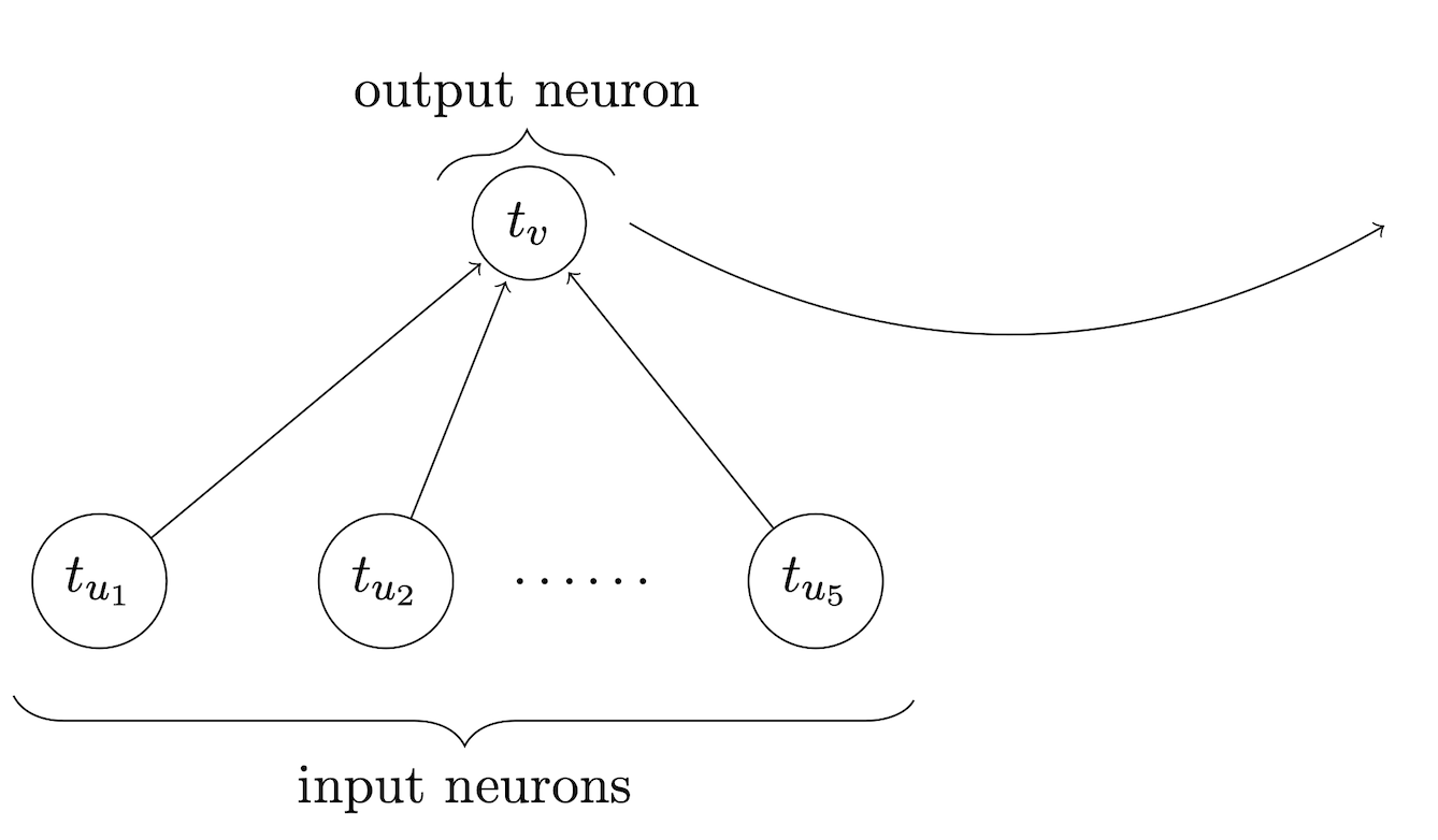
(a)

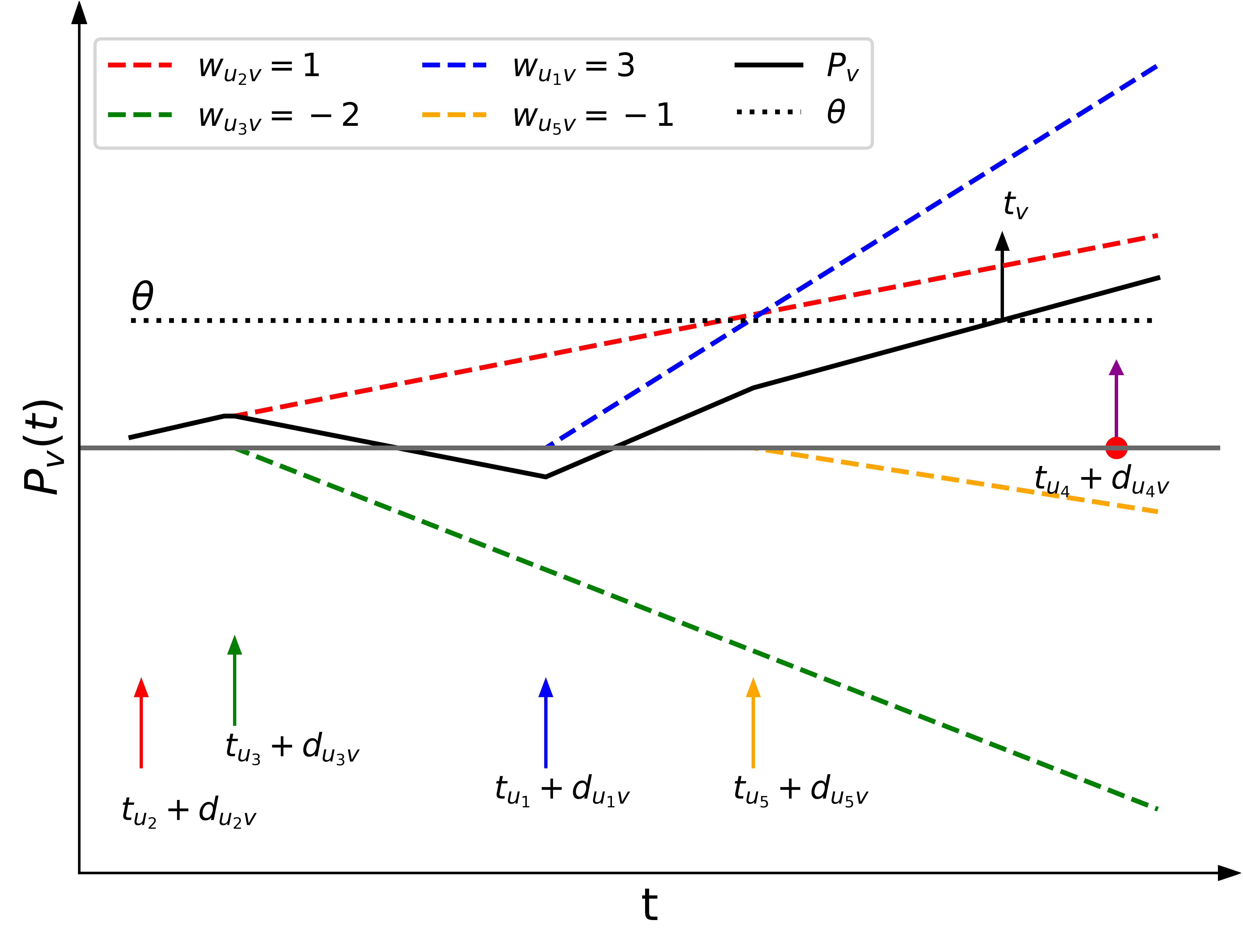
(b)

Figure 1: (a) A single layer spiking network with one output neuron $v$. Neuron $v$ receives inputs from five input neurons $u_{1},\dots,u_{5}$ that fire at times $t_{u_{1}},\dots,t_{u_{5}}$ respectively. (b) The trajectory in black shows the evolution of the membrane potential $P_{v}(t)$ of neuron $v$ as a result of spikes from input neurons that arrive at times $t_{u_{i}v}+d_{u_{i}v}$ (vertical arrows). Neurons $u_{1}$ and $u_{2}$ generate excitatory postsynaptic potentials with distinct strengths represented by $w_{u_{i}v}$, while neurons $u_{3}$ and $u_{5}$ produce inhibitory postsynaptic potentials with varying strengths (dashed lines). Neuron $v$ fires at time $t_{v}$ once $P_{v}(t_{v})=\theta$. The spike from neuron $u_{4}$ does not influence the firing time of $v$ since $t_{v}<t_{u_{4}}+d_{u_{4}v}$.

2.2 Input and output encoding

By restricting our framework of SNNs to acyclic graphs, we can arrange the underlying graph in layers and equivalently represent SNNs by a sequence of their parameters. This is analogous to the common representation of feedforward ANNs via a sequence of matrix-vector tuples ([3], [40]).

Definition 2.

Let $d,L\in\mathbb{N}$. A spiking neural network $\Phi$ with input dimension $d$ and $L$ layers associated to the acyclic graph $(V,E)$ is a sequence of matrix-matrix-vector tuples

$$\Phi=((W^{1},D^{1},\Theta^{1}),(W^{2},D^{2},\Theta^{2}),\dots,(W^{L},D^{L},\Theta^{L}))$$

where $N_{0}=d$ and $N_{1},N_{2},\dots,N_{L}\in\mathbb{N}$, and where each $W^{l}$ and each $D^{l}$ is an $N_{l-1}\times N_{l}$ matrix, and $\Theta^{l}\in\mathbb{R}_{+}^{N_{l}}$. $N_{0}$ is the input dimension and $N_{L}$ is the output dimension of the network. The matrix entry in $W^{l}_{uv}$ and $D^{l}_{uv}$ represents the weight and delay value associated with the synapse $(u,v)\in E$, and the entry $\Theta^{l}_{v}$ is the firing threshold associated with node $v$. We call $N(\Phi):=d+\sum_{j=1}^{L}N_{j}$ the number of neurons of the network $\Phi$, and $L(\Phi):=L$ denotes the number of layers of $\Phi$.

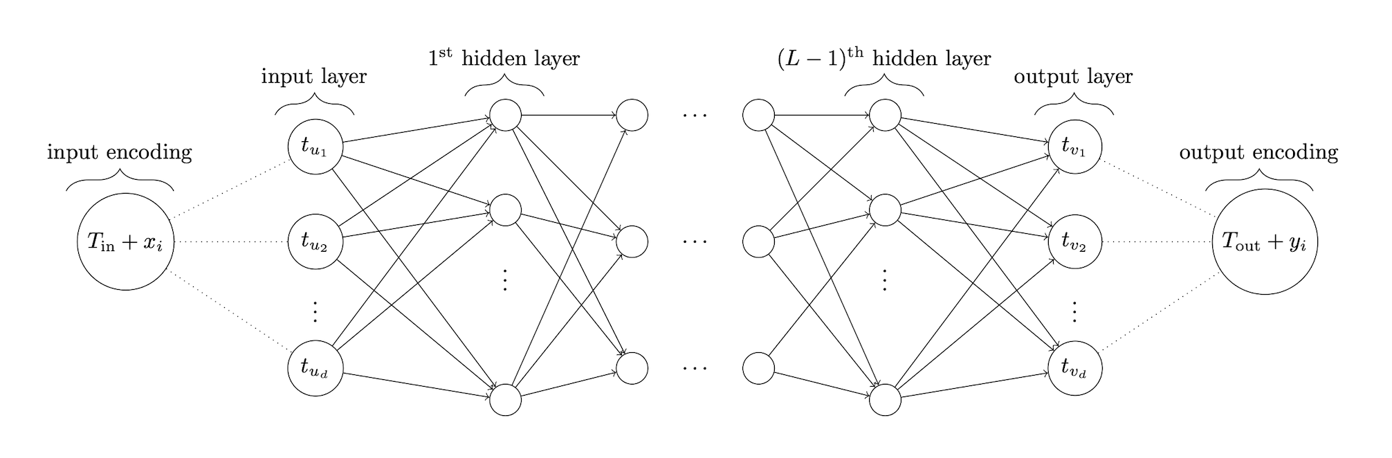
Figure 2: Computation graph associated with a spiking neural network $\Phi$ with input-output dimension $d$, width $d$ and $L-1$ hidden layers. The synapses in between the layers are labelled with synaptic weight matrices $W$ and delay matrices $D$. Each node in the network $\Phi$ is associated with a threshold parameter $\theta$. Analog input and output values are encoded in the firing time $t_{u_{i}}=T_{\text{in}}+x_{i}$ (respectively $t_{v_{i}}=T_{\text{out}}+y_{i}$) of a neuron.

Remark 3.

In an ANN, each layer performs some non-linear transformation on their inputs and then the information is propagated through the layers in a synchronized manner. However, in an SNN, information is transmitted through the network in the form of spikes. Spikes from neurons in layer $l-1$ influence the membrane potential of neurons in layer $l$ and ultimately trigger them to spike (according to the framework described in the previous paragraph). Hence, spikes are propagated through the network asynchronously since the firing times of the individual neurons vary.

The (typically analog) input information needs to be translated into the input firing times of the employed SNN, and similarly, the output firing times of the SNN need to be translated back to an appropriate target domain. We will refer to this process as input encoding and output decoding. In general, the applied encoding scheme certainly depends on the specific task at hand. For tasks that involve modelling complex time patterns or a sequence of events with multiple spikes, sophisticated encoding schemes may be required. However, we can formulate some guiding principles for establishing the encoding scheme. The firing times of input and output neurons should encode analog information in a consistent way so that different networks can be concatenated in a well-defined manner. This enables us to construct suitable subnetworks and combine them appropriately to solve more complex tasks. Second, our focus in this work lies on exploring the intrinsic capabilities of SNNs, rather than the specifics of the encoding scheme. In the extreme case, the encoding scheme might directly contain the solution to a problem, underscoring the need for a sufficiently simple and broadly applicable encoding scheme to avoid this. The potential power and suitability of different encoding schemes is a topic that warrants separate investigation on its own.

Remark 4.

Based on these considerations and our setting, we fix an appropriate encoding scheme. However, we will point out occasionally the effect of adjusting the scheme in certain ways. Analog input information is encoded in the firing times of the input neurons of an SNN $\Phi$ in the following manner: For any $x\in[a,b]^{d}$, $d\in\mathbb{N}$, $a,b\in\mathbb{R}$, we set the firing times of the input neurons $u_{1},\dots,u_{d}$ of $\Phi$ to $(t_{u_{1}},\dots,t_{u_{d}})^{T}=T_{\text{in}}+x$, where $T_{\text{in}}\in\mathbb{R}^{d}$ is some constant reference time, e.g., $T_{\text{in}}=(a,\dots,a)^{T}$. The bounded input domain ensures that an appropriate reference time can be fixed. The firing times of the non-input neurons of $\Phi$ are then determined based on (7). Finally, the firing times of the output neurons $v_{1},\dots,v_{n}$ encode the target $y\in\mathbb{R}^{n}$ via $(t_{v_{1}},\dots,t_{v_{d}})^{T}=T_{\text{out}}+y$, where $T_{\text{out}}\in\mathbb{R}^{n}$ is some constant reference time. For simplicity and with a slight abuse of notation, we will sometimes refer to $T_{\text{in}},T_{\text{out}}$ as one-dimensional objects, i.e., $T_{\text{in}},T_{\text{out}}\in\mathbb{R}$ which is justified as the corresponding vectors contain the same element in each dimension (see Figure 2). Additionally, note that the introduced encoding scheme translates analog information into input firing times in a continuous manner.

For the discussion ahead, we point out the difference between a network and the target function it realizes. A network is a structured set of weights, delays and thresholds as defined in Definition 2, and the target function it realizes is the result of the asynchronous propagation of spikes through the network.

Definition 3.

On $[a,b]^{d}$ with $a,b\in\mathbb{R}$, the realization of an SNN $\Phi$ with input reference time $T_{\text{in}}\in\mathbb{R}$ and $N_{L}\in\mathbb{N}$ output neurons $v_{1},\dots,v_{N_{L}}$ is defined as the map $\mathcal{R}_{\Phi}:\mathbb{R}^{d}\to\mathbb{R}^{N_{L}}$ such that

$$\mathcal{R}_{\Phi}(x)=(-T_{\text{out}}+t_{v_{1}},\dots,-T_{\text{out}}+t_{v_{N_{L}}})^{T},$$

where the firing times of the output neuron provide the realization $\mathcal{R}_{\Phi}(x)$ of $\Phi$ in temporal coding, i.e., $v_{1},\dots,v_{N_{L}}$ fire at time $(T_{\text{out}},\dots,T_{\text{out}})^{T}+\mathcal{R}_{\Phi}(x)$ for some fixed output reference time $T_{\text{out}}>T_{\text{in}}$.

Next, we give a corresponding definition of an ANN and its realization.

Definition 4.

Let $d,L\in\mathbb{N}$. An artificial neural network $\Psi$ consisting of $d$ input neurons and $L$ layers is a sequence of matrix-vector tuples

$$\Psi=((W^{1},B^{1}),(W^{2},B^{2}),\dots,(W^{L},B^{L}))$$

where $N_{0}=d$ and $N_{1},\dots,N_{L}\in\mathbb{N}$, and where each $W^{l}$ is an $N_{l-1}\times N_{l}$ matrix, and $B^{l}\in\mathbb{R}^{N_{l}}$. $N_{0}$ is the input dimension and $N_{L}$ is the output dimension of the network. We call $N(\Psi):=\sum_{j=0}^{L}N_{j}$ the number of neurons of the network $\Psi$, $L(\Psi):=L$ the number of layers of $\Psi$ and $N_{l}$ the width of $\Psi$ in layer $l$. The realization of $\Psi$ is defined as the map $\mathcal{R}_{\Psi}:\mathbb{R}^{N_{0}}\rightarrow\mathbb{R}^{N_{L}}$,

$$\mathcal{R}_{\Psi}(x)=y_{L},$$

where $y_{L}$ results from

$$y_{0} =x,$$

$$y_{l} =\sigma(W^{l}y_{l-1}+B^{l}),\>\>\text{for}\>l=1,\dots,L-1,$$

$$y_{L} =W^{L}y_{L-1}+B^{L},$$ (8)

where $\sigma:\mathbb{R}\to\mathbb{R}$ is acting component-wise and is called the activation function.

Remark 5.

From now on, we will always employ ReLU, i.e., $\sigma(x)=\max(0,x)$ as the activation function of an ANN. Finally, we assume that the realization is defined on some bounded domain $[a,b]^{d}\subset\mathbb{R}^{d}$.

One can perform basic actions on neural networks such as concatenation and parallelization to construct larger networks from existing ones. Adapting a general approach for ANNs as defined in ([3], [40]), we formally introduce the concatenation and parallelization of networks of spiking neurons in the Appendix A.1.

3 Main results

In the first part, we prove that SNNs generate Continuous Piecewise Linear (CPWL) mappings, followed by realizing a ReLU activation function using a two-layer SNN. Subsequently, we provide a general result that shows that SNNs can emulate the realization of any multi-layer ANN employing ReLU as an activation function. Lastly, we analyze the number of linear regions generated by SNNs and compare the arising pattern to the well-studied case of ReLU-ANNs. If not stated otherwise, the encoding scheme introduced in Remark 4 is applied and the results need to be understood with respect to this specific encoding.

3.1 Spiking neural networks realize continuous piecewise linear mapping

A broad class of ANNs based on a wide range of activation functions such as ReLU generate CPWL mappings [14], [13]. In other words, these ANNs partition the input domain into regions, the so-called linear regions, on which an affine function represents the neural network’s realization. We show that SNNs also express CPWL mappings under very general conditions. The proof of the statement can be found in the Appendix A.2.

Theorem 1.

Any SNN $\Phi$ realizes a CPWL function provided that the sum of synaptic weights of each neuron is positive and the encoding scheme is a CPWL function.

Remark 6.

Note that the encoding scheme introduced in Remark 4 is a CPWL mapping (in input as well as output encoding).

Remark 7.

The positivity of the sum of weights ensures that each neuron in the network emits a spike. In general, if this condition is not met by a neuron, then it does not fire for certain inputs. Therefore, the case may arise where an output neuron does not fire and the realization of the network is not well-defined. Via the given condition we prevent this behaviour. For a given SNN with an arbitrary but fixed input domain it is a sufficient but not necessary condition to guarantee that spikes are emitted by the the output neurons. Instead, one could also adapt the definition of the realization of an SNN, however, the CPWL property described in the theorem may be lost.

Despite the fact that ReLU is a very basic CPWL function, it is not straightforward to realize ReLU via SNNs; see Appendix A.3 for the proof.

Theorem 2.

Let $a<0<b$. There does not exist a one-layer SNN that realizes $\sigma(x)=\max(0,x)$ on $[a,b]$. However, $\sigma$ can be realized by a two-layer SNN on $[a,b]$.

Remark 8.

We note that the encoding scheme that converts the analog values into the time domain plays a crucial role. In the proof of the Theorem 2, an SNN is constructed that realizes $\sigma$ via the encoding scheme $T_{\text{in}}+\cdot$ and $T_{\text{out}}+\cdot$. At the same time, the encoding scheme $T_{\text{in}}-\cdot$ and $T_{\text{out}}-\cdot$ fails in the two-layer case. Moreover, utilizing an inconsistent input and output encoding enables us to construct a one-layer SNN that realizes $\sigma$. This shows that not only the network but also the applied encoding scheme is highly relevant. For details, we refer to Appendix A.3.

Remark 9.

Note that in a hypothetical real-world implementation, which certainly includes some noise, the constructed SNN that realizes ReLU is not necessarily robust with respect to input perturbation. Analyzing the behaviour and providing error estimations is an important future task.

3.2 Expressing ReLU-network realizations by spiking neural networks

In this subsection, we extend the realization of a ReLU neuron to the entire network, i.e., realize the output of any ReLU network using SNNs. The proof of the following statement can be found in the Appendix A.4.

Theorem 3.

Let $L,d\in\mathbb{N}$, $[a,b]^{d}\subset\mathbb{R}^{d}$ and let $\Psi$ be an arbitrary ANN of depth $L$ and fixed width $d$ employing a ReLU non-linearity, and having one-dimensional output. Then, there exists an SNN $\Phi$ with $N(\Phi)=N(\Psi)+L(2d+3)-(2d+2)$ and $L(\Phi)=3L-2$ that realizes $\mathcal{R}_{\Psi}$ on $[a,b]^{d}$.

Sketch of proof.

Any multi-layer ANN with ReLU activation is simply an alternating composition of affine-linear functions and a non-linear function represented by ReLU. To realize the mapping generated by some arbitrary ANN, it suffices to realize the composition of affine-linear functions and the ReLU non-linearity and then extend the construction to the whole network using concatenation and parallelization operations. ∎

Remark 10.

The aforementioned result can be generalized to ANNs with varying widths that employ any type of piecewise linear activation function.

Remark 11.

In this work, the complexity of neural networks is assessed in terms of the number of computational units and layers. However, the complexity of an SNN can be captured in different ways as well. For instance, the total number of spikes emitted in an SNN is related to its energy consumption (since emitting spikes consumes energy). Hence, the minimum number of spikes to realize a given function class may be a reasonable complexity measure for an SNN (with regard to energy efficiency). Further research in this direction is necessary to evaluate the complexity of SNNs via different measures with their benefits and drawbacks.

3.3 Equivalence of approximation

It is well known that ReLU-ANNs not only realize CPWL mappings but that every CPWL function in $\mathbb{R}^{d}$ can be represented by ReLU-ANNs if there are no restrictions placed on the number of parameters or the depth of the network [2], [12]. Therefore, ReLU-ANNs can represent any SNN with a CPWL encoding scheme. On the other hand, our results also imply that SNNs can represent every ReLU-ANN and thereby every CPWL function in $\mathbb{R}^{d}$. The key difference in the realization of arbitrary CPWL mappings is the necessary size and complexity of the respective ANN and SNN.

Recall that realizing the ReLU activation via SNNs required more computational units than the corresponding ANN (see Theorem 3). Conversely, we demonstrate using a toy example that SNNs can realize certain CPWL functions with fewer number of computational units and layers compared to ReLU-based ANNs.

Example 1.

For $\theta>0$, $[a,b]\subset\mathbb{R}$, consider the CPWL function $f:[a,b]\to\mathbb{R}$ given by

$$f(x)=\begin{cases}x,&x\leq-\theta\\ \frac{x-\theta}{2},&-\theta<x<\theta\\ 0,&\,x\geq\theta\end{cases}\quad=-\frac{1}{2}\sigma(-x-\theta)-\frac{1}{2}\sigma(-x+\theta),$$ (9)

where $\sigma$ is the ReLU activation. A one-layer SNN with one output unit and two input units can realize $f$. However, to realize $f$, any ReLU-ANN requires at least two layers and four computational units; see Appendix A.5 for the proof.

These observations illustrate that the computational structure of SNNs differs significantly from that of ReLU-ANNs. While neither model is clearly beneficial in terms of network complexity to express all CPWL functions, each model has distinct advantages and disadvantages. To gain a better understanding of this divergent behaviour, in the next section, we study the number of linear regions that SNNs generate.

3.4 Number of linear regions

The number of linear regions can be seen as a measure for the flexibility and expressivity of the corresponding CPWL function. Similarly, we can measure the expressivity of an ANN by the number of linear regions of its realization. The connection of the depth, width, and activation function of a neural network to the maximum number of its linear regions is well-established, e.g., with increasing depth the number of linear regions can grow exponentially in the number of parameters of an ANN ([38], [2], [17]). This property offers one possible explanation for why deep networks tend to outperform shallow networks in expressing complex functions. Can we observe a similar behaviour for SNNs?

To that end, we first analyze the properties of a spiking neuron. For the proof, we refer to Appendix A.2.

Theorem 4.

Let $\Phi$ be a one-layer SNN with a single output neuron $v$ and $d$ input neurons $u_{1},\dots,u_{d}$ such that $\sum_{i=1}^{d}w_{u_{i}v}>0$. Then $\Phi$ partitions the input domain into at most $2^{d}-1$ linear regions. In particular, for a sufficiently large input domain, the maximal number of linear regions is attained if and only if all synaptic weights are positive.

Remark 12.

By examining the parameters of $\Phi$, one can assess the number of linear regions into which the input domain is divided by $\Phi$. For instance, if a single input neuron $u_{j}$ causes the firing of $v$, then the corresponding synaptic weight $w_{u_{j}v}$ is necessarily positive. Thus, if $w_{u_{j}v}\leq 0$, then $u_{j}$ could not have caused the firing of $v$ and $\Phi$ can under no circumstances achieve the maximal number of linear regions. Similarly, one can derive via (7) that any subset of input neurons {$u_{j_{1}},\dots,u_{j_{k}}\}$ with $\sum_{i}w_{u_{j_{i}}v}\leq 0$ did not cause a firing of $v$. The condition $\sum_{i=1}^{d}w_{u_{i}v}>0$ simply ensures that the notion of linear region is applicable. Otherwise, the input domain is still partitioned into polytopes by the SNN but there exists a region where the realization of the network is not well-defined (see Remark 7). Finally, to ensure that the linear region corresponding to a subset of input neurons with a positive sum of weights is actually realized, the input domain simply needs to be chosen suitably large.

Remark 13.

One-layer ReLU-ANNs and one-layer SNNs with one output neuron both partition the input domain into linear regions. Nevertheless, the differences are noteworthy. A one-layer ReLU-ANN will partition the input domain into at most two linear regions, independent of the dimension of the input. In contrast, for a one-layer SNN the maximum number of linear regions scales exponentially in the input dimension. One may argue that the distinct behaviour arises due to the fact that the ‘non-linearity’ in the SNN is directly applied on the input, whereas the non-linearity in the ANN is applied on the single output neuron. By shifting the non-linearity and applying it instead on the input, the ANN would exhibit the same exponential scaling of the linear regions as the SNN. However, this change would not reflect the intrinsic capabilities of the ANN since it has rather detrimental effect on the expressivity and, in particular, the partitioning of the input domain is fixed and independent of the parameters of the ANN. In contrast, for SNNs one can also explicitly compute the boundaries of the linear regions. This is exemplarily demonstrated for a two-dimensional input space in Appendix A.2. It turns out that only specific hyperplanes are eligible as boundaries of the linear region in this simple scenario. Hence, the flexibility of the SNN model to generate arbitrary linear regions is to a certain extent limited, albeit not entirely restricted as in the adjusted ANN.

Although we established interesting differences in the structure of computations between SNNs and ANNs, many questions remain open. In particular, the effect of depth in SNNs needs further consideration. The full power of ANN comes into play with large numbers of layers. Our result in Theorem 4 suggests that a shallow SNN can be as expressive as a deep ReLU network in terms of the number of linear regions required to express certain types of CPWL functions. In ([14]; Lemma 3), the authors showed that a deep neural network employing any piecewise linear activation function cannot span all CPWL functions with the number of linear regions scaling exponentially in the number of parameters of the network. Studying these types of functions and identifying (or excluding) similar behaviour for SNNs requires a deeper analysis of the capabilities of SNNs, providing valuable insights into their computational power. This aspect is left for future investigation.

4 Related work

The inherently complex dynamics of spiking neurons complicate the analysis of computations carried out by an SNN. In this section, we mention the most relevant results that investigate their computational or expressive power. One of the central results in this direction is the Universal Approximation Theorem for SNNs [31]. The author showed the existence of SNNs that approximates arbitrary feedforward ANNs employing sigmoidal activation function and thus, approximating any continuous function. The result is based on temporal coding by single spikes and under the presence of some additional assumptions on the response and threshold functions. In contrast, we show that an SNN can realize the output of an arbitrary ANN with CPWL activation and further specify the size of the network to achieve the associated realization, which has not been previously demonstrated. Moreover, we also study the expressivity of SNNs in terms of the number of linear regions and provide new insights on realizations generated by SNNs. [10] shows that continuous functions can be approximated to arbitrary precision using SNNs in temporal coding. In another direction, the author in [32] constructed SNNs that simulate arbitrary threshold circuits, Turing machines and a certain type of random access machines with real-valued inputs.

In [62], the authors delve into the theoretical exploration of self-connection spike neural networks (scSNNs), analyzing their approximation capabilities and computational efficiency. The theoretical findings demonstrate that scSNNs, when equipped with self-connections, can effectively approximate discrete dynamical systems with a polynomial number of parameters and within polynomial time complexities. Our approach centers on precise spike timing, while theirs hinges on firing rates and includes a distinct model featuring self-connections, further setting their approach apart from ours. The study by [55] presents convergence theory that rigorously establishes the convergence of firing rates to solutions corresponding to LASSO problems in the Locally Competitive Algorithms framework.

Another line of research focuses on converting (trained) ANNs, in particular with ReLU activation, into equivalent SNNs and, thereby avoiding or facilitating the training process of SNNs. This has been studied for various encoding schemes, spike patterns and spiking neuron models ([49], [52], [26], [45], [44], [60], [43], [63], [61]). By introducing a general algorithmic conversion from ANNs to SNNs, one also establishes approximation and/or emulation capabilities of SNNs in the considered setting. Most related to our analysis of the expressivity of SNNs are the results in [52]. The authors define a one-to-one neuron mapping that converts a trained ReLU neural network to a corresponding SNN consisting of integrate and fire neurons by a non-linear transformation of parameters. This is done under the assumption of having access to a trained ReLU network, weights and biases of the trained model and the input data on which the model was trained. We point out that the underlying idea of representing information in terms of spike time and aptly choosing the parameters of an SNN model such that the output is encoded in the firing time is similar to ours. However, significant distinctions exist between our approach and theirs, particularly in terms of the chosen model, objectives, and methodology. Our choice of the model is driven by our intention to better understand expressivity outcomes. In terms of methodology, we introduce an auxiliary neuron to ensure the firing of neurons even when a corresponding ReLU neuron exhibits zero activity. This diverges from their approach, which employs external current and a special parameter to achieve similar outcomes. Moreover, our work involves a fixed threshold for neuron firing, whereas their model incorporates a threshold that varies with time. Lastly, we study the differences in expressivity and structure of computations between ANNs and SNNs, whereas in [52], only the general conversion of ANNs to SNNs is examined and not vice versa.

Finally, we would like to mention that a connection between SNNs and piecewise linear functions was already noted in [37]. The author shows that a spiking network consisting of non-leaky integrate and fire neurons, employing exponentially decaying synaptic current kernels and temporal coding, exhibits a piecewise linear input-output relation after a transformation of the time variable. This piecewise relation is continuous unless small perturbations influences the spiking behaviour, specifically concerning whether the neuron fires or remains inactive.

5 Discussion

The central aim of this paper is to study and compare the expressive power of SNNs and ANNs employing any piecewise linear activation function. In an ANN, information is propagated across the network in a synchronized manner. In contrast, in SNNs, spikes are only emitted once a subset of neurons in the previous layer triggers a spike in a neuron in the subsequent layer. Hence, the imperative role of time in biological neural systems accounts for differences in computation between SNNs and ANNs. We show that a one-layer SNN with one output neuron can partition the input domain into an exponential number of linear regions with respect to the input dimension. The exact number of linear regions depends on the parameters of the network. Our expressivity result in Theorem 3 implies that SNNs can essentially approximate any function with the same accuracy and (asymptotic) complexity bounds as (deep) ANNs employing a piecewise linear activation function, given the response function satisfies some basic assumptions. Rather than approximating some function space by emulating a known construction for ReLU networks, one could also achieve optimal approximations by leveraging the intrinsic capabilities of SNNs instead. The findings in Theorem 4 indicate that the latter approach may indeed be beneficial in terms of the complexity of the architecture in certain circumstances. However, we point out that finding optimal architectures for approximating different classes of functions is not the focal point of our work. The significance of our results lies in investigating theoretically the approximation and expressivity capabilities of SNNs, highlighting their potential as an alternative computational model for complex tasks. The insights obtained from this work can further aid in designing architectures that can be implemented on neuromorphic hardware for energy-efficient applications.

Extending the model of a spiking neuron by incorporating, e.g., multiple spikes of a neuron, may yield improvements on our results. However, by increasing the complexity of the model the analysis also tends to be more elaborate. In the aforementioned case of multiple spikes the threshold function becomes important so that additional complexity when approximating some target function is introduced since one would have to consider the coupled effect of response and threshold functions. Similarly, the choice of the response function and the frequency of neuron firings will surely influence the approximation results and we leave this for future work.

Limitations

In theory, we prove that SNNs are as expressive as ReLU-ANNs. However, achieving similar results in practice heavily relies on the effectiveness of the training algorithms employed. The implementation of efficient learning algorithms with weights, delays and thresholds as programmable parameters is left for future work. However, there already exists training algorithms such as the SpikeProp algorithm [5], [51], which consider the same programmable parameters as our model and may be a reasonable starting point for future implementations. In this work, our choice of model resides on theoretical considerations and not on practical considerations regarding implementation. However, there might be other models of spiking neurons that are more apt for implementation purposes — see e.g. [52] and [9]. Furthermore, in reality, due to the ubiquitous sources of noise in the spiking neurons, the firing activity of a neuron is not deterministic. For mathematical simplicity, we perform our analysis in a noise-free case. Generalizing to the case of noisy spiking neurons is important (for instance with respect to the aforementioned implementation in noisy environments) and may lead to further insights in the model.

Appendix A Appendix

Outline

We start by introducing the spiking network calculus in Section A.1 to compose and parallelize different networks. In Section A.2, we show that SNNs output CPWL functions and establish a relation between the input dimension of an SNN and the number of linear regions. The proof of Theorem 2 is given in Section A.3. Finally, in Section A.4, we prove that an SNN can realize the output of any ReLU network.

A.1 Spiking neural network calculus

It can be observed from Remark 4 that both inputs and outputs of SNNs are encoded in a unified format. This characteristic is crucial for concatenating/parallelizing two spiking network architectures that further enable us to attain compositions/parallelizations of network realizations.

We operate in the following setting: Let $L_{1}$, $L_{2},d_{1},d_{2},d_{1}^{\prime},d_{2}^{\prime}\in\mathbb{N}$. Consider two SNNs $\Phi_{1}$, $\Phi_{2}$ given by

$$\Phi_{i}=((W_{1}^{i},D_{1}^{i},\Theta_{1}^{i}),\dots,(W_{L_{i}}^{i},D_{L_{i}}^{i},\Theta_{L_{i}}^{i})),\quad i=1,2,$$

with input domains $[a_{1},b_{1}]^{d_{1}}\subset\mathbb{R}^{d_{1}}$, $[a_{2},b_{2}]^{d_{2}}\subset\mathbb{R}^{d_{2}}$ and output dimension $d_{1}^{\prime},d_{2}^{\prime}$, respectively. Denote the input neurons by $u_{1},\dots,u_{d_{i}}$ with respective firing times $t^{i}_{u_{j}}$ and the output neurons by $v_{1},\dots,v_{d^{\prime}_{i}}$ with respective firing times $t^{i}_{v_{j}}$ for $i=1,2$. By Remark 4, we can express the firing times of the input neurons as

$$t_{u}^{1}(x):=(t^{1}_{u_{1}},\dots,t^{1}_{u_{d_{1}}})^{T} =T^{1}_{\text{in}}+x\quad\text{ for }x\in[a_{1},b_{1}]^{d_{1}},$$

$$t_{u}^{2}(x):=(t^{2}_{u_{1}},\dots,t^{2}_{u_{d_{2}}})^{T} =T^{2}_{\text{in}}+x\quad\text{ for }x\in[a_{2},b_{2}]^{d_{2}}$$ (10)

and, by Definition 3, the realization of the networks as

$$\mathcal{R}_{\Phi_{1}}(x) =-T^{1}_{\text{out}}+t^{1}_{v}(t^{1}_{u}(x)):=-T^{1}_{\text{out}}+(t^{1}_{v_{1}},\dots,t^{1}_{v_{d_{1}^{\prime}}})^{T}\quad\text{ for }x\in[a_{1},b_{1}]^{d_{1}},$$

$$\mathcal{R}_{\Phi_{2}}(x) =-T^{2}_{\text{out}}+t^{2}_{v}(t^{2}_{u}(x)):=-T^{2}_{\text{out}}+(t^{2}_{v_{1}},\dots,t^{2}_{v_{d_{2}^{\prime}}})^{T}\quad\text{ for }x\in[a_{2},b_{2}]^{d_{2}}$$ (11)

for some constants $T^{1}_{\text{in}}\in\mathbb{R}^{d_{1}}$, $T^{2}_{\text{in}}\in\mathbb{R}^{d_{2}}$, $T^{1}_{\text{out}}\in\mathbb{R}^{d^{\prime}_{1}}$, $T^{2}_{\text{out}}\in\mathbb{R}^{d^{\prime}_{2}}$.

We define the concatenation of the two networks in the following way.

Definition 5.

(Concatenation) Let $\Phi_{1}$ and $\Phi_{2}$ be such that the input layer of $\Phi_{1}$ has the same dimension as the output layer of $\Phi_{2}$, i.e., $d_{2}^{\prime}=d_{1}$. Then, the concatenation of $\Phi_{1}$ and $\Phi_{2}$, denoted as $\Phi_{1}\bullet\Phi_{2}$, represents the $(L_{1}+L_{2})$-layer network

$$\Phi_{1}\bullet\Phi_{2}:=((W_{1}^{2},D_{1}^{2},\Theta_{1}^{2}),\dots,(W_{L_{2}}^{2},D_{L_{2}}^{2},\Theta_{L_{2}}^{2}),(W_{1}^{1},D_{1}^{1},\Theta_{1}^{1}),\dots,(W_{L_{1}}^{1},D_{L_{1}}^{1},\Theta_{L_{1}}^{1})).$$

Lemma 1.

Let $d_{2}^{\prime}=d_{1}$ and fix $T_{\text{in}}=T^{2}_{\text{in}}$ and $T_{\text{out}}=T^{1}_{\text{out}}$. If $T^{2}_{\text{out}}=T^{1}_{\text{in}}$ and $\mathcal{R}_{\Phi_{2}}([a_{2},b_{2}]^{d_{2}})\subset[a_{1},b_{1}]^{d_{1}}$, then

$$\mathcal{R}_{\Phi_{1}\bullet\Phi_{2}}(x)=\mathcal{R}_{\Phi_{1}}(\mathcal{R}_{\Phi_{2}}(x))\quad\text{for all}\>\>x\in[a,b]^{d_{2}}$$

with respect to the reference times $T_{\text{in}},T_{\text{out}}$. Moreover, $\Phi_{1}\bullet\Phi_{2}$ is composed of $N(\Phi_{1})+N(\Phi_{2})-d_{1}$ computational units.

Proof.

It is straightforward to verify via the construction that the network $\Phi_{1}\bullet\Phi_{2}$ is composed of $N(\Phi_{1})+N(\Phi_{2})-d_{1}$ computational units. Moreover, under the given assumptions $\mathcal{R}_{\Phi_{1}}\circ\mathcal{R}_{\Phi_{2}}$ is well-defined so that (A.1) and (A.1) imply

$$\mathcal{R}_{\Phi_{1}\bullet\Phi_{2}}(x) =-T_{\text{out}}+t_{v}^{1}(t_{v}^{2}(T_{\text{in}}+x))=-T^{1}_{\text{out}}+t_{v}^{1}(t_{v}^{2}(T^{2}_{\text{in}}+x))=-T^{1}_{\text{out}}+t^{1}_{v}(t^{2}_{v}(t^{2}_{u}(x)))$$

$$=-T^{1}_{\text{out}}+t^{1}_{v}(T^{2}_{\text{out}}+\mathcal{R}_{\Phi_{2}}(x))=-T^{1}_{\text{out}}+t^{1}_{v}(T^{1}_{\text{in}}+\mathcal{R}_{\Phi_{2}}(x))$$

$$=-T^{1}_{\text{out}}+t^{1}_{v}(t^{1}_{u}(\mathcal{R}_{\Phi_{2}}(x)))=\mathcal{R}_{\Phi_{1}}(\mathcal{R}_{\Phi_{2}}(x))\quad\text{ for }x\in[a_{2},b_{2}]^{d_{2}}.$$

∎

In addition to concatenating networks, we also perform parallelization operation on SNNs.

Definition 6.

(Parallelization) Let $\Phi_{1}$ and $\Phi_{2}$ be such that they have the same depth and input dimension, i.e., $L_{1}=L_{2}=:L$ and $d_{1}=d_{2}=:d$. Then, the parallelization of $\Phi_{1}$ and $\Phi_{2}$, denoted as $P(\Phi_{1},\Phi_{2})$, represents the $L$-layer network with $d$-dimensional input

$$P(\Phi_{1},\Phi_{2}):=((\tilde{W}_{1},\tilde{D}_{1},\tilde{\Theta}_{1}),\dots,(\tilde{W}_{L},\tilde{D}_{L},\tilde{\Theta}_{L})),$$

where

$$\tilde{W}_{1}=\begin{pmatrix}W_{1}^{1}&W_{1}^{2}\\[3.0pt] \end{pmatrix},\quad\tilde{D}_{1}=\begin{pmatrix}D_{1}^{1}&D_{1}^{2}\\[3.0pt] \end{pmatrix},\quad\tilde{\Theta}_{1}=\begin{pmatrix}\Theta_{1}^{1}\\[3.0pt] \Theta_{1}^{2}\\ \end{pmatrix}$$

and

$$\tilde{W}_{l}=\begin{pmatrix}W_{l}^{1}&0\\ 0&W_{l}^{2}\\ \end{pmatrix},\quad\tilde{D}_{l}=\begin{pmatrix}D_{l}^{1}&0\\ 0&D_{l}^{2}\\ \end{pmatrix},\quad\tilde{\Theta}_{l}=\begin{pmatrix}\Theta_{l}^{1}\\[2.0pt] \Theta_{l}^{2}\\ \end{pmatrix},\quad\text{for}\>\>1<l\leq L.$$

Lemma 2.

Let $d:=d_{2}=d_{1}$ and fix $T_{\text{in}}:=T^{1}_{\text{in}}$, $T_{\text{out}}:=(T^{1}_{\text{out}},T^{2}_{\text{out}})$, $a:=a_{1}$ and $b:=b_{1}$. If $T^{2}_{\text{in}}=T^{1}_{\text{in}}$, $T^{2}_{\text{out}}=T^{1}_{\text{out}}$ and $a_{1}=a_{2}$, $b_{1}=b_{2}$, then

$$\mathcal{R}_{P(\Phi_{1},\Phi_{2})}(x)=(\mathcal{R}_{\Phi_{1}}(x),\mathcal{R}_{\Phi_{2}}(x))\quad\text{ for }x\in[a,b]^{d}$$

with respect to the reference times $T_{\text{in}},T_{\text{out}}$. Moreover, $P(\Phi_{1},\Phi_{2})$ is composed of $N(\Phi_{1})+N(\Phi_{2})-d$ computational units.

Proof.

The number of computational units is an immediate consequence of the construction. Since the input domains of $\Phi_{1}$ and $\Phi_{2}$ agree, (A.1) and (A.1) show that

$$\mathcal{R}_{P(\Phi_{1},\Phi_{2})}(x) =-T_{\text{out}}+(t_{v}^{1}(T_{\text{in}}+x),t_{v}^{2}(T_{\text{in}}+x))=(-T^{1}_{\text{out}}+t_{v}^{1}(T^{1}_{\text{in}}+x),-T^{2}_{\text{out}}+t_{v}^{2}(T^{2}_{\text{in}}+x))$$

$$=(-T^{1}_{\text{out}}+t_{v}^{1}(t^{1}_{u}(x)),-T^{2}_{\text{out}}+t_{v}^{2}(t_{u}^{2}(x)))=(\mathcal{R}_{\Phi_{1}}(x),\mathcal{R}_{\Phi_{2}}(x))\quad\text{ for }x\in[a,b]^{d}.$$

∎

Remark 14.

Note that parallelization and concatenation can be straightforwardly extended (recursively) to a finite number of networks. Additionally, more general forms of parallelization and concatenations of networks, e.g., parallelization of networks with different depths, can be established. However, for the constructions presented in this work, the introduced notions suffice.

A.2 Realizations of spiking neural networks

In this section, we analyze the realization of an SNN. We show that a spiking neuron with arbitrarily many input neurons generates a CPWL mapping and establish a correspondence between the input dimension of the spiking neurons and the number of linear regions of the associated realization. For simplicity, we perform the analysis without employing an encoding scheme of analog values in the time domain via the firing time of the input neurons. However, it is straightforward to incorporate the encoding into the analysis. Moreover, since we show that the firing time of a spiking neuron is a CPWL function on the input domain, it immediately follows that any spiking neuron with a CPWL encoding scheme, e.g., as defined in Remark 4, realizes a CPWL mapping. The final step is to extend the analysis from a single spiking neuron to a network of spiking neurons.

A.2.1 Spiking neuron with two inputs

First, we provide a simple toy example to demonstrate the dynamics of a spiking neuron. Let $v$ be a spiking neuron with two input neurons $u_{1},u_{2}$. Denote the associated weights and delays by $w_{u_{i}v}\in\mathbb{R}$ and $d_{u_{i}v}\geq 0$, respectively, and the threshold of $v$ by $\theta_{v}>0$. A spike emitted from $v$ could then be caused by either $u_{1}$ or $u_{2}$ or a combination of both. Each possibility corresponds to a linear region in the input space $\mathbb{R}^{2}$. We consider each case separately under the assumption that $\delta$ in (3) is arbitrarily large and we discuss the implications of this assumption in more detail after presenting the different cases.

Case 1: $u_{1}$ causes $v$ to spike before a potential effect from $u_{2}$ reaches $v$. Note that this can only happen if $w_{u_{1}v}>0$ and

$$t_{u_{2}}+d_{u_{2}v}\geq t_{v}=\frac{\theta_{v}}{w_{u_{1}v}}+t_{u_{1}}+d_{u_{1}v},$$

where we applied (6) and (7), and $t_{z}$ represents the firing time of a neuron $z$. Solving for $t_{u_{2}}$ leads to

$$t_{u_{2}}\geq\frac{\theta_{v}}{w_{u_{1}v}}+t_{u_{1}}+d_{u_{1}v}-d_{u_{2}v}.$$

Case 2: An analogous calculation shows that

$$t_{u_{2}}\leq-\frac{\theta_{v}}{w_{u_{2}v}}+t_{u_{1}}+d_{u_{1}v}-d_{u_{2}v},$$

whenever $u_{2}$ causes $v$ to spike before a potential effect from $u_{1}$ reaches $v$.

Case 3: The remaining possibility is that spikes from $u_{1}$ and $u_{2}$ influence the firing time of $v$. Then, the following needs to hold: $w_{u_{1}v}+w_{u_{2}v}>0$ and

$$t_{u_{1}}+d_{u_{1}v} <t_{v}=\frac{\theta_{v}}{w_{u_{1}v}+w_{u_{2}v}}+\sum_{i}\frac{w_{u_{i}v}}{w_{u_{1}v}+w_{u_{2}v}}(t_{u_{i}}+d_{u_{i}v})\quad\text{ and }$$

$$t_{u_{2}}+d_{u_{2}v} <t_{v}=\frac{\theta_{v}}{w_{u_{1}v}+w_{u_{2}v}}+\sum_{i}\frac{w_{u_{i}v}}{w_{u_{1}v}+w_{u_{2}v}}(t_{u_{i}}+d_{u_{i}v}).$$

This yields

$$t_{u_{2}} \begin{cases}>-\frac{\theta_{v}}{w_{u_{2}v}}+t_{u_{1}}+d_{u_{1}v}-d_{u_{2}v},&\text{ if }\frac{w_{u_{2}v}}{w_{u_{1}v}+w_{u_{2}v}}>0\\[7.0pt] <-\frac{\theta_{v}}{w_{u_{2}v}}+t_{u_{1}}+d_{u_{1}v}-d_{u_{2}v},&\text{ if }\frac{w_{u_{2}v}}{w_{u_{1}v}+w_{u_{2}v}}<0\end{cases},$$

respectively

$$t_{u_{2}} \begin{cases}<\frac{\theta_{v}}{w_{u_{1}v}}+t_{u_{1}}+d_{u_{1}v}-d_{u_{2}v},&\text{ if }\frac{w_{u_{1}v}}{w_{u_{1}v}+w_{u_{2}v}}>0\\[7.0pt] >\frac{\theta_{v}}{w_{u_{1}v}}+t_{u_{1}}+d_{u_{1}v}-d_{u_{2}v},&\text{ if }\frac{w_{u_{1}v}}{w_{u_{1}v}+w_{u_{2}v}}<0\end{cases}.$$

Example 2.

In a simple setting with $\theta_{v}=w_{u_{i}v}=d_{u_{2}v}=1$ and $d_{u_{1}v}=2$, the above considerations imply the following firing time of $v$ on the corresponding linear regions (see Figure 3):

$$t_{v}=\begin{cases}t_{u_{1}}+3,&\text{ if }t_{u_{2}}\geq t_{u_{1}}+2\\[4.0pt] t_{u_{2}}+2,&\text{ if }t_{u_{2}}\leq t_{u_{1}}\\[4.0pt] \frac{1}{2}(t_{u_{1}}+t_{u_{2}})+2,&\text{ if }t_{u_{1}}<t_{u_{2}}<t_{u_{1}}+2\end{cases}.$$

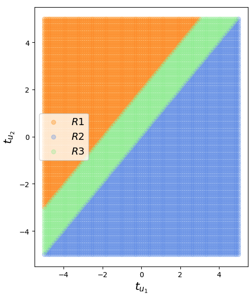
(a)

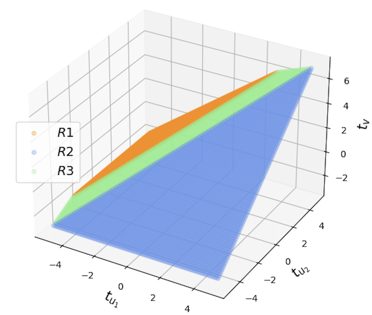
(b)

Figure 3: Illustration of Example 2. It shows that the output firing time $t_{v}(t_{u_{1}},t_{u_{2}})$ as a function of inputs $t_{u_{1}},t_{u_{2}}$ is a CPWL mapping. (a) An illustration of the partitioning of the input space into three different regions. (b) Each region is associated with an affine-linear mapping.

Already this simple setting with two-dimensional inputs provides crucial insights. The actual number of linear regions in the input domain corresponds to the parameter of the spiking neuron $v$. In particular, the maximum number of linear regions, i.e. three, can only occur if both weights $w_{u_{i}v}$ are positive. Similarly, $v$ does not fire at all if both weights are non-positive. The exact number of linear regions depends on the sign and magnitude of the weights. Furthermore, note that the linear regions are described by hyperplanes of the form

$$t_{u_{2}}\lesseqgtr t_{u_{1}}+C_{p,u},$$ (12)

where $C_{p,u}$ is a constant depending on the parameter $p$ corresponding to $v$, i.e., threshold, delays and weights, and the actual input neuron(s) causing $v$ to spike. Hence, $p$ has only a limited effect on the boundary of a linear region; depending on their exact value, the parameter only introduces an additive constant shift.

Remark 15.

Dropping the assumption that $\delta$ is arbitrarily large in (3) yields an evolved model which is also biologically more realistic. The magnitude of $\delta$ describes the duration in which an incoming spike influences the membrane potential of a neuron. By setting $\delta$ arbitrarily large, we generally consider an incoming spike to have a lasting effect on the membrane potential. Specifying a fixed $\delta$ increases the importance of the timing of the individual spikes as well as the choice of the parameter. For instance, inputs from certain regions in the input domain may not trigger a spike any more since the combined effect of multiple delayed incoming spikes is neglected. An in-depth analysis of the influence of $\delta$ is left as future work and we continue our analysis under the assumption that $\delta$ is arbitrarily large.

A.2.2 Spiking neuron with arbitrarily many inputs

A significant observation in the two-dimensional case is that the firing time $t_{v}(t_{u_{1}},t_{u_{2}})$ as a function of the input $t_{u_{1}},t_{u_{2}}$ is a CPWL mapping. Indeed, each linear region is associated with an affine linear mapping and crucially these affine mappings agree at the breakpoints. This intuitively makes sense since a breakpoint marks the event when the effect of an additional neuron on the firing time of $v$ needs to be taken into consideration or, equivalently, a neuron does not contribute to the firing of $v$ any more. However, in both circumstances, the effective contribution of this specific neuron is zero (and the contribution of the other neuron remains unchanged) at the breakpoint so that the crossing of a breakpoint and the associated change of a linear region does not result in a discontinuity. We can straightforwardly extend the insights of the two-dimensional to a $d$-dimensional input domain.

Formally, the class of CPWL functions describes functions that are globally continuous and locally linear on each polytope in a given finite decomposition of $\mathbb{R}^{d}$ into polytopes. We refer to the polytopes as linear regions. First, we assess the number of regions the input domain is partitioned by a spiking neuron.

Proposition 1.

Let $v$ be a spiking neuron with $d$ input neurons $u_{1},\dots,u_{d}$. Then $\mathbb{R}^{d}$ is partitioned by $v$ into at most $2^{d}-1$ regions.

Proof.

The maximum number of regions directly corresponds to $E(\mathbf{t}_{U})$ defined in (7). Recall that $E(\mathbf{t}_{U})$ identifies the presynaptic neurons that based on their firing times $\mathbf{t}_{U}=(t_{u_{i}})_{i=1}^{d}$ triggered the firing of $v$ at time $t_{v}$. Therefore, each region in the input domain is associated to a subset of input neurons that is responsible for the firing of $v$ on this specific domain. Hence, the number of regions is bounded by the number of non-empty subsets of $\{u_{1},\dots,u_{d}\}$, i.e., $2^{d}-1$. ∎

Remark 16.

Observe that any subset of input neurons causes a spike in $v$ if and only if the sum of their weights is positive. Otherwise, the corresponding input region either does not exist or inputs from the corresponding region do not trigger a spike in $v$ since they can not increase the potential $P_{v}(t)$ as their net contribution is negative, i.e., the potential does not reach the threshold $\theta_{v}$. Hence, the maximal number of regions is attained if and only if all weights are positive and thereby the sum of weights of any subset of input neurons is positive as well.

Remark 17.

The observations with regard to the parameter $\delta$ in Remark 15 directly transfer from the two- to the $d$-dimensional setting.

Next, we show that a spiking neuron generates a CPWL mapping.

Theorem 5.

Let $v$ be a spiking neuron with $d$ input neurons $u_{1},\dots,u_{d}$. The firing time $t_{v}(t_{u_{1}},\dots,t_{u_{d}})$ as a function of the firing times $t_{u_{1}},\dots,t_{u_{d}}$ is a CPWL mapping provided that $\sum_{i=1}^{d}w_{u_{i}v}>0$, where $w_{u_{i}v}\in\mathbb{R}$ is the synaptic weight between $u_{i}$ and $v$.

Proof.

The condition $\sum_{i=1}w_{u_{i}v}>0$ simply ensures that the input domain is decomposed into regions associated with subsets of input neurons with positive net weight. Hence, the situation described in Remark 16 can not arise and the notion of a CPWL mapping on $\mathbb{R}^{d}$ is well-defined. Denote the associated delays by $d_{u_{i}v}\geq 0$ and the threshold of $v$ by $\theta_{v}>0$. We distinguish between the $2^{d}-1$ variants of input combinations that can cause a firing of $v$. Let $I\subset\{1,\dots,d\}$ be a non-empty subset and $I^{c}$ the complement of $I$ in $\{1,\dots,d\}$, i.e., $I^{c}=\{1,\dots,d\}\setminus I$. Assume that all $u_{i}$ with $i\in I$ contribute to the firing of $v$ whereas spikes from $u_{i}$ with $i\in I^{c}$ do not influence the firing of $v$. Then $\sum_{i\in I}w_{u_{i}v}$ is required to be positive, and by (6) and (7) the following holds:

$$t_{u_{k}}+d_{u_{k}v}\geq t_{v}=\frac{\theta_{v}}{\sum_{i\in I}w_{u_{i}v}}+\sum_{i\in I}\frac{w_{u_{i}v}}{\sum_{j\in I}w_{u_{j}v}}(t_{u_{i}}+d_{u_{i}v})\quad\text{ for all }k\in I^{c}$$ (13)

and

$$t_{u_{k}}+d_{u_{k}v}<t_{v}=\frac{\theta_{v}}{\sum_{i\in I}w_{u_{i}v}}+\sum_{i\in I}\frac{w_{u_{i}v}}{\sum_{j\in I}w_{u_{j}v}}(t_{u_{i}}+d_{u_{i}v})\quad\text{ for all }k\in I.$$ (14)

Rewriting yields

$$t_{u_{k}}\geq\frac{\theta_{v}}{\sum_{i\in I}w_{u_{i}v}}+\sum_{i\in I}\frac{w_{u_{i}v}}{\sum_{j\in I}w_{u_{j}v}}(t_{u_{i}}+d_{u_{i}v})-d_{u_{k}v}\quad\text{ for all }k\in I^{c}$$ (15)

and

$$t_{u_{k}}\begin{cases}<\frac{\theta_{v}}{\sum_{j\in I\setminus k}w_{u_{j}v}}+\sum_{i\in I\setminus k}\frac{w_{u_{i}v}}{\sum_{j\in I\setminus k}w_{u_{j}v}}(t_{u_{i}}+d_{u_{i}v})-d_{u_{k}v},&\text{ if }\frac{\sum_{i\in I\setminus k}w_{u_{i}v}}{\sum_{i\in I}w_{u_{i}v}}>0\\[8.0pt] >\frac{\theta_{v}}{\sum_{j\in I\setminus k}w_{u_{j}v}}+\sum_{i\in I\setminus k}\frac{w_{u_{i}v}}{\sum_{j\in I\setminus k}w_{u_{j}v}}(t_{u_{i}}+d_{u_{i}v})-d_{u_{k}v},&\text{ if }\frac{\sum_{i\in I\setminus k}w_{u_{i}v}}{\sum_{i\in I}w_{u_{i}v}}<0\end{cases}\forall k\in I.$$

It is now clear that the firing time $t_{v}(t_{u_{1}},\dots,t_{u_{d}})$ as a function of the input $t_{u_{1}},\dots,t_{u_{d}}$ is a piecewise linear mapping on polytopes decomposing $\mathbb{R}^{d}$. To show that the mapping is additionally continuous, we need to assess $t_{v}(t_{u_{1}},\dots,t_{u_{d}})$ on the breakpoints. Let $I,J\subset\{1,\dots,d\}$ be index sets corresponding to input neurons $\{u_{i}:i\in I\}$,$\{u_{j}:j\in J\}$ that cause $v$ to fire on the input region $R^{I}\subset\mathbb{R}^{d}$, $R^{J}\subset\mathbb{R}^{d}$ respectively. Assume that it is possible to transition from $R^{I}$ to $R^{J}$ through a breakpoint $t^{I,J}=(t_{u_{1}}^{I,J},\dots,t_{u_{d}}^{I,J})\in\mathbb{R}^{d}$ without leaving $R^{I}\cup R^{J}$. Crossing the breakpoint is equivalent to the fact that the input neurons $\{u_{i}:i\in I\setminus J\}$ do not contribute to the firing of $v$ anymore and the input neurons $\{u_{i}:i\in J\setminus I\}$ begin to contribute to the firing of $v$.

Assume first that $J\subset I$. Then, we observe that the breakpoint $t^{I,J}$ is necessarily an element of the linear region corresponding to the index set with smaller cardinality, i.e., $t^{I,J}\in R^{J}$. This is an immediate consequence of (14) and the fact that $t^{I,J}$ is characterized by

$$t^{I,J}_{u_{k}}+d_{u_{k}v}=t_{v}(t^{I,J})\quad\text{ for all }k\in I\setminus J.$$ (16)

Indeed, if $t^{I,J}_{u_{k}}+d_{u_{k}v}>t_{v}(t^{I,J})$, then there exists $\varepsilon_{k}>0$ such that (15) also holds for $t^{I,J}_{u_{k}}\pm\varepsilon$, where $0\leq\varepsilon<\varepsilon_{k}$, i.e., a small change in $t^{I,J}_{u_{k}}$ is not sufficient to change the corresponding linear region, contradicting our assumption that $t^{I,J}$ is a breakpoint.

The firing time $t_{v}(t^{I,J})$ is explicitly given by

$$t_{v}(t^{I,J})=\frac{\theta_{v}}{\sum_{i\in J}w_{u_{i}v}}+\sum_{i\in J}\frac{w_{u_{i}v}}{\sum_{j\in J}w_{u_{j}v}}(t_{u_{i}}^{I,J}+d_{u_{i}v})$$

Using (16), we obtain

$$0=-\frac{w_{u_{k}v}}{\sum_{j\in J}w_{u_{j}v}}(t_{v}(t^{I,J})-(t^{I,J}_{u_{k}}+d_{u_{k}v}))\quad\text{ for all }k\in I\setminus J$$

so that

$$t_{v}(t^{I,J})=\frac{\theta_{v}}{\sum_{i\in J}w_{u_{i}v}}+\sum_{i\in J}\frac{w_{u_{i}v}}{\sum_{j\in J}w_{u_{j}v}}(t^{I,J}_{u_{i}}+d_{u_{i}v})-\sum_{i\in I\setminus J}\frac{w_{u_{i}v}}{\sum_{j\in J}w_{u_{j}v}}(t_{v}(t^{I,J})-(t^{I,J}_{u_{i}}+d_{u_{i}v})).$$

Solving for $t_{v}(t^{I,J})$ yields

$$t_{v}(t^{I,J}) =\Big{(}1+\sum_{i\in I\setminus J}\frac{w_{u_{i}v}}{\sum_{j\in J}w_{u_{j}v}}\Big{)}^{-1}\cdot\Big{(}\frac{\theta_{v}}{\sum_{i\in J}w_{u_{i}v}}+\sum_{i\in I}\frac{w_{u_{i}v}}{\sum_{j\in J}w_{u_{j}v}}(t^{I,J}_{u_{i}}+d_{u_{i}v})\Big{)}$$

$$=\sum_{i\in J}\frac{w_{u_{i}v}}{\sum_{j\in I}w_{u_{j}v}}\cdot\Big{(}\frac{\theta_{v}}{\sum_{i\in J}w_{u_{i}v}}+\sum_{i\in I}\frac{w_{u_{i}v}}{\sum_{j\in J}w_{u_{j}v}}(t^{I,J}_{u_{i}}+d_{u_{i}v})\Big{)}$$

$$=\frac{\theta_{v}}{\sum_{i\in I}w_{u_{i}v}}+\sum_{i\in I}\frac{w_{u_{i}v}}{\sum_{j\in I}w_{u_{j}v}}(t^{I,J}_{u_{i}}+d_{u_{i}v}),$$

which is exactly the expression for the firing time on $R^{I}$. This shows that $t_{v}(t_{u_{1}},\dots,t_{u_{d}})$ is continuous in $t^{I,J}$. Since the breakpoint $t^{I,J}$ was chosen arbitrarily, $t_{v}(t_{u_{1}},\dots,t_{u_{d}})$ is continuous at any breakpoint.

The case $I\subset J$ follows analogously. It remains to check the case when neither $I\subset J$ nor $J\subset I$. To that end, let $i^{\ast}\in I\setminus J$ and $j^{\ast}\in J\setminus I$. Assume without loss of generality that $t^{I,J}\in R^{I}$ so that (13) and (14) imply

$$t^{I,J}_{u_{i^{\ast}}}+d_{u_{i^{\ast}}v}<t_{v}(t^{I,J})\leq t^{I,J}_{u_{j^{\ast}}}+d_{u_{j^{\ast}}v}.$$

Hence, there exists $\varepsilon>0$ such that

$$t^{I,J}_{u_{i^{\ast}}}+d_{u_{i^{\ast}}v}<t^{I,J}_{u_{j^{\ast}}}+d_{u_{j^{\ast}}v}-\varepsilon.$$ (17)

Moreover, due to the fact that $t^{I,J}$ is a breakpoint we can find $t^{J}\in R^{J}\cap\mathcal{B}(t^{I,J};\frac{\varepsilon}{3})$, where $\mathcal{B}(t^{I,J};\frac{\varepsilon}{3})$ denotes the open ball with radius $\frac{\varepsilon}{3}$ centered at $t^{I,J}$. In particular, this entails that

$$-\frac{\varepsilon}{3}<(t^{J}_{u_{i^{\ast}}}-t^{I,J}_{u_{i^{\ast}}}),(t^{I,J}_{u_{j^{\ast}}}-t^{J}_{u_{j^{\ast}}})<\frac{\varepsilon}{3},$$

and therefore together with (17)

$$t^{J}_{u_{i^{\ast}}}+d_{u_{i^{\ast}}v}-(t^{J}_{u_{j^{\ast}}}+d_{u_{j^{\ast}}v}) =(t^{J}_{u_{i^{\ast}}}-t^{I,J}_{u_{i^{\ast}}})+(t^{I,J}_{u_{i^{\ast}}}+d_{u_{i^{\ast}}v}-(t^{I,J}_{u_{j^{\ast}}}+d_{u_{j^{\ast}}v}))+(t^{I,J}_{u_{j^{\ast}}}-t^{J}_{u_{j^{\ast}}})$$

$$<0,\quad\text{i.e., }t^{J}_{u_{i^{\ast}}}+d_{u_{i^{\ast}}v}<t^{J}_{u_{j^{\ast}}}+d_{u_{j^{\ast}}v}.$$

However, (13) and (14) require that

$$t^{J}_{u_{j^{\ast}}}+d_{u_{j^{\ast}}v}<t_{v}(t^{J})\leq t^{J}_{u_{i^{\ast}}}+d_{u_{i^{\ast}}v}$$

since $t^{J}\in R^{J}$. Thus, $t^{I,J}$ can not exist and the case when neither $I\subset J$ nor $J\subset I$ can not arise. ∎

Remark 18.

We want to highlight some similarities and differences between two- and $d$-dimensional inputs. In both cases, the actual number of linear regions depends on the choice of parameter, in particular, the synaptic weights. However, the $d$-dimensional case allows for more flexibility in the structure of the linear regions. Recall that in the two-dimensional case, the boundary of any linear region is described by hyperplanes of the form (12). This does not hold if $d>2$, see e.g. (15). Here, the weights also affect the shape of the linear region. Refining the connection between the boundaries of a linear region, its response function and the specific choice of parameter requires further considerations.

An interesting question is what effect width and depth has on the realization of an SNN and, in particular, how the number of linear regions scales with the increasing width and depth of the network. The former problem can be straightforwardly tackled. Any SNN realizes a CPWL function under very general conditions; see Theorem 1.

Proof of Theorem 1.

In Theorem 5, we showed that the firing time of a spiking neuron with arbitrarily many input neurons is a CPWL function with respect to the input under the assumption that the sum of its weight is positive. Since $\Phi$ consists of spiking neurons arranged in layers it immediately follows that each layer realizes a CPWL mapping. Thus, as a composition of CPWL mappings $\Phi$ itself realizes a CPWL function provided that the input and output encoding are also CPWL functions. ∎

While Theorem 1 together with Proposition 1 and Remark 16 immediately yield Theorem 4, i.e., the number of linear regions scales at most as $2^{d}-1$ in the input dimension $d$ of a spiking neuron and the number is indeed attained under certain conditions, it is not immediate to obtain a non-trivial upper bound even in the simple case of a one-layer SNN $\Phi$ with $d_{\text{in}}$ input neurons and $d_{\text{out}}$ output neurons as the following example shows.

Example 3.

Via Theorem 4, we certainly can upper bound the number of linear regions generated by $\Phi$ by $(2^{d_{\text{in}}}-1)^{d_{\text{out}}}$, i.e., the product of the number of linear regions generated by each individual output neuron. Unfortunately, the bound is far from optimal. Consider the case when $d_{\text{in}}=d_{\text{out}}=2$. Then, the structure of the linear regions generated by the individual output neurons is given in (12). In particular, the boundary of the linear regions are described by a set of specific hyperplanes with common normal vector, where the parameter of the SNN only induce a shift of the hyperplanes. In other words, the hyperplanes separating the linear regions are parallel. Hence, each output neuron generates at most two parallel hyperplanes yielding three linear regions independently (see Figure 3). The number of linear regions generated by the SNN with two output neurons is therefore given by the number of regions four parallel hyperplanes can decompose the input domain into, i.e., at most $5<9=(2^{d_{\text{in}}}-1)^{d_{\text{out}}}$.

A.3 Realizing ReLU with spiking neural networks

Proposition 2.

Let $c_{1}\in\mathbb{R}$, $c_{2}\in(a,b)\subset\mathbb{R}$ and consider $f_{1},f_{2}:[a,b]\to\mathbb{R}$ defined as

$$f_{1}(x)=\begin{cases}x+c_{1}&,\text{ if }x>c_{2}\\ c_{1}&,\text{ if }x\leq c_{2}\end{cases}\quad\text{ or }\quad f_{2}(x)=\begin{cases}x+c_{1}&,\text{ if }x<c_{2}\\ c_{1}&,\text{ if }x\geq c_{2}\end{cases}.$$

There does not exist a one-layer SNN with output neuron $v$ and input neuron $u_{1}$ such that $t_{v}(x)=f_{i}(x)$, $i=1,2$, on $[a,b]$, where $t_{v}(x)$ denotes the firing time of $v$ on input $t_{u_{1}}=x$.

Proof.

First, note that a one-layer SNN realizes a CPWL function. For $c_{2}\neq 0$, $f_{i}$ is not continuous and therefore can not be emulated by the firing time of any one-layer SNN. Hence, it is left to consider the case $c_{2}=0$. If $u_{1}$ is the only input neuron, then $v$ fires if and only if $w_{u_{1}v}>0$ and by (7) the firing time is given by

$$t_{v}(x)=\frac{\theta}{w_{u_{1}v}}+x+d_{u_{1}v}\quad\text{ for all }x\in[a,b],$$

i.e., $t_{v}\neq f_{i}$. Therefore, we introduce auxiliary input neurons $u_{2},\dots,u_{n}$ and assume without loss of generality that $t_{u_{i}}+d_{u_{i}v}<t_{u_{j}}+d_{u_{j}v}$ for $j>i$. Here, the firing times $t_{u_{i}}$, $i=2,\dots,n$, are suitable constants. We will show that even in this extended setting $t_{v}\neq f_{i}$ still holds and thereby also the claim.

For the sake of contradiction, assume that $t_{v}(x)=f_{1}(x)$ for all $x\in[a,b]$. This implies that there exists an index set $J\subset\{1,\dots,n\}$ with $\sum_{j\in J}w_{u_{j}v}>0$ and a corresponding interval $(a_{1},0]\subset[a,b]$ such that

$$c_{1}=t_{v}(x)=\frac{1}{\sum_{i\in J}w_{u_{i}v}}\Big{(}\theta_{v}+\sum_{i\in J}w_{u_{i}v}(t_{u_{i}}+d_{u_{i}v})\Big{)}\quad\text{ for all }x\in(a_{1},0],$$

where we have applied (7). Moreover, $J$ is of the form $J=\{2,\dots,\ell\}$ for some $\ell\in\{1,\dots,n\}$ because $(t_{u_{i}}+d_{u_{i}v})_{i=2}^{n}$ is in ascending order, i.e., if the spike from $u_{\ell}$ has reached $v$ before $v$ fired, then so did the spikes from $u_{i}$, $2\leq i<\ell$. Additionally, we know that $1\notin J$ since otherwise $t_{v}$ is non-constant on $(a_{1},0]$ (due to the contribution from $u_{1}$), i.e., $t_{v}\neq c_{1}$ on $(a_{1},0]$. In particular, the spike from $u_{1}$ reaches $v$ after the neurons $u_{2},\dots,u_{\ell}$ already caused $v$ to fire, i.e., we have

$$x+d_{u_{1}v}\geq t_{v}(x)=c_{1}\quad\text{ for all }x\in(a_{1},0].$$

However, it immediately follows that

$$x+d_{u_{1}v}>d_{u_{1}v}\geq c_{1}\quad\text{ for all }x>0.$$

Thus, we obtain $t_{v}(x)=c_{1}$ for $x>0$ (since the spike from $u_{1}$ still reaches $v$ only after $v$ emitted a spike), which contradicts $t_{v}(x)=f_{1}(x)$ for all $x\in[a,b]$.

We perform a similar analysis to show that $f_{2}$ can not be emulated. For the sake of contradiction, assume that $t_{v}(x)=f_{2}(x)$ for all $x\in[a,b]$. This implies that there exists an index set $I\subset\{1,\dots,n\}$ with $\sum_{i\in I}w_{u_{i}v}>0$ and a corresponding interval $(a_{2},0)\subset[a,b]$ such that

$$x+c_{1}=t_{v}(x)=\frac{1}{\sum_{i\in I}w_{u_{i}v}}\Big{(}\theta_{v}+w_{u_{1}v}(x+d_{u_{1}v})+\sum_{i\in I\setminus\{1\}}w_{u_{i}v}(t_{u_{i}}+d_{u_{i}v})\Big{)}\quad\text{ for }x\in(a_{2},0),$$ (18)

where we have applied (7). We immediately observe that $1\in I$, since otherwise $t_{v}$ is constant on $(a_{2},0)$. Moreover, by the same reasoning as before we can write $I=\{1,\dots,\ell\}$ for some $\ell\in\{1,\dots,n\}$. In order for $t_{v}(x)=f_{2}(x)$ for all $x\in[a,b]$ to hold, there needs to exist an index set $J\subset\{1,\dots,n\}$ with $\sum_{j\in J}w_{u_{j}v}>0$ and a corresponding interval $[0,b_{2})\subset[a,b]$ such that $t_{v}=c_{1}$ on $[0,b_{2})$. We conclude that $J=\{1,\dots,m\}$ or $J=\{2,\dots,m\}$ for some $m\in\{1,\dots,n\}$. In the former case, $t_{v}$ is non-constant on $[0,b_{2})$ (due to the contribution from $u_{1}$), i.e., $t_{v}\neq c_{1}$ on $[0,b_{2})$. Hence, it remains to consider the latter case. Note that $m<\ell$ implies that $b_{2}\leq a_{2}$ (as $u_{2},\dots,u_{m}$ already triggered a firing of $v$ before the spike from $u_{\ell}$ arrived) contradicting the construction $a_{2}<0<b_{2}$. Similarly, $m=\ell$, i.e., $J=I\setminus\{1\}$ is not valid because (18) requires that

$$\frac{w_{u_{1}v}}{\sum_{i\in I}w_{u_{i}v}}=1\Leftrightarrow\sum_{i\in I\setminus\{1\}}w_{u_{i}v}=0\Leftrightarrow\sum_{j\in J}w_{u_{j}v}=0.$$

Finally, $m>\ell$ also results in a contradiction since

$$0<\sum_{j\in J}w_{u_{j}v}=\sum_{i\in I\setminus\{1\}}w_{u_{i}v}+\sum_{j\in J\setminus I}w_{u_{j}v}=\sum_{j\in J\setminus I}w_{u_{j}v}$$

together with

$$0<\sum_{i\in I}w_{u_{i}v}=\sum_{i\in I\setminus\{1\}}w_{u_{i}v}+w_{u_{1}v}=w_{u_{1}v}$$

imply that the neurons $\{u_{j}:j\in\{1\}\cup J\}$ also trigger a spike in $v$. However, the corresponding interval where the firing of $v$ is caused by $\{u_{j}:j\in\{1\}\cup J\}$ is necessarily located between $(a_{2},0)$ and $[0,b_{2})$, which is not possible. ∎

Remark 19.

The proof shows that $-f_{1}$ also can not be emulated by a one-layer SNN. Moreover, by adjusting (18) we observe that a necessary condition for $-f_{2}$ to be realized is that

$$\frac{w_{u_{1}v}}{\sum_{i\in I}w_{u_{i}v}}=-1\Leftrightarrow-\sum_{i\in I\setminus\{1\}}w_{u_{i}v}=2w_{u_{1}v}\Leftrightarrow-\frac{1}{2}\sum_{i\in I\setminus\{1\}}w_{u_{i}v}=w_{u_{1}v}.$$

Under this condition $-f_{2}$ can indeed be realized by a one-layer SNN as the following statement confirms.

Proposition 3.

Let $a<0<b,c$ and consider $f:[a,b]\to\mathbb{R}$ defined as

$$f(x)=\begin{cases}-x+c&,\text{ if }x<0\\ c&,\text{ if }x\geq 0\end{cases}.$$

There exists a one-layer SNN $\Phi$ with output neuron $v$ and input neuron $u_{1}$ such that $t_{v}(x)=f(x)$ on $[a,b]$, where $t_{v}(x)$ denotes the firing time of $v$ on input $t_{u_{1}}=x$.

Proof.

We introduce an auxiliary input neuron with constant firing time $t_{u_{2}}\in\mathbb{R}$ and specify the parameter of $\Phi=((W,D,\Theta))$ in the following manner (see Figure 4(a)):

$$W=\begin{pmatrix}-\frac{1}{2}\\ 1\end{pmatrix},D=\begin{pmatrix}d_{1}\\ d_{2}\end{pmatrix},\Theta=\theta,$$

where $\theta,d_{1},d_{2}>0$ are to be specified. Note that either $u_{2}$ or $u_{1}$ together with $u_{2}$ can trigger a spike in $v$ since $w_{u_{1}v}<0$. Therefore, applying (7) yields that $u_{2}$ triggers a spike in $v$ under the following circumstances:

$$t_{v}(x)=\theta+t_{u_{2}}+d_{2}\quad\text{ if }t_{v}(x)\leq t_{u_{1}}+d_{1}=x+d_{1}.$$

Hence, this case only arises when

$$\theta+t_{u_{2}}+d_{2}\leq x+d_{1}\Leftrightarrow\theta+t_{u_{2}}+d_{2}-d_{1}\leq x.$$

To emulate $f$ the parameter needs to satisfy

$$\theta+t_{u_{2}}+d_{2}-d_{1}\leq x\text{ for all }x\in[0,b]\quad\text{ and }\quad\theta+t_{u_{2}}+d_{2}-d_{1}>x\text{ for all }x\in[a,0)$$

which simplifies to

$$\theta+t_{u_{2}}+d_{2}-d_{1}=0.$$ (19)

If the additional condition

$$\theta+t_{u_{2}}+d_{2}=c$$ (20)

is met, we can infer that

$$t_{v}(x)=\begin{cases}2(\theta+t_{u_{2}}+d_{2})-(x+d_{1})&,\text{ if }x<0\\ \theta+t_{u_{2}}+d_{2}&,\text{ if }x\geq 0\end{cases}=\begin{cases}-x+c&,\text{ if }x<0\\ c&,\text{ if }x\geq 0\end{cases}.$$

Finally, it is immediate to verify that the conditions (19) and (20) can be satisfied simultaneously due to the assumption that $c>0$, e.g., choosing $d_{1}=d_{2}=c$ and $t_{u_{2}}=-\theta$ is sufficient. ∎

Remark 20.

We wish to mention that we can not adapt the previous construction to emulate ReLU with a consistent encoding scheme, i.e., such that the input and output firing times encode analog values in the same format with respect to reference times $T_{\text{in}},T_{\text{out}}\in\mathbb{R}$, $T_{\text{in}}<T_{\text{out}}$. Indeed, it is obvious that using the input encoding $T_{\text{in}}+x$ and output decoding $-T_{\text{out}}+t_{v}$, does not realize ReLU. Similarly, one verifies that the input encoding $T_{\text{in}}-x$ and output decoding $T_{\text{out}}-t_{v}$ also does not yield the desired function. However, choosing the input encoding $T_{\text{in}}-x$ and output decoding $-T_{\text{out}}+t_{v}$ gives

$$\mathcal{R}_{\Phi}(x)=\begin{cases}-T_{\text{out}}-T_{\text{in}}+c+x&,\text{ if }x>T_{\text{in}}\\ -T_{\text{out}}+c&,\text{ if }x\leq T_{\text{in}}\end{cases}.$$

Setting $T_{\text{in}}=0$ and $T_{\text{out}}=c$ implies that $\Phi$ realizes ReLU with inconsistent encoding $T_{\text{in}}-x$ and $T_{\text{out}}+\mathcal{R}_{\Phi}(x)$. Nevertheless, we want a consistent encoding scheme that allows us to compose ReLU (as typically is the case in ANNs) whereby an inconsistent scheme is disadvantageous.

Applying the previous construction and adding another layer is adequate to emulate $f_{1}$ defined in Proposition 2 by a two-layer SNN.

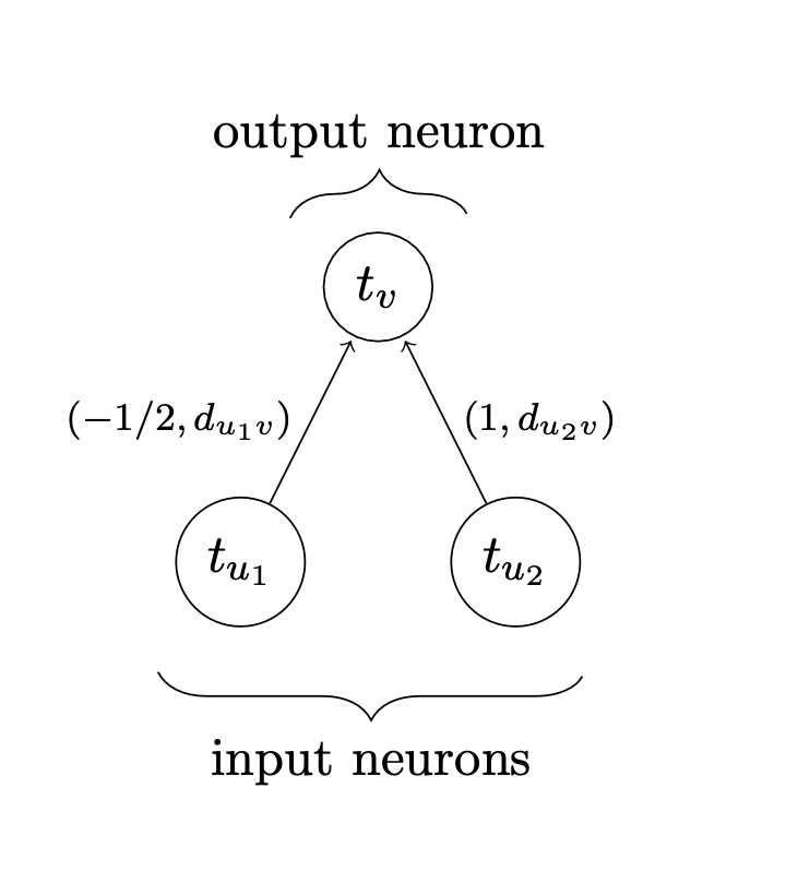
(a)

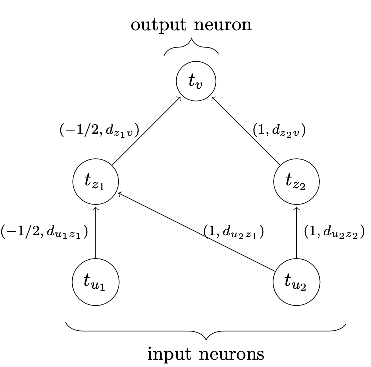
(b)

Figure 4: (a) Computation graph associated with a spiking network with two input neurons and one output neuron that realizes $f$ as defined in Proposition 3. (b) Stacking the network in (a) twice results in a spiking network that realizes the ReLU activation function.

Proposition 4.

Let $a<0<b<0.5\cdot c$ and consider $f:[a,b]\to\mathbb{R}$ defined as

$$f(x)=\begin{cases}x+c&,\text{ if }x>0\\ c&,\text{ if }x\leq 0\end{cases}$$

There exists a 2-layer SNN $\Phi$ with output neuron $v$ and input neuron $u_{1}$ such that $t_{v}(x)=f(x)$ on $[a,b]$, where $t_{v}(x)$ denotes the firing time of $v$ on input $t_{u_{1}}=x$.

Proof.

We introduce an auxiliary input neuron $u_{2}$ with constant firing time $t_{u_{2}}\in\mathbb{R}$ and specify the parameter of $\Phi=((W^{1},D^{1},\Theta^{1}),(W^{2},D^{2},\Theta^{2}))$ in the following manner:

$$W^{1}=\begin{pmatrix}-\frac{1}{2}&0\\ 1&2\end{pmatrix},D^{1}=\begin{pmatrix}d&0\\ d&\frac{d}{2}\end{pmatrix},\Theta^{1}=\begin{pmatrix}\theta\\ 2\theta\end{pmatrix},W^{2}=\begin{pmatrix}-\frac{1}{2}\\ 1\end{pmatrix},D^{2}=\begin{pmatrix}d\\ d\end{pmatrix},\Theta^{2}=\theta,$$ (21)

where $d\geq 0$ and $\theta>0$ is chosen such that $\theta+t_{u_{2}}>b$. We denote the input neurons by $u_{1},u_{2}$, the neurons in the hidden layer by $z_{1},z_{2}$ and the output neuron by $v$. Note that the firing time of $z_{1}$ depends on $u_{1}$ and $u_{2}$. In particular, either $u_{2}$ or $u_{1}$ together with $u_{2}$ can trigger a spike in $z_{1}$ since $w_{u_{1}z_{1}}<0$. Therefore, applying (7) yields that $u_{2}$ triggers a spike in $z_{1}$ under the following circumstances:

$$t_{z_{1}}(x)=\theta+t_{u_{2}}+d\quad\text{ if }t_{z_{1}}(x)\leq t_{u_{1}}+d=x+d.$$

Hence, this case only arises when

$$\theta+t_{u_{2}}+d\leq x+d\Leftrightarrow\theta+t_{u_{2}}\leq x.$$ (22)

However, by construction $\theta+t_{u_{2}}>b$, so that (22) does not hold for any $x\in[a,b]$. Thus, we conclude via (7) that

$$t_{z_{1}}(x)=2(\theta+t_{u_{2}}+d)-(x+d)=2(\theta+t_{u_{2}})+d-x.$$

By construction, the firing time $t_{z_{2}}=\theta+2t_{u_{2}}+d$ of $z_{2}$ is a constant which depends on the input only via $u_{2}$. A similar analysis as in the first layer shows that

$$t_{v}(x)=\theta+t_{z_{2}}+d\quad\text{ if }t_{v}(x)\leq t_{z_{1}}+d=2(\theta+t_{u_{2}})+d-x+d=2(\theta+t_{u_{2}}+d)-x.$$

Hence, $z_{2}$ triggers a spike in $v$ when

$$\theta+\theta+2t_{u_{2}}+d+d\leq 2(\theta+t_{u_{2}}+d)-x\quad\Leftrightarrow\quad x\leq 0.$$

If the additional condition

$$\theta+t_{z_{2}}+d=c\quad\Leftrightarrow\quad 2(\theta+d+t_{u_{2}})=c$$ (23)

is met, we can infer that

$$t_{v}(x) =\begin{cases}2(\theta+t_{z_{2}}+d)-(t_{z_{1}}(x)+d)&,\text{ if }x>0\\ \theta+t_{z_{2}}+d&,\text{ if }x\leq 0\end{cases}$$

$$=\begin{cases}2c-(2(\theta+t_{u_{2}})+d-x+d)&,\text{ if }x>0\\ c&,\text{ if }x\leq 0\end{cases}$$

$$=\begin{cases}x+c&,\text{ if }x>0\\ c&,\text{ if }x\leq 0\end{cases}.$$

Choosing $\theta$, $t_{u_{2}}$ and $d$ sufficiently small under the given constraints guarantees that $\eqref{eq:propCond22}$ holds, i.e., $\Phi$ emulates $f$ as desired. ∎

Remark 21.

It is again important to specify the encoding scheme via reference times $T_{\text{in}},T_{\text{out}}\in\mathbb{R}$, $T_{\text{in}}<T_{\text{out}}$ to ensure that $\Phi$ realizes ReLU. The input encoding $T_{\text{in}}-x$ and output decoding $T_{\text{out}}-t_{v}$ does not yield the desired output since it results in a realization of the type $-\text{ReLU}(-x)$. In contrast, the input encoding $T_{\text{in}}+x$ and output decoding $-T_{\text{out}}+t_{v}$ with $T_{\text{in}}=0$ and $T_{\text{out}}=c$ gives

$$\mathcal{R}_{\Phi}(x)=-T_{\text{out}}+t_{v}(T_{\text{in}}+x)=-T_{\text{out}}+f(T_{\text{in}}+x)=\begin{cases}x&,\text{ if }x>0\\ 0&,\text{ if }x\leq 0\end{cases}\,\,\,=\text{ReLU}(x).$$

In this case, it is necessary to choose the reference time $T_{\text{in}}=0$ to ensure that the breakpoint is also at zero. Next, we show that there is actually more freedom in choosing the reference time by analysing the construction in the proof more carefully.

Proposition 5.

Let $a<0<b$ and consider $f:[a,b]\to\mathbb{R}$ defined as

$$f(x)=\begin{cases}x&,\text{ if }x>0\\ 0&,\text{ if }x\leq 0\end{cases}$$

There exists a 2-layer SNN $\Phi$ with realization $\mathcal{R}_{\Phi}=f$ on $[a,b]$ with encoding scheme $T_{\text{in}}+x$ and decoding $-T_{\text{out}}+t_{v}$, where $v$ is the output neuron of $\Phi$, $T_{\text{in}}\in\mathbb{R}$ and $T_{\text{out}}=T_{\text{in}}+c$ for some constant $c>0$ depending on the parameters of $\Phi$.

Proof.

Performing a similar construction with the following changes and the same analysis as in the proof of Proposition 4 yields the claim. First, we slightly adjust $\Phi=((W^{1},D^{1},\Theta^{1}),(W^{2},D^{2},\Theta^{2}))$ in comparison to (21) and consider the network

$$W^{1}=\begin{pmatrix}-\frac{1}{2}&0\\ 1&1\end{pmatrix},D^{1}=\begin{pmatrix}d&0\\ d&d\end{pmatrix},\Theta^{1}=\begin{pmatrix}\theta\\ \theta\end{pmatrix},W^{2}=\begin{pmatrix}-\frac{1}{2}\\ 1\end{pmatrix},D^{2}=\begin{pmatrix}d\\ d\end{pmatrix},\Theta^{2}=\theta,$$

where $d\geq 0$ and $\theta>b$ are fixed (see Figure 4(b)). Second, we choose the input reference time $T_{\text{in}}\in\mathbb{R}$ and fix the input of the auxiliary input neuron $u_{2}$ as $t_{u_{2}}=T_{\text{in}}\in\mathbb{R}$. Finally, setting the output reference time $T_{\text{out}}=2(\theta+d)+T_{\text{in}}$ is sufficient to guarantee that $\Phi$ realizes $f$ on $[a,b]$. ∎

A.4 Realizing ReLU networks by spiking neural networks

In this section, we show that an SNN has the capability to reproduce the output of any ReLU network. Specifically, given access to the weights and biases of an ANN, we construct an SNN and set the parameter values based on the weights and biases of the given ANN. This leads us to the desired result. The essential part of our proof revolves around choosing the parameters of an SNN such that it effectively realizes the composition of an affine-linear map and the non-linearity represented by the ReLU activation. The realization of ReLU with SNNs is proved in the previous Section A.3. To realize an affine-linear function using a spiking neuron, it is necessary to ensure that the spikes from all the input neurons together result in the firing of an output neuron instead of any subset of the input neurons. We achieve that by appropriately adjusting the value of the threshold parameter. As a result, a spiking neuron, which implements an affine-linear map, avoids partitioning of the input space.

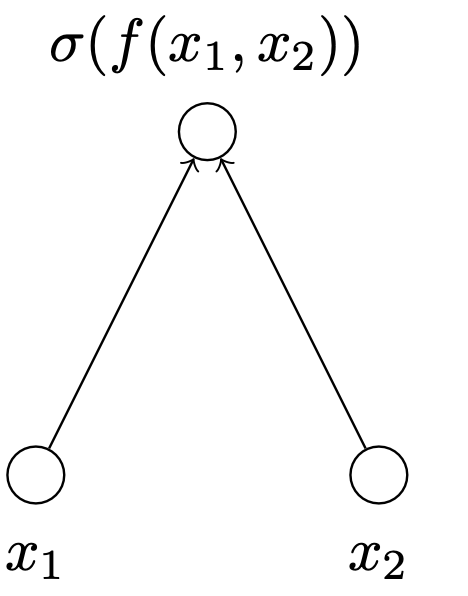
(a)

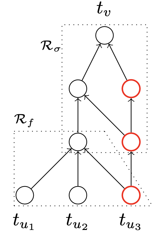
(b)

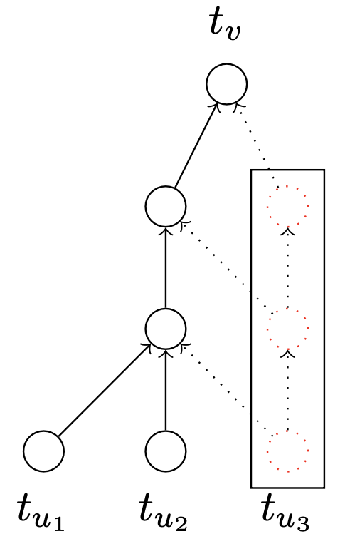
(c)

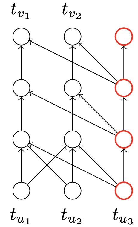
(d)

Figure 5: (a) Computation graph of an ANN with two input and one output unit realizing $\sigma(f(x_{1},x_{2}))$, where $\sigma$ is the ReLU activation function. (b) Computation graph associated with an SNN resulting from the concatenation of $\Phi^{\sigma}$ and $\Phi^{f}$ that realizes $\sigma(f(x_{1},x_{2}))$. The auxiliary neurons are shown in red. (c) Same computation graph as in (b); when parallelizing two identical networks, the dotted auxiliary neurons can be removed and auxiliary neurons from (b) can be used for each network instead. (d) Computation graph associated with a spiking network as a result of the parallelization of two subnetworks $\Phi^{\sigma\circ f_{1}}$ and $\Phi^{\sigma\circ f_{2}}$. The auxiliary neuron in the output layer serves the same purpose as the auxiliary neuron in the input layer and is needed when concatenating two such subnetworks $\Phi_{\sigma\circ f}$.

Setup for the proof of Theorem 3

Let $d,L\in\mathbb{N}$ be the width and the depth of an ANN $\Psi$, respectively, i.e.,

$$\Psi=((A^{1},B^{1}),(A^{2},B^{2}),\dots,(A^{L},B^{L})),\text{ where } (A^{\ell},B^{\ell})\in\mathbb{R}^{d\times d}\times\mathbb{R}^{d},1\leq\ell<L,$$

$$(A^{L},B^{L})\in\mathbb{R}^{1\times d}\times\mathbb{R}.$$

For a given input domain $[a,b]^{d}\subset\mathbb{R}^{d}$, we denote by $\Psi^{\ell}=((A^{\ell},B^{\ell}))$ the $\ell$-th layer, where $y^{0}\in[a,b]^{d}$ and

$$y^{l} =\mathcal{R}_{\Psi^{l}}(y^{l-1})=\sigma(A^{l}y^{l-1}+B^{l}),1\leq\ell<L,$$

$$y^{L} =\mathcal{R}_{\Psi^{L}}(y^{L-1})=A^{L}y^{L-1}+B^{L}$$ (24)

so that $\mathcal{R}_{\Psi}=\mathcal{R}_{\Psi^{L}}\circ\cdots\circ\mathcal{R}_{\Psi^{1}}$.

For the construction of the corresponding SNN we refer to the associated weights and delays between two spiking neurons $u$ and $v$ by $w_{uv}$ and $d_{uv}$, respectively.

Proof of Theorem 3.

Any multi-layer ANN $\Psi$ with ReLU activation is simply an alternating composition of affine-linear functions $A^{l}y^{l-1}+B^{l}$ and a non-linear function represented by $\sigma$. To generate the mapping realized by $\Psi$, it suffices to realize the composition of affine-linear functions and the ReLU non-linearity and then extend the construction to the whole network using concatenation and parallelization operations. We prove the result via the following steps; see also Figure 5 for a depiction of the intermediate constructions.

Step 1: Realizing ReLU non-linearity.
Proposition 5 gives the desired result.

Step 2: Realizing affine-linear functions with one-dimensional range.
Let $f:[a,b]^{d}\to\mathbb{R}$ be an affine-linear function

$$f(x)=C^{T}x+s,\quad C^{T}=(c_{1},\dots,c_{d})\in\mathbb{R}^{d},s\in\mathbb{R}.$$ (25)

Consider a one-layer SNN that consists of an output neuron $v$ and d input units $u_{1},\dots,u_{d}$. Via (7) the firing time of $v$ as a function of the input firing times on the linear region $R^{I}$ corresponding to the index set $I=\{1,\dots,d\}$ is given by

$$t_{v}(t_{u_{1}},\dots,t_{u_{d}})=\frac{\theta_{v}}{\sum_{i\in I}w_{u_{i}v}}+\frac{\sum_{i\in I}w_{u_{i}v}(t_{u_{i}}+d_{u_{i}v})}{\sum_{i\in I}w_{u_{i}v}}\quad\text{provided that }\sum_{i\in I}w_{u_{i}v}>0.$$

Introducing an auxiliary input neuron $u_{d+1}$ with weight $w_{u_{d+1}v}=1-\sum_{i\in I}w_{u_{i}v}$ ensures that $\sum_{i\in I\cup\{d+1\}}w_{u_{i}v}>0$ and leads to the firing time

$$t_{v}(t_{u_{1}},\dots,t_{u_{d+1}})=\theta_{v}+\sum_{i\in I\cup\{d+1\}}w_{u_{i}v}(t_{u_{i}}+d_{u_{i}v})\quad\text{ on }R^{I\cup\{d+1\}}.$$

Setting $w_{u_{i}v}=c_{i}$ for $i\in I$ and $d_{u_{j}v}=d^{\prime}\geq 0$ for $j\in I\cup\{d+1\}$ yields

$$t_{v}(t_{u_{1}},\dots,t_{u_{d+1}})=\theta_{v}+w_{u_{d+1}v}\cdot t_{u_{d+1}}+d^{\prime}+\sum_{i\in I}c_{i}t_{u_{i}}\text{ on }R^{I\cup\{d+1\}}\cap[a,b]^{d}.$$

Therefore, an SNN $\Phi^{f}=(W,D,\Theta)$ with parameters

$$W=\begin{pmatrix}c_{1}\\ \vdots\\ c_{d+1}\end{pmatrix},D=\begin{pmatrix}d^{\prime}\\ \vdots\\ d^{\prime}\end{pmatrix},\Theta=\theta>0,\quad\text{ where }c_{d+1}=1-\sum_{i\in I}c_{i},$$

and the usual encoding scheme $T_{\text{in}}/T_{\text{out}}+\cdot$ and fixed firing time $t_{u_{d+1}}=T_{\text{in}}\in\mathbb{R}$ realizes

$$\mathcal{R}_{\Phi^{f}}(x) =-T_{\text{out}}+t_{v}(T_{\text{in}}+x_{1},\dots,T_{\text{in}}+x_{d},T_{\text{in}})=-T_{\text{out}}+\theta+T_{\text{in}}+d^{\prime}+\sum_{i\in I}c_{i}x_{i}$$ (26)

$$=-T_{\text{out}}+\theta+T_{\text{in}}+d^{\prime}+f(x_{1},\dots,x_{d})-s\quad\text{ on }R^{I\cup\{d+1\}}\cap[a,b]^{d}.$$ (27)

Choosing a large enough threshold $\theta$ ensures that a spike in $v$ is necessarily triggered after all the spikes from $u_{1},\dots,u_{d+1}$ reached $v$ so that $[a,b]^{d}\subset R^{I\cup\{d+1\}}$ holds. It suffices to set

$$\theta\geq\sup_{x\in[a,b]^{d}}\sup_{x_{\text{min}}\leq t-T_{\text{in}}-d^{\prime}\leq x_{\text{max}}}P_{v}(t),$$

where $x_{\text{min}}=\min\{x_{1},\dots,x_{d},0\}$ and $x_{\text{max}}=\max\{x_{1},\dots,x_{d},0\}$, since this implies that the potential $P_{v}(t)$ is smaller than the threshold to trigger a spike in $v$ on the time interval associated to feasible input spikes, i.e., $v$ emits a spike after the last spike from an input neuron arrived at $v$. Applying (5) shows that for $x\in[a,b]^{d}$ and $t\in[x_{\text{min}}+T_{\text{in}}+d^{\prime},x_{\text{max}}+T_{\text{in}}+d^{\prime}]$

$$P_{v}(t) =\sum_{i\in I}w_{u_{i}v}(t-(T_{\text{in}}+x_{i})-d_{u_{i}v})+w_{u_{d+1}v}(t-T_{\text{in}}-d_{u_{d+1}v})=t-d^{\prime}-T_{\text{in}}+\sum_{i\in I}c_{i}x_{i}$$

$$\leq x_{\text{max}}+d\left\lVert C\right\rVert_{\infty}\left\lVert x\right\rVert_{\infty}\leq(1+d\left\lVert C\right\rVert_{\infty})\max\{|a|,|b|\}.$$

Hence, we set

$$\theta=(1+d\left\lVert C\right\rVert_{\infty})\max\{|a|,|b|\}+s+|s|\quad\text{ and }\quad T_{\text{out}}=\theta-s+T_{\text{in}}+d^{\prime}$$

to obtain via (26) that

$$\mathcal{R}_{\Phi^{f}}(x)=-T_{\text{out}}+t_{v}(T_{\text{in}}+x_{1},\dots,T_{\text{in}}+x_{d},T_{\text{in}})=f(x)\quad\text{ for }x\in[a,b]^{d}.$$ (28)

Note that the reference time $T_{\text{out}}=(1+d\left\lVert C\right\rVert_{\infty})\max\{|a|,|b|\}+|s|+T_{\text{in}}+d^{\prime}$ is independent of the specific parameters of $f$ in the sense that only upper bounds $\left\lVert C\right\rVert_{\infty},|s|$ on the parameters are relevant. Therefore, $T_{\text{out}}$ (with the associated choice of $\theta$) can be applied for different affine linear functions as long as the upper bounds remain valid. This is necessary for the composition and parallelization of subnetworks in the subsequent construction.

Step 3: Realizing compositions of affine-linear functions with one-dimensional range and ReLU.
The next step is to realize the composition of ReLU $\sigma$ with an affine linear mapping $f$ defined in (25). To that end, we want to concatenate the networks $\Phi^{\sigma}$ and $\Phi^{f}$ constructed in Step 1 and Step 2, respectively, via Lemma 1. To employ the concatenation operation we need to perform the following steps:

1. Find an appropriate input domain $[a^{\prime},b^{\prime}]\subset\mathbb{R}$, that contains the image $f([a,b]^{d})$ so that parameters and reference times of $\Phi^{\sigma}$ can be fixed appropriately (see Proposition 5 for the detailed conditions on how to choose the parameter).

2. Ensure that the output reference time $T^{f}_{\text{out}}$ of $\Phi^{f}$ equals the input reference time $T^{\sigma}_{\text{in}}$ of $\Phi^{\sigma}$.

3. Ensure that the number of neurons in the output layer of $\Phi^{f}$ is the same as the number of input neurons in $\Phi^{\sigma}$.

For the first point, note that

$$|f(x)|=|C^{T}x+s|\leq d\left\lVert C\right\rVert_{\infty}\cdot\left\lVert x\right\rVert_{\infty}+|s|\leq d\left\lVert C\right\rVert_{\infty}\cdot\max\{|a|,|b|\}+|s|\text{ for all }x\in[a,b]^{d}.$$

Hence, we can use the input domain

$$[a^{\prime},b^{\prime}]=[-d\left\lVert C\right\rVert_{\infty}\cdot\max\{|a|,|b|\}+|s|,d\left\lVert C\right\rVert_{\infty}\cdot\max\{|a|,|b|\}+|s|]$$

and specify the parameters of $\Phi^{\sigma}$ accordingly. Additionally, recall from Proposition 5 that $T^{\sigma}_{\text{in}}$ can be chosen freely, so we may fix $T^{\sigma}_{\text{in}}=T^{f}_{\text{out}}$, where $T^{f}_{\text{out}}$ is established in Step 2. It remains to consider the third point. In order to realize ReLU an additional auxiliary neuron in the input layer of $\Phi^{\sigma}$ with constant input $T^{\sigma}_{\text{in}}$ was introduced. Hence, we also need to add an additional output neuron in $\Phi^{f}$ with (constant) firing time $T^{f}_{\text{out}}=T^{\sigma}_{\text{in}}$ so that the corresponding output and input dimension and their specification match. This is achieved by introducing a single synapse from the auxiliary neuron in the input layer of $\Phi^{f}$ to the newly added output neuron and by specifying the parameters of the newly introduced synapse and neuron suitably. Formally, the adapted network $\Phi^{f}=(W,D,\Theta)$ is given by

$$W=\begin{pmatrix}c_{1}&0\\ \vdots&\vdots\\ c_{d}&0\\ c_{d+1}&1\end{pmatrix},D=\begin{pmatrix}d^{\prime}&0\\ \vdots&\vdots\\ d^{\prime}&0\\ d^{\prime}&d^{\prime}\end{pmatrix},\Theta=\begin{pmatrix}\theta\\ T^{f}_{\text{out}}-T^{f}_{\text{in}}-d^{\prime}\end{pmatrix},$$

where the values of the parameters are specified in Step 2.

Then the realization of the concatenated network $\Phi^{\sigma\circ f}$ is the composition of the individual realizations. This is exemplarily demonstrated in Figure 5(b) for the two-dimensional input case. By analyzing $\Phi^{\sigma\circ f}$, we conclude that a three-layer SNN with

$$N(\Phi^{\sigma\circ f})=N(\Phi^{\sigma})-N_{0}(\Phi^{\sigma})+N(\Phi^{f})=5-2+d+3=d+6$$

computational units can realize $\sigma\circ f$ on $[a,b]^{d}$, where $N_{0}(\Phi^{\sigma})$ denotes the number of neurons in the input layer of $\Phi^{\sigma}$.

Step 4: Realizing layer-wise computation of $\Psi$.
The computations performed in a layer $\Psi^{\ell}$ of $\Psi$ are described in (4). Hence, for $1\leq\ell<L$ the computation can be expressed as

$$\mathcal{R}_{\Psi^{\ell}}(y^{l-1})=\sigma(A^{l}y^{l-1}+B^{l})=\begin{pmatrix}\sigma(\sum_{i=1}^{d}A_{1,i}^{l}y_{i}^{l-1}+B_{1}^{l})\\ \vdots\\ \sigma(\sum_{i=1}^{d}A_{d,i}^{l}y_{i}^{l-1}+B_{d}^{l})\end{pmatrix}=:\begin{pmatrix}\sigma(f_{1}(y^{l-1}))\\ \vdots\\ \sigma(f_{d}(y^{l-1}))\end{pmatrix},$$

where $f^{\ell}_{1},\dots,f^{\ell}_{d}$ are affine linear functions with one-dimensional range on the same input domain $[a^{\ell-1},b^{\ell-1}]\subset\mathbb{R}^{d}$, where $[a^{0},b^{0}]=[a,b]$ and $[a^{\ell},b^{\ell}]$ is the range of

$$(\sigma\circ f^{\ell-1}_{1},\dots,\sigma\circ f^{\ell-1}_{d})([a^{\ell-1},b^{\ell-1}]^{d}).$$

Thus, via Step 3, we construct SNNs $\Phi^{\ell}_{1},\dots,\Phi^{\ell}_{d}$ that realize $\sigma\circ f^{\ell}_{1},\dots,\sigma\circ f^{\ell}_{d}$ on $[a^{\ell-1},b^{\ell-1}]$. Note that by choosing appropriate parameters in the construction performed in Step 2 (as described below (28)), e.g., $\left\lVert A^{l}\right\rVert_{\infty}$ and $\left\lVert B^{l}\right\rVert_{\infty}$, we can employ the same input and output reference time for each $\Phi^{\ell}_{1},\dots,\Phi^{\ell}_{d}$. Consequently, we can parallelize $\Phi^{\ell}_{1},\dots,\Phi^{\ell}_{d}$ (see Lemma 2) and obtain networks $\Phi^{\ell}=P(\Phi^{\ell}_{1},\dots,\Phi^{\ell}_{d})$ realizing $\mathcal{R}_{\Psi^{\ell}}$ on $[a^{\ell-1},b^{\ell-1}]$. Finally, $\Psi^{L}$ can be directly realized via Step 2 by an SNN $\Phi^{L}$ (as in the last layer no activation function is applied and the output is one-dimensional). Although $\Phi^{\ell}$ already performs the desired task of realizing $\mathcal{R}_{\Psi^{\ell}}$ we can slightly simplify the network. By construction in Step 3, each $\Phi^{\ell}_{i}$ contains two auxiliary neurons in the hidden layers. Since the input and output reference time is chosen consistently for $\Phi^{\ell}_{1},\dots,\Phi^{\ell}_{d}$, we observe that the auxiliary neurons in each $\Phi^{\ell}_{i}$ perform the same operations and have the same firing times. Therefore, without changing the realization of $\Phi^{\ell}$ we can remove the auxiliary neurons in $\Phi^{\ell}_{2},\dots,\Phi^{\ell}_{d}$ and introduce synapses from the auxiliary neurons in $\Phi^{\ell}_{1}$ accordingly. This is exemplarily demonstrated in Figure 5(c) for the case $d=2$. After this modification, we observe that $L(\Phi^{\ell})=L(\Phi^{\ell}_{i})=3$ and

$$N(\Phi^{\ell}) =N(\Phi^{\ell}_{1})+\sum_{i=2}^{d}\big{(}N(\Phi^{\ell}_{i})-2-N_{0}(\Phi^{\ell}_{i})\big{)}=dN(\Phi^{\ell}_{1})-(d-1)(2+N_{0}(\Phi^{\ell}_{1}))$$

$$=d(d+6)-2(d-1)-(d-1)(d+1)=4d+3\quad\text{ for }1\leq\ell<L,$$

whereas $L(\Phi^{L})=1$ and $N(\Phi^{L})=d+2$.

Step 5: Realizing compositions of layer-wise computations of $\Psi$.
The last step is to compose the realizations $\mathcal{R}_{\Phi^{1}},\dots,\mathcal{R}_{\Phi^{L}}$ to obtain the realization

$$\mathcal{R}_{\Phi^{L}}\circ\cdots\circ\mathcal{R}_{\Phi^{1}}=\mathcal{R}_{\Psi^{L}}\circ\cdots\circ\mathcal{R}_{\Psi^{1}}=\mathcal{R}_{\Psi}.$$

As in Step 3, it suffices again to verify that the concatenation of the networks $\mathcal{R}_{\Phi^{1}},\dots,\mathcal{R}_{\Phi^{L}}$ is feasible. First, note that for $\ell=1,\dots,L$ the input domain of $\mathcal{R}_{\Phi^{\ell}}$ is given by $[a^{\ell-1},b^{\ell-1}]$ so that, we can fix the suitable output reference time $T^{\Phi^{\ell}}_{\text{out}}$ based on the parameters of the network, the input domain $[a^{\ell-1},b^{\ell-1}]$, and some input reference time $T^{\Phi^{\ell}}_{\text{in}}\in\mathbb{R}$. By construction in Steps 2 - 4 $T^{\Phi^{\ell}}_{\text{in}}$ can be chosen freely. Hence setting $T^{\Phi^{\ell+1}}_{\text{in}}=T^{\Phi^{\ell}}_{\text{out}}$ ensures that the reference times of the corresponding networks agree. It is left to align the input dimension of $\Phi^{\ell+1}$ and the output dimension of $\Phi^{\ell}$ for $\ell=1,\dots,L-1$. Due to the auxiliary neuron in the input layer of $\Phi^{\ell+1}$, we also need to introduce an auxiliary neuron in the output layer of $\Phi^{\ell}$ (see Figure 5(d)) with the required firing time $T^{\Phi^{\ell+1}}_{\text{in}}=T^{\Phi^{\ell}}_{\text{out}}$. Similarly, as in Step 3, it suffices to add a single synapse from the auxiliary neuron in the previous layer to obtain the desired firing time.

Thus, we conclude that $\Phi=\Phi^{L}\bullet\cdots\bullet\Phi^{1}$ realizes $\mathcal{R}_{\Psi}$ on $[a,b]$, as desired. The complexity of $\Phi$ in the number of layers and neurons is given by

$$L(\Phi)=\sum_{\ell=1}^{L}L(\Phi^{\ell})=3L-2=3L(\Psi)-2$$

and

$$N(\Phi) =N(\Phi^{1})+\sum_{\ell=2}^{L}\big{(}N(\Phi^{\ell})-N_{0}(\Phi^{\ell})\big{)}+(L-1)$$

$$=4d+3+(L-2)(4d+3-(d+1))+(d+2-(d+1))+(L-1)$$

$$=3L(d+1)-(2d+1)$$

$$=N(\Psi)+L(2d+3)-(2d+2)$$

∎

Remark 22.

Note that the delays play no significant role in the proof of the above theorem. Nevertheless, they can be employed to alter the timing of spikes, consequently impacting the firing time and the resulting output. However, the exact function of delays requires further investigation. The primary objective is to present a construction that proves the existence of a spiking network capable of accurately reproducing the output of any ReLU network.

A.5 Proof of Example 1

Recall the function introduced in Example 1,

$$f(x)=\begin{cases}x,&x\leq-\theta\\ \frac{x-\theta}{2},&-\theta<x<\theta\\ 0,&\,x\geq\theta\end{cases}\quad=-\frac{1}{2}\sigma(-x-\theta)-\frac{1}{2}\sigma(-x+\theta)\quad\text{for}\>\>x\in[a,b]\subset\mathbb{R},\theta>0,$$

that provides insights under which circumstances SNNs may express some target function with lower complexity than any corresponding ReLU-ANN.

Proof of Example 1.

First, we realize $f$ using spiking neurons. Consider an SNN $\Phi=(W,D,\Theta)$,

$$W=\begin{pmatrix}1\\ 1\end{pmatrix},D=\begin{pmatrix}d\\ d\end{pmatrix},\Theta=\theta$$

where $d\geq 0$. Denote the input neurons by $u_{1}$ and $u_{2}$ and the output neuron by $v$. We set the input and output reference times to $T_{\text{in}}=a$ and $T_{\text{out}}=\theta+T_{\text{in}}+d$, respectively. Following the usual encoding scheme, the input neuron $u_{1}$ fires at time $t_{u_{1}}=T_{\text{in}}+x$ and we fix $t_{u_{2}}=T_{\text{in}}$. Next, we consider two cases $(1)\left\lvert x\right\rvert\geq\theta$ and $(2)\left\lvert x\right\rvert<\theta$.

Case (1) In this case, an isolated spike from either one of the two input neurons causes the output neuron $v$ to fire at time $t_{v}$. In particular, if $x$ is negative, then $u_{1}$ triggers the spike in $v$, whereas, if $x$ is positive, then $u_{2}$ triggers the spike in $v$. Using equation (7), it can be directly verified that $t_{v}=T_{\text{out}}+f(x)$, i.e, $\mathcal{R}_{\Phi}(x)=f(x)$ for $\left\lvert x\right\rvert\geq\theta$.

Case (2) In this case, a spike in $v$ will be triggered by both the input neurons. By using equation (7), we observe that $t_{v}=T_{\text{out}}+\frac{x-\theta}{2}$, i.e, $\mathcal{R}_{\Phi}(x)=f(x)$ for $\left\lvert x\right\rvert<\theta$.

Next, observe that $f$ can be realized using a two-layer ReLU-ANN $\Psi=((A^{1},B^{1}),(A^{2},B^{2}))$ with two units in the hidden layer and one output unit, where

$$A^{1}=\begin{pmatrix}-1&-1\end{pmatrix},\quad B^{1}=\begin{pmatrix}-\theta&\theta\end{pmatrix},\quad A^{2}=\begin{pmatrix}-0.5\\ -0.5\end{pmatrix},\quad B^{2}=0.$$

Moreover, note that $\Psi$ is optimal in terms of complexity. Indeed, a single ReLU unit with any number of incoming edges separates the input space into at most two linear regions. Since $f$ has three different linear regions, it is not possible to capture all the linear regions by a single ReLU unit. Hence, at least two hidden units, i.e., four units with input and output, and two layers are needed realize $f$ via a ReLU-ANN. ∎

References

- Abe [91] M. Abeles. Corticonics: Neural Circuits of the Cerebral Cortex. Cambridge University Press, 1991.
- ABMM [18] Raman Arora, Amitabh Basu, Poorya Mianjy, and Anirbit Mukherjee. Understanding deep neural networks with rectified linear units. In International Conference on Learning Representations, ICLR, 2018.
- BGKP [22] Julius Berner, Philipp Grohs, Gitta Kutyniok, and Philipp Petersen. The modern mathematics of deep learning. In Mathematical Aspects of Deep Learning, pages 1–111. Cambridge University Press, dec 2022.
- BHLM [19] Peter L. Bartlett, Nick Harvey, Christopher Liaw, and Abbas Mehrabian. Nearly-tight VC-dimension and pseudodimension bounds for piecewise linear neural networks. Journal of Machine Learning Research, 20(63):1–17, 2019.
- BKP [01] Sander Bohte, Joost Kok, and Han Poutré. Error-backpropagation in temporally encoded networks of spiking neurons. Neurocomputing, 48:17–37, 02 2001.
- BMM [99] Peter Bartlett, Vitaly Maiorov, and Ron Meir. Almost linear VC dimension bounds for piecewise polynomial networks. Neural Computation, 10, 1999.
- BMR+ [20] Tom Brown, Benjamin Mann, Nick Ryder, Melanie Subbiah, Jared D Kaplan, Prafulla Dhariwal, Arvind Neelakantan, Pranav Shyam, Girish Sastry, Amanda Askell, Sandhini Agarwal, Ariel Herbert-Voss, Gretchen Krueger, Tom Henighan, Rewon Child, Aditya Ramesh, Daniel Ziegler, Jeffrey Wu, Clemens Winter, Chris Hesse, Mark Chen, Eric Sigler, Mateusz Litwin, Scott Gray, Benjamin Chess, Jack Clark, Christopher Berner, Sam McCandlish, Alec Radford, Ilya Sutskever, and Dario Amodei. Language models are few-shot learners. In H. Larochelle, M. Ranzato, R. Hadsell, M.F. Balcan, and H. Lin, editors, Advances in Neural Information Processing Systems, volume 33, pages 1877–1901. Curran Associates, Inc., 2020.
- CDLB+ [22] Dennis Valbjørn Christensen, Regina Dittmann, Bernabe Linares-Barranco, Abu Sebastian, Manuel Le Gallo, Andrea Redaelli, Stefan Slesazeck, Thomas Mikolajick, Sabina Spiga, Stephan Menzel, Ilia Valov, Gianluca Milano, Carlo Ricciardi, Shi-Jun Liang, Feng Miao, Mario Lanza, Tyler J. Quill, Scott Tom Keene, Alberto Salleo, Julie Grollier, Danijela Markovic, Alice Mizrahi, Peng Yao, J. Joshua Yang, Giacomo Indiveri, John Paul Strachan, Suman Datta, Elisa Vianello, Alexandre Valentian, Johannes Feldmann, Xuan Li, Wolfram HP Pernice, Harish Bhaskaran, Steve Furber, Emre Neftci, Franz Scherr, Wolfgang Maass, Srikanth Ramaswamy, Jonathan Tapson, Priyadarshini Panda, Youngeun Kim, Gouhei Tanaka, Simon Thorpe, Chiara Bartolozzi, Thomas A Cleland, Christoph Posch, Shih-Chii Liu, Gabriella Panuccio, Mufti Mahmud, Arnab Neelim Mazumder, Morteza Hosseini, Tinoosh Mohsenin, Elisa Donati, Silvia Tolu, Roberto Galeazzi, Martin Ejsing Christensen, Sune Holm, Daniele Ielmini, and Nini Pryds. 2022 Roadmap on Neuromorphic Computing and Engineering. Neuromorph. Comput. Eng., 2(2), 2022.
- [9] Iulia M. Comsa, Krzysztof Potempa, Luca Versari, Thomas Fischbacher, Andrea Gesmundo, and Jyrki Alakuijala. Temporal coding in spiking neural networks with alpha synaptic function. In ICASSP 2020 - 2020 IEEE International Conference on Acoustics, Speech and Signal Processing (ICASSP), pages 8529–8533, 2020.
- [10] Iulia M. Comsa, Krzysztof Potempa, Luca Versari, Thomas Fischbacher, Andrea Gesmundo, and Jyrki Alakuijala. Temporal coding in spiking neural networks with alpha synaptic function. In ICASSP 2020 - 2020 IEEE International Conference on Acoustics, Speech and Signal Processing (ICASSP), pages 8529–8533, 2020.
- Cyb [89] George V. Cybenko. Approximation by superpositions of a sigmoidal function. Mathematics of Control, Signals and Systems, 2:303–314, 1989.
- DDF+ [22] I. Daubechies, R. DeVore, S. Foucart, B. Hanin, and G. Petrova. Nonlinear Approximation and (Deep) ReLU Networks. Constructive Approximation, 55(1):127–172, 2022.
- DHP [21] Ronald DeVore, Boris Hanin, and Guergana Petrova. Neural network approximation. Acta Numerica, 30:327–444, 2021.
- DSD [20] Nadav Dym, Barak Sober, and Ingrid Daubechies. Expression of fractals through neural network functions. IEEE Journal on Selected Areas in Information Theory, 1(1):57–66, 2020.
- GBDHL+ [16] Rafael Gómez-Bombarelli, David Duvenaud, José Hernández-Lobato, Jorge Aguilera-Iparraguirre, Timothy Hirzel, Ryan Adams, and Alán Aspuru-Guzik. Automatic chemical design using a data-driven continuous representation of molecules. ACS Central Science, 4, 10 2016.
- Ger [95] Wulfram Gerstner. Time structure of the activity in neural network models. Phys. Rev. E, 51:738–758, 1995.
- GEU [22] Alexis Goujon, Arian Etemadi, and Michael A. Unser. The role of depth, width, and activation complexity in the number of linear regions of neural networks. ArXiv, abs/2206.08615, 2022.
- GJ [95] Paul W. Goldberg and Mark R. Jerrum. Bounding the Vapnik-Chervonenkis dimension of concept classes parameterized by real numbers. Machine Learning, 18(2):131–148, 1995.
- GK [02] Wulfram Gerstner and Werner M. Kistler. Spiking Neuron Models: Single Neurons, Populations, Plasticity. Cambridge University Press, Cambridge UK, 2002.
- GKB+ [21] J. Göltz, L. Kriener, Andreas Baumbach, S. Billaudelle, O. Breitwieser, B. Cramer, Dominik Dold, Akos Kungl, Walter Senn, Johannes Schemmel, Karlheinz Meier, and M. Petrovici. Fast and energy-efficient neuromorphic deep learning with first-spike times. Nature Machine Intelligence, 3:823–835, 09 2021.
- GKNP [14] Wulfram Gerstner, Werner M. Kistler, Richard Naud, and Liam Paninski. Neuronal Dynamics: From Single Neurons to Networks and Models of Cognition. Cambridge University Press, 2014.
- GRK [20] Ingo Gühring, Mones Raslan, and Gitta Kutyniok. Expressivity of deep neural networks. arXiv:2007.04759, 2020.
- GvH [93] Wulfram Gerstner and J. van Hemmen. How to describe neuronal activity: Spikes, rates, or assemblies? In Advances in Neural Information Processing Systems, volume 6. Morgan-Kaufmann, 1993.
- Hop [95] John Hopfield. Pattern recognition computation using action potential timing for stimulus representation. Nature, 376:33–6, 08 1995.
- KGH [97] Werner M. Kistler, Wulfram Gerstner, and J. Leo van Hemmen. Reduction of the Hodgkin-Huxley Equations to a Single-Variable Threshold Model. Neural Computation, 9(5):1015–1045, 1997.
- KKH+ [18] Jaehyun Kim, Heesu Kim, Subin Huh, Jinho Lee, and Kiyoung Choi. Deep neural networks with weighted spikes. Neurocomputing, 311:373–386, 2018.
- KSH [12] Alex Krizhevsky, Ilya Sutskever, and Geoffrey E Hinton. Imagenet classification with deep convolutional neural networks. In Advances in Neural Information Processing Systems, volume 25. Curran Associates, Inc., 2012.
- KZGK [22] Adar Kahana, Qian Zhang, Leonard Gleyzer, and George Em Karniadakis. Spiking neural operators for scientific machine learning, 2022.
- LBH [15] Yann LeCun, Yoshua Bengio, and Geoffrey Hinton. Deep learning. Nature, 521(7553):436–444, 2015.
- LSP+ [20] Chankyu Lee, Syed Shakib Sarwar, Priyadarshini Panda, Gopalakrishnan Srinivasan, and Kaushik Roy. Enabling spike-based backpropagation for training deep neural network architectures. Frontiers in Neuroscience, 14, 2020.
- Maa [95] Wolfgang Maass. An efficient implementation of sigmoidal neural nets in temporal coding with noisy spiking neurons. Technical report, Technische Universität Graz, 1995.
- [32] Wolfgang Maass. Lower bounds for the computational power of networks of spiking neurons. Neural Computation, 8(1):1–40, 1996.
- [33] Wolfgang Maass. Networks of spiking neurons: The third generation of neural network models. Electron. Colloquium Comput. Complex., 3, 1996.
- [34] Wolfgang Maass. Noisy spiking neurons with temporal coding have more computational power than sigmoidal neurons. In Advances in Neural Information Processing Systems, volume 9. MIT Press, 1996.
- Maa [01] Wolfgang Maass. On the relevance of time in neural computation and learning. Theoretical Computer Science, 261(1):157–178, 2001.
- MJJ [17] Akshay Kumar Maan, Deepthi Anirudhan Jayadevi, and Alex Pappachen James. A survey of memristive threshold logic circuits. IEEE Transactions on Neural Networks and Learning Systems, 28(8):1734–1746, 2017.
- Mos [18] Hesham Mostafa. Supervised learning based on temporal coding in spiking neural networks. IEEE Transactions on Neural Networks and Learning Systems, 29(7):3227–3235, 2018.
- MPCB [14] Guido Montúfar, Razvan Pascanu, Kyunghyun Cho, and Yoshua Bengio. On the number of linear regions of deep neural networks. In Proceedings of the 27th International Conference on Neural Information Processing Systems - Volume 2, NIPS’14, page 2924–2932, Cambridge, MA, USA, 2014. MIT Press.
- MRC [18] Hesham Mostafa, Vishwajith Ramesh, and Gert Cauwenberghs. Deep supervised learning using local errors. Frontiers in Neuroscience, 12, 2018.
- PV [18] Philipp Petersen and Felix Voigtlaender. Optimal approximation of piecewise smooth functions using deep relu neural networks. Neural Networks, 108:296–330, 2018.
- RHW [86] David E. Rumelhart, Geoffrey E. Hinton, and Ronald J. Williams. Learning representations by back-propagating errors. Nature, 323(6088):533–536, 1986.
- [42] Bodo Rueckauer and Shih-Chii Liu. Conversion of analog to spiking neural networks using sparse temporal coding. In 2018 IEEE International Symposium on Circuits and Systems (ISCAS), pages 1–5, 2018.
- [43] Bodo Rueckauer and Shih-Chii Liu. Conversion of analog to spiking neural networks using sparse temporal coding. In 2018 IEEE International Symposium on Circuits and Systems (ISCAS), pages 1–5, 2018.
- RL [21] Bodo Rueckauer and Shih-Chii Liu. Temporal pattern coding in deep spiking neural networks. In 2021 International Joint Conference on Neural Networks (IJCNN), pages 1–8, 2021.
- RLH+ [17] Bodo Rueckauer, Iulia-Alexandra Lungu, Yuhuang Hu, Michael Pfeiffer, and Shih-Chii Liu. Conversion of continuous-valued deep networks to efficient event-driven networks for image classification. Frontiers in Neuroscience, 11, 12 2017.
- SEC+ [22] Ana Stanojevic, Evangelos Eleftheriou, Giovanni Cherubini, Stanisław Woźniak, Angeliki Pantazi, and Wulfram Gerstner. Approximating Relu networks by single-spike computation. In 2022 IEEE International Conference on Image Processing (ICIP), pages 1901–1905, 2022.
- SHM+ [16] David Silver, Aja Huang, Christopher Maddison, Arthur Guez, Laurent Sifre, George Driessche, Julian Schrittwieser, Ioannis Antonoglou, Veda Panneershelvam, Marc Lanctot, Sander Dieleman, Dominik Grewe, John Nham, Nal Kalchbrenner, Ilya Sutskever, Timothy Lillicrap, Madeleine Leach, Koray Kavukcuoglu, Thore Graepel, and Demis Hassabis. Mastering the game of go with deep neural networks and tree search. Nature, 529:484–489, 01 2016.
- SKP+ [22] Catherine D. Schuman, Shruti R. Kulkarni, Maryam Parsa, J. Parker Mitchell, Prasanna Date, and Bill Kay. Opportunities for neuromorphic computing algorithms and applications. Nature Computational Science, 2(1):10–19, 2022.
- SM [21] Christoph Stöckl and Wolfgang Maass. Optimized spiking neurons can classify images with high accuracy through temporal coding with two spikes. Nature Machine Intelligence, 3:230–238, 03 2021.
- Ste [67] R. B. Stein. The information capacity of nerve cells using a frequency code. Biophysical journal, 7(6):797–826, 1967.
- SVC [04] B. Schrauwen and J. Van Campenhout. Extending spikeprop. In 2004 IEEE International Joint Conference on Neural Networks (IEEE Cat. No.04CH37541), volume 1, pages 471–475, 2004.
- SWB+ [22] Ana Stanojevic, Stanisław Woźniak, Guillaume Bellec, Giovanni Cherubini, Angeliki Pantazi, and Wulfram Gerstner. An exact mapping from ReLU networks to spiking neural networks. arXiv:2212.12522, 2022.
- TFM [96] Simon Thorpe, Denis Fize, and Catherine Marlot. Speed of processing in the human visual system. Nature, 381(6582):520–522, 1996.
- TGLM [21] Neil C. Thompson, Kristjan Greenewald, Keeheon Lee, and Gabriel F. Manso. Deep learning’s diminishing returns: The cost of improvement is becoming unsustainable. IEEE Spectrum, 58(10):50–55, 2021.
- TLD [17] Ping Tak Peter Tang, Tsung-Han Lin, and Mike Davies. Sparse coding by spiking neural networks: Convergence theory and computational results, 2017.
- TLI+ [23] Hugo Touvron, Thibaut Lavril, Gautier Izacard, Xavier Martinet, Marie-Anne Lachaux, Timothée Lacroix, Baptiste Rozière, Naman Goyal, Eric Hambro, Faisal Azhar, Aurelien Rodriguez, Armand Joulin, Edouard Grave, and Guillaume Lample. Llama: Open and efficient foundation language models, 2023.
- VSP+ [17] Ashish Vaswani, Noam Shazeer, Niki Parmar, Jakob Uszkoreit, Llion Jones, Aidan N. Gomez, Łukasz Kaiser, and Illia Polosukhin. Attention is all you need. In Neural Information Processing Systems, 2017.
- WDL+ [18] Yujie Wu, Lei Deng, Guoqi Li, Jun Zhu, and Luping Shi. Spatio-temporal backpropagation for training high-performance spiking neural networks. Frontiers in Neuroscience, 12, 2018.
- Yar [17] Dmitry Yarotsky. Error bounds for approximations with deep relu networks. Neural Networks, 94:103–114, 2017.
- YHH+ [19] Amirreza Yousefzadeh, Sahar Hosseini, Priscila Holanda, Sam Leroux, Thilo Werner, Teresa Serrano-Gotarredona, Bernabe Linares Barranco, Bart Dhoedt, and Pieter Simoens. Conversion of synchronous artificial neural network to asynchronous spiking neural network using sigma-delta quantization. In 2019 IEEE International Conference on Artificial Intelligence Circuits and Systems (AICAS), pages 81–85, 2019.
- YZW [21] Zhanglu Yan, Jun Zhou, and Weng-Fai Wong. Near lossless transfer learning for spiking neural networks. Proceedings of the AAAI Conference on Artificial Intelligence, 35(12):10577–10584, May 2021.
- ZZ [22] Shao-Qun Zhang and Zhi-Hua Zhou. Theoretically provable spiking neural networks. In S. Koyejo, S. Mohamed, A. Agarwal, D. Belgrave, K. Cho, and A. Oh, editors, Advances in Neural Information Processing Systems, volume 35, pages 19345–19356. Curran Associates, Inc., 2022.
- ZZZ+ [19] Lei Zhang, Shengyuan Zhou, Tian Zhi, Zidong Du, and Yunji Chen. Tdsnn: From deep neural networks to deep spike neural networks with temporal-coding. Proceedings of the AAAI Conference on Artificial Intelligence, 33(01):1319–1326, Jul. 2019.