Efficient relaxation scheme for the SIR and related compartmental models

Abstract

In this paper, we introduce a novel numerical approach for approximating the SIR model in epidemiology. Our method enhances the existing linearization procedure by incorporating a suitable relaxation term to tackle the transcendental equation of nonlinear type. Developed within the continuous framework, our relaxation method is explicit and easy to implement, relying on a sequence of linear differential equations. This approach yields accurate approximations in both discrete and analytical forms. Through rigorous analysis, we prove that, with an appropriate choice of the relaxation parameter, our numerical scheme is non-negativity-preserving and globally strongly convergent towards the true solution. These theoretical findings have not received sufficient attention in various existing SIR solvers. We also extend the applicability of our relaxation method to handle some variations of the traditional SIR model. Finally, we present numerical examples using simulated data to demonstrate the effectiveness of our proposed method.

I Introduction

In recent years, the world has witnessed the devastating impact of infectious diseases on a global scale. From the rapid spread of COVID-19 to the resurgence of long-standing ailments like measles and influenza, understanding the dynamics of epidemics has become crucial for protecting public health. To gain a deeper understanding of these intricate phenomena, scientists have increasingly relied on mathematical modeling as an influential tool for unraveling the complex mechanisms governing disease transmission. Among the various models, the Susceptible-Infectious-Recovered (SIR) model has emerged as a fundamental framework, providing valuable insights into epidemic dynamics; cf. e.g. [7, 11, 15] for its applications to modeling the influenza, Ebola and COVID-19.

The SIR model, initially proposed in the early 20th century by Kermack and McKendrick [10], has since been refined and adapted to address contemporary challenges. This model effectively captures the fundamental dynamics of epidemics by dividing a population into three distinct compartments: susceptible individuals, infectious individuals, and removed individuals. By considering the interactions between these compartments, the SIR model takes into account various factors such as transmission rates, removal rates, and the depletion of susceptible individuals over time. The “removals” in this context encompass individuals who are isolated, deceased, or have recovered and gained immunity. Additionally, the model assumes that individuals who have gained immunity or recovered enter a new category that is not susceptible to the disease.

Consider a homogeneously mixed group of individuals of total size $N\gg 1$. Let $t\in\left(0,T\right)$ be the time variable with $T>0$ being the final time of observations. We take into account the following functions:

$$S\left(t\right) =\text{number of susceptibles at time }t,$$

$$I\left(t\right) =\text{number of infectives at time }t,$$

$$R\left(t\right) =\text{number of removals at time }t.$$

Initiated, again, by Kermack and McKendrick in 1927 [10], the evolutionary dynamics of these individuals can be modeled through the following system of ordinary differential equations (ODEs):

$$\begin{cases}I^{\prime}\left(t\right)=\beta S\left(t\right)I\left(t\right)-\gamma I\left(t\right),\\ S^{\prime}\left(t\right)=-\beta S\left(t\right)I\left(t\right),\\ R^{\prime}\left(t\right)=\gamma I\left(t\right).\end{cases}$$ (I.1)

Here, the following assumptions are considered.

(A1) The total population size is always $N>0$, meaning that $S\left(t\right)+I\left(t\right)+R\left(t\right)=N$ for all $t$.

(A2) We know the infection rate $\beta>0$ from the infection process, and the removal rate $\gamma>0$ from the removal process.

(A3) The initial conditions are $S\left(0\right)=n>1$, $I\left(0\right)=a\geq 1$ and $R\left(0\right)=0$.

The explicit solution of the SIR model, despite its basic structure, is widely known to be unattainable due to the exponential nonlinearity of the transcendental equation governing removals. Consequently, numerous numerical methods have been proposed to address this fundamental model. The Taylor expansion method, initially employed by Kermack and McKendrick in 1927, approximates the exponential term, leading to an approximate analytic solution. This technique was utilized to simulate the plague epidemic of 1905-1906 in Bombay, India, and has since become a tutorial resource for students at both undergraduate and graduate levels; cf. [4].

Over the years, many different methods have been studied to solve the SIR model. Piyawong et al. [20] introduced an unconditionally convergent scheme that captures the long-term behavior of the SIR model, offering improved numerical stability compared to conventional explicit finite difference methods. Mickens [18] and, recently, Conte et al. [6] proposed and analyzed stable nonstandard finite difference methods that effectively preserve the positivity of the SIR solutions. Semi-analytical methods, such as the Adomian decomposition approach [17], have also been proposed, alongside other methods cited therein, to derive approximate analytical solutions. Additionally, the solutions of the SIR model can be expressed in terms of the Lambert function, as demonstrated in the publications by [2, 21]. Furthermore, an alternative approach involving parametric analysis has been employed to obtain analytical solutions; see e.g. [9]. While most of these approaches are local approximations, a recent global semi-analytical approach utilizing the Padé approximation has been presented in [5].

While the above-mentioned approximation methods have demonstrated numerical effectiveness, their convergence theories have received limited investigation. Some publications discussing discrete methods focus solely on stability analysis, leaving the global convergence analysis unexplored. In this study, we propose a novel numerical approach that guarantees global convergence. Our approach employs a relaxation procedure, derived from the conventional linearization technique, to approximate the SIR model in a continuous setting. Unlike the classical version, our modified procedure introduces a relaxation term. In the existing literature on partial differential equations (e.g., [13, 14, 19, 25] and references cited therein), this relaxation term mitigates the local convergence issues encountered by conventional linearization techniques such as Newton’s method. Consequently, it permits to choose an arbitrary starting point while guaranteeing the global convergence. Within our specific context, the relaxation term facilitates capturing the non-negativity of solutions while preserving global convergence. In addition, by relying only on the dependence of the relaxation constant on the removal rate, our approach accurately captures the long-term behavior of the system. Besides, our explicit and easy-to-implement approximate scheme is governed by a sequence of linear differential equations. The desired approximate solution can be obtained discretely or analytically based on individual preference.

Our paper is four-fold. In section II, we begin by revisiting the transcendental equation for removals and discussing the essential properties of the SIR model. The latter part of this section focuses on introducing the proposed relaxation scheme and establishing its theoretical foundations. We prove that this scheme is globally strongly convergent and preserves non-negativity. Additionally, we derive an error estimate in $C^{0}$. In section III, we extend the applicability of our proposed scheme to some variants of the SIR model. Then, to validate the effectiveness of our method, numerical examples are presented in Section IV. Finally, we provide some concluding remarks in section V, and the appendix contains the proofs of our central theorems.

II Relaxation procedure

II.1 Transcendental equation revisited

It is well known that the SIR model can be solved from a transcendental differential equation. Here, we revisit how to get such an equation to complete our analysis of the proposed scheme below. Let $\mu=\beta/\gamma$ be the reciprocal relative removal rate. By the second and third equations of system (I.1), we have

$$\frac{dS}{dR}=-\mu S,$$

which leads to $\ln\left(S\right)=-\mu R+c$. Therefore, we arrive at

$$S\left(t\right)=e^{c-\mu R\left(t\right)}.$$ (II.1)

To find $c$, we set $t=0$ in (II.1) and use (A3). Indeed, by $n=S\left(0\right)=e^{c-\mu R\left(0\right)}=e^{c}$, we get $c=\ln\left(n\right)$ and thus, deduce that

$$S\left(t\right)=ne^{-\mu R\left(t\right)}.$$ (II.2)

Combining this and (A1), we derive the following nonlinear differential equation for $R\left(t\right)$:

$$R^{\prime}\left(t\right)=\gamma\left(N-ne^{-\mu R\left(t\right)}-R\left(t\right)\right).$$ (II.3)

Remark.

To this end, the notation $C^{m}$ is used to denote the space of functions with $m$ continuous derivatives. For the particular $C^{0}$ space, it is the space of continuous functions on $\left[0,T\right]$ with the standard max norm.

Theorem 1.

The differential equation (II.3) admits a unique $C^{1}$ non-negative solution $R\left(t\right)$. Moreover, the existence and uniqueness in $C^{1}$ of positive $S\left(t\right)$ and $I\left(t\right)$ to the SIR system (I.1) follow.

Proof.

The positivity of $S\left(t\right)$ and $I\left(t\right)$ is guaranteed by the first and second equations of system (I.1), i.e.

$$S\left(t\right) =n\exp\left(-\beta\int_{0}^{t}I\left(s\right)ds\right),$$

$$I\left(t\right) =a\exp\left(\int_{0}^{t}\left(\beta S\left(s\right)-\gamma\right)ds\right).$$

Then, by the third equation of (I.1), the non-negativity of $R\left(t\right)$ follows.

Cf. [24, Theorem 3.2], since the right hand side of (II.3) is globally Lipschitzian, the equation admits a unique local $C^{1}$ solution. Moreover, in view of the fact that $\left|\gamma\left(N-ne^{-\mu R\left(t\right)}-R\left(t\right)\right)\right|\leq\gamma\left|R\left(t\right)\right|+\gamma\left(N+n\right)$ for any $t\geq 0$, the obtained solution is global as a by-product of [24, Theorem 3.9]. Observe that the right hand side of (II.2) is decreasing in the argument of $R\left(t\right)$. Thereby, the existence and uniqueness of $S\left(t\right)$ follows. We also get the existence and uniqueness of $I\left(t\right)$ in view of the fact that the total population is conserved; cf. (A1).

Hence, we complete the proof of the theorem. ∎

Observe that if one can approximate $R\left(t\right)$ well in (II.3), then $S\left(t\right)$ and $I\left(t\right)$ will be well approximated via (II.2) and (I.1), respectively. Define $g\left(r\right)=\gamma ne^{-\mu r}+\gamma r$ for $r\in\mathbb{R}$. We can rewrite (II.3) as

$$R^{\prime}\left(t\right)=\gamma N-g\left(R\left(t\right)\right).$$

Remark.

By the first and second equations of the SIR system (I.1), we get

$$\frac{dI}{dS}=-1+\frac{1}{\mu S}.$$

Therefore, using $S\left(0\right)=n$ and $I\left(0\right)=a$, we find that $I\left(t\right)-a=-S\left(t\right)+n+\frac{1}{\mu}\ln\left(S\left(t\right)\right)-\frac{1}{\mu}\ln\left(n\right)$. Equivalently, we deduce that

$$I\left(t\right)=\frac{1}{\mu}\ln\left(S\left(t\right)\right)-S\left(t\right)+a+n-\frac{1}{\mu}\ln\left(n\right).$$

Since function $f\left(S\right)=\frac{1}{\mu}\ln\left(S\right)-S$ for $S>0$ attains its maximum at $S=\mu^{-1}$, we can estimate the so-called amplitude, which is the maximum value of $I$, in the following manner.

$$I_{\max}=-\frac{1}{\mu}\ln\left(\mu\right)-\frac{1}{\mu}+a+n-\frac{1}{\mu}\ln\left(n\right).$$ (II.4)

II.2 Derivation and analysis of the numerical scheme

Let $\left\{R_{k}\right\}_{k=0}^{\infty}$ be a time-dependent sequence satisfying, for $k=1,2,3,\ldots$,

$$R_{k}^{\prime}\left(t\right)+MR_{k}\left(t\right)=\gamma N-g\left(R_{k-1}\left(t\right)\right)+MR_{k-1}\left(t\right).$$ (II.5)

The sequence $\left\{R_{k}\right\}_{k=0}^{\infty}$ aims to approximate $R\left(t\right)$ in (II.3) in the sense that $R_{k}$ will be close to $R$ as $k\to\infty$ uniformly in time. The accompanying initial condition for equation (II.5) is $R_{k}\left(0\right)=0$ for any $k\geq 0$. Since our approximate model performs as an iterative scheme, we need a starting point, $R_{0}\left(t\right)$. Here, we choose $R_{0}\left(t\right)=0$ based on the initial condition of $R\left(t\right)$ (cf. (A3)), which is the best information given to the sought $R\left(t\right)$.

Also, in (II.5), we introduce a $k$-independent constant $M\geq\gamma>0$ for the so-called relaxation process. This relaxation term plays a very important role. It allows us to prove the non-negativity of the relaxation scheme, while many numerical approaches, including the regular linearization method, do not have or cannot prove this feature. Herewith, the regular linearization method we meant is the scheme $\left\{R_{k}\right\}_{k=0}^{\infty}$ in (II.5) with either $M=0$ or only the exponential term in $g\left(r\right)$ being linearized.

Formulated below is the theorem showing that the scheme $\left\{R_{k}\right\}_{k=0}^{\infty}$ preserves the non-negativity of the removals over the relaxation process.

Theorem 2.

The sequence $\left\{R_{k}\right\}_{k=0}^{\infty}$ is a non-negativity-preserving scheme. Moreover, it holds true that for all $M\geq\gamma$,

$$0\leq g\left(R_{k}\right)\leq\gamma n+MR_{k}\quad\text{for any }k\geq 0\;\text{and }t\geq 0.$$

Proof.

We prove this theorem by induction. The statement holds true for $k=1$. Indeed, since $R_{0}\left(t\right)=0$, the equation for $R_{1}\left(t\right)$ reads as

$$R_{1}^{\prime}\left(t\right)+MR_{1}\left(t\right)=\gamma N-\gamma n\geq 0.$$

Therefore, we get

$$R_{1}\left(t\right) =\frac{\gamma\left(N-n\right)}{M}\left(1-e^{-Mt}\right)\geq 0,$$

$$g\left(R_{1}\right) =\gamma ne^{-\mu R_{1}\left(t\right)}+\gamma R_{1}\left(t\right)\leq\gamma n+MR_{1}\left(t\right).$$

Next, assume that the statement holds true for $k=k_{0}$. We prove that it also holds true for $k=k_{0}+1$. By (II.5), we have

$$R_{k_{0}+1}^{\prime}\left(t\right) +MR_{k_{0}+1}\left(t\right)$$

$$=\gamma N-g\left(R_{k_{0}}\left(t\right)\right)+MR_{k_{0}}\left(t\right)\geq 0.$$

Thus, we obtain $R_{k_{0}+1}\left(t\right)\geq e^{-Mt}R_{k_{0}+1}\left(0\right)\geq 0.$ As a by product, we can estimate that

$$g\left(R_{k_{0}+1}\right) =\gamma ne^{-\mu R_{k_{0}+1}\left(t\right)}+\gamma R_{k_{0}+1}\left(t\right)$$

$$\leq\gamma n+MR_{k_{0}+1}\left(t\right).$$

Hence, we complete the proof of the theorem. ∎

In the following, we formulate the strong convergence result for the scheme $\left\{R_{k}\right\}_{k=0}^{\infty}$. For ease of presentation, proof of this result is deliberately placed in the Appendix. It is worth mentioning that proof of the strong convergence of the scheme relies so much on the strict estimation of $g^{\prime}$. Such an estimation can merely be obtained by the aid of the non-negativity of the scheme.

Theorem 3.

The sequence $\left\{R_{k}\right\}_{k=0}^{\infty}$ defined in (II.5) is strongly convergent in $C^{0}$ toward the true solution $R\left(t\right)$ to Equation (II.3). In particular, we can find a number $C=C\left(T,M,\gamma,n,\mu\right)>0$ independent of $k$ such that the following error estimate holds true:

$$\max_{0\leq t\leq T}\left|R_{k}\left(t\right)-R\left(t\right)\right|^{2}\leq\frac{C^{k}}{k!}\max_{0\leq t\leq T}\left|R\left(t\right)\right|^{2}.$$

Our theoretical finding below shows that when $n\mu<1$, the scheme $\left\{R_{k}\left(t\right)\right\}_{k=0}^{\infty}$ converges faster than the case $n\mu\geq 1$. The proof of the following corollary is also found in the Appendix.

Corollary 4.

Assume that $n\mu<1$. We can find a constant $c\in\left(0,1\right)$ independent of $k$ such that the following error estimate holds true:

$$\max_{0\leq t\leq T}\left|R_{k}\left(t\right)-R\left(t\right)\right|\leq c^{k}\max_{0\leq t\leq T}\left|R\left(t\right)\right|.$$ (II.6)

As readily expected, for every step $k$, we obtain a non-homogeneous differential equation that can be effectively approximated in the discrete framework. Mimicking the proof of Theorem II.3 and using Theorem 2, we have

$$R_{k}^{\prime}\left(t\right)+MR_{k}\left(t\right)\leq\gamma N-\gamma n+\left(M-\gamma\right)R_{k-1}\left(t\right),$$ (II.7)

leading to

$$R_{k}\left(t\right) \leq e^{-Mt}\int_{0}^{t}e^{Ms}\left(\gamma a+\left(M-\gamma\right)R_{k-1}\left(s\right)\right)ds$$

$$\leq t\gamma a+\left(M-\gamma\right)\int_{0}^{t}R_{k-1}\left(s\right)ds.$$

By induction and by the choice $R_{0}\left(t\right)=0$, we can show that

$$\left|R_{k}\left(t\right)\right|\leq\gamma a\sum_{i=1}^{k}\left(M-\gamma\right)^{i-1}\frac{t^{i}}{i!}.$$

Therefore, if we choose $\gamma\leq M\leq\gamma+\frac{1}{T}$, then $\left|R_{k}\left(t\right)\right|\leq T\gamma a\left(e-1\right)$. Note that this bound is independent of $k$. Thus, by Theorem 1, we get $R_{k}\in C^{1}$ for any $k$ with, cf. (II.7), Theorem 2 and the choice $M\leq\gamma+\frac{1}{T}$,

$$\left|R_{k}^{\prime}\left(t\right)\right|\leq\gamma a+\left(M-\gamma\right)T\gamma a\left(e-1\right)\leq\gamma ae.$$

Furthermore, by differentiating both sides of (II.5) with respect to time, we can demonstrate that $R_{k}\in C^{2}$ for any $k$. Indeed,

$$R_{k}^{\prime\prime}\left(t\right) +MR_{k}^{\prime}\left(t\right)$$

$$=\left(M-\gamma+\gamma n\mu e^{-\mu R_{k-1}\left(t\right)}\right)R_{k-1}^{\prime}\left(t\right)$$

$$\leq\left(M-\gamma+\gamma n\mu\right)\left|R_{k-1}^{\prime}\left(t\right)\right|.$$

This yields that $\left|R_{k}^{\prime\prime}\left(t\right)\right|\leq 2M-\gamma+\gamma n\mu$, which is a $k$-independent upper bound. This ensures the Euler method’s global error by leveraging its existing convergence theory. For completeness, we present below the discrete solution to our proposed scheme.

Consider the time increment $\Delta t=T/P$ for $P\geq 2$ being a fixed integer. Then, we set the mesh-point in time by $t_{p}=p\Delta t$ for $0\leq p\leq P$. We seek $R_{k}^{p}\approx R_{k}\left(t_{p}\right)$ as a discrete solution to equation (II.5). By the standard Euler method, $R_{k}^{p}$ is determined by the following equation:

$$R_{k}^{p} +\Delta tMR_{k}^{p}$$

$$=R_{k}^{p-1}+\Delta t\left(\gamma N-g\left(R_{k-1}^{p}\right)+MR_{k-1}^{p}\right).$$ (II.8)

By this way, the global error of the Euler method is attained in the sense that for every $k$, there exists a constant $\tilde{C}>0$ such that

$$\max_{0\leq p\leq P}\left|R_{k}^{p}-R_{k}\left(t_{p}\right)\right|\leq\tilde{C}\Delta t.$$

We accentuate that by the above analysis of $R_{k}$, i.e. $R_{k}\in C^{2}$ for any $k$, the constant $\tilde{C}$ is independent of $k$. Thus, by Theorem 3, we can estimate the distance between the discrete (approximate) solution $R_{k}^{p}$ and the true solution $R$ at each mesh-point,

$$\max_{0\leq p\leq P}\left|R_{k}^{p}-R\left(t_{p}\right)\right|\leq\tilde{C}\Delta t+\sqrt{\frac{C^{k}}{k!}}\max_{0\leq t\leq T}\left|R\left(t\right)\right|.$$ (II.9)

Remark.

We have the following remarks:

• After obtaining the approximator $R_{k}^{p}$ for $R\left(t_{p}\right)$, we can compute $S\left(t_{p}\right)$ using (II.2). Then, the approximate solution for $I\left(t_{p}\right)$ can be determined using (A1), specifically $I\left(t_{p}\right)=N-S\left(t_{p}\right)-R\left(t_{p}\right)$.

• Both $\tilde{C}$ and $C$ in (II.9) are independent of $P$ and $k$. As a by product, our discrete relaxation scheme $\left\{R_{k}^{p}\right\}_{k=0}^{\infty}$, as defined in (II.8), is globally strongly convergent in $C^{0}$. Similar to the proof of Theorem 2, we can demonstrate that $R_{k}^{p}$ is non-negativity-preserving. It is important to note that many previous approximations, such as the method of series expansions [17, 5], parametrization method [9, 22] and finite difference method [20, 23], did not adequately address the preservation of non-negativity/positivity. Furthermore, certain recent positive numerical schemes fail to provide an error bound, as observed in the publications [12, 6].

• While the application of the Euler method is initiated, we can further employ higher-order numerical methods to produce a faster convergent solver for the linear differential equation of $R_{k}$. Among these, the Runge-Kutta method stands out as the most favorable choice, offering a convergence rate of order $q\geq 2$. Building upon the analysis of the Euler method above, we can prove that all derivatives of the right hand side of (II.5) exist up to order $q$ and $R_{k}\in C^{q}$ for any $k$. Therefore, we can show that $R_{k}^{p}$ globally converges to $R_{k}$ with a rate of $\mathcal{O}\left(\Delta t^{q}\right)$; cf. e.g. [8, Theorem 3.4] for the existing theory on the global convergence of the Runge-Kutta method. Note here that $\mathcal{O}\left(x\right)$ is the conventional Landau symbol.

• Similar to (II.9), the convergence of the Runge-Kutta method remains unaffected by $k$. Nevertheless, it is important to emphasize that this convergence is heavily contingent upon the upper bounds of the involved derivatives. Considering the boundedness of $R_{k},R_{k}^{\prime}$ and $R_{k}^{\prime\prime}$ established above, it becomes evident that these bounds tend to increase as the order rises. Consequently, it is crucial to exclusively employ variants of the Runge-Kutta method with appropriately high orders. This perspective holds true when applying the Runge-Kutta method directly to the differential equation (II.3).

III Extensions to other SIR models

In this section, we briefly discuss the applicability of the relaxation method to other population models of SIR type. In particular, we show below how the proposed approach can be adapted to approximate the SIRD (Susceptible-Infectious-Recovered-Deceased) and SIRX models; cf. [1, 16, 3] for an overview of these models.

SIRD model

The SIRD model extends the SIR model by distinguishing between recovered and deceased individuals. In this framework, the removals in the SIR model no longer encompass the number of infected individuals who have passed away. To account for mortality, a mortality rate $\sigma>0$ is introduced, representing the rate at which infected individuals succumb to death. Consequently, the death rate per unit of time is calculated as the product of the mortality rate and the number of infected individuals. Additionally, as the number of deceased individuals is excluded from the removals, the rate of change of infections over time is adjusted to reflect the loss caused by mortality. Mathematically, the SIRD model reads as

$$\begin{cases}I^{\prime}\left(t\right)=\beta S\left(t\right)I\left(t\right)-\left(\gamma+\sigma\right)I\left(t\right),\\ S^{\prime}\left(t\right)=-\beta S\left(t\right)I\left(t\right),\\ R^{\prime}\left(t\right)=\gamma I\left(t\right),\\ D^{\prime}\left(t\right)=\sigma I\left(t\right),\end{cases}$$ (III.1)

where $D\left(t\right)$ stands for the number of deceased people (after infection) at time $t$. In (III.1), we make use of the following assumptions.

(B1) The total population size is always conserved with $N>0$, meaning that $S\left(t\right)+I\left(t\right)+R\left(t\right)+D\left(t\right)=N$ for all $t$.

(B2) We know the infection rate $\beta>0$ from the infection process, the removal rate $\gamma>0$ from the removal process, and the death rate $\sigma>0$ from the mortality process.

(B3) The initial conditions are $S\left(0\right)=n>1$, $I\left(0\right)=a\geq 1$, $R\left(0\right)=0$ and $D\left(0\right)=0$.

Remark.

By the first and second equations of the SIRD system (III.1), we see that

$$\frac{dI}{dS}=-1+\frac{\gamma+\sigma}{\beta S}.$$

Similar to the classic SIR model (I.1), we can thus formulate the so-called amplitude in the following fashion:

$$I_{\max} =\frac{\gamma+\sigma}{\beta}\ln\left(\frac{\gamma+\sigma}{\beta}\right)$$

$$-\frac{\gamma+\sigma}{\beta}+a+n-\frac{\gamma+\sigma}{\beta}\ln\left(n\right)$$ (III.2)

when $S$ reaches $\frac{\gamma+\sigma}{\beta}$.

Remark.

The SIRD model (III.1) resembles the SIRX model without containment rate. In the SIRX model, an additional class called “$X$" was introduced to account for the impact of social or individual behavioral changes during quarantine. Individuals in this class, referred to as symptomatic quarantined individuals, no longer contribute to the transmission of the infection. Instead of $\sigma$, the SIRX model without containment rate consideres $\kappa>0$ that represents the rate at which infected individuals are removed due to quarantine measures. The SIRX model with the containment rate is not the scope of our paper since the associated transcendental system does not take the same form of (II.5). Indeed, the transcendental system governing the full SIRX model is of an integro-differential equation.

Now, we detail the transcendental equation for $R\left(t\right)$ and the application of the relaxation scheme. From the second and third equations of system (III.1), we deduce that

$$S\left(t\right)=ne^{-\mu R\left(t\right)},$$ (III.3)

where we have recalled the reciprocal relative removal constant $\mu=\beta/\gamma$. Using the same way, the third and last equations of system (III.1) give

$$D\left(t\right)=\frac{\sigma}{\gamma}R\left(t\right)$$ (III.4)

by virtue of $R\left(0\right)=D\left(0\right)=0$ (cf. (B3)). Then, plugging (III.3), (III.4) and (B1) into the third equation of (III.1), we obtain the following differential equation for $R\left(t\right)$:

$$R^{\prime}\left(t\right)=\gamma\left[N-ne^{-\mu R\left(t\right)}-\left(1+\frac{\sigma}{\gamma}\right)R\left(t\right)\right].$$ (III.5)

Henceforth, our relaxation scheme in this case becomes

$$R_{k}^{\prime}\left(t\right)+\overline{M}R_{k}\left(t\right)=\gamma N-\overline{g}\left(R_{k-1}\left(t\right)\right)+\overline{M}R_{k-1}\left(t\right),$$ (III.6)

where $\overline{g}\left(r\right)=\gamma ne^{-\mu r}+\left(\gamma+\sigma\right)r$. Similar to the SIR model, here we rely on (B3) to choose $R_{k}\left(0\right)=0$ for any $k\geq 0$ as the initial condition and $R_{0}\left(t\right)=0$ as the starting point.

By choosing $\overline{M}\geq\gamma+\sigma$, our sequence $\left\{R_{k}\right\}_{k=0}^{\infty}$ (defined in (III.6)) is non-negativity-preserving and globally strongly convergent to $R$ of the transcendental equation (III.5). These findings are analogous to our central Theorems 2 and 3, and therefore, we omit their formulations. Besides, Theorem 1 is applied to (III.5), guaranteeing the global existence and uniqueness of the $C^{1}$ solutions to the SIRD model (III.1).

SIR model with background mortality

The SIR model, along with its variants SIRD and SIRX, assumes a constant population size. These models, known as epidemiological SIR-type models without vital dynamics, are limited in their representation of population changes; see (A1), (B1) and (C1). The SIR model with vital dynamics addresses this limitation by incorporating birth and death rates to account for population size fluctuations.

In the present work, we explore that the transcendental system governing the SIR model with background mortality takes the form of (II.5). With $\sigma$ being the death rate, the population experiences changes over time. Here, individuals from all compartments can exit through deaths, allowing for a more realistic representation of population dynamics. Mathematically, the SIR model with background mortality can be expressed as follows:

$$\begin{cases}I^{\prime}\left(t\right)=\beta S\left(t\right)I\left(t\right)-\gamma I\left(t\right)-\sigma I\left(t\right),\\ S^{\prime}\left(t\right)=-\beta S\left(t\right)I\left(t\right)-\sigma S\left(t\right),\\ R^{\prime}\left(t\right)=\gamma I\left(t\right)-\sigma R\left(t\right).\end{cases}$$ (III.7)

In this perspective, we make use of the following assumptions.

(C1) The total population size is dependent of $t$, i.e. $N=N\left(t\right)>0$. It can be computed that $N\left(t\right)=S\left(t\right)+I\left(t\right)+R\left(t\right)=e^{-\sigma t}N_{0}$ for some fixed $N_{0}>0$.

(C2) We know the infection rate $\beta>0$ from the infection process, the removal rate $\gamma>0$ from the removal process, and the death rate $\sigma>0$ from the mortality process.

(C3) The initial conditions are $S\left(0\right)=n>1$, $I\left(0\right)=a\geq 1$ and $R\left(0\right)=0$. This implies that $N_{0}=n+a$.

Similar to the classical SIR model, we seek the transcendental equation for $R$ prior to the application of our proposed numerical scheme. When doing so, we define $\overline{R}\left(t\right)=e^{\sigma t}R\left(t\right)$ and $\overline{S}\left(t\right)=e^{\sigma t}S\left(t\right)$. By the second and third equations of system (III.7), we find that

$$\overline{S}^{\prime}\left(t\right) =-\beta\overline{S}\left(t\right)I\left(t\right),$$ (III.8)

$$\overline{R}^{\prime}\left(t\right) =\gamma e^{\sigma t}I\left(t\right).$$ (III.9)

Therefore, we deduce that

$$\frac{d\overline{S}}{d\overline{R}} =-\mu e^{-\sigma t}\overline{S},$$ (III.10)

or equivalently, $\ln\left(\overline{S}\right)=-\mu e^{-\sigma t}\overline{R}+\tilde{c}\left(t\right)$. Herewith, we have recalled the reciprocal relative removal rate $\mu=\beta/\gamma$. Henceforth, we have

$$\overline{S}\left(t\right)=e^{\tilde{c}\left(t\right)-\mu e^{-\sigma t}\overline{R}\left(t\right)}.$$ (III.11)

Since $\overline{S}\left(0\right)=n$ and $\overline{R}\left(0\right)=R\left(0\right)=0$ by (D3), we find that $\tilde{c}\left(0\right)=\ln\left(n\right)$. Moreover, by taking the derivative in time of (III.11), we arrive at

$$\overline{S}^{\prime}\left(t\right)=e^{\tilde{c}\left(t\right)-\mu e^{-\sigma t}\overline{R}\left(t\right)}\left[\tilde{c}^{\prime}\left(t\right)-\mu e^{-\sigma t}\left(-\sigma+\overline{R}^{\prime}\left(t\right)\right)\right].$$ (III.12)

Dividing both sides of (III.12) by $\overline{R}^{\prime}\left(t\right)$, we find that

$$\frac{\overline{S}^{\prime}\left(t\right)}{\overline{R}^{\prime}\left(t\right)}$$

$$=\frac{e^{\tilde{c}\left(t\right)-\mu e^{-\sigma t}\overline{R}\left(t\right)}\left[\tilde{c}^{\prime}\left(t\right)-\mu e^{-\sigma t}\left(-\sigma+\overline{R}^{\prime}\left(t\right)\right)\right]}{\overline{R}^{\prime}\left(t\right)}.$$

Then combining this with (III.10) and (III.11), we derive the following differential equation for $\tilde{c}\left(t\right)$:

$$e^{\tilde{c}\left(t\right)-\mu e^{-\sigma t}\overline{R}\left(t\right)}\left[\tilde{c}^{\prime}\left(t\right)-\mu e^{-\sigma t}\left(-\sigma+\overline{R}^{\prime}\left(t\right)\right)\right]$$

$$=-\mu e^{-\sigma t}e^{\tilde{c}\left(t\right)-\mu e^{-\sigma t}\overline{R}\left(t\right)}\overline{R}^{\prime}\left(t\right),$$

or equivalently, $\tilde{c}^{\prime}\left(t\right)=-\mu\sigma e^{-\sigma t}$. Thus, we obtain $\tilde{c}\left(t\right)=\ln\left(n\right)+\mu\left(e^{-\sigma t}-1\right)$ and

$$\overline{S}\left(t\right)=ne^{\mu\left(e^{-\sigma t}-1\right)}e^{-\mu e^{-\sigma t}\overline{R}\left(t\right)}.$$

Together with the back-substitution $e^{-\sigma t}\overline{R}\left(t\right)=R\left(t\right)$, we thereby get $\overline{S}\left(t\right)=ne^{\mu\left(e^{-\sigma t}-1\right)}e^{-\mu R\left(t\right)}$. Now, we note that by (C1) and (C3), $e^{\sigma t}I\left(t\right)=N_{0}-\overline{S}\left(t\right)-\overline{R}\left(t\right)$ holds true for any $t$. Plugging this into (III.9) and using the fact that $\overline{S}\left(t\right)=ne^{\mu\left(e^{-\sigma t}-1\right)}e^{-\mu R\left(t\right)}=ne^{\mu\left(e^{-\sigma t}-1\right)}e^{-\mu e^{-\sigma t}\overline{R}\left(t\right)}$, we derive the transcendental equation for $\overline{R}$ as follows:

$$\overline{R}^{\prime}\left(t\right)=\gamma\left[N_{0}-ne^{\mu\left(e^{-\sigma t}-1\right)}e^{-\mu e^{-\sigma t}\overline{R}\left(t\right)}-\overline{R}\left(t\right)\right].$$ (III.13)

By setting $\hat{g}\left(r\right)=\gamma ne^{\mu\left(e^{-\sigma t}-1\right)}e^{-\mu e^{-\sigma t}r}+\gamma r$, our relaxation scheme for the SIR model with background mortality is structured by

$$\overline{R}_{k}^{\prime}\left(t\right) +\hat{M}\overline{R}_{k}\left(t\right)$$

$$=\gamma N_{0}-\hat{g}\left(\overline{R}_{k-1}\left(t\right)\right)+\hat{M}\overline{R}_{k-1}\left(t\right).$$ (III.14)

Similar to the above-mentioned SIR-based models, we choose $\overline{R}_{k}\left(0\right)=0$ for any $k\geq 0$ as the initial condition and $\overline{R}_{0}\left(t\right)=0$ as the starting point, based on the fact that $\overline{R}\left(0\right)=R\left(0\right)=0$. Also, here we take $\hat{M}\geq\gamma$ to ensure the non-negativity preservation and global strong convergence of the sequence $\left\{\overline{R}_{k}\right\}_{k=0}^{\infty}$ (defined in (III.14)) to the sought $\overline{R}$ of the transcendental equation (III.13). As another analog of Theorems 2 and 3, we omit details of the formulations of the theoretical results for the sequence $\left\{\overline{R}_{k}\right\}_{k=0}^{\infty}$. It is also worth mentioning that Theorem 1 remains true in this case, providing the global existence and uniqueness of $C^{1}$ solutions to the SIR model with mortality (III.7).

IV Numerical experiments

In this section, we verify the numerical performance of the proposed relaxation method. Initially, we employ various approaches to solve the SIR model (I.1) for the purpose of comparison. These include our method (II.5), as well as the standard methods: approximate analytic solution, regular linearization procedure, and conventional explicit Euler method. It is important to note that since the conventional explicit Euler method is considered in this comparison, we also apply the Euler method to our relaxation scheme, as outlined in (II.8), as well as to the regular linearization procedure.

Additionally, it is worth mentioning that the approximate analytic solution for $R\left(t\right)$ (referred to as $R_{\text{a}}$) can be found in [10, 4, 3]. In particular, it is of the following form:

$$R_{\text{a}}\left(t\right)=\frac{1}{n\mu^{2}}\left[n\mu-1+\eta\tanh\left(\frac{\gamma\eta t}{2}-\psi\right)\right],$$ (IV.1)

where

$$\eta =\left[2n\mu^{2}\left(N-n\right)+\left(n\mu-1\right)^{2}\right]^{1/2},$$

$$\psi =\tanh^{-1}\left[\frac{1}{\eta}\left(n\mu-1\right)\right].$$

The approximate analytic solution mentioned above corresponds to the solution of the Riccati equation. However, it is applicable only when $\mu R$ is sufficiently small. Furthermore, the conventional explicit Euler method is expressed as follows:

$$R^{p}=R^{p-1}+\Delta t\left(\gamma N-g\left(R^{p-1}\right)\right),$$ (IV.2)

where $R^{p}\approx R\left(t_{p}\right)$ is the discrete solution to the nonlinear differential equation (II.3) for $t_{p}=p\Delta t$ being the mesh-point in time.

In the second test, we utilize the widely used Runge-Kutta RK4 method to solve the SIR model (II.5) by applying it to our relaxation scheme (I.1). We then compare its performance when using the Euler-relaxation method (II.8) and when directly applying the Runge-Kutta RK4 method to (II.3). For sake of clarity, we provide the formulation of the RK4 method for solving a differential equation of a general type $R^{\prime}\left(t\right)=F\left(t,R\left(t\right)\right)$:

$$R^{p} =R^{p-1}+\frac{1}{6}K_{1}\left(t_{p-1},R^{p-1}\right)+\frac{1}{3}K_{2}\left(t_{p-1},R^{p-1}\right)$$

$$+\frac{1}{3}K_{3}\left(t_{p-1},R^{p-1}\right)+\frac{1}{6}K_{4}\left(t_{p-1},R^{p-1}\right),$$ (IV.3)

where we have denoted the intermediate values by

$$K_{1}\left(t_{p-1},R^{p-1}\right) =\Delta tF\left(t_{p-1},R^{p-1}\right),$$ (IV.4)

$$K_{2}\left(t_{p-1},R^{p-1}\right) =\Delta tF\left(t_{p-1}+\frac{\Delta t}{2},R^{p-1}+\frac{K_{1}}{2}\right),$$ (IV.5)

$$K_{3}\left(t_{p-1},R^{p-1}\right) =\Delta tF\left(t_{p-1}+\frac{\Delta t}{2},R^{p-1}+\frac{K_{2}}{2}\right),$$ (IV.6)

$$K_{4}\left(t_{p-1},R^{p-1}\right) =\Delta tF\left(t_{p-1}+\Delta t,R^{p-1}+K_{3}\right).$$ (IV.7)

When using our method, it is important to note that for each iteration $k$, we solve the linear differential equation $R_{k}^{\prime}\left(t\right)=F\left(t,R_{k}\left(t\right)\right)$, where $F\left(t,R_{k}\left(t\right)\right)=-MR_{k}\left(t\right)+\gamma N-g\left(R_{k-1}\left(t\right)\right)+MR_{k-1}\left(t\right)$. Notice that in this equation, the presence of the midpoint $t_{p-1}+\frac{\Delta t}{2}$, applied to $R_{k-1}\left(t\right)$ obtained from the previous step, leads to the following linear approximation:

$$R_{k-1}\left(t_{p-1}+\frac{\Delta t}{2}\right)=\frac{1}{2}\left[R_{k-1}\left(t_{p-1}\right)+R_{k-1}\left(t_{p-1}+\Delta t\right)\right].$$ (IV.8)

Denote this approximation by $R_{k-1}^{p-0.5}=R_{k-1}\left(t_{p-1}+\frac{\Delta t}{2}\right)$. Thereby, we seek $R_{k}^{p}$ satisfying (IV.3) in which the intermediate values are given by

$$K_{1} =\Delta t\left(-MR_{k}^{p-1}+\gamma N-g\left(R_{k-1}^{p-1}\right)+MR_{k-1}^{p-1}\right),$$ (IV.9)

$$K_{2} =\Delta t\left[-M\left(R_{k}^{p-1}+\frac{K_{1}}{2}\right)+\gamma N-g\left(R_{k-1}^{p-0.5}\right)+MR_{k-1}^{p-0.5}\right],$$ (IV.10)

$$K_{3} =\Delta t\left[-M\left(R_{k}^{p-1}+\frac{K_{2}}{2}\right)+\gamma N-g\left(R_{k-1}^{p-0.5}\right)+MR_{k-1}^{p-0.5}\right],$$ (IV.11)

$$K_{4} =\Delta t\left[-M\left(R_{k}^{p-1}+K_{3}\right)+\gamma N-g\left(R_{k-1}^{p}\right)+MR_{k-1}^{p}\right].$$ (IV.12)

On the other hand, when directly applying the Runge-Kutta RK4 method to the nonlinear differential equation (II.3), we have $F\left(t,R\left(t\right)\right)=\gamma\left(N-ne^{-\mu R\left(t\right)}-R\left(t\right)\right)$.

In the third test, we present the numerical performance of the proposed method in solving the SIR-based models discussed in section III. In particular, our focus in this test is on

1. the scheme $\left\{R_{k}\right\}_{k=0}^{\infty}$, defined in (III.6), for the SIRD model (III.1). In this model, the relaxation parameter satisfies $\overline{M}\geq\gamma+\sigma$.

2. the scheme $\left\{R_{k}\right\}_{k=0}^{\infty}$ computed from $\left\{\overline{R}_{k}\right\}_{k=0}^{\infty}$ (defined in (III.14)) for the SIR model with background mortality (III.7). In this case, we condition that $\hat{M}\geq\gamma$.

To evaluate the accuracy of the relaxation scheme, we assess the proximity of the approximation when approaching the maximum value of $I$. It is important to recall that explicit expressions for $I_{\max}$ have been derived for each specific case. The reader is referred to (II.4) for the classical SIRD model, and (III.2) for the SIRD model. For the SIR model with background mortality, since the maximum value of $I$ cannot be found explicitly, we run the simulation with several values of $P$ and $K$ to verify the numerical stability. When increasing these parameters, we also identify the numerical amplitude and peak day to see the performance of our relaxation method in the Euler and RK4 frameworks.

Test 1

In this test, we compare our Euler-relaxation approach with the approximate analytic solution (IV.1), the regular linearization procedure (which arises when the relaxation parameter vanishes), and the direct explicit Euler method (IV.2). Alongside assessing numerical stability, we evaluate the performance of these methods based on the amplitude $I_{\max}$ presented in (II.4) and the peak day.

Here, we consider a population sample of $N=1000$ for the SIR model (I.1) over the course of one year ($T=365$). Initially, we assume that there are $a=2$ infected people in this sample, leaving $n=998$ individuals susceptible to infection. Furthermore, we choose a removal rate of $\gamma=0.02$ and an infection rate of $\beta=0.0004$. With these choices, we obtain a reciprocal relative removal rate of $\mu=\beta/\gamma=0.02$, indicating that $n\mu=19.96>1$. Additionally, for our relaxation process, we set $M=0.02$.

Method #	1	1	2	2	3	4	4
# of time step $P$	$100$	$1000$	$100$	$1000$	None	$100$	$1000$
# of iteration $K$	5	50	2	4	None	None	None
Amplitude $I_{\max}$	797	800	800	800	755	793	800
Peak day	25	23	138	35	114	32	25

Table 1: Values of the computed amplitude $I_{\max}$ obtained from different methods and the corresponding peak days. Method #1: our Euler-relaxation method (II.8). Method #2: the regular linearization method, i.e. our proposed method (II.5) but with $M=0$. Method #3: the approximate analytic solution $R_{\text{a}}$ formulated in (IV.1). Method #4: the conventional explicit Euler method (IV.2) applied directly to the nonlinear differential equation (II.3). By (II.4), the true amplitude $I_{\max,\text{true}}$ is 800 in this scenario.

Our numerical results for Test 1 are presented in Table 1. Based on the maximum amplitude ($I_{\max}$), our proposed method within the Euler context (method #1) outperforms the approximations obtained from methods #2–4. The first two columns of Table 1 demonstrate the numerical stability of our proposed method, particularly when dealing with relatively small values of $P$ and $K$. Remarkably, when $P=100$ and $K=5$, our method yields an $I_{\max}$ value of 797, which is very close to the true value of 800 as shown in (II.4). In contrast, the $I_{\max}$ obtained from the approximate analytic solution (method #3) shows a significant deviation. We also observe that the amplitude $I_{\max}$ obtained from method #3 remains unaffected regardless of the choice of $P$.

A comparison between methods #1 and #2 reveals that while the regular linearization technique can provide a satisfactory estimate of $I_{\max}$ (800 when considering $P=100$ and $K=2$), method #2 suffers from severe numerical instability as illustrated in the second row of Figure IV.1, particularly when increasing $K$ to obtain a more accurate graphical representation.

Furthermore, when $P$ and $K$ are relatively small, our proposed method shows a slight improvement over the conventional Euler method (method #4) within the same Euler context. At a coarse grid level, method #4 yields a relative error of 0.875%, while our method achieves a lower relative error of 0.375%. Upon increasing $P$ to 1000, both methods #1 (with an increased $K=50$) and #4 demonstrate comparable accuracy in terms of amplitude and graphical representation, as depicted in the first and last rows of Figure IV.1.

Our numerical investigation reveals that the true peak value ($I_{\max,\text{true}}$) is attained on the 24th day by employing sufficiently large values of $P$ (over 3000) in both reliable methods #1 and #4. Comparing the peak days, it becomes evident from the last row of Table 1 that our relaxation method outperforms methods #2 and #3. While our method and method #4 achieve similar accuracy in terms of graphical simulation and amplitude, our proposed method detects the peak day earlier and with greater reliability. Specifically, considering small $P$ and $K$, our relaxation method identifies the peak outbreak on the 25th day, which closely aligns with the true peak (24th), in contrast to the peak day of 32nd obtained from method #4. For larger $P$, our method predicts an earlier peak occurrence (day 23rd), which proves advantageous in practical scenarios compared to the peak day of 25th obtained from method #4. The ability to predict the peak event of a disease earlier is of practical significance for decision-makers, enabling them to implement and sustain timely public health measures and interventions aimed at mitigating the disease risk.

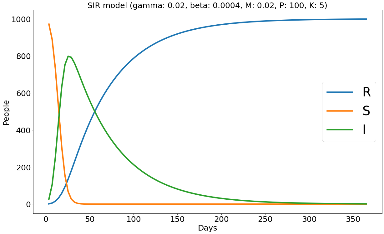
(a) Method #1 ($P=100,K=5$)

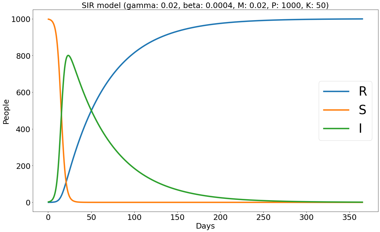
(b) Method #1 ($P=1000,K=50$)

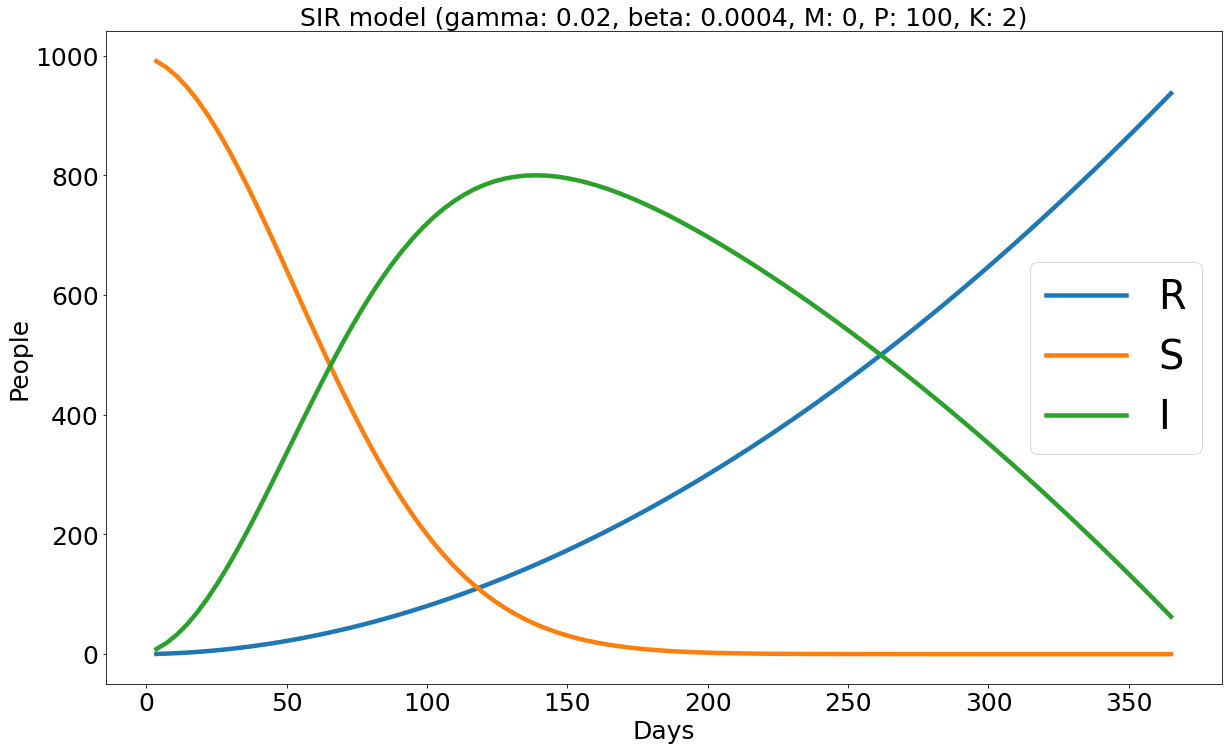
(c) Method #2 ($P=100,K=2$)

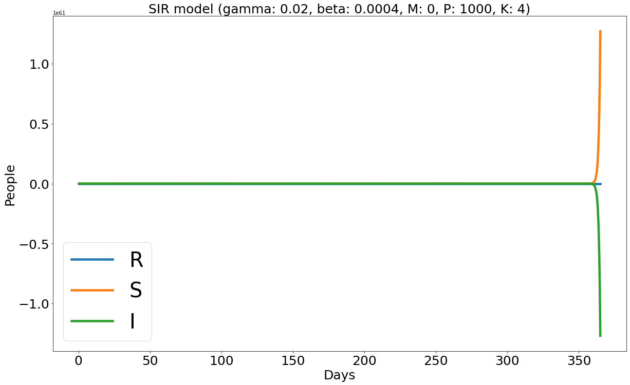
(d) Method #2 ($P=1000,K=4$)

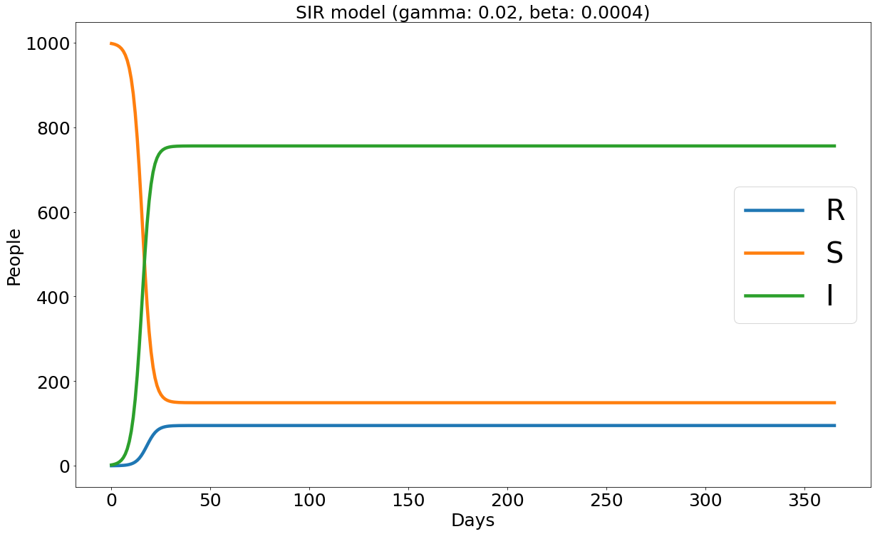
(e) Method #3

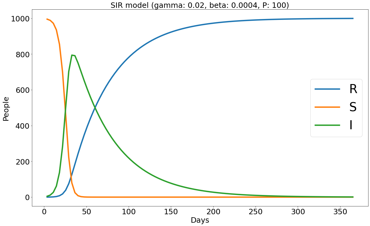
(f) Method #4 ($P=100$)

(g) Method #4 ($P=1000$)

Figure IV.1: Graphical illustrations of Test 1. Row 1: Euler-relaxation method. Row 2: regular linearization method. Row 3: approximate analytic method. Row 4: direct Euler method.

Test 2

Our second test focuses on the numerical comparison between two approaches: applying the well-known Runge-Kutta RK4 method (referred to as method #5) to our relaxation scheme (II.5) and applying it directly to the nonlinear differential equation (II.3) (denoted as method #6). Additionally, we compare the convergence speed of method #5 with method #1, referred above to as the Euler-relaxation method (II.8).

As RK4 is a fourth-order method, we deliberately choose a large population size of $N=97.47\times 10^{6}$ and a transmission rate of $\beta=3\times 10^{-9}$. Assuming the initial infected population is $a=11$, and the removal rate remains constant at $\gamma=0.05$ throughout the entire six-month period ($T=180$), we can calculate that the simulated disease reaches its peak at $I_{\max,\text{true}}=51367769$; cf. (II.4). Moreover, based on numerical observations with a sufficiently large value of $P$ (>2000), we find that this peak is reached on the 73rd day.

Our numerical results are tabulated in Table 2, accompanied by corresponding graphical illustrations in Figure IV.2. We see that within the same RK4 framework, our proposed relaxation method (method #5) outperforms the direct approach. When the number of time steps is small ($P=50$), method #5 with $K=20$ yields an amplitude $I_{\max}$ of 51295165 with a relative accuracy of 0.14%, while method #6 achieves 0.81%. Both methods capture the peak day (72) well compared to the true value of 73. Note in this case that we choose $K=20$, a larger value than in Test 1, due to the larger population under consideration. Cf. Theorem 3, the choice of $K$ does affect our error estimation which heavily depends on the total size of the removal population.

We also see that when increasing $P$ to 2000, our proposed method #5 with an increased $K=50$ precisely achieves the true amplitude, $I_{\max,\text{true}}=51367769$, while the direct RK4 method produces a very close approximation of 51367765. Both methods also identify the peak day as the 73rd day.

Furthermore, we compare our relaxation method to the Euler and Runge-Kutta frameworks. In terms of amplitude, although method #1 initially provides a better value of 51341234 with an accuracy of 0.05%, it fails to accurately detect the peak day, significantly deviating from the true value of 73 (predicting 54 instead). Increasing $P$ to 2000 improves the amplitude to 51367573, but it still performs worse than the direct RK4 method’s amplitude of 51367765. Herewith, method #1 achieves an improved peak day of 72. Additionally, based on the simulation of method #1, we observe that to reach the true amplitude ($I_{\max,\text{true}}=51367769$) and the true peak day of 73, at least $P=19000$ and $K=100$ are required. Henceforth, our relaxation method in the RK4 framework, as readily expected, outperforms itself in the Euler framework.

Method #	5	5	6	6	1	1
# of time step $P$	$50$	$2000$	$50$	$2000$	$50$	$2000$
# of iteration $K$	20	50	None	None	20	50
Amplitude $I_{\max}$	51295165	51367769	50948480	51367765	51341234	51367573
Peak day	72	73	72	73	54	72

Table 2: Values of the computed amplitude $I_{\max}$ obtained from different methods and the corresponding peak days. Method #5: our RK4-relaxation method (IV.3) applied with (IV.8)–(IV.12). Method #6: the conventional RK4 method (IV.3)–(IV.7) applied directly to the nonlinear differential equation (II.3). Method #1: our Euler-relaxation method (II.8). By (II.4), the true amplitude $I_{\max,\text{true}}$ is 51367769 in this scenario.

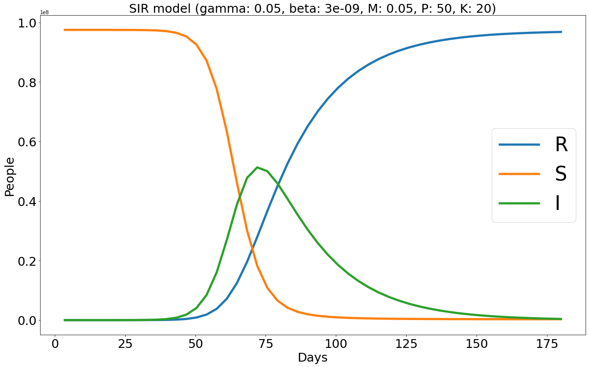
(a) Method #5 ($P=50,K=20$)

(b) Method #5 ($P=2000,K=50$)

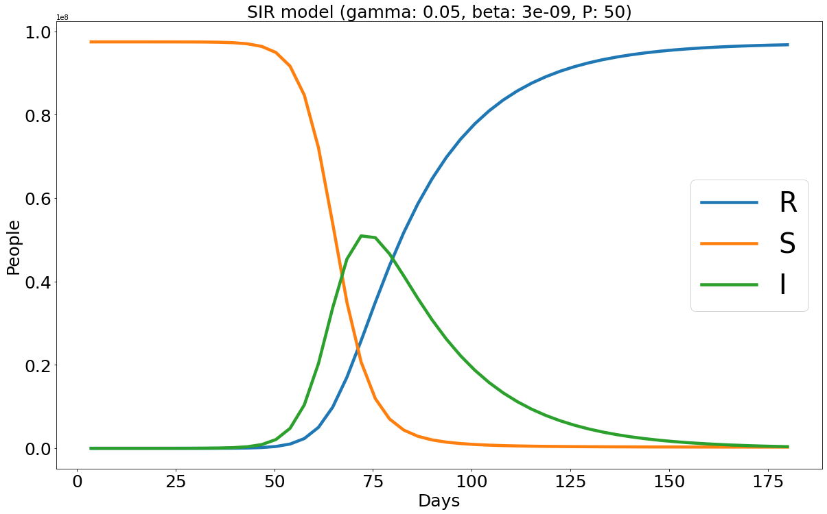
(c) Method #6 ($P=50$)

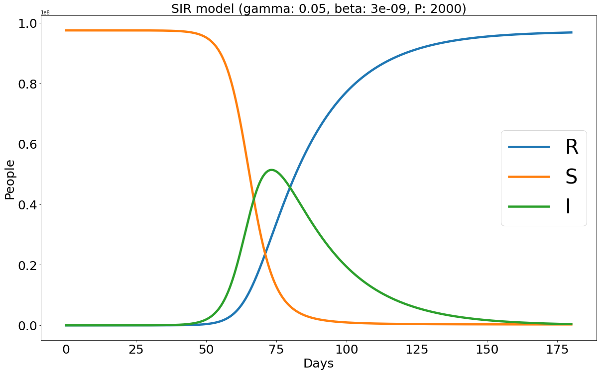
(d) Method #6 ($P=2000$)

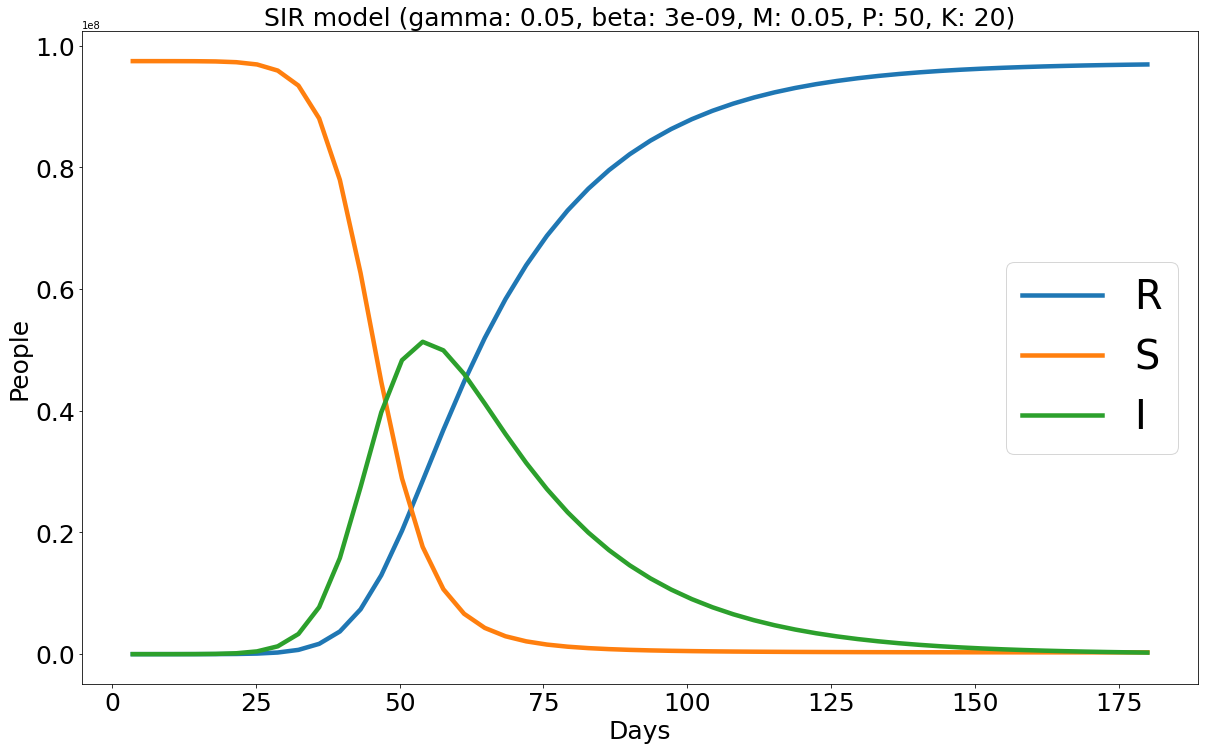
(e) Method #1 ($P=50,K=20$)

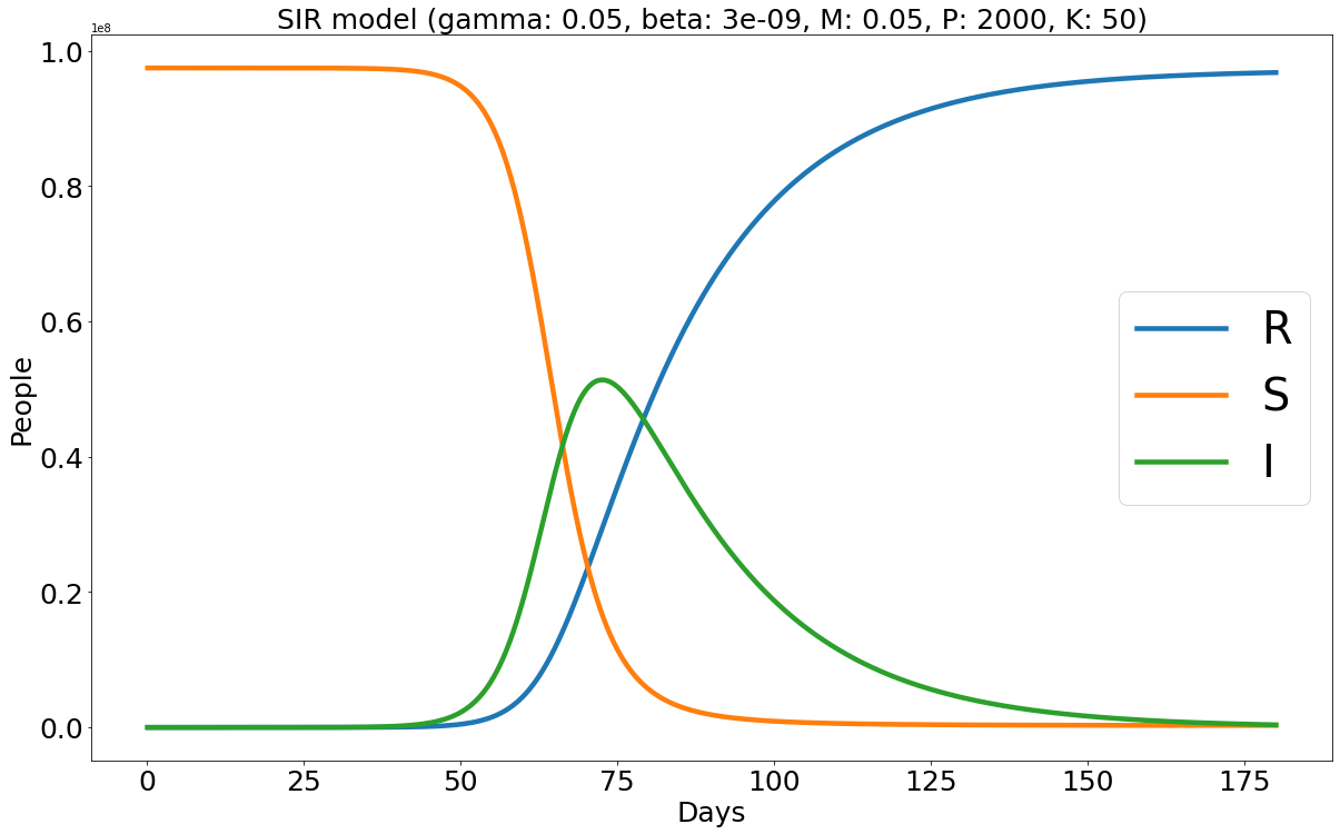
(f) Method #1 ($P=2000,K=50$)

Figure IV.2: Graphical illustrations of Test 2. Row 1: RK4-relaxation method. Row 2: direct RK4 method. Row 3: Euler-relaxation method.

Test 3

As previously mentioned, in our last experiment, we aim to broaden the scope of the proposed relaxation method by applying it to various SIR-type models: specifically, the SIRD model and the SIR model with background mortality. These models share the same input parameters as those used in Test 1, where we set $N=1000$, $n=998$, $T=365$, $\gamma=0.02$, $\beta=0.0004$. In the SIRD model (III.1), we choose a death rate of $\sigma=0.01$, which implies a choice of the relaxation parameter $\overline{M}\geq\gamma+\sigma=0.03$. In the SIR model with background mortality (III.7), we use the background death of $\sigma=0.001$ and select $\hat{M}\geq\gamma=0.02$.

Our numerical findings for the SIRD model are detailed in Figure IV.3. We specifically investigate the scenario where $\overline{M}=0.015$, thereby contravening the relaxation condition ($\overline{M}\geq 0.03$). Consistent with our theorem concerning non-negativity preservation, we observe that the relaxed solution with $\overline{M}=0.015$, obtained from both the Euler and RK4 frameworks, fails to maintain non-negativity over time. This is evident in the first column of Figure IV.3. When $\overline{M}=0.03$ (a case that adheres to the condition), we also note that the RK4-relaxation outperforms the Euler-relaxation approach. Given the $I_{\max,\text{true}}=730$ (as formulated in (III.2)), and with a coarse mesh of $P=200$ and $K=10$, we observe that the RK4-relaxation produces an amplitude identical to the true value. In contrast, the Euler-relaxation yields a value of 729. It is also worth mentioning that the accurate amplitude is attained when applying the Euler-relaxation with $P=800$ and $K=10$.

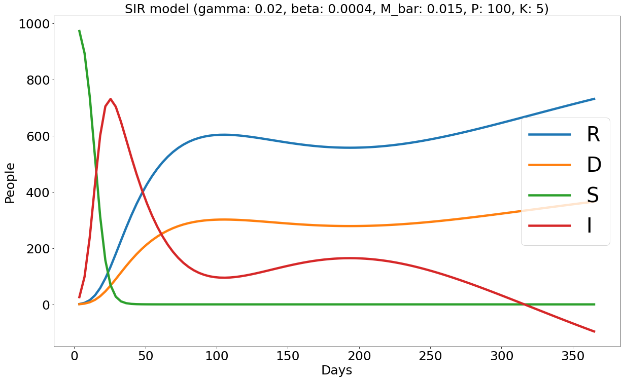
(a) Violating Euler-relaxation ($P=100,K=5$, $\overline{M}=0.015$)

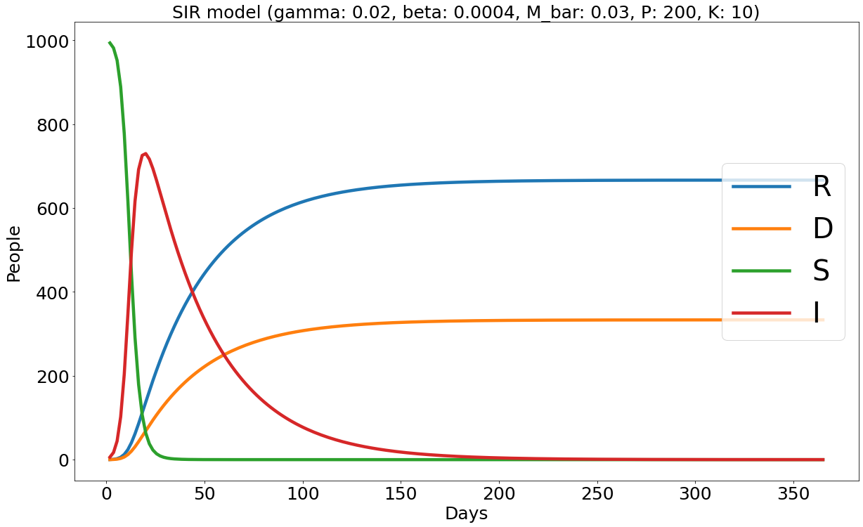
(b) Euler-relaxation ($P=200,K=10,\overline{M}=0.03$)

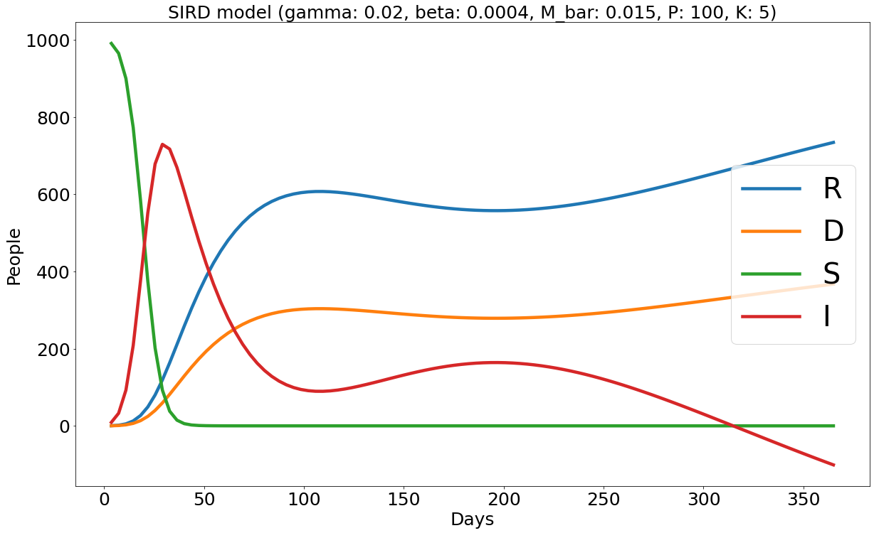
(c) Violating RK4-relaxation ($P=100,K=5,\overline{M}=0.015$)

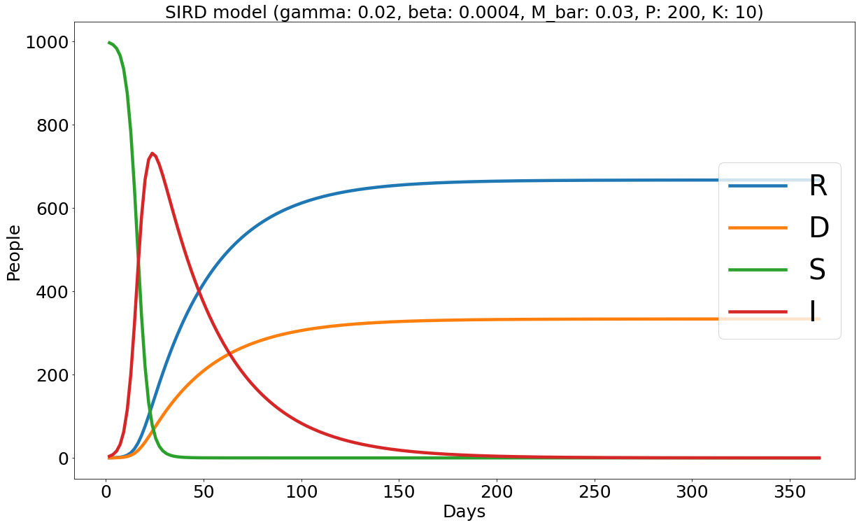
(d) RK4-relaxation ($P=200,K=10,\overline{M}=0.03$)

Figure IV.3: Graphical illustrations of Test 3 – SIRD model. Row 1: Euler-relaxation method with violating and non-violating cases. Row 2: RK4-relaxation method with violating and non-violating cases. These illustrations serve to highlight a crucial observation: when the relaxation parameter is not suitably selected, the numerical solution loses its adherence to non-negativity preservation.

Our numerical results pertaining to the SIR model with background mortality are presented in Figure IV.4. It is evident that both the Euler and RK4 relaxation methods show numerical stability and non-negativity preservation as we increase the values of $\left(P,K\right)$ from $\left(100,5\right)$ to $\left(1000,50\right)$.

Consistent with our prior tests, the RK4-relaxation method continues to outperform the Euler-relaxation method. Leveraging this numerical stability, we run the RK4-relaxation method using large values of $P$ and $K$ to determine the numerical amplitude and peak day. Our findings reveal a numerical amplitude of 777, peaking on the 24th day. Within the RK4 framework, achieving this numerical amplitude and peak day requires approximately $P=300$ and $K=20$. In contrast, the Euler framework demands a minimum of $P=1700$ and $K=20$ for similar outcomes.

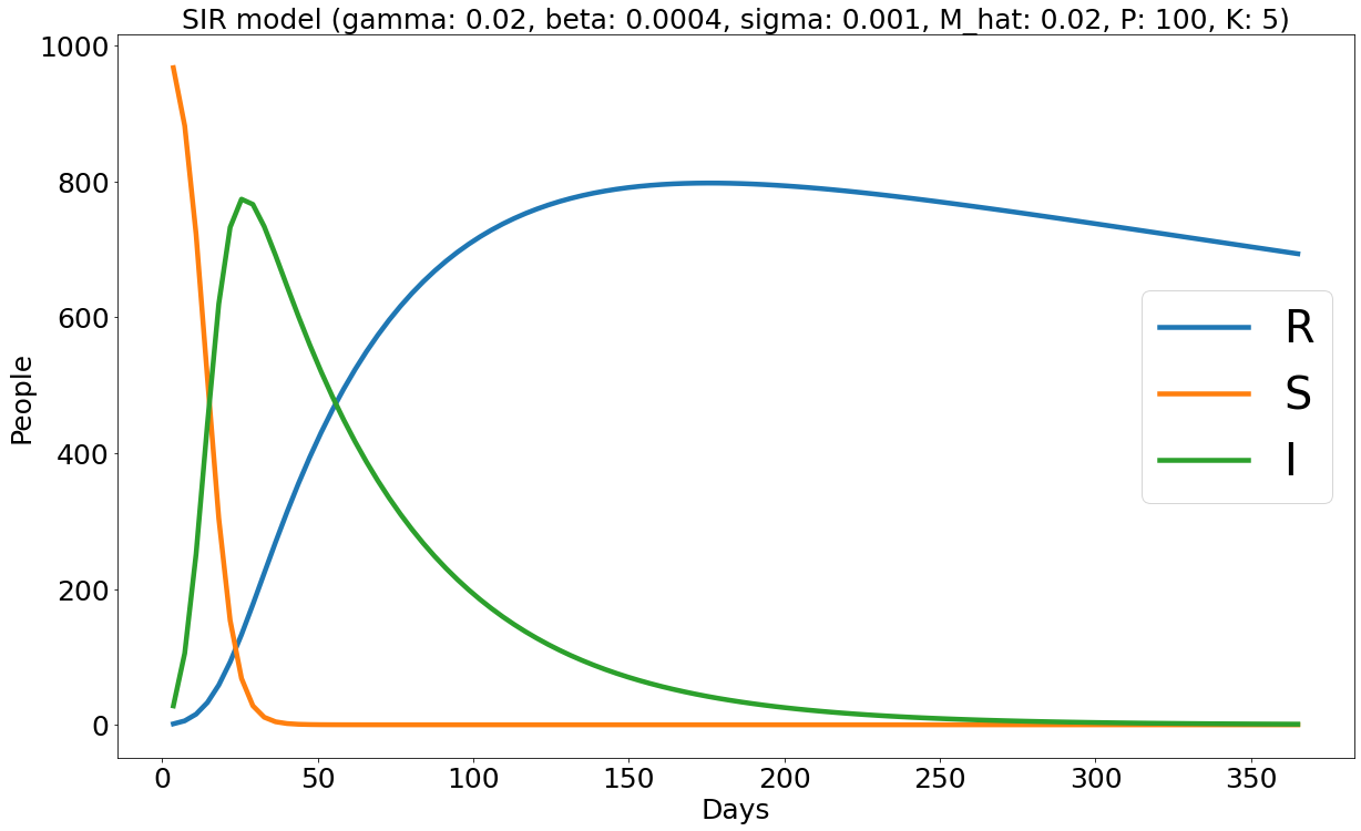
(a) Method #1 ($P=100,K=5$)

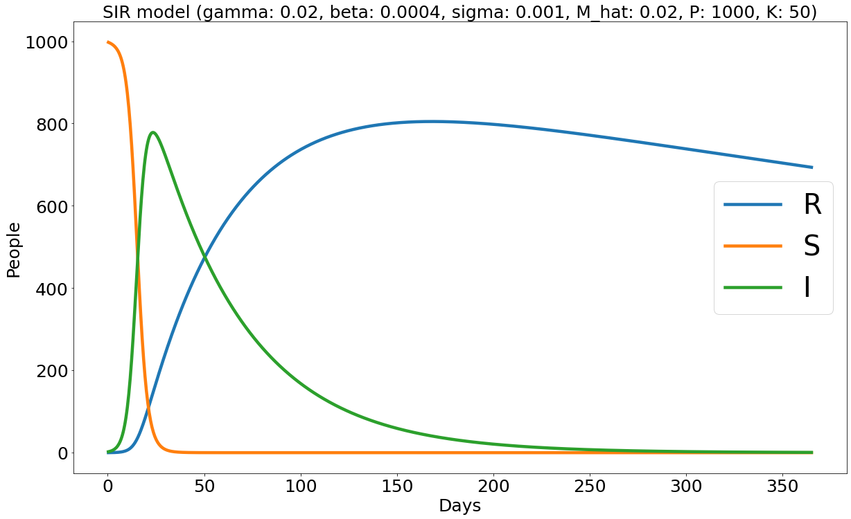
(b) Method #1 ($P=1000,K=50$)

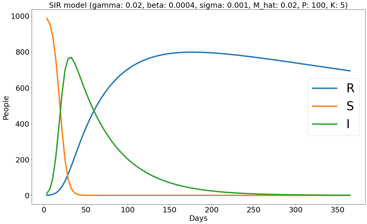
(c) Method #5 ($P=100,K=5$)

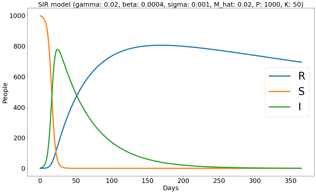
(d) Method #5 ($P=1000,K=50$)

Figure IV.4: Graphical illustrations of Test 3 – SIR model with background death. Row 1: Euler-relaxation method with different values of $P$ and $K$. Row 2: RK4-relaxation method with diverse $P$ and $K$ values. In these illustrations, numerical stability and non-negativity preservation are observed.

V Concluding remarks

This work presents a novel numerical approach for solving the SIR model in population dynamics. While various approximation methods have been proposed for this classical model, the analysis of their convergence has been limited and challenging. Our approach introduces the relaxation procedure to approximate the continuous model. By carefully selecting the relaxation parameter, we achieve global strong convergence of the scheme and effectively preserve non-negativity. The proposed scheme is explicit and straightforward to implement, enabling us to obtain the approximate solution at either the discrete or analytical level. Additionally, we showcase the applicability of our scheme to numerous variants of the SIR model.

In our future work, we aim to extend our method to a globally strongly convergent higher-order scheme. Furthermore, we plan to apply the method to more complex SIR-based models involving multiple compartments.

Credit authorship contribution statement

V. A. Khoa: Supervision, Conceptualization, Formal analysis, Writing–review & editing. P. M. Quan: Software, Visualization. K. W. Blayneh: Formal analysis, Writing–review & editing. J. Allen: Formal analysis, Visualization.

Declaration of competing interest

The authors declare that they have no known competing financial interests or personal relationships that could have appeared to influence the work reported in this paper.

Data availability

Simulated data will be made available on request.

Appendix

Proof of Theorem 3

Step 1: Define $\mathcal{E}_{k}\left(t\right)=R_{k}\left(t\right)-R\left(t\right)$ for $k=1,2,3,\ldots$. It follows from (II.5) and (II.3) that $\mathcal{E}_{k}$ satisfies the following differential equation:

$$\mathcal{E}_{k}^{\prime}\left(t\right)+M\mathcal{E}_{k}\left(t\right) =-g\left(R_{k-1}\left(t\right)\right)+g\left(R\left(t\right)\right)+M\mathcal{E}_{k-1}\left(t\right)$$

$$=p\left(R\left(t\right)\right)-p\left(R_{k-1}\left(t\right)\right),$$ (V.1)

where we have denoted $p\left(r\right)=g\left(r\right)-Mr$ for $r\geq 0$. Herewith, by Theorems 1 and 2, we are allowed to consider $r\geq 0$. We can compute that $p^{\prime}\left(r\right)=-\gamma n\mu e^{-\mu r}+\gamma-M$. Then, for $M\geq\gamma$ and since $r\geq 0$, we estimate that

$$\gamma-\gamma n\mu-M\leq p^{\prime}\left(r\right)=-\gamma n\mu e^{-\mu r}+\gamma-M<0,$$

which shows

$$\left|p^{\prime}\left(r\right)\right|\leq M+\gamma n\mu-\gamma.$$ (V.2)

Therefore, the left-hand side of (V.1) can be bounded from above by

$$\mathcal{E}_{k}^{\prime}\left(t\right)+M\mathcal{E}_{k}\left(t\right)\leq\left(M+\gamma n\mu-\gamma\right)\left|\mathcal{E}_{k-1}\left(t\right)\right|.$$

Using the Hölder inequality, we find that

$$e^{2Mt}\left|\mathcal{E}_{k}\left(t\right)\right|^{2} \leq\left(M+\gamma n\mu-\gamma\right)^{2}\left(\int_{0}^{t}e^{Ms}\left|\mathcal{E}_{k-1}\left(s\right)\right|ds\right)^{2}$$

$$\leq\left(M+\gamma n\mu-\gamma\right)^{2}\int_{0}^{t}e^{2Ms}ds\int_{0}^{t}\left|\mathcal{E}_{k-1}\left(s\right)\right|^{2}ds.$$

Thus, we deduce that

$$\left|\mathcal{E}_{k}\left(t\right)\right|^{2}\leq\frac{1}{2M}\left(M+\gamma n\mu-\gamma\right)^{2}\left(1-e^{-2Mt}\right)\int_{0}^{t}\left|\mathcal{E}_{k-1}\left(s\right)\right|^{2}ds.$$

By the elementary inequality $e^{-x}+x\geq 1$, we obtain the following estimate

$$\left|\mathcal{E}_{k}\left(t\right)\right|^{2}\leq\left(M+\gamma n\mu-\gamma\right)^{2}t\int_{0}^{t}\left|\mathcal{E}_{k-1}\left(s\right)\right|^{2}ds.$$ (V.3)

Step 2: By induction, we can show that for any $2\leq k\in\mathbb{N}$

$$\left|\mathcal{E}_{k}\left(t\right)\right|^{2}\leq\left(M+\gamma n\mu-\gamma\right)^{2k}t\int_{0}^{t}s_{1}\int_{0}^{s_{1}}\ldots s_{k-1}\int_{0}^{s_{k-1}}\left|\mathcal{E}_{0}\left(s_{k}\right)\right|^{2}ds_{k}ds_{k-1}\ldots ds_{1}$$ (V.4)

It follows from (V.3) that (V.4) holds true for $k=2$. Indeed,

$$\left|\mathcal{E}_{2}\left(t\right)\right|^{2}\leq\left(M+\gamma n\mu-\gamma\right)^{2}t\int_{0}^{t}\left|\mathcal{E}_{1}\left(s_{1}\right)\right|^{2}ds_{1}\leq\left(M+\gamma n\mu-\gamma\right)^{4}t\int_{0}^{t}s_{1}\int_{0}^{s_{1}}\left|\mathcal{E}_{0}\left(s_{2}\right)\right|^{2}ds_{2}ds_{1}.$$

Assume that (V.4) holds true for $k=k_{0}$. We show that it also holds true for $k=k_{0}+1$. By (V.3), we have

$$\left|\mathcal{E}_{k_{0}+1}\left(t\right)\right|^{2}$$

$$\leq\left(M+\gamma n\mu-\gamma\right)^{2}t\int_{0}^{t}\left|\mathcal{E}_{k_{0}}\left(s\right)\right|^{2}ds$$

$$\leq\left(M+\gamma n\mu-\gamma\right)^{2}t\int_{0}^{t}\left(M+\gamma n\mu-\gamma\right)^{2k_{0}}s\int_{0}^{s}s_{1}\int_{0}^{s_{1}}\ldots s_{k_{0}-1}\int_{0}^{s_{k_{0}-1}}\left|\mathcal{E}_{0}\left(s_{k_{0}}\right)\right|^{2}ds_{k_{0}}ds_{k_{0}-1}\ldots ds_{1}ds$$

$$\leq\left(M+\gamma n\mu-\gamma\right)^{2\left(k_{0}+1\right)}\int_{0}^{t}s_{1}\int_{0}^{s_{1}}\ldots s_{k_{0}}\int_{0}^{s_{k_{0}}}\left|\mathcal{E}_{0}\left(s_{k_{0}+1}\right)\right|^{2}ds_{k_{0}+1}ds_{k_{0}}\ldots ds_{1}.$$

Hence, we complete Step 2.

Step 3: By (V.4), observe that $0\leq s_{k}\leq s_{k-1}\leq\ldots\leq s_{1}\leq t$. Combining this, (V.4) and the fact that $R\in C^{1}$ gives

$$\left|\mathcal{E}_{k}\left(t\right)\right|^{2} \leq\left(M+\gamma n\mu-\gamma\right)^{2k}t^{k+1}\max_{0\leq t\leq T}\left|\mathcal{E}_{0}\left(t\right)\right|^{2}\int_{0}^{t}s_{1}\int_{0}^{s_{1}}\ldots s_{k-1}\int_{0}^{s_{k-1}}ds_{k}ds_{k-1}\ldots ds_{1}$$

$$\leq\left(M+\gamma n\mu-\gamma\right)^{2k}\frac{t^{k+1}}{k!}\max_{0\leq t\leq T}\left|\mathcal{E}_{0}\left(t\right)\right|^{2}.$$

Note that we have the $k$ and time independence of $M+\gamma n\mu-\gamma$ and $t\leq T$. Moreover, we know that $\mathcal{E}_{0}\left(t\right)=R_{0}\left(t\right)-R\left(t\right)=-R\left(t\right)$ by the choice $R_{0}\left(t\right)=0$. Therefore, in view of the fact that $\lim_{k\to\infty}\frac{Q^{k}}{k!}=0$ for any constant $Q>0$, we can always find $\overline{k}>0$ such that for any $k\geq\overline{k}$,

$$\left(M+\gamma n\mu-\gamma\right)^{2k}\frac{T^{k+1}}{k!}<1.$$

Hence, we obtain the strong convergence of the sequence $\left\{R_{k}\right\}_{k=0}^{\infty}$ toward the true solution $R$.

Proof of Corollary 4

We define $\mathcal{E}_{k}\left(t\right)=R_{k}\left(t\right)-R\left(t\right)$ and $p\left(r\right)=g\left(r\right)-Mr$ as above. Multiplying (V.1) by $\mathcal{E}_{k}\left(t\right)$ and using (V.2) yield

$$\frac{1}{2}\frac{d}{dt}\mathcal{E}_{k}^{2}\left(t\right)+M\mathcal{E}_{k}^{2}\left(t\right)=\left[p\left(R\left(t\right)\right)-p\left(R_{k-1}\left(t\right)\right)\right]\mathcal{E}_{k}\left(t\right)\leq\frac{M+\gamma n\mu-\gamma}{2}\mathcal{E}_{k-1}^{2}\left(t\right)+\frac{M+\gamma n\mu-\gamma}{2}\mathcal{E}_{k}^{2}\left(t\right).$$

Equivalently, we obtain

$$\frac{d}{dt}\mathcal{E}_{k}^{2}\left(t\right)+\left(M-\gamma n\mu+\gamma\right)\mathcal{E}_{k}^{2}\left(t\right)\leq\left(M+\gamma n\mu-\gamma\right)\mathcal{E}_{k-1}^{2}\left(t\right).$$

Notice that by the choice $M\geq\gamma$, it holds true that $M>\gamma n\mu-\gamma$ when $n\mu<1$. Using the integrating factor $e^{\left(M-\gamma n\mu+\gamma\right)t}$ and taking integration with respect to $t$, we get

$$\mathcal{E}_{k}^{2}\left(t\right) \leq e^{-\left(M-\gamma n\mu+\gamma\right)t}\left(M+\gamma n\mu-\gamma\right)\int_{0}^{t}e^{\left(M-\gamma n\mu+\gamma\right)s}\mathcal{E}_{k-1}^{2}\left(s\right)ds$$

$$\leq e^{-\left(M-\gamma n\mu+\gamma\right)t}\left[e^{\left(M-\gamma n\mu+\gamma\right)t}-1\right]\frac{M+\gamma n\mu-\gamma}{M-\gamma n\mu+\gamma}\max_{0\leq t\leq T}\mathcal{E}_{k-1}^{2}\left(t\right).$$

Henceforth, we obtain

$$\max_{0\leq t\leq T}\left|\mathcal{E}_{k}\left(t\right)\right|\leq\left(\frac{M+\gamma n\mu-\gamma}{M-\gamma n\mu+\gamma}\right)^{1/2}\max_{0\leq t\leq T}\left|\mathcal{E}_{k-1}\left(t\right)\right|.$$ (V.5)

By induction and the fact that $R_{0}\left(t\right)=0$, we deduce

$$\max_{0\leq t\leq T}\left|\mathcal{E}_{k}\left(t\right)\right|\leq\left(\frac{M+\gamma n\mu-\gamma}{M-\gamma n\mu+\gamma}\right)^{k/2}\max_{0\leq t\leq T}\left|\mathcal{E}_{0}\left(t\right)\right|=\left(\frac{M+\gamma n\mu-\gamma}{M-\gamma n\mu+\gamma}\right)^{k/2}\max_{0\leq t\leq T}\left|R\left(t\right)\right|.$$

Since $M+\gamma n\mu-\gamma<M-\gamma n\mu+\gamma$ when $n\mu<1$, we obtain the target estimate (II.6).

References

- [1] N. T. J. Bailey. The mathematical theory of infectious diseases and its applications. Griffin, 1975.
- [2] N. S. Barlow and S. J. Weinstein. Accurate closed-form solution of the SIR epidemic model. Physica D: Nonlinear Phenomena, 408:132540, 2020.
- [3] G. Bärwolff. Modeling of COVID-19 propagation with compartment models. Mathematische Semesterberichte, 68(2):181–219, 2021.
- [4] J. Caldwell and D. K. S. Ng. Mathematical Modelling: Case Studies and Projects. Springer, 2004.
- [5] Y. Chakir. Global approximate solution of SIR epidemic model with constant vaccination strategy. Chaos, Solitons & Fractals, 169:113323, 2023.
- [6] D. Conte, N. Guarinoa, G. Paganoa, and B. Paternoster. Positivity-preserving and elementary stable nonstandard methodfor a COVID-19 SIR model. Dolomites Research Notes on Approximation, 15:65–77, 2022.
- [7] D. J. D. Earn, J. Dushoff, and S. A. Levin. Ecology and evolution of the flu. Trends in Ecology & Evolution, 17(7):334–340, 2002.
- [8] E. Hairer, S. P. Nørsett, and G. Wanner. Solving Ordinary Differential Equations I: Nonstiff Problems. Springer Berlin Heidelberg, 2008.
- [9] T. Harko, F. S. N. Lobo, and M. K. Mak. Exact analytical solutions of the Susceptible-Infected-Recovered (SIR) epidemic model and of the SIR model with equal death and birth rates. Applied Mathematics and Computation, 236:184–194, 2014.
- [10] W. O. Kermack and A. G. McKendrick. A contribution to the mathematical theory of epidemics. Proceedings of the Royal Society of London. Series A, Containing Papers of a Mathematical and Physical Character, 115(772):700–721, 1927.
- [11] A. Khaleque and P. Sen. An empirical analysis of the Ebola outbreak in West Africa. Scientific Reports, 7(1), 2017.
- [12] M. M. Khalsaraei, A. Shokri, H. Ramos, and S. Heydari. A positive and elementary stable nonstandard explicit scheme for a mathematical model of the influenza disease. Mathematics and Computers in Simulation, 182:397–410, 2021.
- [13] V. A. Khoa, E. R. Ijioma, and N. N. Ngoc. Strong convergence of a linearization method for semi-linear elliptic equations with variable scaled production. Computational and Applied Mathematics, 39(4), 2020.
- [14] V. A. Khoa, E. R. Ijioma, and N. N. Ngoc. Correction to: Strong convergence of a linearization method for semi-linear elliptic equations with variable scaled production. Computational and Applied Mathematics, 40(1), 2021.
- [15] N. A. Kudryashov, M. A. Chmykhov, and M. Vigdorowitsch. Analytical features of the SIR model and their applications to COVID-19. Applied Mathematical Modelling, 90:466–473, 2021.
- [16] B. F. Maier and D. Brockmann. Effective containment explains subexponential growth in recent confirmed COVID-19 cases in China. Science, 368(6492):742–746, 2020.
- [17] O. D. Makinde. Adomian decomposition approach to a SIR epidemic model with constant vaccination strategy. Applied Mathematics and Computation, 184(2):842–848, 2007.
- [18] R. E. Mickens. Numerical integration of population models satisfying conservation laws: NSFD methods. Journal of Biological Dynamics, 1(4):427–436, 2007.
- [19] K. Mitra and I. S. Pop. A modified L-scheme to solve nonlinear diffusion problems. Computers & Mathematics with Applications, 77(6):1722–1738, 2019.
- [20] W. Piyawong, E. H. Twizell, and A. B. Gumel. An unconditionally convergent finite-difference scheme for the SIR model. Applied Mathematics and Computation, 146(2-3):611–625, 2003.
- [21] D. Prodanov. Comments on some analytical and numerical aspects of the SIR model. Applied Mathematical Modelling, 95:236–243, 2021.
- [22] D. Prodanov. Asymptotic analysis of the SIR model and the Gompertz distribution. Journal of Computational and Applied Mathematics, 422:114901, 2023.
- [23] S. Side, A. M. Utami, Sukarna, and M. I. Pratama. Numerical solution of SIR model for transmission of tuberculosis by Runge-Kutta method. Journal of Physics: Conference Series, 1040:012021, 2018.
- [24] T. C. Sideris. Ordinary Differential Equations and Dynamical Systems. Atlantis Press, 2013.
- [25] M. Slodicka. Error estimates of an efficient linearization scheme for a nonlinear elliptic problem with a nonlocal boundary condition. ESAIM: Mathematical Modelling and Numerical Analysis, 35(4):691–711, 2001.