A New Heterogeneous Hybrid Massive MIMO Receive Structure of Rapidly Eliminating DOA Ambiguity via Machine Learning

Abstract

Massive multiple input multiple output(MIMO)-based fully-digital receive antenna arrays eventuate a huge amount of circuit costs and complexity to direction of arrival(DOA) estimation, which is hard to satisfy the needs of high precision and low cost in future green wireless communication. To address this challenge, a novel heterogeneous hybrid MIMO receiver is proposed in this paper and a high performance DOA estimator called heterogeneous cross-minimum distance (HCMD) is developed based on the structure. The antenna arrays are first divided into multiple groups, and each group adopts a different hybrid structure. The virtual antenna arrays of these groups are then used for DOA estimation to generate multiple candidate angle sets, where each set contains a unique true solution and multiple pseudo-solutions. Finally, the cross-distance minimization method is applied to the multiple candidate angle sets to select the corresponding true solution for each group, and the final DOA estimation is given by combining the multiple true solutions. Simulation results show that as the number of antennas tends to large-scale, the proposed method can rapidly find the true solution for each group and achieve excellent estimation performance.

I Introduction

Target localization is a well attended issue in wireless communication research and is widely used in many fields, which mainly includes the techniques of time of arrival (TOA), received signal strength (RSS) and angle of arrival (AOA)[1, 2, 3, 4]. In particular, the authors discussed a methodology to achieve optimal geometric configurations under regional constraints for the RSS-based localization problem of Unmanned Aerial Vehicles (UAVs) in [5]. Direction of Arrival (DOA) technique as a key part of target localization, which can provide precise desired signal direction for beam forming and tracking[6]. In recent years, the emergence of Multiple Input Multiple Output (MIMO) technology in combination with DOA can achieve ultra-high angular resolution, but on the contrary, it brings a significantly higher RF-chain circuit cost and computational complexity.

To solve this challenge, adopting low-resolution ADCs is a promising solution. Low-resolution ADCs could save considerable circuit cost and power consumption. There are many existed works about low-resolution ADCs, like one-bit ADC, low-resolution ADC structure, mixed-ADC structure, and so on [7, 8, 9, 10, 11].

HAD structure connect one radio frequency (RF) chain with multi antennas. Every antenna has a analog phase shifter. Then the signals from multi antennas are added and converted to the baseband signals by one RF chain. authors proposed a low-complexity HAD structure and three corresponding methods in [12] to achieve high-precision and low-time-slot DOA estimation. To reduce the time blocks required for ambiguity elimination, a fast structure of removing spurious direction angles was proposed in [13], which can eliminate the phase ambiguity using two time slots. In addition, the authors proposed a deep learning based low complexity MIMO estimator for uniform circular arrays (UCA) in [14]. The feature information of the received signal is trained and predicted by deep learning to get the coarse DOA estimation, followed by maximum likelihood method to search for the optimal solution in a small range.

In general, how to utilize the massive HAD structure to eliminate the phase ambiguity rapidly and achieve high performance DOA estimation is a challenge to be solved. In this paper, we divide the massive HAD receiver arrays into several heterogeneous groups and get the final DOA estimation by special internal structure.

Notations: In this paper, signs $(\cdot)^{T}$, $(\cdot)^{H}$, $|\cdot|$ and $\|\cdot\|$ represent transpose, conjugate transpose, modulus and norm, respectively. $\mathbf{x}$ and $\mathbf{X}$ in bold typeface are used to represent vectors and matrices, respectively, while scalars are presented in normal typeface, such as $x$. $\mathbf{I}_{M}$ represents the $M\times M$ identity matrix, $\mathbf{0}_{a\times b}$ denotes the $a\times b$ matrix of all zeros and $\mathbf{1}_{M}$ denotes the $M\times 1$ vector of all $1$. Furthermore, $\mathbb{E}[\cdot]$ and $\mathbb{R}[\cdot]$ denotes the expectation operator and the real part of a complex-valued number, respectively. $\otimes$ denotes the Kronecker product. $\mathbf{diag}(\mathbf{X})$ and $\mathbf{Diag}(\mathbf{x})$ represent a diagonal matrix by keeping only the diagonal elements of matrix $\mathbf{X}$ and a diagonal matrix composed of $\mathbf{x}$. $\mathbf{Tr}(\cdot)$ and $\lceil\cdot\rceil$ respectively denote the matrix trace and the round up operation.

II System model

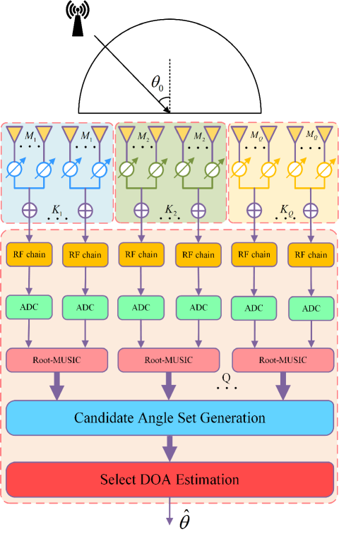
Figure 1: Proposed a new heterogeneous hybrid structure for massive MIMO with ULA

Fig. 1 shows the proposed heterogeneous hybrid structure. Consider a far-field narrowband signal $s(t)e^{j2\pi f_{c}t}$ impinge on the hybrid analog and digital (HAD) antenna array, where $s(t)$ is the baseband signal, and $f_{c}$ is the carrier frequency. We assume a uniform linear array (ULA) with the $M$ antennas which is divided into $Q$ groups, each group has $N_{q}$ antennas and consists of $K_{q}$ subarrays. In addition, each subarray contains $M_{q}$ antennas, i.e.,

$$M=\sum_{q=1}^{Q}N_{q}=\sum_{q=1}^{Q}K_{q}M_{q},~{}q=1,2,\cdots,Q$$ (1)

In special cases, when $M_{1}=M_{2}=,\cdots,M_{Q}$, this array can be represented as a common sub-connected hybrid architectures. In the $q$th group, the received signal at the $m$-th antenna of the $k$-th subarray is expressed as

$$x_{q,k,m}(t)=s(t)e^{j2\pi(f_{c}t-f_{c}\tau_{q,k,m})}+w_{q,k,m}(t),$$ (2)

where $w_{q,k,m}(t)\sim\mathcal{C}\mathcal{N}(0,\sigma^{2}_{w})$ is the additive white Gaussian noise (AWGN) vector, and $\tau_{q,k,m}$ are the propagation delays determined by the direction of the source relative to the array given by

$$\tau_{q,k,m}=\tau_{0}-\frac{d_{m}\sin\theta_{0}}{c},$$ (3)

where $\tau_{0}$ is the propagation delay from the emitter to a reference point on the array, $c$ is the speed of light, and $d_{m}$ denotes the distance from a common reference point to the $m$ th antenna of the $k$th subarray. Since we choose the left of the array as the reference point in this paper, the $d_{m}=(km-1)d$. Assuming $\phi_{q,k,m}$ be the corresponding phase for analog beamforming corresponding to the $k$-th RF chain and the $m$-th antenna $(m=1,2,\cdots,M_{q})$, then the output signal of the $k$th subarray is

$$y_{q,k}(t)=\frac{1}{\sqrt{M_{q}}}\sum_{m=1}^{M_{q}}x_{q,k,m}(t)e^{-j\phi_{q,k,m}}+w_{q,k}(t),$$ (4)

Stacking all $K_{q}$ subarray outputs and passes through parallel RF chains, the baseband signal vector of $q$th group is formed by

$$\mathbf{y}_{q}(t)=\mathbf{B}_{A,q}^{H}\mathbf{a}(\theta_{0})s(t)+\mathbf{w}(t),$$ (5)

where $\mathbf{w}(t)=\left[w_{1}(t),w_{2}(t),\ldots,w_{N_{q}}(t)\right]^{T}\in\mathbb{C}^{N_{q}\times 1}$ is the AWGN vector, $\mathbf{B}_{A,q}$ is a block diagonal matrix, whose $k$-th block diagonal element can be represented as

$$\mathbf{b}_{A,q,k}=\frac{1}{\sqrt{M_{q}}}\left[e^{j\phi_{k,1}},e^{j\phi_{k,2}},\cdots,e^{j\phi_{k,M_{q}}}\right]^{T},$$ (6)

and the vector $\mathbf{a}_{q}(\theta_{0})\in\mathbb{C}^{N_{q}\times 1}$ is the array manifold defined as

$$\mathbf{a}_{q}\left(\theta_{0}\right)=\left[1,e^{j\frac{2\pi}{\lambda}d\sin\theta_{0}},\cdots,e^{j\frac{2\pi}{\lambda}(N_{q}-1)d\sin\theta_{0}}\right]^{T},$$ (7)

Via analog-to-digital convertor (ADC) and digital beamforming (DB), the (5) can be further expressed as

$$\mathbf{r}_{q}(n)=\mathbf{b}_{D}^{H}\mathbf{B}_{A,q}^{H}\mathbf{a}_{q}(\theta_{0})s(n)+\mathbf{b}_{D}^{H}\mathbf{w}(n),$$ (8)

where $n=1,2,\cdots,N$, $N$ is the number of snapshots, $\mathbf{b}_{D}$ is the DB vector and defined $\mathbf{b}_{D}=\left[b_{1},b_{2},\cdots,b_{K_{q}}\right]^{T}$.

III Proposed high-performance HCMD DOA estimator

In this section, to rapidly eliminate the pseudo-solutions and get the correct direction, a high-performance DOA estimator based on heterogeneous hybrid structure called HCMD are proposed and the corresponding error lower bound is derived.

Through the above discussion, each sub-array in the $q$th group is seem as a virtual antenna. Assume that the analog beamforming vector $\mathbf{b}_{A,q,k}=\frac{1}{M_{q}}[1,\cdots,1]^{T}$, the output vector of $K_{q}$ subarrays is

$$\mathbf{y}_{q}(n) =[y_{1}(n),y_{2}(n),\cdots,y_{K_{q}}(n)]^{T}$$ (9)

$$=\frac{1}{M_{q}}\mathbf{a}_{M_{q}}(\theta_{0})g_{q}(\theta_{0})s(n)+[w_{1}^{b}(n),\cdots,w_{K_{q}}]^{T},$$

where $\mathbf{a}_{M_{q}}$ is the array manifold vector of the virtual array, which can be defined as

$$\mathbf{a}_{M_{q}}\left(\theta_{0}\right)=\left[1,e^{j\frac{2\pi}{\lambda}M_{q}d\sin\theta_{0}},\cdots,e^{j\frac{2\pi}{\lambda}(K_{q}-1)M_{q}d\sin\theta_{0}}\right]^{T},$$ (10)

and $g_{q}(\theta_{0})$ is a constant given by summing all elements of each subarray can be denotes as

$$g_{q}\left(\theta_{0}\right) =\sum_{m=1}^{M_{q}}e^{j\frac{2\pi}{\lambda}(m-1)d\sin\theta_{0}}$$ (11)

$$=\frac{1-e^{j\frac{2\pi}{\lambda}M_{q}d\sin\theta_{0}}}{1-e^{j\frac{2\pi}{\lambda}d\sin\theta_{0}}}$$

Based on (9), the covariance matrix of the output vector $\mathbf{y_{q}(n)}$ of the virtual antenna array is

$$\mathbf{R}_{q} =\mathbb{E}\left[\mathbf{y_{q}}(n)\mathbf{y_{q}}(n)^{H}\right]$$ (12)

$$=\frac{1}{M_{q}}\sigma_{s}^{2}\left\|g_{q}\left(\theta_{0}\right)\right\|^{2}\mathbf{a}_{M_{q}}\left(\theta_{0}\right)\mathbf{a}_{M_{q}}^{H}\left(\theta_{0}\right)+\sigma_{w}^{2}\mathbf{I},$$ (13)

where $\sigma_{s}^{2}$ represents the variance of the receive signal. Furthermore, the eigenvalue decomposition (EVD) of $\mathbf{R}_{q}$ is expressed as

$$\mathbf{R}_{q} =\mathbf{U}\Sigma\mathbf{U}^{H}=[\mathbf{U}_{S}\mathbf{U}_{N}]\Sigma[\mathbf{U}_{S}\mathbf{U}_{N}]^{H},$$ (14)

where $\mathbf{U}_{S}$ and $\mathbf{U}_{N}$ stand for the signal and noise subspaces, respectively. The $K_{q}\times K_{q}$ diagonal matrix has the following form

$$\Sigma=\left[\begin{array}[]{cccc}\sigma_{s}^{2}+\sigma_{w}^{2}&0&\cdots&0\\ 0&\sigma_{w}^{2}&\cdots&0\\ \vdots&\vdots&\ddots&\vdots\\ 0&0&\cdots&\sigma_{w}^{2}\end{array}\right].$$ (19)

Then, the pseudo spectrum corresponding to the virtual antenna array can be given by

$$P_{RM}(\theta)=\frac{1}{\left\|\mathbf{U}_{N}^{H}\mathbf{a}_{M_{q}}(\theta)g_{q}(\theta)\right\|^{2}},$$ (20)

which spectral peak corresponds to the desire DOA estimation and the Root-MUSIC [15] is reliable due to its low-complexity and excellent asymptotic performance. Furthermore, let us define $\mathbf{V}=\mathbf{U}_{N}\mathbf{U}_{N}^{H}$, the polynomial equation can be expressed as

$$p(\theta) =g_{q}^{H}(\theta)\mathbf{a}_{M_{q}}^{H}(\theta)\mathbf{U}_{N}\mathbf{U}_{N}^{H}\mathbf{a}_{M_{q}}(\theta)g_{q}(\theta)\triangleq p(z)$$ (21)

$$=\frac{2-z^{-1}-z}{2-z^{-\frac{1}{M_{q}}}-z^{\frac{1}{M_{q}}}}\sum_{i=1}^{K_{q}}\sum_{j=1}^{K_{q}}z^{-(i-1)}\mathbf{V}_{ij}z^{j-1}=0,$$

where $\mathbf{V}_{ij}$ is the element in the $i$th column of the $j$th row of $\mathbf{V}$ and

$$z=e^{j\xi_{q}},$$ (22)

where $\xi_{q}=2\pi M_{q}dsin\theta/\lambda$. The above polynomial equation (21) has $2K_{q}-2$ roots, i.e $z_{i},i=1,\cdots,2K_{q}-2$, which implies the existence of multiple emitter directions as follows

$$\hat{\Theta}_{RM}=\left\{\hat{\theta}_{i},i\in\{1,2,\cdots,2K_{q}-2\}\right\},$$ (23)

where

$$\hat{\theta}_{i}=\arcsin\left(\frac{\lambda\arg z_{i}}{2\pi M_{q}d}\right)$$ (24)

Then, the angle corresponding to the nearest root to the unit circle is selected as the DOA estimation $\theta_{q}$ of $q$th array group and

$$\hat{\xi}_{q}=\frac{2\pi}{\lambda}M_{q}dsin\theta_{q}$$ (25)

Since each virtual antenna corresponds to a subarray, there exists phase ambiguity that needs to be eliminated, which can be expressed as

$$p(\hat{\xi}_{q})=p(\hat{\xi}_{q}+2\pi j)$$ (26)

Therefore, a feasible set containing $M_{q}$ solutions as follows

$$\hat{\Theta}_{q}=\left\{\hat{\theta}_{q,j},j\in\{1,2,\cdots,M_{q}\}\right\}$$ (27)

where

$$\hat{\theta}_{q,j}=\arcsin\left(\frac{\lambda\left(\arg(e^{j\hat{\xi}_{q}})+2\pi j\right)}{2\pi M_{q}d}\right).$$ (28)

Combing all $Q$ groups gives

$$\begin{split}\left\{\begin{array}[]{ll}\frac{2\pi}{\lambda}M_{1}dsin\theta_{1,j_{1}}=\hat{\xi}_{1}+2\pi j_{1}\\ \frac{2\pi}{\lambda}M_{2}dsin\theta_{2,j_{2}}=\hat{\xi}_{2}+2\pi j_{2}\\ \quad\quad\quad\vdots\quad\quad\quad\quad\quad\quad\quad\vdots\\ \frac{2\pi}{\lambda}M_{Q}dsin\theta_{Q,j_{Q}}=\hat{\xi}_{Q}+2\pi j_{Q}\end{array}\right.\end{split}$$ (29)

where $j_{q}\in\{1,,2\cdots,M_{q}\}$. Furthermore, the candidate angle set is form as

$$\hat{\Theta}=\left\{\hat{\Theta}_{1},\hat{\Theta}_{2}\cdots,\hat{\Theta}_{Q}\right\}$$ (30)

which contains $\sum_{q=1}^{Q}M_{q}$ solutions and it is a challenging problem to select the true solution from them.

III-A Global Search

From the above discussion, $Q$ heterogeneous array groups generate $Q$ sets of candidate solutions, and each set contains a true solution as well as multiple pseudo-solutions. Since different heterogeneous array groups perform DOA estimation on the arrival waves of the same emission source, the true solutions of all groups should correspond to the true angle. In addition, observing (29), it is easy to conclude that pseudo-solutions of all groups are different due to $K_{Q}$ array groups containing different number of antennas in each subarray. Therefore, the extraction of the true angle can be transmitted into finding the same value between all array groups.

Considering the existence of noise errors in the estimation of heterogeneous arrays, it can be inferred that the nearest one of the $Q$ sets of candidate solutions $Q$ solutions are the true solutions corresponding to all heterogeneous array groups. Let denote true solutions set as

$$\hat{\Theta}_{t}=\left\{\hat{\theta}_{t,1},\hat{\theta}_{t,2},\cdots,\hat{\theta}_{t,Q}\right\}$$ (31)

the sum distance between solutions of adjacent array groups.

$$\hat{\Theta}_{t}=\underset{\hat{\theta}_{RM,j_{q}}\in\hat{\Theta}_{q},q=1,2,\cdots,Q-1}{\arg\min}\sum_{q=1}^{Q-1}\left\|\hat{\theta}_{RM,j_{q}}-\hat{\theta}_{RM,j_{q+1}}\right\|^{2}$$ (32)

The final DOA estimate can be obtained by weighting and combining the Q true solutions

$$\hat{\theta}=\sum_{q=1}^{Q}w_{q}\hat{\theta}_{t,q}$$ (33)

The mean square error (MSE) of the $\hat{\theta}$ can be written as

$$\mathbb{E}\left[\left(\hat{\theta}-\theta_{0}\right)^{2}\right] =\mathbb{E}\left[\left(\sum_{q=1}^{Q}w_{q}\hat{\theta}_{t,q}-\theta_{0}\right)^{2}\right]$$

$$=\sum_{q=1}^{Q}w_{q}^{2}\mathbb{E}\left[\left(\hat{\theta}_{t,q}-\theta_{0}\right)^{2}\right]$$ (34)

where $\mathbb{E}\left[\left(\hat{\theta}_{t,q}-\theta_{0}\right)^{2}\right]$ is the MSE of $\hat{\theta}_{t,q}$. Without losing generality, we replace the MSE of $\hat{\theta}_{t,q}$ with the corresponding CRLB. Thus, the problem can be converted into

$$\min_{w_{q}}~{}~{}~{}\sum_{q=1}^{Q}w^{2}_{q}CRLB_{q}$$

$$s.t.~{}~{}~{}~{}\sum_{q=1}^{Q}w_{q}=1$$ (35)

Theorem 1: the Fisher information matrix (FIM) of the $q$th HAD group array is given by (36),

$$FIM_{q}=\frac{8\pi^{2}\gamma^{2}\cos^{2}\theta_{0}}{\lambda^{2}M_{a}(\gamma N_{q}\|g_{q}\|^{2}+M_{a})^{2}}\left[\|g_{q}\|^{4}(N_{q}\nu-\mu^{2})(\gamma N_{q}\|g_{q}\|^{2}+M_{a})+M_{a}N_{q}^{2}\left(\|g_{q}\|^{2}\|\Gamma\|^{2}-\mathbb{R}\left[\left(\Gamma^{H}g_{q}\right)^{2}\right]\right)\right]$$ (36)

where

$$\Gamma=\sum_{m_{q}=1}^{M_{q}}\left(m_{q}-1\right)de^{j\frac{2\pi}{\lambda}(m_{q}-1)d}$$ (37)

$$\mu=\frac{1}{2}M_{q}K_{q}(K_{q}-1)$$ (38)

$$\nu=\frac{1}{6}M_{q}^{2}K_{q}(K_{q}-1)(2K_{q}-1)$$ (39)

Proof: See Appendix in [12].

Referring to [6], the CRLB is given by

$$CRLB=\frac{1}{N}FIM^{-1}.$$ (40)

Thus, the CRLB of the $\hat{\theta}_{t,q}$ expressed as (41).

$$CRLB_{q}=\frac{\lambda^{2}M_{a}(\gamma N_{q}\|g_{q}\|^{2}+M_{a})^{2}}{8N\pi^{2}\gamma^{2}\cos^{2}\theta_{0}\left[\|g_{q}\|^{4}(N_{q}\nu-\mu^{2})(\gamma N_{q}\|g_{q}\|^{2}+M_{a})+M_{a}N_{q}^{2}\left(\|g_{q}\|^{2}\|\Gamma\|^{2}-\mathbb{R}\left[\left(\Gamma^{H}g_{q}\right)^{2}\right]\right)\right]}$$ (41)

Theorem 2: The closed form expression of the optimization problem is given by

$$w_{q}=\frac{CRLB_{q}^{-1}}{\sum_{q=1}^{Q}\left(CRLB_{q}\right)^{-1}}$$ (42)

Proof: See Appendix A.

In general, the proposed DOA algorithm are divided into three steps: 1) perform DOA estimation for all group arrays. 2) eliminate phase ambiguity. 3) integrate all solutions of all group arrays. The overall algorithm is shown as

Algorithm 1 Proposed root-GS-MMSE.

  

  Input:$~{}\mathbf{y}(n),~{}n=1,2,\cdots,N.$

        Initialization:  divide $\mathbf{y}(n)$ into $\mathbf{y}_{q}(n)$, $q=1,2,\cdots,Q$. Calculate the $CRLB_{q}$.

        for $q=1,2,\cdots,Q$ do,

            perform the root-MUSIC method for $\mathbf{y}_{q}(n)$, and obtain the solution set, $\hat{\Theta}_{q}$.

        end for

        Solve the optimization problem (32) to achieve the set $\hat{\Theta}_{t}$

        substitute $\hat{\Theta}_{t}$ and (42) into (33) to obtain $\hat{\theta}$

  Output: $\hat{\theta}$

III-B Local Search

To reduce the computational complexity of the global search method, we proposed a local search method.

The specific selection process is as follows. The elements in the $q$ candidate set are separated from all the elements in the $q+1$ candidate set by a relative distance, and the two elements with the smallest distance are the true solutions of the two candidate sets, which can be expressed as

$$\left\{\hat{\theta}_{t,q},\hat{\theta}_{t,q+1}\right\}$$

$$~{}~{}~{}~{}=\underset{\hat{\theta}_{RM,j_{q}}\in\hat{\Theta}_{q},\hat{\theta}_{RM,j_{q+1}}\in\hat{\Theta}_{q+1}}{\arg\min}\left\|\hat{\theta}_{RM,j_{q}}-\hat{\theta}_{RM,j_{q+1}}\right\|^{2}$$ (43)

where $\hat{\theta}_{t,q}$ and $\hat{\theta}_{t,q+1}$ are the true solutions given by the $q$ and $q+1$ groups, respectively, and $\hat{\theta}_{RM,j_{q}}$ and $\hat{\theta}_{RM,j_{q+1}}$ are the angles in the candidate solution sets of the $q$ and $q+1$ groups. When $Q$ is an even number, the $Q$ groups subarrays can be divided into $Q/2$ sets to compute the (III-B), where $q=1,3,\cdots,Q-1$. If $Q$ is an odd number, array groups are divided into $Q/2-1$ sets with one set has three group arrays. The whole methods is similar with the root-GS-MMSE.

III-C Low-complexity Recursive Search

Inspired by the recursive least square algorithm, we propose a low-complexity recursive search method.

When the true solution of $q$th group arrays is obtained, denoted by $\hat{\theta}_{q}$, the true solution of $(q+1)$th group array is given by searching the angle with smallest distance to the $\hat{\theta}_{q}$.

$$\hat{\theta}_{t,q+1}=\underset{\hat{\theta}_{RM,j_{q+1}}\in\hat{\Theta}_{q+1}}{\arg\min}\left\|\hat{\theta}_{q}-\hat{\theta}_{RM,j_{q+1}}\right\|^{2}$$ (44)

where

$$\hat{\theta}_{q+1}=w_{q}^{\prime}\hat{\theta}_{q}+w_{q+1}\hat{\theta}_{t,q+1}$$ (45)

$$w_{q}^{\prime}=\sum_{q=1}^{q}w_{q}=w_{q-1}^{\prime}+w_{q}$$ (46)

where $\hat{\theta}_{q}$ is the estimated result of $q$th iteration, where $q=2,3,\cdots,Q$.

The initial solution, $\hat{\theta}_{2}$, is given by

$$\hat{\theta}_{2}=w_{1}\hat{\theta}_{t,1}+w_{2}\hat{\theta}_{t,2}$$ (47)

where $\hat{\theta}_{t,1}$ and $\hat{\theta}_{t,1}$ are generated by (III-B). In addition, to minimize the computational complexity of generating a initial solution, two group arrays with smallest $M_{q}$ are chosen.

Algorithm 2 Proposed root-LR-MMSE.

  

  Input:$~{}\mathbf{y}(n),~{}n=1,2,\cdots,N.$

        Initialization:  divide $\mathbf{y}(n)$ into $\mathbf{y}_{q}(n)$, $q=1,2,\cdots,Q$. Calculate the $CRLB_{q}$.

        for $q=1,2,\cdots,Q$ do,

            perform the root-MUSIC method for $\mathbf{y}_{q}(n)$, and obtain the solution set, $\hat{\Theta}_{q}$.

        end for

        Solve the optimization problem (44) by (45)-(47) conduct to obtain the set $\hat{\Theta}_{t}$

        substitute $\hat{\Theta}_{t}$ and (42) into (33) to obtain $\hat{\theta}$

  Output: $\hat{\theta}$

III-D Cluster-based Search

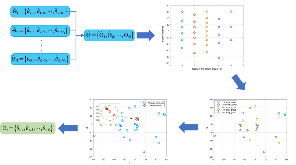
Figure 2: Cluster-based search method

Due to the fact that true angles of all group arrays will be close to each other, the extraction of true angles could be transferred into a cluster problem.

As shown in Fig. 2, all angles of all group arrays are obtained firstly. Then, convert the one-dimensional information $\theta$ into a two-dimensional scattered point diagram by $|\theta|e^{j\theta}$

$$I(\theta)=\mathbb{R}\left[\theta|e^{j\theta}|\right]$$

$$Q(\theta)=\mathbb{I}\left[\theta|e^{j\theta}|\right]$$ (48)

Observing the two-dimensional , the $Q$ points corresponding to true angles are almost coincident and others are discrete. Thus, the density-based spatial clustering of applications with noise (DBSCAN) method is able to be adopted [16]. DBSCAN algorithm could be summarized as three steps: 1) select a point randomly 2)

However, in our work, only $Q$ nearest point need to be distinguished. Thus, the least number of reachable points can be set as $Q$.

IV Theoretical Analysis

In this section, we analyze the theoretical performance of the proposed structure and the computational complexity of proposed methods.

IV-A Performance Accuracy

CRLB is a low bound of the error variance for an unbiased estimator. Thus, we derive the closed-form expression of the CRLB corresponding to the proposed HCMD structure. Furthermore, we adopt it as the benchmark of proposed structure.

Theorem 3: The lower bound of variance for unbiased DOA estimation method with the HCMD structure plotted in the Fig. 1 is given by

$$\sigma_{\theta_{0}}^{2}\geq\frac{1}{N}\mathbf{FIM}^{-1}$$ (49)

where

$$\mathbf{FIM}=\sum_{q=1}^{Q}\mathbf{FIM}_{q}$$ (50)

Proof: See Appendix B.

V Simulation Results

In this section, we present simulation results to assess the performance of proposed DOA estimator and the corresponding CRLB as a performance benchmark. Assuming a source impinge on the array and $M=496$, $Q=3$, $N=100$, $K_{1}=K_{2}=K_{3}=16$. In our simulation, all results are averaged over 2000 Monte Carlo realizations and root-mean-squared error (RMSE) is employed to indicate the performance, which is given by

$$RMSE=\left(\frac{1}{N_{simu}}\sum_{n_{simu}}^{N_{simu}}(\hat{\theta}_{n_{simu}}-\theta_{0})^{2}\right)^{\frac{1}{2}}$$ (51)

where $N_{simu}$ is the number of Monte Carlo realizations.

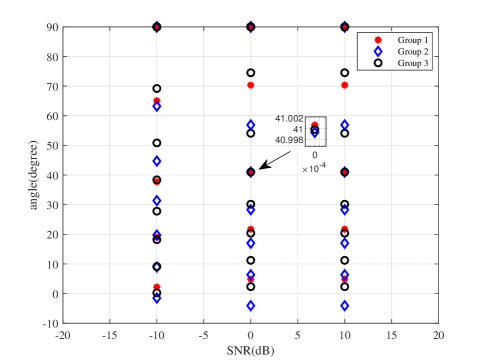
Figure 3: Angle of feasible solution set versus SNR of the proposed method

Fig. 3 plots the angle of feasible solution set for each group versus SNR of the proposed method for $M_{1}=7$, $M_{2}=11$ and $M_{3}=13$. From Fig. 3, it can be seen that there are $Q$ points in the candidate solution set generated by the $Q$ groups that are closest to each other, and these points are considered as $Q$ true solutions.

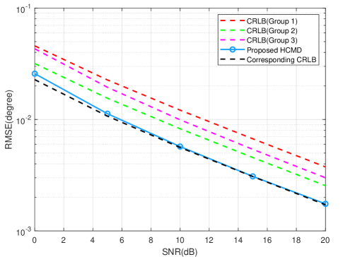
Figure 4: RMSE versus SNR of the proposed method

To further validate the conclusion of Fig. 3, Fig. 4 plots the root mean squared error (RMSE) versus SNR of the proposed DOA estimators HCMD for $M_{1}=7$, $M_{2}=11$ and $M_{3}=13$, where the corresponding CRLB and CRLB are used as performance benchmarks. From Fig. 4, it is seen that the proposed HCMD method can accurately find the true solutions in $Q$ groups and achieve the corresponding CRLB.

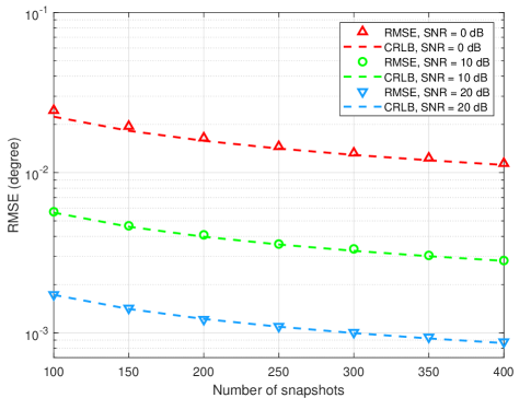
Figure 5: RMSE versus number of snapshots for the proposed method

VI Conclusions

In this paper, a high-performance DOA estimator HCMD is developed based on the heterogeneous hybrid MIMO receive structure. As the number of antennas tends to large-scale, the HCMD method can rapidly eliminate phase ambiguity and achieve excellent estimation performance. In particular, the proposed heterogeneous hybrid MIMO receive array not only significantly reduces circuit costs, but also provides a novel way to rapidly eliminate phase ambiguity through internal structure. This strikes an excellent balance between accuracy and complexity, making DOA estimation for massive MIMO receivers feasible for future practical applications such as UAV and web3.0.

APPENDIX A: Proof of Theorem 2

According to (III-A), we can define the Lagrangian function, $L(w_{q},\lambda^{\prime})$, as

$$L(w_{q},\lambda^{\prime})=\sum_{q=1}^{Q}w_{q}^{2}CRLB_{q}-\lambda^{\prime}\left(\sum_{q=1}^{Q}w_{q}-1\right)$$ (52)

where $\lambda^{\prime}$ is the Lagrange multiplier. The corresponding partial derivatives are given by

$$\frac{\partial L(w_{q},\lambda^{\prime})}{\partial w_{q}}=2w_{q}CRLB_{q}-\lambda^{\prime}$$ (53)

$$\frac{\partial L(w_{q},\lambda^{\prime})}{\partial\lambda^{\prime}}=-\sum_{q=1}^{Q}w_{q}+1$$ (54)

Since (52) is a convex quadratic function of $w_{q}$, we can set

$$\begin{split}\left\{\begin{array}[]{ll}\frac{\partial L(w_{q},\lambda^{\prime})}{\partial w_{q}}=0\\ \frac{\partial L(w_{q},\lambda^{\prime})}{\partial\lambda^{\prime}}=0\end{array}\right.\end{split}$$ (55)

which yields

$$w_{q}=\frac{CRLB_{q}^{-1}}{\sum_{q=1}^{Q}\left(CRLB_{q}\right)^{-1}}$$ (56)

Therefore, the proof of Theorem 2 is completed.

APPENDIX B: FIM for the HCMD structure

In this section, we derive the FIM for the HCMD structure. The FIM can be expressed as

$$\mathbf{FIM}_{\mathbf{y}}=\mathbf{Tr}\left\{\mathbf{R}_{\mathbf{y}}^{-1}\frac{\partial\mathbf{R}_{\mathbf{y}}}{\partial\theta}\mathbf{R}_{\mathbf{y}}^{-1}\frac{\partial\mathbf{R}_{\mathbf{y}}}{\partial\theta}\right\}$$ (57)

where

$$\mathbf{y}=[\mathbf{y}_{1},\mathbf{y}_{2},\cdots,\mathbf{y}_{Q}]^{T}=\mathbf{B}_{A}^{H}\mathbf{a}s+\mathbf{w}$$ (58)

where

$$\mathbf{B}_{A}=\left[\begin{array}[]{cccc}\mathbf{B}_{A,1}&\mathbf{0}&\cdots&\mathbf{0}\\ \mathbf{0}&\mathbf{B}_{A,2}&\cdots&\mathbf{0}\\ \vdots&\vdots&\ddots&\vdots\\ \mathbf{0}&\mathbf{0}&\cdots&\mathbf{B}_{A,Q}\end{array}\right]$$ (59)

$$\mathbf{a}=\left[\varphi_{1}\mathbf{a}_{1}^{T},\varphi_{2}\mathbf{a}_{2}^{T},\cdots,\varphi_{Q}\mathbf{a}_{Q}^{T}\right]^{T}$$ (60)

where

$$\varphi_{q}=\left\{\begin{array}[]{ll}1&,q=1\\ e^{j\frac{2\pi}{\lambda}d\sin\theta_{0}\sum_{q_{j}=1}^{q-1}N_{q_{j}}}&,q>1\end{array}\right.$$ (61)

$$\mathbf{R}_{\mathbf{y}}=\gamma\mathbf{B}_{A}^{H}\mathbf{a}\mathbf{a}^{H}\mathbf{B}_{A}+\mathbf{I}$$ (62)

Then, submitting (59)-(61) into (62), we can simplify the (62) as (75),

$$\mathbf{R}_{\mathbf{y}} =\gamma\left[\begin{array}[]{cccc}\mathbf{B}_{A,1}^{H}&\mathbf{0}&\cdots&\mathbf{0}\\ \mathbf{0}&\mathbf{B}_{A,2}^{H}&\cdots&\mathbf{0}\\ \vdots&\vdots&\ddots&\vdots\\ \mathbf{0}&\mathbf{0}&\cdots&\mathbf{B}_{A,Q}^{H}\end{array}\right]\left[\begin{array}[]{c}\varphi_{1}\mathbf{a}_{1}\\ \varphi_{2}\mathbf{a}_{2}\\ \vdots\\ \varphi_{Q}\mathbf{a}_{Q}\end{array}\right]\left[\varphi_{1}^{H}\mathbf{a}_{1}^{H},\varphi_{2}^{H}\mathbf{a}_{2}^{H},\cdots,\varphi_{Q}^{H}\mathbf{a}_{Q}^{H}\right]\left[\begin{array}[]{cccc}\mathbf{B}_{A,1}&\mathbf{0}&\cdots&\mathbf{0}\\ \mathbf{0}&\mathbf{B}_{A,2}&\cdots&\mathbf{0}\\ \vdots&\vdots&\ddots&\vdots\\ \mathbf{0}&\mathbf{0}&\cdots&\mathbf{B}_{A,Q}\end{array}\right]+\mathbf{I}$$ (75)

$$=\gamma\left[\begin{array}[]{cccc}\mathbf{B}_{A,1}^{H}\mathbf{a}_{1}\mathbf{a}_{1}^{H}\mathbf{B}_{A,1}&\mathbf{0}&\cdots&\mathbf{0}\\ \mathbf{0}&\mathbf{B}_{A,2}^{H}\mathbf{a}_{2}\mathbf{a}_{2}^{H}\mathbf{B}_{A,2}&\cdots&\mathbf{0}\\ \vdots&\vdots&\ddots&\vdots\\ \mathbf{0}&\mathbf{0}&\cdots&\mathbf{B}_{A,Q}^{H}\mathbf{a}_{Q}\mathbf{a}_{Q}^{H}\mathbf{B}_{A,Q}\end{array}\right]+\mathbf{I}=\left[\begin{array}[]{cccc}\mathbf{R}_{\mathbf{y}_{1}}&\mathbf{0}&\cdots&\mathbf{0}\\ \mathbf{0}&\mathbf{R}_{\mathbf{y}_{2}}&\cdots&\mathbf{0}\\ \vdots&\vdots&\ddots&\vdots\\ \mathbf{0}&\mathbf{0}&\cdots&\mathbf{R}_{\mathbf{y}_{Q}}\end{array}\right]$$ (84)

where

$$\mathbf{R}_{\mathbf{y}_{q}}=\gamma\mathbf{B}_{A,q}^{H}\mathbf{a}_{q}\mathbf{a}_{q}^{H}\mathbf{B}_{A,q}+\mathbf{I}$$ (85)

Thus, the FIM can be given by

$$\mathbf{FIM}_{\mathbf{y}} =\mathbf{Tr}\left\{\left[\begin{array}[]{cccc}\mathbf{R}_{\mathbf{y}_{1}}^{-1}\frac{\partial\mathbf{R}_{\mathbf{y}_{1}}}{\partial\theta}\mathbf{R}_{\mathbf{y}_{1}}^{-1}\frac{\partial\mathbf{R}_{\mathbf{y}_{1}}}{\partial\theta}&\mathbf{0}&\cdots&\mathbf{0}\\ \mathbf{0}&\mathbf{R}_{\mathbf{y}_{2}}^{-1}\frac{\partial\mathbf{R}_{\mathbf{y}_{2}}}{\partial\theta}\mathbf{R}_{\mathbf{y}_{2}}^{-1}\frac{\partial\mathbf{R}_{\mathbf{y}_{2}}}{\partial\theta}&\cdots&\mathbf{0}\\ \vdots&\vdots&\ddots&\vdots\\ \mathbf{0}&\mathbf{0}&\cdots&\mathbf{R}_{\mathbf{y}_{Q}}^{-1}\frac{\partial\mathbf{R}_{\mathbf{y}_{Q}}}{\partial\theta}\mathbf{R}_{\mathbf{y}_{Q}}^{-1}\frac{\partial\mathbf{R}_{\mathbf{y}_{Q}}}{\partial\theta}\end{array}\right]\right\}=\sum_{q=1}^{Q}\mathbf{FIM}_{q}$$ (90)

$$CRLB =\frac{1}{N}\mathbf{FIM}_{\mathbf{y}}^{-1}$$

$$=\frac{1}{N}\left(\sum_{q=1}^{Q}\mathbf{FIM}_{q}\right)^{-1}$$

Thus, the closed-form expression of the FIM for the HCMD structure is derived

References

- [1] R. M. B. Seyed A. Reza Zekavat, Handbook of Position Location: Theory, Practice, and Advances. Wiley-IEEE Press, NJ 08854, USA, 2019.
- [2] B. Shi, Y. Li, G. Wu, R. Chen, S. Yan, and F. Shu, “Low-Complexity Three-Dimensional AOA-Cross Geometric Center Localization Methods via Multi-UAV Network,” Drones, vol. 7, no. 5, 2023.
- [3] Y. Wang and K. C. Ho, “An asymptotically efficient estimator in closed-form for 3-D AOA localization using a sensor network,” IEEE Trans. Wireless Commun., vol. 14, no. 12, pp. 6524–6535, 2015.
- [4] ——, “Unified near-field and far-field localization for AOA and hybrid AOA-TDOA positionings,” IEEE Trans. Wireless Commun., vol. 17, no. 2, pp. 1242–1254, 2018.
- [5] X. Cheng, F. Shu, Y. Li, Z. Zhuang, D. Wu, and J. Wang, “Optimal Measurement of Drone Swarm in RSS-Based Passive Localization With Region Constraints,” IEEE Open Journal of Vehicular Technology, vol. 4, pp. 1–11, 2023.
- [6] T. E. Tuncer and B. Friedlander, Classical and Modern Direction-of-Arrival Estimation. Burlington, MA 01803, USA, 2009.
- [7] X. Huang and B. Liao, “One-bit music,” IEEE Signal Processing Letters, vol. 26, no. 7, pp. 961–965, 2019.
- [8] Z. Zheng, N. Guo, and W.-Q. Wang, “Angle estimation for bistatic mimo radar using one-bit sampling via atomic norm minimization,” IEEE Transactions on Aerospace and Electronic Systems, vol. 58, no. 6, pp. 5815–5822, 2022.
- [9] C.-J. Wang, C.-K. Wen, S. Jin, and S.-H. Tsai, “Gridless channel estimation for mixed one-bit antenna array systems,” IEEE Transactions on Wireless Communications, vol. 17, no. 12, pp. 8485–8501, 2018.
- [10] B. Shi, N. Chen, X. Zhu, Y. Qian, Y. Zhang, F. Shu, and J. Wang, “Impact of Low-Resolution ADC on DOA Estimation Performance for Massive MIMO Receive Array,” IEEE Syst J, pp. 1–4, 2022.
- [11] B. Shi, Q. Zhang, R. Dong, Q. Jie, S. Yan, F. Shu, and J. Wang, “DOA Estimation for Hybrid Massive MIMO Systems Using Mixed-ADCs: Performance Loss and Energy Efficiency,” IEEE Open Journal of the Communications Society, vol. 4, pp. 1383–1395, 2023.
- [12] F. Shu, Y. Qin, T. Liu, L. Gui, Y. Zhang, J. Li, and Z. Han, “Low-Complexity and High-Resolution DOA Estimation for Hybrid Analog and Digital Massive MIMO Receive Array,” IEEE Trans. Commun, vol. 66, no. 6, pp. 2487–2501, 2018.
- [13] B. Shi, X. Jiang, N. Chen, Y. Teng, J. Lu, F. Shu, J. Zou, J. Li, and J. Wang, “Fast Ambiguous DOA Elimination Method of DOA Measurement for Hybrid Massive MIMO Receiver,” Sci. China Inf. Sci., vol. 65, no. 5, 2022.
- [14] D. Hu, Y. Zhang, L. He, and J. Wu, “Low-Complexity Deep-Learning-Based DOA Estimation for Hybrid Massive MIMO Systems With Uniform Circular Arrays,” IEEE Wireless Commun. Lett., vol. 9, no. 1, pp. 83–86, 2020.
- [15] B. Friedlander, “The root-MUSIC algorithm for direction finding with interpolated arrays,” Signal Processing, 1993.
- [16] M. Ester, H.-P. Kriegel, J. Sander, X. Xu et al., “A density-based algorithm for discovering clusters in large spatial databases with noise,” in kdd, vol. 96, no. 34, 1996, pp. 226–231.