Unbiased Decisions Reduce Regret: Adversarial Domain Adaptation for the Bank Loan Problem

Abstract

In many real world settings binary classification decisions are made based on limited data in near real-time, e.g. when assessing a loan application. We focus on a class of these problems that share a common feature: the true label is only observed when a data point is assigned a positive label by the principal, e.g. we only find out whether an applicant defaults if we accepted their loan application. As a consequence, the false rejections become self-reinforcing and cause the labelled training set, that is being continuously updated by the model decisions, to accumulate bias. Prior work mitigates this effect by injecting optimism into the model, however this comes at the cost of increased false acceptance rate. We introduce adversarial optimism (AdOpt) to directly address bias in the training set using adversarial domain adaptation. The goal of AdOpt is to learn an unbiased but informative representation of past data, by reducing the distributional shift between the set of accepted data points and all data points seen thus far. AdOpt significantly exceeds state-of-the-art performance on a set of challenging benchmark problems. Our experiments also provide initial evidence that the introduction of adversarial domain adaptation improves fairness in this setting.

In a variety of online decision making problems, principals have to make an acceptance or rejection decision for a given instance based on observing data points in an online fashion. Across a broad range of these, the true label is only revealed for those data points which the principal accepted, creating a biased labelled dataset.

In this work we concentrate on addressing this issue for the specific class of binary classification tasks, also known as the “Bank Loan Problem”(BLP), motivated by the characteristic example of a lender deciding on outcomes of loan applications. The lender’s objective is to maximize profit, i.e. accept as many credible applicants as possible, while denying those who would ultimately default. The caveat is that the lender doesn’t learn whether rejected applicants would have actually repaid the loan. Hence a decision policy that relies solely on the past experience lacks the opportunity to correct for erroneous rejection decisions. These “false rejects” are self-reinforcing since the correct label is never revealed for rejected candidates.

As time progresses, the growing pool of accepted applicants (the models training set), created by the models decisions, forms an increasingly biased dataset, whose distribution is different from that of the general applicant population. This distributional shift affects the accuracy of the predictions of a model trained on the set of accepted points for any future applicants.

We propose and evaluate a novel approach to the BLP that is motivated by methods from the domain of learning in the presence of distributional shift. Specifically, we utilize adversarial domain adaptation to learn a de-biased representation of the training data that minimizes this distributional difference, while preserving the informative features. Although very natural in this setting, this is to our knowledge the first attempt to utilise adversarial domain adaptation to tackle bias in the online context.

Our experiments show that the adversarially de-biased classifier trained on the above “domain-agnostic” representation of the data achieves increased recall on the new queries, and thus mitigates the issue of self-reinforcing false rejections. However, on its own the adversarially de-biased classifier suffers from a fundamental flaw: It needs to trade-off between truly informative features and reducing bias. Clearly, both objectives cannot be perfectly accomplished at the same time, which causes this method to perform poorly on some datasets. To overcome this issue we propose adversarial optimism method (AdOpt), which combines the de-biased classification approach with the recently proposed Pseudo-Label Optimism(PLOT) (Pacchiano et al. 2021). PLOT is a strategy for injecting optimism into a model by adding each incoming query to the dataset with a positive pseudo-label and re-training an optimistic classifier on the resulting dataset. However when this strategy is applied indiscriminately to all incoming queries it suffers from greatly increased false acceptance rate. AdOpt proposes an alternative to this approach by first filtering the incoming queries using the adversarially de-biased classifier to assess the probability of a query being a true positive. In other words, AdOpt proposes a data driven strategy for selecting pseudo-label candidates.

Since the de-biased classifier is able to choose positives with better accuracy, its utilisation allows AdOpt to converge after seeing a smaller number of candidates and with fewer misclassified queries, as evidenced by its lower regret in our experiments. AdOpt consistently outperforms other established approaches from the literature, namely PLOT, “greedy”, $\epsilon$-greedy (with a decaying schedule) and NeuralUCB (Zhou, Li, and Gu 2020) algorithms (see Figure  1). Conducting high number of experiments across several sampling methods allows us to confirm the statistical significance of our results with high accuracy (Figures  1,  5).

The term “de-biased classifier” in our context means a classifier that is trained on a representation of the data that diminishes differences between the accepted applicants and general population, hence a priori de-biasing in our sense doesn’t necessarily imply increased “fairness” e.g. towards applicants with protected characteristics. However we conduct some initial experiments to clarify whether that is the case. As Figure 2 illustrates, the adversarially de-biased classifier when used on its own in the BLP setup comes closer than the established approaches to satisfying the equality of odds definition of fairness. As a result AdOpt that incorporates adversarial de-biasing also performs better on this measure compared to PLOT. Remarkably, this increase in fairness is not due to explicitly controlling for bias towards protected characteristics, which usually comes at a trade-off with classification accuracy. To our knowledge our work is the first to evaluate fairness in the context of BLP. Our results indicate that incorporating adversarial de-biasing has potential to increase fairness, and proposes a potentially fruitful and socially relevant new direction for investigation.

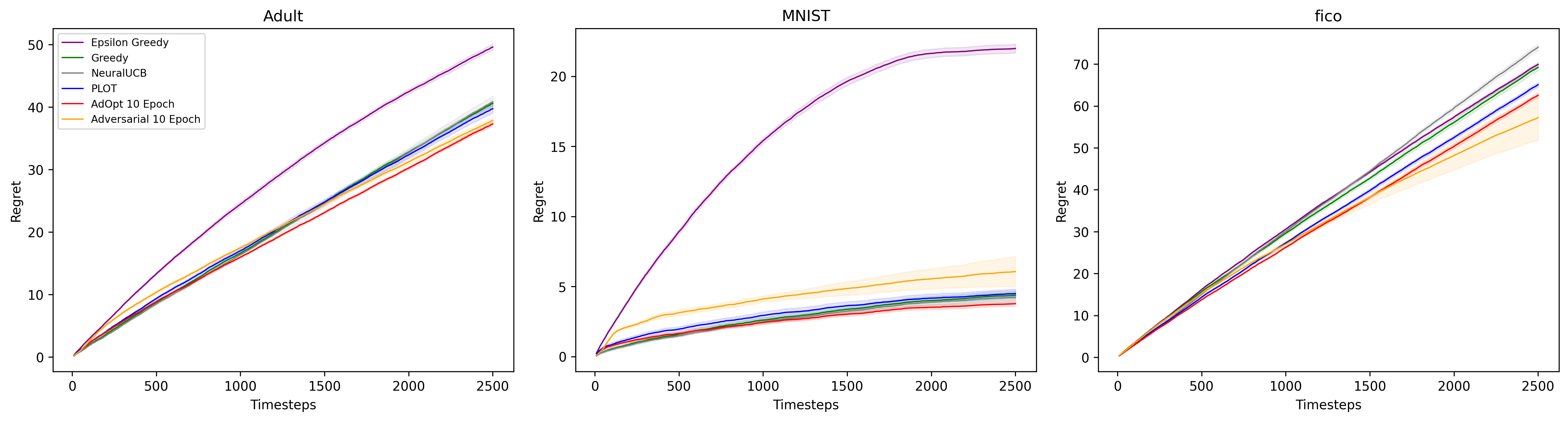
Figure 1: Cumulative regret of AdOpt vs. PLOT, NeuralUCB, Greedy and Epsilon-greedy methods on the UCB dataset Census Income (“Adult”) as well as MNIST and FICO challenge dataset(“FICO”). We also evaluate the adversarially de-biased classifier on its own as an ablation (“Adversarial”). The adversarial component is trained for 10 epoch at each batch. Cumulative regret is reported as a function of timestep (batch) and expressed in multiples of batch size, i.e. one unit of regret on the graph signifies 32 misclassifications. The shaded region represents one standard deviation from the mean, computed across 25 experiments, 5 runs over 5 different sampling methods. We find that AdOpt outperforms the previous SOTA methods by a significant margin while displaying stable performance for all datasets and seeds evidenced by its narrow STD interval.

Related work

Contextual bandits and function approximation

The Bank Loan problem (BLP) is a specific instance of a contextual bandit problem with two possible actions and a reward function that is 1 if the accepted applicant returns the loan, -1 if he doesn’t and 0 if the lender decides to reject the applicant. There exist a multitude of methods for this setting ranging from adversarial bandit approaches such as EXP4 (Auer et al. 2002) to methods that rely on simple parametric assumptions on the data (for example linear responses) such as OFUL (Abbasi-Yadkori, Pál, and Szepesvári 2011) or GLM (Filippi et al. 2010). These methods’ applicability to the BLP depends on the data satisfying restrictive parametric assumptions. Specifically, these methods are not compatible with the use of deep neural network (DNN) function approximators.

Neural solutions to the bank loan problem

More recently, deep neural networks have been successfully applied to this class of problems, with several proposed strategies (Riquelme, Tucker, and Snoek 2018; Zhou, Li, and Gu 2020; Xu et al. 2020). For example, in (Riquelme, Tucker, and Snoek 2018) the authors conduct an extensive empirical evaluation of existing bandit algorithms on public datasets. A more recent line of work has focused on devising ways to add optimism to the predictions of neural network models. Methods such as Neural UCB and Shallow Neural UCB (Zhou, Li, and Gu 2020; Xu et al. 2020) are designed to add an optimistic bonus to the model predictions that is a function of the representation layers of the model. Their theoretical analysis is inspired by insights gained from Neural Tangent Kernel theory. Other recent works in the contextual bandit literature such as (Foster and Rakhlin 2020) have started to pose the question of how to extend theoretically valid guarantees into the function approximation scenario, so far with limited success (Sen et al. 2021).

The PLOT method from (Pacchiano et al. 2021) provides a simple and computationally efficient way to introduce optimism which can be used in combination with deep neural networks. This optimism translates self-fulfilling false rejects into self-correcting false accepts by the way of introducing pseudo-labelled queries to the model training set. However, this approach suffers from increased false acceptance rate in particular early on in the learning process. Therefore while the above approach has the benefit of theoretical performance guarantees, to obtain SOTA empirical results in (Pacchiano et al. 2021) the authors mitigate this problem by assigning pseudo-labels with fixed (small) probability $\epsilon$. However such one-size-fits-all approach doesn’t take into account the intrinsic properties of the dataset or a specific query which hinders performance when comprehensively evaluated across several sampling methods. In the present work evaluation across several seeds on the MNIST and Credit datasets shows that on average PLOT ties with NeuralUCB, whereas AdOpt outperforms both by a significant margin, as evidenced by the relative t-values we report in Table 2.

Selective labels

The bank loan problem is also known as the“selective labels” problem (Lakkaraju et al. 2017), but the majority of the literature in this area so far focuses on the offline setup. The recent paper (Wei 2021) considers online scenario, but in contrast with our setting their online mechanism requires the data distribution to be stationary. Additionally although the authors mention their methods can be extended to the setting of NNs, their experimental evaluation is conducted mainly over linear models.

Reject inference

This line of methods attempts to correct bias in credit scoring by modelling the missing outcomes of the rejected applications. While statistical and machine learning methods are most commonly used, more recently deep learning methods have also been applied (Mancisidor et al. 2020). However, like in the majority of selective labels literature, the online scenario has not been considered.

Fairness

Fairness is a central concern in algorithmic decision-making and existing literature offers numerous approaches and perspectives. Fairness in the contextual bandits setting is explored in (Joseph et al. 2016; Schumann et al. 2019). Domain adaptation techniques for censoring of protected features were proposed and evaluated by (Edwards and Storkey 2016; Zhang, Lemoine, and Mitchell 2018) among others and (Coston et al. 2019; Singh et al. 2021) address fairness in the context of distributional shift. The above works do not consider the online setting, or more specifically the BLP. In the setup of “selective labels” (Kilbertus et al. 2020) considers learning under fairness constraints under assumption of stationary data distribution (not required by our method) and (Coston, Rambachan, and Chouldechova 2021) proposes a method for selecting fair models from existing ones.

Repeated Loss Minimization

Previous works (Hardt et al. 2016; Hashimoto et al. 2018) have studied the problem of repeated classification settings where the underlying distribution is influenced by the model itself. The works (Perdomo et al. 2020; Miller, Perdomo, and Zrnic 2021) extend this idea to introduce the problem domains of strategic classification and performative prediction. Unlike in the above setting, in our case only the labelled training set is affected by the model, leading to a distributional shift between this set and the set of points presented to the model. This shift is precisely the reason for suitability of domain adaptation to our setting.

Background

The bank loan problem

We are focusing on the class of sequential learning tasks, where at every timestep $t$, the learner is presented with a query $\mathbf{x}_{t}\in\mathbb{R}^{d}$ and needs to predict its binary label $y_{t}\in\{0,1\}$. Acceptance of the query carries an unknown reward of $2y_{t}-1$ and rejection a fixed reward of $0$. Using the bank loan analogy, the lender receives a unit gain for accepting a customer who repays his loan, experiences a unit loss for accepting a customer who defaults and receives nothing if they reject an application. The learners objective is to maximize their reward, which is equivalent to maximizing the number of correct decisions made during training  (Kilbertus et al. 2020).

We assume that the distribution of the labels is given by a probability function $\rho_{\theta_{\star}}$:

$$y(\mathbf{x_{t}})=\begin{cases}1&\text{with probability }\rho_{\theta_{\star}}(\mathbf{x}_{t})\\ 0&\text{o.w.}\end{cases}$$ (1)

where $\rho_{\bm{\theta}_{\star}}:\mathbb{R}^{d}\rightarrow\mathbb{R}$ is a function parameterized by $\bm{\theta}_{\star}\in\Theta$. Note that the distribution of the query points $\mathcal{P}(\mathbf{x})$ may be different for different $t$’s: e.g. the bank may extend it’s loan provision at a certain time point $t_{0}$ and start targeting a different applicant demographic.

We assume that the learners decision at time $t$ is parameterized by $\bm{\theta}_{t}$ and is given by the rule:

$$\text{If }\rho_{\bm{\theta}_{t}}(\bm{x}_{t})\geq\frac{1}{2}\text{ accept }$$

A common measure of the learners performance is regret:

$$\mathcal{R}(t)=\sum_{\ell=1}^{t}\max(0,2\rho_{\bm{\theta}_{\star}}(\mathbf{x}_{\ell})-1)-a(\mathbf{x}_{\ell})(2\rho_{\bm{\theta}_{\star}}(\mathbf{x}_{\ell})-1)$$

where we denote by $a(\mathbf{x}_{\ell})\in\{0,1\}$ the indicator of whether the learner has decided to accept (1) or reject (0) the data point $\mathbf{x}_{\ell}$.

Minimizing regret is a standard objective in the online learning and bandits literature (see (Lattimore and Szepesvári 2020)).

Using the set of accepted data points, i.e. the greedy approach, $\rho_{\bm{\theta}_{t}}$ can be obtained by minimising binary cross entropy loss:

$$\mathcal{L}(\bm{\theta}|\mathcal{A}_{t}) =\sum_{\mathbf{x}\in\mathcal{A}_{t}}-y(\mathbf{x})\log\left(\rho_{\bm{\theta}}(\bm{x})\right)$$ (2)

$$-(1-y(\mathbf{x}))\log\left(1-\rho_{\bm{\theta}}(\mathbf{x})\right)$$

where $\mathcal{A}_{t}=\{\mathbf{x}_{\ell}|a_{\ell}=1\text{ and }\ell\leq t-1\}$ denotes the dataset of accepted points up to the time $t-1$. In what follows we call such $\rho_{\bm{\theta}_{t}}$ the biased model.

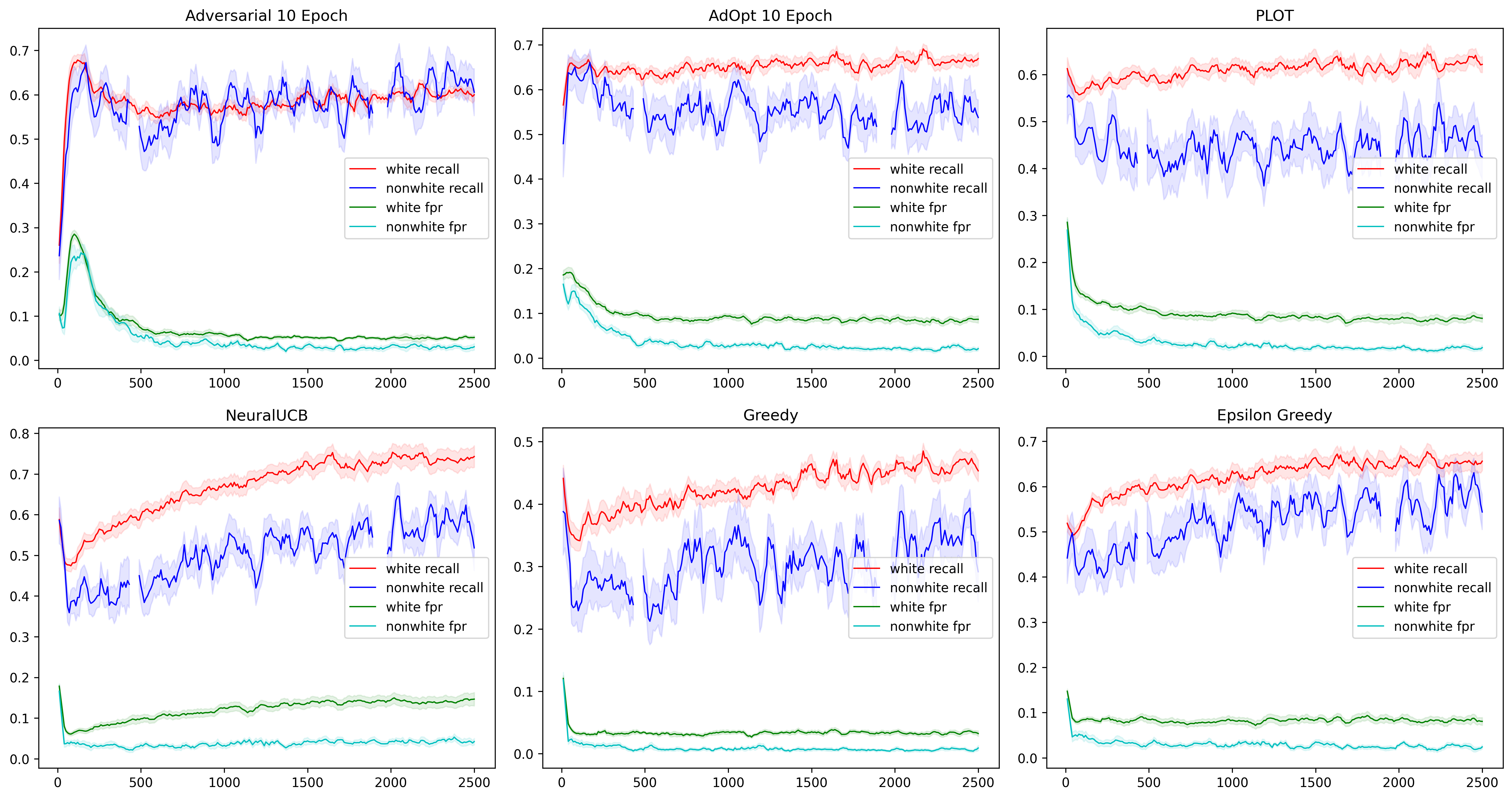
Figure 2: The recall and false positives ratio (fpr) values per batch for “White” and “Other” subgroups of the Census Income(“Adult”) dataset. The adversarially de-biased classifier is the only one among evaluated methods that shows similar values of recall (tpr) and fpr for these groups, thus coming close to satisfying the equality of odds definition of fairness.

Adversarial domain adaptation

Domain adaptation studies strategies for learning in the presence of distributional shift between the labelled data used for training and the unlabelled data domain containing test samples. Adversarial domain adaptation, first proposed in (Ganin et al. 2016), is based on the theory of distance between domains introduced in (Ben-David et al. 2006, 2010) and the GAN approach of (Goodfellow et al. 2014). The main idea of this method is constructing a representation of the data that is both discriminative for the given classification task and domain invariant. Further work in adversarial domain adaptation has generalised the method to different adversarial loss functions and generative tasks, e.g. (Liu and Tuzel 2016; Tzeng et al. 2017; Zhang, Lemoine, and Mitchell 2018), and successfully applied it to a wide array of challenges, e.g. (Edwards and Storkey 2016; Wang et al. 2019). Our approach in the present work is similar to the DANN algorithm of (Ganin et al. 2016), that we found to give stable results for the duration of the training.

		Recall		Precision		Predicted Positive
	True Pos.	biased	de-biased	biased	de-biased	biased	de-biased	de-biased $\mathcal{S}$
Mean	0.24	0.59	0.83	0.78	0.31	0.18	0.66	0.69
STD	0.07	0.2	0.16	0.19	0.12	0.07	0.11	0.11

Table 1: Mean and STD values for performance metrics of biased (greedy) and adversarially de-biased classifiers on the Census Income (“Adult”) dataset. We find that adversarial de-biasing trades off precision and recall. All columns except the last contain metrics for the incoming batch, or “Target” $\mathcal{T}$. The last three columns contain the proportion of predicted positives for the incoming batch and the “Source” $\mathcal{S}$ set of accepted applicants to empirically validate that equation (4) holds.

Given a labelled source dataset $\mathcal{S}\subset\mathbb{R}^{d}$ and a target dataset $\mathcal{T}\subset\mathbb{R}^{d}$ whose labels we need to predict, the adversarial domain adaptation approach is to simultaneously train a generator $G_{\theta}:\mathbb{R}^{d}\rightarrow\mathbb{R}^{d^{\prime}}$ that encodes the data, a classifier $C_{\psi}:\mathbb{R}^{d^{\prime}}\rightarrow\{0,1\}$, and a discriminator $D_{\phi}:\mathbb{R}^{d^{\prime}}\rightarrow\{0,1\}$ that discriminates between the encodings of samples from $\mathcal{S}$ and $\mathcal{T}$, so that $C_{\psi}(G_{\theta}(\cdot))$ has a high classification accuracy on $\mathcal{S}$, and $G_{\theta}$ is trained adversarially with $D_{\phi}$ to minimise the possibility of distinguishing between samples from $G_{\theta}(\mathcal{S})$ and $G_{\theta}(\mathcal{T})$. Following (Zhang, Lemoine, and Mitchell 2018) we will refer to the representation of the data by $G_{\theta}$ as “de-biased” and to $C_{\psi}$ as the “de-biased classifier” - “de-biased” in our context refers to a representation that doesn’t distinguish between test and train domains.

The training of generator, classifier, and discriminator can be summarised by the training objective $\min_{\theta}\min_{\psi}\max_{\phi}L_{\theta,\psi,\phi}$,

$$L_{\theta,\psi,\phi} :=\mathop{\mathbb{E}}_{\mathbf{x}\in\mathcal{T}}\log(D_{\phi}(G_{\theta}(\mathbf{x}))$$ (3)

$$+\mathop{\mathbb{E}}_{\mathbf{x}\in\mathcal{S}}\log(1-D_{\phi}(G_{\theta}(\mathbf{x})))$$

$$+L^{C}_{x\in\mathcal{S}}(C_{\psi}(G_{\theta}(\mathbf{x})),y(\mathbf{x})),$$

where $L^{C}$ is the binary cross entropy loss and $y:\mathcal{S}\rightarrow\{0,1\}$ provides the labels.

Adversarial domain adaptation approach to the Bank Loan Problem

Adversarial de-biasing in the BLP context

Let us recap the task at hand: in the BLP setting at time $t$ we possess a labelled set of previously accepted applicants $\mathcal{A}_{t}$ and we want to utilize this information to label a new applicant. The obstacle to overcome is that the distribution of the data points in the general applicant pool $\mathcal{A}$, is different from the distribution of data points in $\mathcal{A}_{t}$, that was influenced by the previous choices of the classifier. This will compromise the performance of a classifier trained on $\mathcal{A}_{t}$. We address this issue by using domain adaptation to find the de-biased representation $G_{\theta}$ of the data in $\mathcal{A}_{t}$ and train the de-biased classifier $C_{\phi}$ to predict a label for the candidate $\mathbf{x}$ sampled from $\mathcal{A}$.

We expect $C_{\phi}$ to give optimistic predictions for the labels of $\mathbf{x}\in\mathcal{A}$, in the following sense: as shown in (Edwards and Storkey 2016), adversarial domain adaptation produces a classifier and generator that converge to approximating the demographic parity property

$$P_{(C(G(\mathbf{x}))=1\mid\mathbf{x}\in\mathcal{S})}=P_{(C(G(\mathbf{x}))=1\mid\mathbf{x}\in\mathcal{T})}.$$ (4)

Equation (4) states that the percentage of positive predictions on the transformed labelled set $G_{\theta}(\mathcal{S})$ is the same as on $G_{\theta}(\mathcal{T})$. In the BLP setting, as the training progresses and the classifier becomes better at accepting the right candidates, the distribution of true positive labels in $\mathcal{A}_{t}$ diverges from that of the general population: for $t\gg 0$

$$P_{(y(\mathbf{x})=1|\mathbf{x}\in\mathcal{A}_{t})}>P_{(y(\mathbf{x})=1|\mathbf{x}\in\mathcal{A})}.$$ (5)

Note that the above is simply a consequence of the classifier being successful in its job and is independent of the accumulation of bias due to erroneous rejections. Since in the adversarial adaptation approach the classifier $C_{\psi}$ is trained to preserve the accuracy on the labelled set $\mathcal{A}_{t}$, $P(C_{\psi}(G_{\theta}(\mathbf{x}))=1)$ is going to be close to $P(y_{true}(\mathbf{x})=1|\mathbf{x}\in\mathcal{A}_{t})$ both when $\mathbf{x}\in\mathcal{A}_{t}$ and $\mathbf{x}\in\mathcal{A}$. In the BLP setting, the adversarial training regime creates de-biased classifier that optimistically overpredicts positive labels for the incoming queries.

To verify empirically that our adversarial training regime in the context of BLP produces de-biased classifier with properties as above, we create a performance metrics log across the experiments comparing the performance of the de-biased classifier and the classifier trained on the original biased data. The mean and standard deviation for the de-biased classifier that is trained from scratch at each step are in Table 1. The last two columns empirically evaluate Equation (4).

For practical realisation to increase computational efficiency we consider the scenario, where at each time-step a learner receives a batch of data points $\mathcal{B}_{t}=\{\mathbf{x}_{t,1},\ldots,\mathbf{x}_{t,B}\}$. We obtain the pair consisting of de-biased classifier and the generator of de-biased data representation $(C,G)$ for the pair of source and target datasets $(\mathcal{A}_{t},\mathcal{B}_{t})$ by minimising the loss function (3) and use $C$ to obtain predictions for the labels of the data points in $\mathcal{B}_{t}$. We provide the details of the adversarial training algorithm in the Appendix.

As can be seen from Table 1, increased recall of the adversarially de-biased classifier comes at the expense of lower precision. This trade off can be regulated by the length of adversarial training. We empirically found that for minimizing regret best performance is achieved when training for small number of epochs at each step without resetting the weights of the adversarial triad. This approach also reduces the training duration.

Adversarial optimism

The adversarially de-biased classifier fails to reliably achieve the optimal results on all datasets (Figure 1), due to high false-positive rate and the inherent instability of the adversarial training, which causes the wide standard deviation on the regret plots. To mitigate for these drawbacks, we propose a new Adversarial Optimism (AdOpt) method, that combines the adversarially de-biased classifier with the pseudo-label optimism PLOT approach from (Pacchiano et al. 2021).

The PLOT approach is a simple yet efficient way to introduce optimism into a classification routine, which can be used with deep neural networks. The approach can be summarized as follows: to each new query $\mathbf{x}_{0}$ rejected by the “biased” classifier trained on all the accepted data so far it optimistically assigns a positive pseudo-label, retrains the model on the dataset that includes this data point with positive label and uses the resulting pseudo-label model to confirm or ignore the optimistic prediction.

Our proposed method, AdOpt uses two classifiers: the “biased” classifier and the adversarially de-biased one. Presented with a new data point AdOpt proceeds as follows:

• If a data point is accepted by the biased classifier, it is accepted and added to the dataset with the true label.

• If a data point is instead rejected by the biased classifier we use the de-biased classifier to decide whether to add it to the pseudo-label dataset to decide whether we should reconsider it for acceptance.

• We then apply the pseudo-label mechanism from PLOT, i.e. retraining on optimistic labels, on these candidates to decide final acceptance.

The last step of the algorithm evaluates the points that are recommended for acceptance by the de-biased classifier against the models prior knowledge by adding it to the original dataset with positive pseudo-labels and retraining an optimistic classifier to make a final decision. Incorporating prior model knowledge via PLOT mitigates against the high false acceptance rate, as well as the instability of adversarial training across batches and thus helps to further reduce regret incurred by our algorithm.

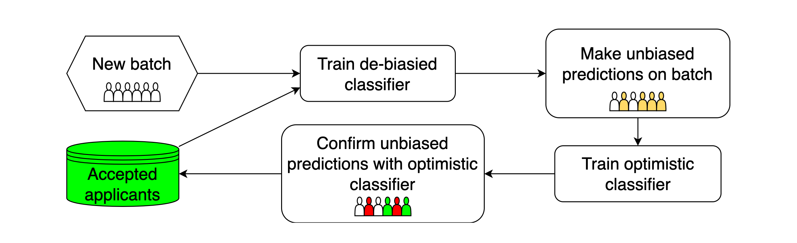
Figure 3: The AdOpt algorithm

Using the de-biased classifier for assigning pseudo-labels enables AdOpt to explore faster. The de-biased classifier possesses increased recall. While this comes at expense of lower precision, its acceptance suggestions are superior to randomly picking pseudo-label candidates as is done in (Pacchiano et al. 2021).

As before, in practice at every step we consider a batch of data points $\mathcal{B}_{t}$. During the very first time-step ($t=1$), the algorithm accepts all the points in $\mathcal{B}_{1}$. In subsequent time-steps we train a de-biased classifier adversarially for every timestep on the pair $(\mathcal{A}_{t},\mathcal{B}_{t})$. We identify a subset of the current batch $\mathcal{B}_{t}^{0}\subset\mathcal{B}_{t}$ composed of those points that are both currently being predicted as rejects by the biased model and have been selected as potential positives by the de-biased classifier. They comprise the pseudo-label batch of potential candidates for acceptance. We train the pseudo-label model on the combined dataset and accept those data points, whose labels were confirmed by the pseudo-label model predictions. The pseudo-label loss is given by adding a term to the loss function:

$$\mathcal{L}^{\mathcal{C}}(\bm{\theta}|\mathcal{A}_{t},\mathcal{B}_{t}) =\mathcal{L}(\bm{\theta}|\mathcal{A}_{t}\cup\{(\mathbf{x},1)\text{ for }\mathbf{x}\in\mathcal{B}_{t}\})$$ (6)

$$=\sum_{\mathbf{x}\in\mathcal{A}_{t}}-y\log\left(\rho_{\bm{\theta}}(\mathbf{x})\right)$$

$$-(1-y)\log(1-\rho_{\bm{\theta}}(\mathbf{x}))$$

$$-\underbrace{\sum_{\bm{x}\in\mathcal{B}_{t}^{0}}\log(\rho_{\bm{\theta}}(\mathbf{x}))}_{\text{pseudo-label loss}},$$

Algorithm 1 AdOpt

Initialize accepted dataset $\mathcal{A}_{1}=\emptyset$
For $t=1,\cdots,T$
1. Observe batch $\mathcal{B}_{t}=\{\mathbf{x}_{t}^{(j)}\}_{j=1}^{B}$.
2. Run adversarial domain adaptation algorithm with starting weights initialized from training $\mathcal{B}_{t-1}$ on $(\mathcal{A}_{t},\mathcal{B}_{t})$ to obtain generator and classifier pair $(G,C)$.
3. Train the biased model $\rho_{\bm{\theta}_{t}}$ by minimizing the loss $\mathcal{L}_{t}(\bm{\theta}|\mathcal{A}_{t})$.
4. Compute the pseudo-label filtered batch $\mathcal{B}_{t}^{0}=\{(\mathbf{x}_{t}^{(j)},1)\mid\rho_{\bm{\theta}_{t}}(\mathbf{x}_{t}^{(j)})<\frac{1}{2}\text{ and }C(G(x_{t}^{j}))=1\}$.
5. Train the pseudo-label model by minimizing the optimistic pseudo-label loss, $\mathcal{L}_{t}^{\mathcal{C}}(\bm{\theta}|\mathcal{A}_{t},\widetilde{\mathcal{B}}_{t})$
6. For $\mathbf{x}^{(j)}\in\mathcal{B}_{t}$ compute acceptance decision via $a^{(j)}_{t}=\begin{cases}1&\text{if }\rho_{\bm{\theta}^{C}_{t}}(\bm{x}_{t})\geq\frac{1}{2}\text{ or }\rho_{\bm{\theta}_{t}}(\bm{x}_{t})\geq\frac{1}{2}\\ 0&\text{o.w.}\end{cases}$
7. Update $\mathcal{A}_{t+1}\leftarrow\mathcal{A}_{t}\cup\{(\mathbf{x}^{(j)}_{t})\}_{j\in\{1,\cdots,B\}\text{ s.t. }a_{t}^{(j)}=1}$.

A notable feature of PLOT is that as the size of the dataset of accepted points grows, the predictions of the pseudo-label model differ less and less from the predictions of the biased model trained on the set of the accepted points. Ideologically once the dataset is sufficiently large and accurate information can be inferred about the true labels, the inclusion of $\mathcal{B}_{t}^{0}$ into the pseudo-label loss has vanishing effect on the model’s predictions. The latter has the beneficial effect of making false positive rate decrease with $t$. This balances the opposite trend in the predictions of the de-biased adversarial classifier, that tends to predicting more positives as the training progresses as a result of the Equations (5) and (4).

Fairness aspects

The datasets considered in the BLP context can explicitly or implicitly reveal sensitive information, such as e.g. gender or race. It is therefore natural to ask to what extent the methods in the BLP domain satisfy fairness criteria. While a comprehensive evaluation with respect to the multitude of definitions of fairness (Verma and Rubin 2018; Hertweck and Räz 2022) would be well beyond of the scope of our paper, both intuition and prior works (Edwards and Storkey 2016; Zhang, Lemoine, and Mitchell 2018) suggest that de-biased classifier should perform well for at least some of these metrics. To elaborate, consider for example the positively labelled (i.e. “persons with income greater than USD 50K”) subset of Census Income(“Adult”) dataset. We find that males and Whites are overrepresented compared to females and representatives of all other races respectively. It follows that in BLP setting the classifier will encounter significantly less positively labelled females and non-Whites than males and Whites, and the self-reinforcing false rejections phenomenon would make it prone to acquiring negative bias towards these groups. The above analysis shows that fairness investigation is warranted in this setting. Adversarial de-biasing should be able to partially mitigate this effect, because it uses a representation of the data which doesn’t distinguish between the accepted applicants and the applicants in the current batch. We verify this effect empirically in Figure 2: our experiments on the “Adult” dataset show that adversarially de-biased classifier comes close to satisfying the equality of odds definition of fairness: namely the true positive rate (TPR) or “recall” and the false positive rate (FPR) are close for the “Whites” and “Others” subgroups of the dataset. In the meanwhile the leading approaches to BLP show markedly different results for these subgroups. The intuition behind the equality of odds definition in the Bank Loan Problem language can be formulated as a requirement that

• Credible customers from both groups should be awarded similar opportunities.

• No unfair opportunity advantage should be given to those customers that are going to default for either group.

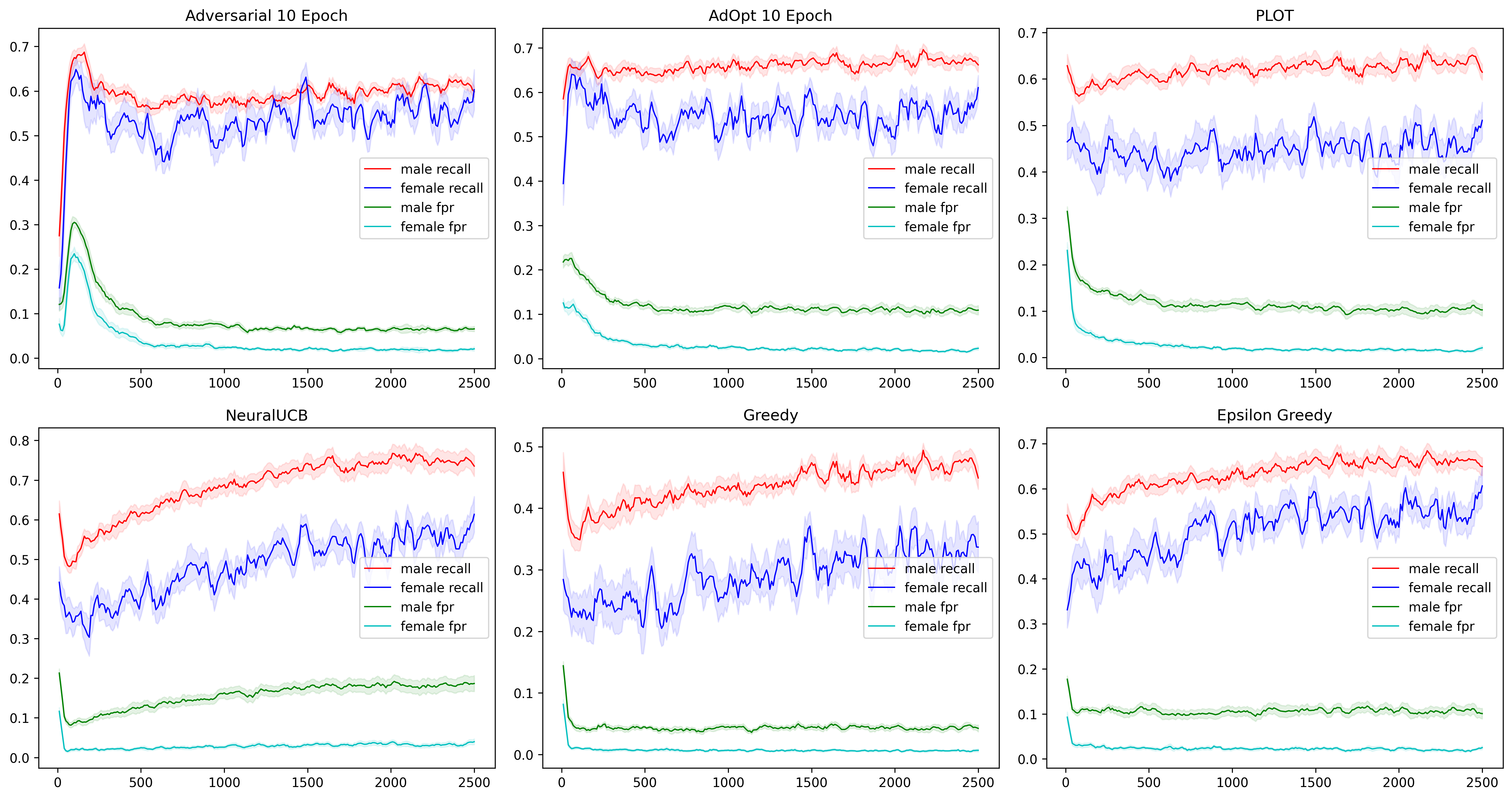
Figure 6: The recall and false positives ratio (fpr) values per batch for Females and Males subgroups of the “Census Income” dataset for the different methods evaluated in the paper. The adversarially de-biased classifier is the only one among evaluated methods that shows similar values of recall and FPR for these groups, thus coming close to satisfying the equality of odds definition of fairness.

The results for the female/male subgroups are similar and are presented in Figure 6. We note that incorporation of adversarially de-biased classifier in AdOpt improves its performance on this metric compared to PLOT.

We defer the more through investigation of fairness aspects to future work.

Experiments

Datasets and methods

To assess the performance of adversarially de-biased classifier and AdOpt, we consider several benchmark datasets: the UCI datasets Census Income(“Adult”) and Default of Credit Card Clients (Lichman et al. 2013), as well as the anonymized dataset of home equity line of credit (HELOC) (FICO. Explainable machine learning challenge ) and MNIST converted to the binary reward format of the BLP by defining the positive class to be images of the digit 5. “Adult” contains demographic information useful for fairness evaluation, and was used in in (Pacchiano et al. 2021) alongside MNIST, while FICO and “Credit” are publicly available real life datasets used for financial credibility evaluation. We train adversarially de-biased classifier for 10 epochs at each step.

We compare against four baseline methods: PLOT, NeuralUCB, Greedy (no exploration), and decayed $\epsilon$-greedy method. For $\epsilon$-greedy, we use a decayed schedule of (Kveton et al. 2019), dropping to 0.1% exploration by T=2500. We combine PLOT with $\epsilon$-greedy selection of pseudo-label candidates as in (Pacchiano et al. 2021).

Since sampling of batches presented during training as well as stochastic nature of optimisation has a significant effect on the final regret, to obtain the results in this paper we average the performance of each method across 5 different batch sampling methods and 5 separate runs of 2500 timesteps each, so altogether 25 experiments for each method. We note that this is different from the approach in  (Pacchiano et al. 2021) where only one specific way of sampling examples from the datasets was examined. This explains the difference in performance for PLOT on MNIST reported in this paper and in  (Pacchiano et al. 2021). We also note that, as opposed to  (Pacchiano et al. 2021), we report absolute values of regret at every step, rather than regret with respect to a baseline model, which allows us to achieve more transparent results. The high number of experiments allows us to conduct t-test and compute $0.95$ confidence intervals to evaluate statistical significance of reported results.

The number of training epochs for the adversarially de-biased classifier is a parameter that can be tuned to optimise the results for each dataset, however we chose to use fixed number of epochs for our comparisons in this paper, as it was already sufficient to demonstrate statistically significant advantage over the SOTA. The number of epochs also influences the runtime of the AdOpt algorithm. However we prioritise lower regret over faster runtime as for our purposes compute is cheap, while mistakes are costly. Further particulars on experiment details and hyperparameters can be found in appendix.

Main results

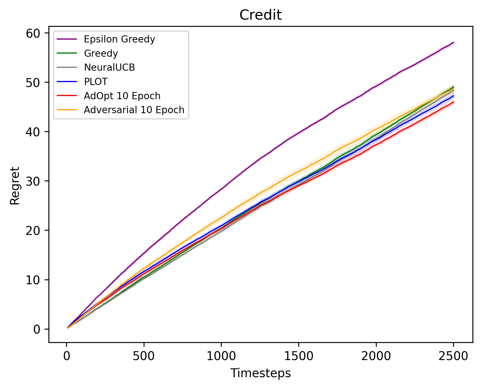
Figure 4: Cumulative regret of adversarially de-biased classifier (“Adversarial”) and AdOpt vs. PLOT, NeuralUCB, greedy and $\epsilon$-greedy methods on the UCI dataset Default of Credit Card Clients (“Credit”).

We report the following main results: We experimentally evaluate the performance of our proposed algorithm, AdOpt, that combines the adversarially de-biased classifier with the pseudo-labelling approach of (Pacchiano et al. 2021). We find that AdOpt significantly outperforms previously proposed methods. In Figures 1 and 4 we report cumulative regrets for each method.

To evaluate the significance of improvement of AdOpt over PLOT we compute paired t-values for each dataset in Table 2.

	Adult	FICO	MNIST	Credit
AdOpt	6.8798	6.7142	4.0966	4.1172

Table 2: Paired t-values of cumulative regret of AdOpt vs previous SOTA method PLOT at 2500 steps, where t-values of $>2$ indicate $<0.05$ chance of null-hypothesis.

In Figure 5 we display the corresponding $0.95$ CI for the difference between cumulative regrets of PLOT and AdOpt on “Adult” and MNIST datasets.

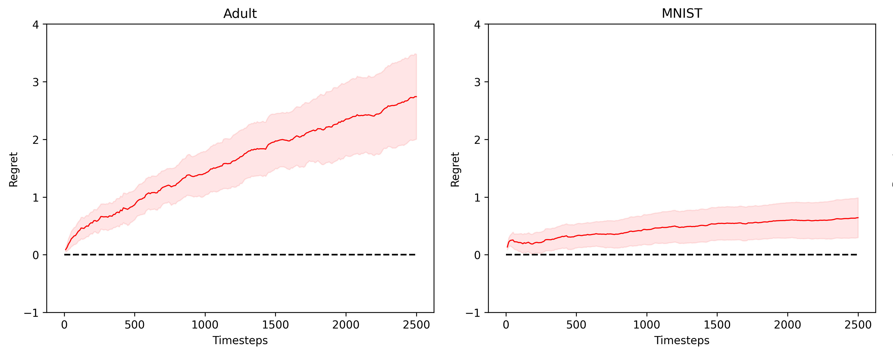
Figure 5: The difference of cumulative regrets for PLOT and AdOpt with $0.95$ confidence interval shaded on Census Income and MNIST datasets.

In Table 1, we compare the performance metrics for the adversarially de-biased classifier and the greedy classifier trained on the original biased data on the “Adult” dataset. The de-biased classifier achieves higher recall while maintaining predictive ability evidenced by its precision value.

We conduct experiments to evaluate fairness for the methods in the BLP domain. The results for the Census Income dataset are shown in Figures 2 and 6. Our experiments indicate that the adversarially de-biased classifier exhibits significantly less bias in its predictions for different subgroups within those categories, in particular displaying similar TPR and FPR values, and its incorporation within our proposed method, AdOpt, improves performance with respect to these metrics.

Conclusion

We apply adversarial domain adaptation to online learning to address the distributional shift accumulating due to past acceptance or rejection decisions. Our empirical evaluation indicates that the adversarially de-biased classifier has the potential to greatly reduce the risk of self-reinforcing rejection-loops, as well as increase fairness towards minority subgroups. We present AdOpt, a novel algorithm that incorporates adversarial domain adaptation and pseudo-label optimism and experimentally establishes a new SOTA across a variety of instances of the BLP with minimal hyperparameter tuning. Further directions include extensive exploration of other fairness aspects for online application of domain adaptation based methods, as well as generalisation of AdOpt to higher dimensional actions supporting applications to a variety of datasets and problem settings.

Appendix A Experiment details and hyperparameters

Our experiments use the optimal hyperparameters for each method reported in previous papers. NeuralUCB uses an alpha of $0.4$, and a discount factor of $0.9$. PLOT uses a two-layer, 40-node, multi-layer perceptron. AdOpt is trained using an encoded dimension of 100, as well as a hidden layer size of 100. Each experiment runs on a single GPU, and our results were collected by trivially distributing 25 experiments in parallel on 25 different GPU cores.

For the adversarial training, the generator, classifier, and discriminator are multi-layer perceptrons, where the dimension of the input, hidden layer(s), and output are $[\text{Data Dimension},100,100,100]$, $[100,100,1]$, and $[100,100,100,1]$ respectively. We used Adam optimizer, with $(\beta_{1},\beta_{2})=(0,0.99)$ and a learning rate of $0.0005$ for the discriminator and $0.0001$ for the generator and classifier (Kingma and Ba 2014).

We use the batch size of $32$. As the historical dataset of accepted points grows, there is a large disparity in size between the sample (new batch) and target (historical) datasets for adversarial domain adaptation. To handle this data size discrepancy, we restrict the target dataset for adversarial training to a randomly sampled batch of size $32*100$ from the historical data, once the data reaches this size. As we use a batch size of $32$, this occurs after 100 time steps.

Appendix B Acknowledgments

The authors would like to acknowledge the use of the University of Oxford Advanced Research Computing (ARC) facility in carrying out this work. http://dx.doi.org/10.5281/zenodo.22558

Elena Gal and Ben Walker were funded by the Hong Kong Innovation and Technology Commission (InnoHK Project CIMDA).

Aldo Pacchiano was supported by funding from the Eric and Wendy Schmidt Center at the Broad Institute of MIT and Harvard.

Terry Lyons was funded in part by the EPSRC [grant number EP/S026347/1], in part by The Alan Turing Institute under the EPSRC grant EP/N510129/1, the Data Centric Engineering Programme (under the Lloyd’s Register Foundation grant G0095), the Defence and Security Programme (funded by the UK Government) and the Office for National Statistics and The Alan Turing Institute (strategic partnership) and in part by the Hong Kong Innovation and Technology Commission (InnoHK Project CIMDA).

References

- Abbasi-Yadkori, Pál, and Szepesvári (2011) Abbasi-Yadkori, Y.; Pál, D.; and Szepesvári, C. 2011. Improved algorithms for linear stochastic bandits. Advances in neural information processing systems, 24.
- Auer et al. (2002) Auer, P.; Cesa-Bianchi, N.; Freund, Y.; and Schapire, R. E. 2002. The nonstochastic multiarmed bandit problem. SIAM journal on computing, 32(1): 48–77.
- Ben-David et al. (2010) Ben-David, S.; Blitzer, J.; Crammer, K.; Kulesza, A.; Pereira, F.; and Vaughan, J. 2010. A theory of learning from different domains. Machine Learning, 79: 151–175.
- Ben-David et al. (2006) Ben-David, S.; Blitzer, J.; Crammer, K.; and Pereira, F. 2006. Analysis of Representations for Domain Adaptation. In Schölkopf, B.; Platt, J.; and Hoffman, T., eds., Advances in Neural Information Processing Systems, volume 19. MIT Press.
- Coston et al. (2019) Coston, A.; Ramamurthy, K. N.; Wei, D.; Varshney, K. R.; Speakman, S.; Mustahsan, Z.; and Chakraborty, S. 2019. Fair transfer learning with missing protected attributes. In Proceedings of the 2019 AAAI/ACM Conference on AI, Ethics, and Society, 91–98.
- Coston, Rambachan, and Chouldechova (2021) Coston, A.; Rambachan, A.; and Chouldechova, A. 2021. Characterizing fairness over the set of good models under selective labels. In International Conference on Machine Learning, 2144–2155. PMLR.
- Edwards and Storkey (2016) Edwards, H.; and Storkey, A. J. 2016. Censoring Representations with an Adversary. In ICLR 2016.
- (8) FICO. Explainable machine learning challenge. 2018. https://community.fico.com/s/explainable-machine-learning-challenge. Accessed: 2022-01-01.
- Filippi et al. (2010) Filippi, S.; Cappe, O.; Garivier, A.; and Szepesvári, C. 2010. Parametric Bandits: The Generalized Linear Case. In Lafferty, J. D.; Williams, C. K. I.; Shawe-Taylor, J.; Zemel, R. S.; and Culotta, A., eds., Advances in Neural Information Processing Systems 23, 586–594.
- Foster and Rakhlin (2020) Foster, D.; and Rakhlin, A. 2020. Beyond UCB: Optimal and efficient contextual bandits with regression oracles. In International Conference on Machine Learning, 3199–3210. PMLR.
- Ganin et al. (2016) Ganin, Y.; Ustinova, E.; Ajakan, H.; Germain, P.; Larochelle, H.; Laviolette, F.; Marchand, M.; and Lempitsky, V. 2016. Domain-Adversarial Training of Neural Networks. J. Mach. Learn. Res., 17(1): 2096–2030.
- Goodfellow et al. (2014) Goodfellow, I.; Pouget-Abadie, J.; Mirza, M.; Xu, B.; Warde-Farley, D.; Ozair, S.; Courville, A.; and Bengio, Y. 2014. Generative adversarial networks. In Advances in neural information processing systems, 2672–2680.
- Hardt et al. (2016) Hardt, M.; Megiddo, N.; Papadimitriou, C.; and Wootters, M. 2016. Strategic classification. In Proceedings of the 2016 ACM conference on innovations in theoretical computer science, 111–122.
- Hashimoto et al. (2018) Hashimoto, T.; Srivastava, M.; Namkoong, H.; and Liang, P. 2018. Fairness without demographics in repeated loss minimization. In International Conference on Machine Learning, 1929–1938. PMLR.
- Hertweck and Räz (2022) Hertweck, C.; and Räz, T. 2022. Gradual (in) compatibility of fairness criteria. In Proceedings of the AAAI Conference on Artificial Intelligence, volume 36, 11926–11934.
- Joseph et al. (2016) Joseph, M.; Kearns, M.; Morgenstern, J. H.; and Roth, A. 2016. Fairness in learning: Classic and contextual bandits. Advances in neural information processing systems, 29.
- Kilbertus et al. (2020) Kilbertus, N.; Rodriguez, M. G.; Schölkopf, B.; Muandet, K.; and Valera, I. 2020. Fair decisions despite imperfect predictions. In International Conference on Artificial Intelligence and Statistics, 277–287. PMLR.
- Kingma and Ba (2014) Kingma, D.; and Ba, J. 2014. Adam: A Method for Stochastic Optimization. International Conference on Learning Representations.
- Kveton et al. (2019) Kveton, B.; Szepesvari, C.; Vaswani, S.; Wen, Z.; Lattimore, T.; and Ghavamzadeh, M. 2019. Garbage in, reward out: Bootstrapping exploration in multi-armed bandits. In International Conference on Machine Learning, 3601–3610. PMLR.
- Lakkaraju et al. (2017) Lakkaraju, H.; Kleinberg, J.; Leskovec, J.; Ludwig, J.; and Mullainathan, S. 2017. The selective labels problem: Evaluating algorithmic predictions in the presence of unobservables. In Proceedings of the 23rd ACM SIGKDD International Conference on Knowledge Discovery and Data Mining, 275–284.
- Lattimore and Szepesvári (2020) Lattimore, T.; and Szepesvári, C. 2020. Bandit algorithms. Cambridge University Press.
- Lichman et al. (2013) Lichman, M.; et al. 2013. UCI machine learning repository.
- Liu and Tuzel (2016) Liu, M.-Y.; and Tuzel, O. 2016. Coupled Generative Adversarial Networks. In Proceedings of the 30th International Conference on Neural Information Processing Systems, 469–477. Red Hook, NY, USA: Curran Associates Inc. ISBN 9781510838819.
- Mancisidor et al. (2020) Mancisidor, R. A.; Kampffmeyer, M.; Aas, K.; and Jenssen, R. 2020. Deep generative models for reject inference in credit scoring. Knowledge-Based Systems, 196: 105758.
- Miller, Perdomo, and Zrnic (2021) Miller, J.; Perdomo, J. C.; and Zrnic, T. 2021. Outside the Echo Chamber: Optimizing the Performative Risk. arXiv preprint arXiv:2102.08570.
- Pacchiano et al. (2021) Pacchiano, A.; Singh, S.; Chou, E.; Berg, A.; and Foerster, J. 2021. Neural Pseudo-Label Optimism for the Bank Loan Problem. Advances in Neural Information Processing Systems, 34.
- Perdomo et al. (2020) Perdomo, J.; Zrnic, T.; Mendler-Dünner, C.; and Hardt, M. 2020. Performative prediction. In International Conference on Machine Learning, 7599–7609. PMLR.
- Riquelme, Tucker, and Snoek (2018) Riquelme, C.; Tucker, G.; and Snoek, J. 2018. Deep Bayesian Bandits Showdown: An Empirical Comparison of Bayesian Deep Networks for Thompson Sampling. arXiv:1802.09127.
- Schumann et al. (2019) Schumann, C.; Lang, Z.; Mattei, N.; and Dickerson, J. P. 2019. Group fairness in bandit arm selection. arXiv preprint arXiv:1912.03802.
- Sen et al. (2021) Sen, R.; Rakhlin, A.; Ying, L.; Kidambi, R.; Foster, D.; Hill, D.; and Dhillon, I. 2021. Top- eXtreme Contextual Bandits with Arm Hierarchy. arXiv preprint arXiv:2102.07800.
- Singh et al. (2021) Singh, H.; Singh, R.; Mhasawade, V.; and Chunara, R. 2021. Fairness violations and mitigation under covariate shift. In Proceedings of the 2021 ACM Conference on Fairness, Accountability, and Transparency, 3–13.
- Tzeng et al. (2017) Tzeng, E.; Hoffman, J.; Saenko, K.; and Darrell, T. 2017. Adversarial Discriminative Domain Adaptation. In 2017 IEEE Conference on Computer Vision and Pattern Recognition (CVPR), 2962–2971. Los Alamitos, CA, USA: IEEE Computer Society.
- Verma and Rubin (2018) Verma, S.; and Rubin, J. 2018. Fairness definitions explained. In Proceedings of the international workshop on software fairness, 1–7.
- Wang et al. (2019) Wang, H.; Gan, Z.; Liu, X.; Liu, J.; Gao, J.; and Wang, H. 2019. Adversarial Domain Adaptation for Machine Reading Comprehension. In Proceedings of the 2019 Conference on Empirical Methods in Natural Language Processing and the 9th International Joint Conference on Natural Language Processing (EMNLP-IJCNLP), 2510–2520. Hong Kong, China: Association for Computational Linguistics.
- Wei (2021) Wei, D. 2021. Decision-making under selective labels: Optimal finite-domain policies and beyond. In International Conference on Machine Learning, 11035–11046. PMLR.
- Xu et al. (2020) Xu, P.; Wen, Z.; Zhao, H.; and Gu, Q. 2020. Neural Contextual Bandits with Deep Representation and Shallow Exploration. arXiv preprint arXiv:2012.01780.
- Zhang, Lemoine, and Mitchell (2018) Zhang, B. H.; Lemoine, B.; and Mitchell, M. 2018. Mitigating unwanted biases with adversarial learning. In Proceedings of the 2018 AAAI/ACM Conference on AI, Ethics, and Society, 335–340.
- Zhou, Li, and Gu (2020) Zhou, D.; Li, L.; and Gu, Q. 2020. Neural Contextual Bandits with UCB-Based Exploration. In Proceedings of the 37th International Conference on Machine Learning, ICML’20. JMLR.org.