Gain coefficients for scrambled Halton points

Abstract

Randomized quasi-Monte Carlo, via certain scramblings of digital nets, produces unbiased estimates of $\int_{[0,1]^{d}}f(\boldsymbol{x})\,\mathrm{d}\boldsymbol{x}$ with a variance that is $o(1/n)$ for any $f\in L^{2}[0,1]^{d}$. It also satisfies some non-asymptotic bounds where the variance is no larger than some $\Gamma<\infty$ times the ordinary Monte Carlo variance. For scrambled Sobol’ points, this quantity $\Gamma$ grows exponentially in $d$. For scrambled Faure points, $\Gamma\leqslant\exp(1)\doteq 2.718$ in any dimension, but those points are awkward to use for large $d$. This paper shows that certain scramblings of Halton sequences have gains below an explicit bound that is $O(\log d)$ but not $O((\log d)^{1-\epsilon})$ for any $\epsilon>0$ as $d\to\infty$. For $6\leqslant d\leqslant 10^{6}$, the upper bound on the gain coefficient is never larger than $3/2+\log(d/2)$.

1 Introduction

High dimensional integrals are often computed by plain Monte Carlo (MC) sampling. In its basic form, we sample random vectors IID from their distribution, evaluate some quantity of interest on the sampled vectors and average the resulting values. It is often possible to use a rich set of transformations from $\mathbb{U}[0,1]^{d}$ (see [4]) to generate the needed random vectors. We can then write the integral of interest as $\mu=\int_{[0,1]^{d}}f(\boldsymbol{x})\,\mathrm{d}\boldsymbol{x}$ and approximate it via $\hat{\mu}=(1/n)\sum_{i=0}^{n-1}f(\boldsymbol{x}_{i})$ for $\boldsymbol{x}_{i}\stackrel{{\scriptstyle\mathrm{iid}}}{{\sim}}\mathbb{U}[0,1]^{d}$.

In quasi-Monte Carlo (QMC) sampling [5, 14], deterministic points $\boldsymbol{x}_{i}\in[0,1]^{d}$ are chosen strategically to nearly minimize a measure of distance between the discrete uniform distribution on $\{\boldsymbol{x}_{0},\boldsymbol{x}_{1},\dots,\boldsymbol{x}_{n-1}\}$ and the continuous uniform distribution on $[0,1]^{d}$. Such distances are known as discrepancies [2]. The most widely studied one is the star discrepancy $D_{n}^{*}(\boldsymbol{x}_{0},\dots,\boldsymbol{x}_{n-1})$ which is a multivariate generalization of the Kolmogorov-Smirnov distance between discrete and continuous uniform distributions. It is possible to attain $D_{n}^{*}=O(\log(n)^{d-1}/n)$. Then the Koksma-Hlawka inequality [10] yields $|\hat{\mu}-\mu|=O(n^{-1+\epsilon})$, for any $\epsilon>0$, when $f$ has bounded variation in the sense of Hardy and Krause, which we write as $f\in\mathrm{BVHK}$.

While $\log(n)^{d-1}=O(n^{\epsilon})$ for any $\epsilon>0$ it is natural to question whether that is a good description for large $d$ and modest $n$. Surprisingly, this expression seems reasonable for applied work. Those logarithmic powers apply for adversarially chosen integrands $f$ that never seem to arise in practice [23] and it is challenging to construct even one such integrand requiring a power of $\log(n)$ above $1$ [20], even when exploiting known weaknesses of some QMC constructions.

Some (but not all) randomized QMC (RQMC) methods provide stronger assurances that high powers of $\log(n)$ do not correspond to very bad accuracy. In RQMC, one takes QMC points $\boldsymbol{a}_{0},\dots,\boldsymbol{a}_{n-1}$ and a random transformation $\tau$ such that $\boldsymbol{x}_{i}=\tau(\boldsymbol{a}_{i})\sim\mathbb{U}[0,1]^{d}$ individually, while $\boldsymbol{x}_{0},\dots,\boldsymbol{x}_{n-1}$ collectively have low discrepancy. See [11] and [19, Chapter 17]. This allows us to get IID replicates $\hat{\mu}_{r}$ for $r=1,\dots,R$ that are unbiased for $\mu$ and we can use them to estimate the RQMC sampling variance.

Some RQMC methods give unbiased estimates of $\mu$ with variance no larger than $\Gamma\sigma^{2}/n$ for some $\Gamma<\infty$ where $\sigma^{2}/n$ is the variance of $\hat{\mu}$ under IID sampling. This bounds how much the powers of $\log(n)$ can make RQMC worse than plain MC which is the natural default comparison for RQMC. Also, if $f\in\mathrm{BVHK}$ then $\mathrm{var}(\hat{\mu})=O(n^{-2+\epsilon})$ for any $\epsilon>0$.

We take as our starting point, the nested uniform scrambling of digital nets from [16]. That method provides an estimate $\hat{\mu}$ with many desirable properties noted in [21]. It is unbiased: if $f\in L^{1}[0,1]^{d}$ then $\mathbb{E}(\hat{\mu})=\mu$. There is a strong law of large numbers: if $f\in L^{1+\epsilon}[0,1]^{d}$ for some $\epsilon>0$ then $\Pr(\lim_{n\to\infty}\hat{\mu}=\mu)=1$. If $f\in L^{2}[0,1]^{d}$ then $\mathrm{var}(\hat{\mu})=o(1/n)$. If $f$ is sufficiently smooth, so that it has mixed partial derivatives with respect to each input at most once that are in $L^{2}[0,1]^{d}$, then $\mathrm{var}(\hat{\mu})=O(n^{-3}(\log n)^{d-1})$. The property of most interest here is that if $f\in L^{2}[0,1]^{d}$, then there exists $\Gamma<\infty$ such that $\mathrm{var}(\hat{\mu})\leqslant\Gamma\sigma^{2}/n$. This quantity $\Gamma$ is called a ‘gain coefficient’.

The most popular QMC points are the digital nets and sequences of Sobol’ [24]. They are constructed using dyadic (base $2$) representations and are designed for sample sizes $n=2^{m}$. The properties described above for RQMC can be attained using either the nested uniform scrambling of [16] or the faster linear scrambling plus digital shift of [12]. Writing the original Sobol’ points $\boldsymbol{a}_{i}=(a_{i1},\dots,a_{id})\in[0,1]^{d}$, and then writing each $a_{ij}$ in terms of bits, the RQMC points $\boldsymbol{x}_{i}$ are obtained by taking their bits to be certain randomizations of the bits of $a_{ij}$.

For the purposes of this paper, the scrambled Sobol’ points have a disadvantage in that the value of $\Gamma$ for them grows exponentially with dimension $d$. In high dimensional settings, an adversary that knew we were about to use $n=2^{m}$ scrambled Sobol’ points could choose an integrand $f\in L^{2}[0,1]^{d}$ where $\hat{\mu}$ would have much higher variance than under plain Monte Carlo. The worst case integrands are not smooth. They are piecewise constant functions over dyadic hyperrectangular subregions of $[0,1]^{d}$ and they have rapidly alternating signs. In many settings we can be confident that these worst case integrands are extremely unrealistic. Yet we might want a smaller value of $\Gamma$.

A smaller value of $\Gamma$ can be found by scrambling the digital nets of Faure [6]. While Sobol’s points are constructed in base $2$, Faure’s points are constructed in a more general integer base $b\geqslant 2$. Scrambling the points of Faure, provides a bound of $\Gamma\leqslant[b/(b-1)]^{d-1}$ in dimension $d$ [17]. Because his construction requires $b\geqslant d$ it follows that the maximal gain cannot exceed $\exp(1)\doteq 2.718$ in any dimension. Faure’s construction requires $b$ to be a prime number, however it generalizes to the case where $b$ is a power of a prime [13].

Unfortunately, the point sets of Faure do not seem to do as well in practice as those of Sobol’. This can be explained by the fact that to get nontrivial equidistribution in $s$-dimensional marginal projections of $[0,1]^{d}$ they require at least $b^{s}$ points to be used. Because $b\geqslant d$, we then need to use $n\geqslant d^{s}$ points to gain an appreciable advantage over plain MC in averaging the $s$-dimensional interactions in an ANOVA decomposition of $f$. QMC and RQMC points typically have very uniform $1$ dimensional marginal projections $\{x_{0j},\dots,x_{n-1,j}\}$ and so the difficulties with Faure points arise when $d^{2}$ or $d^{3}$ would be an uncomfortably large value for $n$.

There is thus a gap. How can we get RQMC constructions that converge faster than those of Faure while having better upper bounds on $\Gamma$ than those of Sobol’? This article proposes scrambling of Halton points [9] as a solution. Halton points are less commonly used than Sobol’ points now, probably due to experience or beliefs that Sobol’ points provide greater accuracy. Here, we show that Halton points have gain parameters that grow at most slowly with dimension. Letting $\Gamma_{d}$ be the largest gain coefficient in $d$ dimensions, our main theoretical results are upper and lower bounds for $\Gamma_{d}$. We easily find that $\Gamma_{1}=1$ and our bounds imply that

$$\frac{3}{4}\prod_{j=1}^{d}\frac{b_{j}+1}{b_{j}}\leqslant\Gamma_{d}\leqslant\frac{1}{2}\prod_{j=1}^{d}\frac{b_{j}}{b_{j}-1}$$ (1)

both hold for all $d\geqslant 2$. Using (1) we show that $\Gamma_{d}=O(\log d)$. We also show that $\Gamma_{d}$ cannot be $O((\log d)^{1-\epsilon})$ for any $\epsilon>0$. The bounds in (1) are shown in Figure 1. For $6\leqslant d\leqslant 10^{6}$, the upper bound on $\Gamma_{d}$ never exceeds $3/2+\log(d/2)$, though that may fail to hold for some $d>10^{6}$.

Figure 1: This figure shows the upper and lower bounds for $\Gamma_{d}$ from equation (1). The horizontal axis is the dimension $d$ for $2\leqslant d\leqslant 10^{6}$.

This logarithmic rate for $\Gamma_{d}$ is much slower than the exponential rate that Sobol’ points have. We might then prefer to use scrambled Halton points in settings where we very much want to avoid the worst outcomes even if it means less accuracy on benign cases. Halton points are also easier to use than Faure points when $d$ is large. If we rank the RQMC methods by worst case variances we prefer Faure to Halton to Sobol’. In high dimensional settings with non-pathological integrands we might reasonably prefer the reverse order. Then Halton, coming second both times, may be a good compromise choice.

The rest of this paper is organized as follows. Section 2 introduces some notation, defines the Halton points and introduces gain coefficients for all non-empty subsets of $s\leqslant d$ variables and all vectors of $s$ nonnegative integers. Section 3 gives some expressions for gain coefficients at special sample sizes $n$. It also shows that the gain coefficients are $O(1/n)$ from which the scrambled Halton variance is $o(1/n)$ for any integrand in $L^{2}[0,1]^{d}$. Section 4 has numerical examples to illustrate how gain coefficients vary with $n$. Section 5 has two theorems that identify precisely where the worst gain coefficients must lie and then establishes the upper bound in (1). Section 6 establishes the lower bound in (1). Section 7 has brief conclusions.

2 Background material

2.1 Basic notation

We use $\mathbb{R}$ for the real numbers, $\mathbb{Z}$ for the integers, $\mathbb{N}$ for the positive integers, $\mathbb{N}_{0}=\mathbb{N}\cup\{0\}$ and $\mathbb{Z}_{m}=\{0,1,\dots,m-1\}$ for $m\in\mathbb{N}$. We use $1{:}d$ to denote $\{1,2,\dots,d\}$.

For $u\subseteq 1{:}d$, we use $|u|$ for the cardinality of $u$ and $-u$ for the complementary set $1{:}d\setminus u$. A vector of zeros is denoted by $\boldsymbol{0}$. If $u=\{j_{1},j_{2},\dots,j_{|u|}\}$ then we use $\mathbb{N}_{0}^{u}$ to denote a copy of $\mathbb{N}_{0}^{|u|}$ that can be indexed by the elements of $u$. For example, from any $\boldsymbol{k}\in\mathbb{N}_{0}^{\{1,2,4\}}$ we can obtain components $k_{1}$, $k_{2}$ and $k_{4}$.

For $z\in\mathbb{R}$, we let $\lfloor z\rfloor=\max\{y\in\mathbb{Z}\mid y\leqslant z\}$. For $a\in\mathbb{N}_{0}$ and $b\in\mathbb{N}$ the residue of $a$ modulo $b$ is $a-\lfloor a/b\rfloor b$ which we denote by $(a\bmod b)$.

The expressions $\mathbf{1}_{A}$ and $\mathbf{1}\{A\}$ are both indicators, taking the value $1$ when $A$ holds and $0$ when $A$ does not hold. The choice of which to use is made based on readability.

2.2 Halton points

Let $b_{j}$ be the $j$’th largest prime number for $j\in\mathbb{N}$. The base $b_{j}$ digits of $i\in\mathbb{N}_{0}$ are denoted $a_{ij\ell}$. That is, for $i\in\mathbb{N}_{0}$, and $j\in\mathbb{N}$, we can write

$$i=\sum_{\ell=1}^{\infty}a_{ij\ell}b_{j}^{\ell-1}$$

for $a_{ij\ell}\in\mathbb{Z}_{b_{j}}$. This sum has only finitely many nonzero terms for any $i\in\mathbb{N}_{0}$. The unscrambled Halton points are $\boldsymbol{a}_{i}\in[0,1)^{d}$ for $i\in\mathbb{N}$ with

$$a_{ij}=\sum_{\ell=1}^{\infty}a_{ij\ell}b_{j}^{-\ell}$$ (2)

for $j\in 1{:}d$. Halton points can be defined by taking $b_{j}$ to be any $d$ relatively prime natural numbers. In practice, the first $d$ primes are almost always used and we will work with that assumption.

Here is a brief intuitive description of why Halton points fill the unit cube nearly uniformly. For more details see [9]. For $j=1$, as integers $i$ alternate between even and odd, the first digit $a_{i11}$ alternates between $0$ and $1$ and then the point $a_{i1}$ alternates between being in $[0,1/2)$ and $[1/2,1)$ so we always have nearly half of the points in $[0,1/2)$ and half in $[1/2,1)$. More generally, any consecutive $2^{k}$ integers $i$ contain all values of in $\mathbb{Z}_{2^{k}}$ and then the corresponding $a_{i1}$ will be balanced over $[r/2^{k},(r+1)/2^{k})$ for $r\in\mathbb{Z}_{2^{r}}$. Still more generally, for $j\geqslant 1$ and any $b_{j}^{k_{j}}$ consecutive indices $i\in\mathbb{N}_{0}$, the values $a_{ij}$ stratify over $[r/b_{j}^{k_{j}},(r+1)/b_{j}^{k_{j}})$ for $r\in\mathbb{Z}_{b_{j}^{k_{j}}}$. For $\boldsymbol{k}\in\mathbb{N}_{0}^{d}$ we can consider the Halton strata

$$S_{\boldsymbol{r}}(\boldsymbol{k})=\prod_{j=1}^{d}\Bigl{[}\frac{r_{j}}{b_{j}^{k_{j}}},\frac{r_{j}+1}{b_{j}^{k_{j}}}\Bigr{)}$$ (3)

with $r_{j}\in\mathbb{Z}_{b_{j}^{k_{j}}}$. By the Chinese remainder theorem, every consecutive batch of $\prod_{j=1}^{d}b_{j}^{k_{j}}$ points has exactly one member in each of the strata above. Any subsequent batch of fewer than $\prod_{j=1}^{d}b_{j}^{k_{j}}$ points is spread through those strata, with at most one of them in each stratum. Smaller bases $b_{j}$ tend to provide better equidistribution properties than larger bases do. As a result, when using Halton points, it can be very valuable to arrange for the most important input variables to have the lowest indices. A perfect definition of variable importance would be tautological and not very helpful. In practice, one can use scientific understanding/intuition or proxy measures such as Sobol’ indices [3] to order the inputs.

While Halton points are asymptotically equidistributed, it is well known that for small $n$ and large $d$, the points tend to show unwanted structure. For $i<100$, $a_{i,26}=(i\bmod 101)/101$ and $a_{i,27}=(i\bmod 103)/103$ are collinear. There have been many proposals to break up this unwanted structure by, for example, replacing $a_{ij\ell}$ in (2) by some permuted values $\pi(a_{ij\ell})$ where $\pi(\cdot)$ can depend on $j$ and $\ell$. There are deterministic proposals in [1], [7] and [25] and others described in [8]. There is a random permutation proposal in [15] with a study and implementation in [18] and another kind of randomization in [26].

Here we consider two randomizations. One is the nested uniform scramble [16] in base $b_{j}$ applied to the $j$’th component of $\boldsymbol{a}_{i}$ with all $d$ randomizations statistically independent of each other. The other is the random linear scramble, with digital shift, from [12]. Faure and Lemieux [8] have considered the linear scramble, without a digital shift, for Halton points. They did not use random scrambles but instead did a computer search to find a scramble to recommend for general use.

2.3 Gain coefficients

Digital nets are similar to Halton points, except that they use the same base $b$ for every component of the $n$ points. Gain coefficients for scrambled digital nets were presented in [17]. They arise from a $d$-fold tensor product of a base $b$ Haar wavelet basis for $L^{2}[0,1]$. For Halton points, we use instead a tensor product of Haar wavelet basis functions with the $j$’th one defined in terms of base $b_{j}$. For non-empty $u\subseteq 1{:}d$, $\boldsymbol{k}\in\mathbb{N}_{0}^{u}$ and integer $n\geqslant 1$, define the gain coefficient

$$\begin{split}G_{u,\boldsymbol{k}}(n)&=\frac{1}{n}\prod_{j\in u}(b_{j}-1)^{-1}\widetilde{G}_{u,\boldsymbol{k}}(n),\quad\text{where}\\ \widetilde{G}_{u,\boldsymbol{k}}(n)&=\sum_{i=0}^{n-1}\sum_{i^{\prime}=0}^{n-1}\prod_{j\in u}b_{j}\mathbf{1}_{\lfloor b_{j}^{k_{j}+1}a_{ij}\rfloor=\lfloor b_{j}^{k_{j}+1}a_{i^{\prime}j}\rfloor}-\mathbf{1}_{\lfloor b_{j}^{k_{j}}a_{ij}\rfloor=\lfloor b_{j}^{k_{j}}a_{i^{\prime}j}\rfloor}.\end{split}$$ (4)

This formula is a generalization of the one in [17, Theorem 2] that uses the same base $b$ in every dimension. These gain coefficients apply to scrambling of arbitrary point sets, though they have useful simplifications for some quasi-Monte Carlo points.

Each $f\in L^{2}[0,1]^{d}$ has variance components $\sigma^{2}_{u,\boldsymbol{k}}$ defined through the wavelet basis. The variance $\sigma^{2}$ of $f$ satisfies

$$\sigma^{2}=\sum_{u\subseteq 1:d}\sum_{\boldsymbol{k}\in\mathbb{N}_{0}^{u}}\sigma^{2}_{u,\boldsymbol{k}}.$$

We take $\sigma^{2}_{\varnothing,()}=0$ because it corresponds to a constant term which does not contribute to the sampling variance. If we use $n\geqslant 1$ randomized Halton points then the estimate

$$\hat{\mu}_{n}=\frac{1}{n}\sum_{i=0}^{n-1}f(\boldsymbol{x}_{i})$$

is an unbiased estimate of $\mu=\int_{[0,1]^{d}}f(\boldsymbol{x})\,\mathrm{d}\boldsymbol{x}$ with variance

$$\frac{1}{n}\sum_{u\subseteq 1{:}d}\sum_{\boldsymbol{k}\in\mathbb{N}_{0}^{u}}G_{u,\boldsymbol{k}}(n)\sigma^{2}_{u,\boldsymbol{k}}\leqslant\frac{\Gamma_{d}(n)\sigma^{2}}{n}$$

where

$$\Gamma_{d}(n)=\max_{u\subseteq 1:d}\sup_{\boldsymbol{k}\in\mathbb{N}_{0}^{u}}G_{u,\boldsymbol{k}}(n).$$

Estimation using scrambled Halton points cannot have more than $\Gamma_{d}(n)$ times the variance from using plain Monte Carlo points. It is then interesting to bound $\Gamma_{d}(n)$. We will also get a bound for

$$\Gamma_{d}=\sup_{n\in\mathbb{N}}\Gamma_{d}(n).$$

2.4 Preliminary results

Here we present some elementary results to simplify some of the derivations for gain coefficients. We begin by defining two quantities that frequently arise in our expressions. For non-empty $u\subseteq 1{:}d$ and any $v\subseteq u$, let

$$H_{u,v}=\prod_{j\in v}b_{j}\prod_{j\in u-v}(-1).$$ (5)

Then for $\boldsymbol{k}\in\mathbb{N}_{0}^{u}$ define

$$m_{u,v,\boldsymbol{k}}=\prod_{j\in v}b_{j}^{k_{j}+1}\prod_{j\in u-v}b_{j}^{k_{j}}.$$ (6)

By inclusion-exclusion, we may write

$$\phantom{=}\,\,\prod_{j\in u}\Bigl{(}b_{j}\mathbf{1}_{\lfloor b_{j}^{k_{j}+1}a_{ij}\rfloor=\lfloor b_{j}^{k_{j}+1}a_{i^{\prime}j}\rfloor}-\mathbf{1}_{\lfloor b_{j}^{k_{j}}a_{ij}\rfloor=\lfloor b_{j}^{k_{j}}a_{i^{\prime}j}\rfloor}\Bigr{)}$$

$$=\sum_{v\subseteq u}H_{u,v}\prod_{j\in v}\mathbf{1}_{\lfloor b_{j}^{k_{j}+1}a_{ij}\rfloor=\lfloor b_{j}^{k_{j}+1}a_{i^{\prime}j}\rfloor}\prod_{j\in u-v}\mathbf{1}_{\lfloor b_{j}^{k_{j}}a_{ij}\rfloor=\lfloor b_{j}^{k_{j}}a_{i^{\prime}j}\rfloor}.$$

For $a_{ij}$ given by (2) and $r\geqslant 0$,

$$\lfloor b_{j}^{r}a_{ij}\rfloor=\bigg{\lfloor}\sum_{\ell=1}^{\infty}b_{j}^{r-\ell}a_{ij\ell}\bigg{\rfloor}=\sum_{\ell=1}^{r}b_{j}^{r-\ell}a_{ij\ell}.$$

Therefore $\lfloor b_{j}^{r}a_{ij}\rfloor=\lfloor b_{j}^{r}a_{i^{\prime}j}\rfloor$ if and only if

$$\sum_{\ell=1}^{r}b_{j}^{r-\ell}a_{ij\ell}=\sum_{\ell=1}^{r}b_{j}^{r-\ell}a_{i^{\prime}j\ell}$$

which holds if and only $i=i^{\prime}\bmod b_{j}^{r}$. Then using the Chinese remainder theorem

$$\phantom{=}\,\,\prod_{j\in v}\mathbf{1}_{\lfloor b_{j}^{k_{j}+1}a_{ij}\rfloor=\lfloor b_{j}^{k_{j}+1}a_{i^{\prime}j}\rfloor}\prod_{j\in u-v}\mathbf{1}_{\lfloor b_{j}^{k_{j}}a_{ij}\rfloor=\lfloor b_{j}^{k_{j}}a_{i^{\prime}j}\rfloor}$$

$$=\prod_{j\in v}\mathbf{1}\{i=i^{\prime}\bmod b_{j}^{k_{j}+1}\}\prod_{j\in u-v}\mathbf{1}\{i=i^{\prime}\bmod b_{j}^{k_{j}}\}$$

$$=\mathbf{1}\{i=i^{\prime}\bmod m_{u,v,\boldsymbol{k}}\}.$$ (7)

For $m,n\in\mathbb{N}$ let

$$C_{m,n}=\sum_{i=0}^{n-1}\sum_{i^{\prime}=0}^{n-1}\mathbf{1}\{i=i^{\prime}\bmod m\}.$$ (8)

Then the unnormalized gain coefficients from (4) satisfy

$$\widetilde{G}_{u,\boldsymbol{k}}(n)=\sum_{v\subseteq u}H_{u,v}C_{m_{u,v,\boldsymbol{k}},n}=\sum_{v\subseteq u}H_{u,v}C_{u,v,\boldsymbol{k}}(n)$$ (9)

where $C_{u,v,\boldsymbol{k}}(n)$ is a more readable replacement for $C_{m_{u,v,\boldsymbol{k}},n}$.

Proposition 1.

For $m,n\in\mathbb{N}$,

$$C_{m,n}=n+(2n-m)\lfloor n/m\rfloor-m\lfloor n/m\rfloor^{2}.$$ (10)

Proof.

Write $n=mq+r$ for quotient $q=\lfloor n/m\rfloor\in\mathbb{N}_{0}$ and remainder $r\in\mathbb{Z}_{m}$. Then as explained below,

$$C_{m,n} =mq^{2}+(2q+1)r$$

$$=mq^{2}+(2q+1)(n-mq)$$

$$=m\lfloor n/m\rfloor^{2}+(2\lfloor n/m\rfloor+1)(n-m\lfloor n/m\rfloor)$$

$$=n+(2n-m)\lfloor n/m\rfloor-m\lfloor n/m\rfloor^{2}.$$

The $mq^{2}$ term comes from $\sum_{i=0}^{mq-1}\sum_{i^{\prime}=0}^{mq-1}\mathbf{1}\{i=i^{\prime}\bmod m\}$. We get $qr$ from $\sum_{i=0}^{mq-1}\sum_{i^{\prime}=mq}^{mq+a-1}\mathbf{1}\{i=i^{\prime}\bmod m\}$ and another $qr$ with the indices $i$ and $i^{\prime}$ reversed. Finally, $\sum_{i=mq}^{mq+r-1}\sum_{i^{\prime}=mq}^{mq+r-1}\mathbf{1}\{i=i^{\prime}\bmod m\}=r$. ∎

We may write the fractional part $\lfloor n/m\rfloor$ arising in $C_{m,n}$ by $n/m-\varepsilon$ for some $0\leqslant\varepsilon\leqslant 1$, for each $m=m_{u,v,\boldsymbol{k}}$. Doing this we get

$$C_{u,v,\boldsymbol{k}}(n)=\frac{n^{2}}{m_{u,v,\boldsymbol{k}}}+m_{u,v,\boldsymbol{k}}\varepsilon_{v}(1-\varepsilon_{v})$$ (11)

where $0\leqslant\varepsilon_{v}\leqslant 1$, which we will use later.

3 Non-asymptotic results

Here we show some non-asymptotic properties of the gain coefficients. We also show that for scrambled Halton points $\mathrm{var}(\hat{\mu})=o(1/n)$ when $f\in L^{2}[0,1]^{d}$.

Let $\underline{m}_{u,\boldsymbol{k}}=m_{u,\varnothing,\boldsymbol{k}}$ and $\overline{m}_{u,\boldsymbol{k}}=m_{u,u,\boldsymbol{k}}$. These are the minimal and maximal values of $m_{u,v,\boldsymbol{k}}$, respectively. We assume throughout that $u\neq\varnothing$.

Proposition 2.

If $1\leqslant n<\underline{m}_{u,\boldsymbol{k}}$ then

$$G_{u,\boldsymbol{k}}(n)=1.$$

Proof.

If $n<\underline{m}_{u,\boldsymbol{k}}=m_{u,\varnothing,\boldsymbol{k}}$, then $\lfloor n/m_{u,v,\boldsymbol{k}}\rfloor=0$ and from (10), $C_{u,v,\boldsymbol{k}}(n)=n.$ In this case

$$\widetilde{G}_{u,\boldsymbol{k}}=\sum_{v\subseteq u}H_{u,v}C_{u,v,\boldsymbol{k}}(n) =n\sum_{v\subseteq u}\prod_{j\in v}b_{j}\prod_{j\in u-v}(-1)=n\prod_{j\in u}(b_{j}-1).$$

Therefore $G_{u,\boldsymbol{k}}=1$, because the gain coefficients in (4) are defined with a normalizing factor of $\prod_{j\in u}(b_{j}-1)^{-1}/n$. ∎

Proposition 3.

If $n=r\overline{m}_{u,\boldsymbol{k}}$ for $r\in\mathbb{N}$, then

$$G_{u,\boldsymbol{k}}(n)=0.$$

Proof.

If $n=r\overline{m}_{u,\boldsymbol{k}}$, for $r\in\mathbb{N}_{0}$, then for all $v\subseteq u$,

$$C_{u,v,\boldsymbol{k}}(n) =n+(2n-m_{u,v,\boldsymbol{k}})(n/m_{u,v,\boldsymbol{k}})-m_{u,v,\boldsymbol{k}}(n/m_{u,v,\boldsymbol{k}})^{2}$$

$$=n^{2}/m_{u,v,\boldsymbol{k}}.$$

Now

$$\sum_{v\subseteq u}H_{u,v}\frac{n^{2}}{m_{u,v,\boldsymbol{k}}} =n^{2}\sum_{v\subseteq u}\Biggl{[}\,\prod_{j\in v}b_{j}\prod_{j\in u-v}(-1)\Biggr{]}\prod_{j\in u}b_{j}^{-k_{j}}\prod_{j\in v}b_{j}^{-1}$$

$$=\frac{n^{2}}{m_{u,\varnothing,\boldsymbol{k}}}\sum_{v\subseteq u}(-1)^{|u-v|}=0$$

and so $G_{u,\boldsymbol{k}}(n)=0$ by equation (9). ∎

A gain of zero is the expected result. For such $n$ we have attained zero discrepancy for all of the Halton strata congruent to $\prod_{j\in u}[0,1/b_{j}^{k_{j}+1})\prod_{j\in-u}[0,1)$. There are $\overline{m}_{u,\boldsymbol{k}}$ such strata defined by $u$ and $\boldsymbol{k}$, and so $G_{u,\boldsymbol{k}}(n)$ cannot be zero for $n<\overline{m}_{u,\boldsymbol{k}}$. Next we show that $G_{u,\boldsymbol{k}}(n)$ cannot re-attain its maximal value for any $n>\overline{m}_{u,\boldsymbol{k}}$.

Proposition 4.

Let $n=q\overline{m}_{u,\boldsymbol{k}}+r$ for $q\in\mathbb{N}$ and $r\in\mathbb{Z}_{\overline{m}_{u,\boldsymbol{k}}}\setminus\{0\}$. Then

$$G_{u,\boldsymbol{k}}(n)=\frac{r}{n}G_{u,\boldsymbol{k}}(r).$$ (12)

Proof.

For any $i^{\prime}\in\mathbb{N}$ and any $r\in\mathbb{Z}_{\overline{m}_{u,\boldsymbol{k}}}$,

$$\phantom{=}\,\,\sum_{i=r}^{r+\overline{m}_{u,\boldsymbol{k}}-1}\prod_{j\in u}b_{j}\mathbf{1}_{\lfloor b_{j}^{k_{j}+1}a_{ij}\rfloor=\lfloor b_{j}^{k_{j}+1}a_{i^{\prime}j}\rfloor}-\mathbf{1}_{\lfloor b_{j}^{k_{j}}a_{ij}\rfloor=\lfloor b_{j}^{k_{j}}a_{i^{\prime}j}\rfloor}$$

$$=\sum_{i=r}^{r+\overline{m}_{u,\boldsymbol{k}}-1}\sum_{v\subseteq u}H_{u,v}\mathbf{1}_{\lfloor b_{j}^{k_{j}+1}a_{ij}\rfloor=\lfloor b_{j}^{k_{j}+1}a_{i^{\prime}j}\rfloor}\times\mathbf{1}_{\lfloor b_{j}^{k_{j}}a_{ij}\rfloor=\lfloor b_{j}^{k_{j}}a_{i^{\prime}j}\rfloor}$$

$$=\sum_{v\subseteq u}H_{u,v}\sum_{i=r}^{r+\overline{m}_{u,\boldsymbol{k}}-1}\mathbf{1}_{i=i^{\prime}\bmod m_{u,v,\boldsymbol{k}}}$$

$$=\sum_{v\subseteq u}H_{u,v}\prod_{j\in u-v}b_{j}$$

$$=0.$$

The last step follows by the argument used in the proof of Proposition 3. If $r>0$, then

$$\widetilde{G}_{u,\boldsymbol{k}}(n) =\sum_{i=0}^{r-1}\sum_{i^{\prime}=0}^{r-1}\prod_{j\in u}b_{j}\mathbf{1}_{\lfloor b_{j}^{k_{j}+1}a_{ij}\rfloor=\lfloor b_{j}^{k_{j}+1}a_{i^{\prime}j}\rfloor}-\mathbf{1}_{\lfloor b_{j}^{k_{j}}a_{ij}\rfloor=\lfloor b_{j}^{k_{j}}a_{i^{\prime}j}\rfloor}$$

$$=\widetilde{G}_{u,\boldsymbol{k}}(r).$$

Now (12) follows by the normalization in (4). ∎

We left the case $r=0$ out of Proposition 4. We know that $G_{u,\boldsymbol{k}}(n)=0$ in that case. However we have not chosen a convention for $G_{u,\boldsymbol{k}}(0)$. We think that $G_{u,\boldsymbol{k}}(0)=1$ is reasonable since $n=0$ for RQMC is the same as $n=0$ for MC, but we have not found another need for such a convention.

Corollary 1.

If $f\in L^{2}[0,1]^{d}$ and $\boldsymbol{x}_{0},\dots,\boldsymbol{x}_{n-1}$ are points of a Halton sequence randomized with a nested uniform scramble, or a random linear scramble with digital shift, then

$$\lim_{n\to\infty}n\cdot\mathrm{var}\biggl{(}\frac{1}{n}\sum_{i=0}^{n-1}f(\boldsymbol{x}_{i})\biggr{)}=0.$$

Proof.

Let $f$ have variance components $\sigma^{2}_{u,\boldsymbol{k}}$. Then

$$n\cdot\mathrm{var}(\hat{\mu}) =\sum_{u\subseteq 1{:}d}\sum_{\boldsymbol{k}\in\mathbb{N}_{0}^{u}}G_{u,\boldsymbol{k}}(n)\sigma^{2}_{u,\boldsymbol{k}}$$

$$=\sum_{u\subseteq 1{:}d}\sum_{\boldsymbol{k}\in\mathbb{N}_{0}^{u}}\frac{n\bmod\overline{m}_{u,\boldsymbol{k}}}{n}G_{u,\boldsymbol{k}}(n)\sigma^{2}_{u,\boldsymbol{k}}$$

$$\leqslant\Gamma_{d}\sum_{u\subseteq 1{:}d}\sum_{\boldsymbol{k}\in\mathbb{N}_{0}^{u}}\frac{n\bmod\overline{m}_{u,\boldsymbol{k}}}{n}\sigma^{2}_{u,\boldsymbol{k}}$$

$$\to 0$$

as $n\to\infty$. ∎

The next proposition shows that any values of $G_{u,\boldsymbol{k}}(n)$ reappear as values of $G_{u,\boldsymbol{k}^{\prime}}(n^{\prime})$ where $\boldsymbol{k}^{\prime}$ is any vector in $\mathbb{N}_{0}^{u}$ no smaller than $\boldsymbol{k}$ componentwise and $n^{\prime}$ is some value $n^{\prime}\geqslant n$.

Proposition 5.

For $j\in u\subseteq 1{:}d$ and $\boldsymbol{k}\in\mathbb{N}_{0}^{u}$ define $\boldsymbol{k}^{\prime}$ by $k^{\prime}_{j}=k_{j}+1$ and $k^{\prime}_{\ell}=k_{\ell}$ for $\ell\in u-\{j\}$. Then

$$G_{u,\boldsymbol{k}^{\prime}}(nb_{j})=G_{u,\boldsymbol{k}}(n)$$ (13)

for all $n\in\mathbb{N}$.

Proof.

First

$$\widetilde{G}_{u,\boldsymbol{k}^{\prime}}(b_{j}n)=\sum_{v\subseteq u}H_{u,v}C_{u,v,\boldsymbol{k}^{\prime}}(b_{j}n).$$

Now

$$C_{u,v,\boldsymbol{k}^{\prime}}(b_{j}n) =b_{j}n+(2b_{j}n-m_{u,v,\boldsymbol{k}^{\prime}})\lfloor nb_{j}/m_{u,v,\boldsymbol{k}^{\prime}}\rfloor-m_{u,v,\boldsymbol{k}^{\prime}}\lfloor b_{j}n/m_{u,v,\boldsymbol{k}^{\prime}}\rfloor^{2}$$

$$=b_{j}n+(2b_{j}n-b_{j}m_{u,v,\boldsymbol{k}})\lfloor n/m_{u,v,\boldsymbol{k}}\rfloor-b_{j}m_{u,v,\boldsymbol{k}}\lfloor n/m_{u,v,\boldsymbol{k}}\rfloor^{2}$$

$$=b_{j}C_{u,v,\boldsymbol{k}}(n).$$

It follows that $\widetilde{G}_{u,\boldsymbol{k}^{\prime}}(b_{j}n)=b_{j}\widetilde{G}_{u,\boldsymbol{k}}$. Then (13) holds after normalization. ∎

Corollary 2.

For nonempty $u\subseteq 1{:}{d}$ and $\boldsymbol{k}\in\mathbb{N}_{0}^{u}$,

$$G(u,\boldsymbol{k})\biggl{(}n\prod_{j\in u}b_{j}^{k_{j}}\biggr{)}=G(u,\boldsymbol{0})(n)$$

holds for all $n\geqslant 1$.

Proof.

We make $\sum_{j\in u}k_{j}$ applications of Proposition 4. ∎

4 Example computations

It is straightforward to compute the gain coefficients for scrambled Halton points in some settings of interest. Figure 2 shows the gain coefficients in the smallest interesting case: $d=2$ and $\boldsymbol{b}=(2,3)$ for $1\leqslant n\leqslant 36$. We see that all $\boldsymbol{k}\in\{(0,0),(0,1),(1,0),(1,0)\}$ attain the same maximal gain factor of $3/2$. All of the curves start at gain equal to one for $n=1$. This makes sense because $n=1$ scrambled Halton point is mathematically equivalent to $n=1$ Monte Carlo point. The curves are initially one for all $n\leqslant\prod_{j\in u}b_{j}^{k_{j}}$ (see Proposition 2) and then with some oscillation, they reach zero at $n=\prod_{j\in u}b_{j}^{k_{j}+1}$ (see Proposition 3). After reaching zero they keep oscillating, but they will never again (for any larger $n$) re-attain their maximum (see Proposition 4). The curve for $\boldsymbol{k}$ attains its peak at $n=2\prod_{j\in u}b_{j}^{k_{j}}$. The factor $\prod_{j\in u}b_{j}^{k_{j}}$ is in line with Proposition 5.

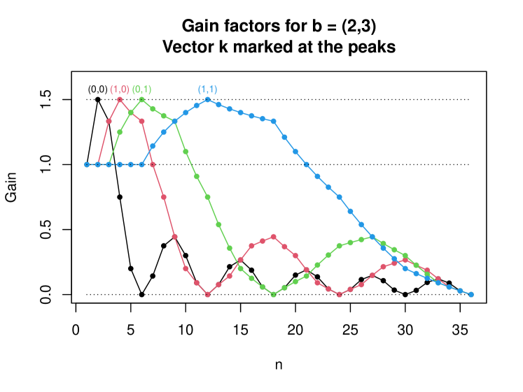
Figure 2: For $d=2$ with $\boldsymbol{b}=(2,3)$ this figure shows the gains for $\boldsymbol{k}\in\{(0,0),(0,1),(1,0),(1,1)\}$ versus $1\leqslant n\leqslant 36$. At $n=36$ all four of these gains are zero. The same peak value $3/2$ attained by all curves. In all cases, the maximum is attained at $n=2\times b_{1}^{k_{1}}\times b_{2}^{k_{2}}$. The horizontal reference lines are at gains $0$, $1$, and $3/2$.

Figure 3 shows gain coefficients for $d=3$ with $\boldsymbol{b}=(2,3,5)$. The values of $n$ range from $1$ to $1000$. Vectors $\boldsymbol{k}$ with $\prod_{j\in u}b_{j}^{k_{j}}>1000$ have gain $1$ for all $n$ in this range. The plot shows gain curves for all other vectors $\boldsymbol{k}$. It is clear that any value of $n$ has a maximal gain close to the overall maximum (empirically $9/8$). In this worst case sense, the scrambled Halton points do not have especially good values of $n$. In another sense, described next, there do exist especially good values of $n$.

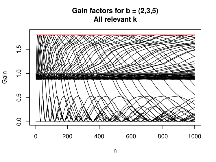
Figure 3: For $d=3$ with $\boldsymbol{b}=(2,3,5)$ this figure shows gain factors $G_{u,\boldsymbol{k}}(n)$ versus $n$ for all non-empty $u\subseteq\{1,2,3\}$ and all $\boldsymbol{k}$ with $\prod_{j\in u}b_{j}^{k_{j}}<n$. For any other $\boldsymbol{k}$ we know that $G_{u,\boldsymbol{k}}(n)=1$ over this range for $n$. There are horizontal reference lines at gains $0$, $1$, and $9/5$.

If we anticipate that smaller values of $|u|$ and of $\prod_{j\in u}b_{j}^{k_{j}}$ correspond to more important features of the function, then values of $n$ that are divisible by products of small powers of the $b_{j}$ have an advantage. We see in Figure 2 that special values of $n$ give gain equal to zero for some of the effects with small $\boldsymbol{k}$. From Figure 3 we can see that selecting such special value of $n$ will not give a meaningful penalty with regard to worst case behavior. This leaves us more free to use convenient or highly composite values of $n$. Values of $n$ that are powers of $10$ are often popular with users. For the Halton sequence, such $n$ are very good for the first and third input dimensions. A value like $n=1800=2^{3}3^{2}5^{2}$ can be expected to give good results when the integrand depends strongly on the first three components of $\boldsymbol{x}$ in a smooth way. A user who wants $n$ to be a power of $10$ might then use bases $2$ and $5$ for what they think are most and second most important input variables, respectively.

A striking feature of Figure 3 is a thick band between gains of 1 and 7/8. The latter value is $G_{1{:}3,\boldsymbol{0}}(2)$. The gains for every $\boldsymbol{k}$ decrease from $1$ to $7/8$ before rising to $9/5$.

In Figures 2 and 3 we never see any $G_{u,\boldsymbol{k}}(n)>\max_{n\in\mathbb{N}}G_{u,\boldsymbol{0}}(n)$. Theorem 1 in Section 5 proves that this can never happen. Theorem 2 in Section 5 shows that if $v\subsetneq u$ then $\sup_{n\geqslant 1}G_{v,\boldsymbol{0}}(n)\leqslant\sup_{n\geqslant 1}G_{u,\boldsymbol{0}}(n)$. Therefore the largest gains for $d$ variables arise in $G_{1:d,\boldsymbol{0}}(n)$ and we only need to consider $n$ from $1$ to $\prod_{j=1}^{d}b_{j}$.

5 Upper bounds for gain

It is of interest to know the largest possible values of gain coefficients. Here, Theorem 1 shows that we only need to consider $\boldsymbol{k}=\boldsymbol{0}$. Then Theorem 2 shows that we only need to consider $u=1{:}d$. Applying Proposition 4, the largest possible gain for $d\geqslant 1$ is one of $G_{1{:}d,\boldsymbol{0}}(n)$ for $1\leqslant n\leqslant\prod_{j=1}^{d}b_{j}$.

Theorem 1.

For all $1\leqslant d<\infty$ and all nonempty $u\subseteq 1{:}d$ and all $\boldsymbol{k}\in\mathbb{N}_{0}^{u}$,

$$\sup_{n\in\mathbb{N}}G_{u,\boldsymbol{k}}(n)=\sup_{n\in\mathbb{N}}G_{u,\boldsymbol{0}}(n).$$ (14)

Proof.

Let $b^{*}=\prod_{j\in u}b_{j}^{k_{j}}$. Corollary 2 shows that

$$G_{u,\boldsymbol{k}}(nb^{*})=G_{u,\boldsymbol{0}}(n).$$ (15)

It suffices to show that for $n^{\prime}$ such that $nb^{*}\leqslant n^{\prime}\leqslant(n+1)b^{*}$, $G_{u,\boldsymbol{k}}(n^{\prime})$ is maximized at the endpoints. That is, we will show that

$$\sup_{nb^{*}\leqslant n^{\prime}\leqslant(n+1)b^{*}}G_{u,\boldsymbol{k}}(n^{\prime})=\max\bigl{(}G_{u,\boldsymbol{k}}(nb^{*}),G_{u,\boldsymbol{k}}((n+1)b^{*})\bigr{)}$$

which is at most $\sup_{n\in\mathbb{N}}G_{u,\boldsymbol{0}}(n)$ by (15). By equations (9) and (11),

$$\widetilde{G}_{u,\boldsymbol{k}}(n^{\prime})=\sum_{v\subseteq u}H_{u,v}m_{u,v,\boldsymbol{k}}\varepsilon_{v}^{\prime}(1-\varepsilon_{v}^{\prime})$$ (16)

where $\varepsilon_{v}^{\prime}=n^{\prime}/m_{u,v,\boldsymbol{k}}-\lfloor n^{\prime}/m_{u,v,\boldsymbol{k}}\rfloor$. We write $n^{\prime}=nb^{*}+r$ for $0\leqslant r\leqslant b^{*}$. Because $m_{u,v,\boldsymbol{k}}=b^{*}m_{u,v,\boldsymbol{0}}$,

$$\varepsilon_{v}^{\prime} =\frac{n^{\prime}}{m_{u,v,\boldsymbol{k}}}-\Bigl{\lfloor}\frac{n^{\prime}}{m_{u,v,\boldsymbol{k}}}\Bigr{\rfloor}$$

$$=\frac{n+r/b^{*}}{m_{u,v,\boldsymbol{0}}}-\Bigl{\lfloor}\frac{n+r/b^{*}}{m_{u,v,\boldsymbol{0}}}\Bigr{\rfloor}$$

$$=\frac{r}{b^{*}m_{u,v,\boldsymbol{0}}}+\frac{n}{m_{u,v,\boldsymbol{0}}}-\Bigl{\lfloor}\frac{n}{m_{u,v,\boldsymbol{0}}}\Bigr{\rfloor}$$

$$=\frac{r}{b^{*}m_{u,v,\boldsymbol{0}}}+\varepsilon_{v}$$

where $\varepsilon_{v}=n/m_{u,v,\boldsymbol{0}}-\lfloor n/m_{u,v,\boldsymbol{0}}\rfloor$. Therefore, the normalized gain coefficients $G_{u,\boldsymbol{k}}(n^{\prime})$ can be expressed as

$$G_{u,\boldsymbol{k}}(n^{\prime}) =\frac{1}{n^{\prime}}\prod_{j\in u}(b_{j}-1)^{-1}\sum_{v\subseteq u}H_{u,v}m_{u,v,\boldsymbol{k}}\varepsilon_{v}^{\prime}(1-\varepsilon_{v}^{\prime})$$

$$=\prod_{j\in u}(b_{j}-1)^{-1}\sum_{v\subseteq u}H_{u,v}\frac{b^{*}m_{u,v,\boldsymbol{0}}}{nb^{*}+r}\varepsilon_{v}^{\prime}(1-\varepsilon_{v}^{\prime})$$

$$=\prod_{j\in u}(b_{j}-1)^{-1}\sum_{v\subseteq u}H_{u,v}\frac{m_{u,v,\boldsymbol{0}}}{n+r/b^{*}}\Bigl{(}\varepsilon_{v}+\frac{r}{b^{*}m_{u,v,\boldsymbol{0}}}\Bigr{)}\Bigl{(}1-\varepsilon_{v}-\frac{r}{b^{*}m_{u,v,\boldsymbol{0}}}\Bigr{)}$$

$$=\prod_{j\in u}(b_{j}-1)^{-1}\sum_{v\subseteq u}H_{u,v}\frac{m_{u,v,\boldsymbol{0}}}{n+x}\biggl{(}\varepsilon_{v}(1-\varepsilon_{v})+(1-2\varepsilon_{v})\frac{x}{m_{u,v,\boldsymbol{0}}}-\frac{x^{2}}{m_{u,v,\boldsymbol{0}}^{2}}\biggr{)}$$

where we have replaced $r/b^{*}$ with $x$. Let us extend the domain of $x$ to all real numbers in $[0,1]$. Our goal becomes to prove that $G_{u,\boldsymbol{k}}(n^{\prime})$, as a function of $x$, is monotonic on $[0,1]$.

First notice that because $H_{u,v}=\prod_{j\in v}b_{j}\prod_{j\in u-v}(-1)=(-1)^{|u-v|}m_{u,v,\boldsymbol{0}}$,

$$\sum_{v\subseteq u}H_{u,v}\frac{m_{u,v,\boldsymbol{0}}}{n+x}\frac{x^{2}}{m_{u,v,\boldsymbol{0}}^{2}}=\frac{x^{2}}{n+x}\sum_{v\subseteq u}(-1)^{|u-v|}=0.$$

This allows us to rewrite $\prod_{j\in u}(b_{j}-1)G_{u,\boldsymbol{k}}(n^{\prime})$ as

$$\sum_{v\subseteq u}H_{u,v}\frac{m_{u,v,\boldsymbol{0}}}{n+x}\Bigl{(}\varepsilon_{v}(1-\varepsilon_{v})+(1-2\varepsilon_{v})\frac{x}{m_{u,v,\boldsymbol{0}}}\Bigr{)}$$

$$= \sum_{v\subseteq u}H_{u,v}m_{u,v,\boldsymbol{0}}\varepsilon_{v}(1-\varepsilon_{v})\frac{1}{n+x}+\sum_{v\subseteq u}H_{u,v}(1-2\varepsilon_{v})\frac{x}{n+x}$$

$$= \frac{1}{n+x}\sum_{v\subseteq u}H_{u,v}\Bigl{(}m_{u,v,\boldsymbol{0}}\varepsilon_{v}(1-\varepsilon_{v})-n(1-2\varepsilon_{v})\Bigr{)}+\sum_{v\subseteq u}H_{u,v}(1-2\varepsilon_{v}).$$

Monotonicity of $G_{u,\boldsymbol{k}}(n^{\prime})$ follows from monotonicity of $1/(n+x)$ on $[0,1]$ and hence $G_{u,\boldsymbol{k}}(n^{\prime})$ is maximized at either endpoint. ∎

Theorem 2.

For all $1\leqslant d<\infty$ and all nonempty $v\subseteq u\subseteq 1{:}d$,

$$\sup_{n\in\mathbb{N}}G_{v,\boldsymbol{0}}(n)\leqslant\sup_{n\in\mathbb{N}}G_{u,\boldsymbol{0}}(n).$$ (17)

Proof.

It suffices to show the conclusion holds when $u-v$ is a single element $j^{*}$ and apply induction. Denote the maximizer of $G_{v,\boldsymbol{0}}(n)$ as $n^{*}$. Our goal is to show that

$$\sup_{n\in\mathbb{N}}G_{v,\boldsymbol{0}}(n)=G_{v,\boldsymbol{0}}(n^{*})\leqslant G_{u,\boldsymbol{0}}(b_{j^{*}}n^{*})\leqslant\sup_{n\in\mathbb{N}}G_{u,\boldsymbol{0}}(n).$$ (18)

For any subset $w\subseteq v$, we define $w_{+}=w\cup\{j^{*}\}$. Then

$$H_{u,w_{+}} =b_{j^{*}}H_{u,w}, H_{u,w} =-H_{v,w},$$ (19)

$$m_{u,w_{+},\boldsymbol{0}} =b_{j^{*}}m_{u,w,\boldsymbol{0}},\quad\text{and}\quad m_{u,w,\boldsymbol{0}} =m_{v,w,\boldsymbol{0}}.$$

We also introduce $K(x)=x(1-x)$ to simplify some expressions. Starting with equation (16) and applying identities from (19), we get for any $n$ divisible by $b_{j^{*}}$ that

$$\widetilde{G}_{u,\boldsymbol{0}}(n) =\sum_{w\subseteq u}H_{u,w}m_{u,w,\boldsymbol{0}}K(\varepsilon_{w})$$

$$=\sum_{w\subseteq v}H_{u,w_{+}}m_{u,w_{+},\boldsymbol{0}}K\biggl{(}\frac{n}{m_{u,w_{+},\boldsymbol{0}}}-\Bigl{\lfloor}\frac{n}{m_{u,w_{+},\boldsymbol{0}}}\Bigr{\rfloor}\biggr{)}$$

$$\quad+\sum_{w\subseteq v}H_{u,w}m_{u,w,\boldsymbol{0}}K\biggl{(}\frac{n}{m_{u,w,\boldsymbol{0}}}-\Bigl{\lfloor}\frac{n}{m_{u,w,\boldsymbol{0}}}\Bigr{\rfloor}\biggr{)}$$

$$=\sum_{w\subseteq v}b^{2}_{j^{*}}H_{v,w}m_{v,w,\boldsymbol{0}}K\biggl{(}\frac{n}{b_{j^{*}}m_{v,w,\boldsymbol{0}}}-\Bigl{\lfloor}\frac{n}{b_{j^{*}}m_{v,w,\boldsymbol{0}}}\Bigr{\rfloor}\biggr{)}$$

$$\quad-\sum_{w\subseteq v}H_{v,w}m_{v,w,\boldsymbol{0}}K\biggl{(}\frac{n}{m_{v,w,\boldsymbol{0}}}-\Bigl{\lfloor}\frac{n}{m_{v,w,\boldsymbol{0}}}\Bigr{\rfloor}\biggr{)}$$

$$=b^{2}_{j^{*}}\widetilde{G}_{v,\boldsymbol{0}}(n/b_{j^{*}})-\widetilde{G}_{v,\boldsymbol{0}}(n).$$ (20)

The corresponding normalized coefficient is

$$G_{u,\boldsymbol{0}}(n) =\frac{1}{b_{j^{*}}n}\prod_{j\in u}(b_{j}-1)^{-1}\Bigl{(}b^{2}_{j^{*}}\widetilde{G}_{v,\boldsymbol{0}}(n/b_{j^{*}})-\widetilde{G}_{v,\boldsymbol{0}}(n)\Bigr{)}$$

$$=\frac{b_{j^{*}}}{(b_{j^{*}}-1)n}\prod_{j\in v}(b_{j}-1)^{-1}\widetilde{G}_{v,\boldsymbol{0}}(n/b_{j^{*}})-\frac{1}{(b_{j^{*}}-1)b_{j^{*}}n}\prod_{j\in v}(b_{j}-1)^{-1}\widetilde{G}_{v,\boldsymbol{0}}(n)$$

$$=\frac{b_{j^{*}}}{b_{j^{*}}-1}G_{v,\boldsymbol{0}}(n/b_{j^{*}})-\frac{1}{b_{j^{*}}-1}G_{v,\boldsymbol{0}}(n).$$

Now, using the fact that $n^{*}$ is the maximizer of $G_{v,\boldsymbol{0}}(n)$

$$G_{u,\boldsymbol{0}}(b_{j^{*}}n^{*}) =\frac{b_{j^{*}}}{b_{j^{*}}-1}G_{v,\boldsymbol{0}}(n^{*})-\frac{1}{b_{j^{*}}-1}G_{v,\boldsymbol{0}}(b_{j^{*}}n^{*})$$

$$\geqslant G_{v,\boldsymbol{0}}(n^{*}).$$

The theorem immediately follows from equation (18). ∎

Theorem 3.

For scrambled Halton points the gains satisfy

$$\sup_{n\in\mathbb{N}}G_{u,\boldsymbol{k}}(n)\leqslant\prod_{j\in u-\{j_{m}\}}\frac{b_{j}}{b_{j}-1}.$$ (21)

for all $d\geqslant 1$, all non-empty $u\subseteq 1{:}d$ and all $\boldsymbol{k}\in\mathbb{N}_{0}^{u}$, where $j_{m}=\arg\min_{j\in u}b_{j}$.

Proof.

According to Theorem 1, it suffices to prove the theorem for $\boldsymbol{k}=\boldsymbol{0}$. Therefore

$$\sup_{n\in\mathbb{N}}G_{u,\boldsymbol{k}}(n)=\sup_{n\in\mathbb{N}}G_{u,\boldsymbol{0}}(n)=\max_{1\leqslant n\leqslant\overline{m}}G_{u,\boldsymbol{0}}(n)$$

where $\overline{m}=\overline{m}_{u,\boldsymbol{0}}=\overline{m}_{u,u,\boldsymbol{0}}=\prod_{j\in u}b_{j}$ and the lower limit $1$ is $\underline{m}_{u,\boldsymbol{0}}=m_{u,\varnothing,\boldsymbol{0}}$.

We proceed by induction on $|u|$. When $u$ only contains a single element $j$, a straightforward calculation shows for $1\leqslant n\leqslant b_{j}$ that

$$G_{u,\boldsymbol{0}}(n)=\frac{b_{j}-n}{b_{j}-1}.$$

So $\sup_{n\in\mathbb{N}}G_{u,\boldsymbol{0}}(n)=G_{u,\boldsymbol{0}}(1)=1$ and the theorem is trivially true for $|u|=1$.

Now for $|u|>1$, we assume that equation (21) holds for $v=u\setminus\{j^{*}\}$ with $j^{*}\neq j_{m}$ and then prove it holds for $u$. From equation (5) and non-negativity of $\widetilde{G}_{v,\boldsymbol{0}}(n)$,

$$\widetilde{G}_{u,\boldsymbol{0}}(n)\leqslant\sum_{w\subseteq v}b_{j^{*}}^{2}H_{v,w}m_{v,w,\boldsymbol{0}}K\biggl{(}\frac{n}{b_{j^{*}}m_{v,w,\boldsymbol{0}}}-\Bigl{\lfloor}\frac{n}{b_{j^{*}}m_{v,w,\boldsymbol{0}}}\Bigr{\rfloor}\biggr{)}.$$

Let $m_{v,w,*}=b_{j^{*}}m_{v,w,\boldsymbol{0}}$ and

$$G_{v,*}(n)=\frac{1}{n}\prod_{j\in v}(b_{j}-1)^{-1}\sum_{w\subseteq v}H_{v,w}m_{v,w,*}K\biggl{(}\frac{n}{m_{v,w,*}}-\Bigl{\lfloor}\frac{n}{m_{v,w,*}}\Bigr{\rfloor}\biggr{)}.$$

We can proceed as in the proof of Theorem 1 with $b^{*}$ replaced by $b_{j^{*}}$ and conclude

$$\sup_{n\in\mathbb{N}}G_{v,*}(n)=\sup_{n\in\mathbb{N}}G_{v,\boldsymbol{0}}(n)\leqslant\prod_{j\in v-\{j_{m}\}}\frac{b_{j}}{b_{j}-1}.$$

Hence

$$G_{u,\boldsymbol{0}}(n) \leqslant\frac{1}{n}\prod_{j\in u}(b_{j}-1)^{-1}\sum_{w\subseteq v}b_{j^{*}}^{2}H_{v,w}m_{v,w,\boldsymbol{0}}K\biggl{(}\frac{n}{b_{j^{*}}m_{v,w,\boldsymbol{0}}}-\Bigl{\lfloor}\frac{n}{b_{j^{*}}m_{v,w,\boldsymbol{0}}}\Bigr{\rfloor}\biggr{)}$$

$$=\frac{b_{j^{*}}}{b_{j^{*}}-1}G_{v,*}(n)$$

$$\leqslant\prod_{j\in u-\{j_{m}\}}\frac{b_{j}}{b_{j}-1}$$

and the theorem follows from induction. ∎

Corollary 3.

For scrambled Halton points in dimension $d\geqslant 1$

$$\sup_{n\geqslant 1}\max_{u\subseteq 1{:}d}\sup_{\boldsymbol{k}\in\mathbb{N}_{0}^{u}}G_{u,\boldsymbol{k}}(n)\leqslant\frac{1}{2}\prod_{j=1}^{d}\frac{b_{j}}{b_{j}-1}.$$

Proof.

The result holds for $d=1$. For $d\geqslant 2$,

$$\sup_{n\geqslant 1}\max_{u\subseteq 1{:}d}\sup_{\boldsymbol{k}\in\mathbb{N}_{0}^{u}}G_{u,\boldsymbol{k}}(n)=\sup_{n\in\mathbb{N}}G_{1{:}d,\boldsymbol{0}}(n)\leqslant\prod_{j=2}^{d}\frac{b_{j}}{b_{j}-1}=\frac{1}{2}\prod_{j=1}^{d}\frac{b_{j}}{b_{j}-1}$$

with the inequality coming from Theorem 3. ∎

Theorem 4.

For the scrambled Halton points

$$\Gamma_{d}=\max_{\varnothing\neq u\subseteq 1{:}d}\sup_{\boldsymbol{k}\in\mathbb{N}_{0}^{u}}\sup_{n\in\mathbb{N}}G_{u,\boldsymbol{k}}(n)=O(\log(d))$$ (22)

as $d\to\infty$.

Proof.

First, $\log(\Gamma_{d})\leqslant\sum_{j=1}^{d}\log(b_{j}/(b_{j}-1))$ where $b_{j}$ is the $j$’th prime number. For any $j\geqslant 1$ we have $b_{j}>\underline{b}_{j}=j\log(j)$ by equation (3.12) of [22]. For any $\epsilon>0$, a Taylor expansion gives

$$\log\Bigl{(}\frac{b_{j}}{b_{j}-1}\Bigr{)}<\log\Bigl{(}\frac{1}{1-1/\underline{b}_{j}}\Bigr{)}<\frac{1}{\underline{b}_{j}}+\frac{1+\epsilon}{2\underline{b}_{j}^{2}}$$

for all $j\geqslant J_{1}=J_{1}(\epsilon)$ for some $J_{1}<\infty$. Then for all large enough $d$, some $J_{2}=J_{2}(\epsilon)\geqslant J_{1}(\epsilon)$ and some constants $c_{\epsilon}<c^{\prime}_{\epsilon}<\infty$

$$\log(\Gamma_{d}) <c_{\epsilon}+\int_{J_{2}-1}^{d}\frac{1}{x\log(x)}\,\mathrm{d}x+\int_{J_{2}-1}^{d}\frac{1+\epsilon}{2(x\log(x))^{2}}\,\mathrm{d}x$$

$$<c^{\prime}_{\epsilon}+\int_{J_{2}-1}^{d}\frac{1}{x\log(x)}\,\mathrm{d}x$$

$$=\log(\log(d))+O(1)$$

as $d\to\infty$. Exponentiating this relationship establishes equation (22). ∎

6 A lower bound

Here we show that the gains cannot be $O(\log(d)^{1-\epsilon})$ for any $\epsilon>0$. First we get a bound for the gain factor of any set $u$ that includes either $j=1$ or $j=2$. This is equivalently about whether either 2 or 3 are among the primes $b_{j}$ for $j\in u$.

Theorem 5.

For $1\leqslant d<\infty$ and $u\subseteq 1{:}d$, if $u\cap\{1,2\}\neq\varnothing$ then

$$\sup_{n\in\mathbb{N}}G_{u,\boldsymbol{k}}(n)\geqslant\prod_{j\in u-\{j^{*}\}}\frac{b_{j}+1}{b_{j}}$$

for any $\boldsymbol{k}\in\mathbb{N}_{0}^{u}$ where $j^{*}$ is any element of $u\cap\{1,2\}$.

Proof of Theorem 5.

According to Theorem 1, it suffices to prove the inequality for $\boldsymbol{k}=\boldsymbol{0}$. For $j^{*}\in u\cap\{1,2\}$, let $b_{*}=b_{j^{*}}$, $n^{*}=\prod_{j\in u,b_{j}\neq b_{*}}b_{j}$ and $V=\{v\subseteq u\mid j^{*}\in v\}$. Because $m_{u,v,\boldsymbol{0}}$ divides $n^{*}$ for any $v\notin V$, $\varepsilon_{v}=n^{*}/m_{u,v,\boldsymbol{0}}-\lfloor n^{*}/m_{u,v,\boldsymbol{0}}\rfloor=0$. Then equation (16) simplifies to

$$\widetilde{G}_{u,\boldsymbol{0}}(n^{*}) =\sum_{v\in V}H_{u,v}m_{u,v,\boldsymbol{0}}K\biggl{(}\frac{n^{*}}{m_{u,v,\boldsymbol{0}}}-\Bigl{\lfloor}\frac{n^{*}}{m_{u,v,\boldsymbol{0}}}\Bigr{\rfloor}\biggr{)}$$

$$=\sum_{v\in V}(-1)^{|u-v|}\biggl{(}\prod_{j\in v}b_{j}^{2}\biggr{)}K\biggl{(}\frac{1}{b_{*}}\prod_{j\in u-v}b_{j}-\Bigl{\lfloor}\frac{1}{b_{*}}\prod_{j\in u-v}b_{j}\Bigr{\rfloor}\biggr{)}$$

where $K(x)=x(1-x)$.

When $b_{*}=2$, because $\prod_{j\in u-v}b_{j}$ is odd,

$$K\biggl{(}\frac{1}{b_{*}}\prod_{j\in u-v}b_{j}-\Bigl{\lfloor}\frac{1}{b_{*}}\prod_{j\in u-v}b_{j}\Bigr{\rfloor}\biggr{)}=K\Bigl{(}\frac{1}{2}\Bigr{)}=\frac{1}{4}.$$

When $b_{*}=3$, because $\prod_{j\in u-v}b_{j}$ an integer not divisible by 3,

$$K\biggl{(}\frac{1}{b_{*}}\prod_{j\in u-v}b_{j}-\Bigl{\lfloor}\frac{1}{b_{*}}\prod_{j\in u-v}b_{j}\Bigr{\rfloor}\biggr{)}=K\Bigl{(}\frac{1}{3}\Bigr{)}=K\Bigl{(}\frac{2}{3}\Bigr{)}=\frac{2}{9}.$$

In either case,

$$K\biggl{(}\frac{1}{b_{*}}\prod_{j\in u-v}b_{j}-\Bigl{\lfloor}\frac{1}{b_{*}}\prod_{j\in u-v}b_{j}\Bigr{\rfloor}\biggr{)}=\frac{b_{*}-1}{b_{*}^{2}}$$

and the normalized coefficient equals

$$G_{u,\boldsymbol{0}}(n^{*}) =\frac{1}{n^{*}}\prod_{j\in u}(b_{j}-1)^{-1}\sum_{v\in V}(-1)^{|u-v|}\biggl{(}\prod_{j\in v}b_{j}^{2}\biggr{)}\frac{b_{*}-1}{b_{*}^{2}}$$

$$=\prod_{j\in u,b_{j}\neq b_{*}}\frac{1}{b_{j}(b_{j}-1)}\sum_{v\in V}(-1)^{|u-v|}\prod_{j\in v,b_{j}\neq b_{*}}b_{j}^{2}$$

$$=\prod_{j\in u,b_{j}\neq b_{*}}\frac{1}{b_{j}(b_{j}-1)}\prod_{j\in u,b_{j}\neq b_{*}}(b_{j}^{2}-1)$$

$$=\prod_{j\in u,b_{j}\neq b_{*}}\frac{b_{j}+1}{b_{j}}.$$

Hence

$$\sup_{n\in\mathbb{N}}G_{u,\boldsymbol{0}}(n)\geqslant G_{u,\boldsymbol{0}}(n^{*})=\prod_{j\in u,b_{j}\neq b^{*}}\frac{b_{j}+1}{b_{j}}.\qed$$

For $d\geqslant 2$ we divide $\prod_{j=1}^{d}(b_{j}+1)/b_{j}$ by either $3/2$ or $4/3$ and still get a lower bound. It follows that

$$\Gamma_{d}\geqslant\frac{3}{4}\prod_{j=1}^{d}\frac{b_{j}+1}{b_{j}}$$

for $j\geqslant 2$, while $\Gamma_{1}=1$.

Corollary 4.

For any $\epsilon>0$

$$\Gamma_{1:d}=\sup_{n\geqslant 1}\max_{u\subseteq 1{:}d}\sup_{\boldsymbol{k}\in\mathbb{N}_{0}^{u}}G_{u,\boldsymbol{k}}(n)$$

cannot be $O((\log d)^{1-\epsilon})$.

Proof.

First $1{:}d\cap\{1,2\}\neq\varnothing$, so Theorem 5 gives $\Gamma_{1:d}\geqslant\prod_{j=2}^{d}(b_{j}+1)/b_{j}$ (which is $1$ for $d=1$). As in the proof of Theorem 4 we note that if $j\geqslant 6$ then $b_{j}<j\log(j)+j\log(\log(j))$. Then for $0<\epsilon^{\prime}<\epsilon^{\prime\prime}<\epsilon$ and large enough $j$

$$\log\Bigl{(}\frac{b_{j}+1}{b_{j}}\Bigr{)}\geqslant\frac{1-\epsilon^{\prime}}{j\log(j)+j\log(\log(j))}\geqslant\frac{1-\epsilon^{\prime\prime}}{j\log(j)}.$$

Using an integral lower bound like the one in the proof of Theorem 5 we get

$$\log(\Gamma_{1:d})\geqslant c+(1-\epsilon^{\prime\prime})\log(\log(d))$$

for some $c\in\mathbb{R}$. After exponentiating, $\Gamma_{1:d}$ cannot be $O((\log d)^{1-\epsilon})$. ∎

7 Conclusions

When we score RQMC methods by their worst case variance relative to plain MC, then we find that scrambled Halton points attain a much better bound than scrambled Sobol’ points do, while retaining the $o(1/n)$ variance property. This does not imply that scrambled Halton points will be generally better than scrambled Sobol’ points in applications, because the integrands of interest may not be ones where scrambled Sobol’ points perform poorly. It does make scrambled Halton points a useful approach for settings where never performing much worse than Monte Carlo is a priority. We note that we could obtain a gain uniformly bounded in $d$ if we were to slightly increase the values $b_{j}$ in use. We do not recommend this as it would be detrimental to the equidistribution properties that QMC and RQMC are designed to produce.

References

- [1] E. Braaten and G. Weller. An improved low-discrepancy sequence for multidimensional quasi-Monte Carlo integration. Journal of Computational Physics, 33(2):249–258, 1979.
- [2] W. Chen, A. Srivastav, and G. Travaglini, editors. A Panorama of Discrepancy Theory. Springer, Cham, Switzerland, 2014.
- [3] S. Da Veiga, F. Gamboa, B. Iooss, and C. Prieur. Basics and Trends in Sensitivity Analysis: Theory and Practice in R. SIAM, Philadelphia, PA, 2021.
- [4] L. Devroye. Non-uniform Random Variate Generation. Springer, 1986.
- [5] J. Dick and F. Pillichshammer. Digital sequences, discrepancy and quasi-Monte Carlo integration. Cambridge University Press, Cambridge, 2010.
- [6] H. Faure. Discrépance de suites associées à un système de numération (en dimension ). Acta Arithmetica, 41:337–351, 1982.
- [7] H. Faure. Good permutations for extreme discrepancy. Journal of Number Theory, 42(1):47–56, 1992.
- [8] H. Faure and C. Lemieux. Generalized Halton sequences in 2008: A comparative study. ACM Transactions on Modeling and Computer Simulation (TOMACS), 19(4):15:1–15:31, 2009.
- [9] J.H. Halton. On the efficiency of certain quasi-random sequences of points in evaluating multi-dimensional integrals. Numerische Mathematik, 2:84–90, 1960.
- [10] F. J. Hickernell. Koksma-Hlawka inequality. Wiley StatsRef: Statistics Reference Online, 2014.
- [11] P. L’Ecuyer and C. Lemieux. A survey of randomized quasi-Monte Carlo methods. In M. Dror, P. L’Ecuyer, and F. Szidarovszki, editors, Modeling Uncertainty: An Examination of Stochastic Theory, Methods, and Applications, pages 419–474. Kluwer Academic Publishers, 2002.
- [12] J. Matoušek. On the L2–discrepancy for anchored boxes. Journal of Complexity, 14:527–556, 1998.
- [13] H. Niederreiter. Point sets and sequences with small discrepancy. Monatshefte fur mathematik, 104(4):273–337, 1987.
- [14] H. Niederreiter. Random Number Generation and Quasi-Monte Carlo Methods. S.I.A.M., Philadelphia, PA, 1992.
- [15] G. Ökten, M. Shah, and Y. Goncharov. Random and deterministic digit permutations of the Halton sequence. In L. Plaskota and H. Woźniakowski, editors, Monte Carlo and Quasi-Monte Carlo Methods 2010, pages 609–622. Springer, 2012.
- [16] A. B. Owen. Randomly permuted -nets and -sequences. In H. Niederreiter and P. J.-S. Shiue, editors, Monte Carlo and Quasi-Monte Carlo Methods in Scientific Computing, pages 299–317, New York, 1995. Springer-Verlag.
- [17] A. B. Owen. Monte Carlo variance of scrambled net quadrature. SIAM Journal on Numerical Analysis, 34(5):1884–1910, 1997.
- [18] A. B. Owen. A randomized Halton algorithm in R. Technical report, arXiv:1706.02808, 2017.
- [19] A. B. Owen. Practical Quasi-Monte Carlo. At https://artowen.su.domains/mc/practicalqmc.pdf, 2023.
- [20] A. B. Owen and Z. Pan. Where are the logs? In Advances in Modeling and Simulation: festschrift for Pierre L’Ecuyer. Springer, Cham, Switzerland, 2022.
- [21] A. B. Owen and D. Rudolf. A strong law of large numbers for scrambled net integration. SIAM Review, 63(2):360–372, 2021.
- [22] J. B. Rosser and L. Schoenfeld. Approximate formulas for some functions of prime numbers. Illinois Journal of Mathematics, 6(1):64–94, 1962.
- [23] Ch. Schlier. A practitioner’s view on QMC integration. Technical report, Universität Freiburg, Fakultät für Physik, 2002.
- [24] I. M. Sobol’. The distribution of points in a cube and the accurate evaluation of integrals (in Russian). Zh. Vychisl. Mat. i Mat. Phys., 7:784–802, 1967.
- [25] B. Vandewoestyne and R. Cools. Good permutations for deterministic scrambled halton sequences in terms of l2-discrepancy. Journal of computational and applied mathematics, 189(1):341–361, 2006.
- [26] X. Wang and F. J. Hickernell. Randomized Halton sequences. Mathematical and Computer Modelling, 32(7-8):887–899, 2000.