Planning to Learn: A Novel Algorithm for Active Learning during Model-Based Planning

Abstract

Active Inference is a recently developed framework for modeling decision processes under uncertainty. Over the last several years, empirical and theoretical work has begun to evaluate the strengths and weaknesses of this approach and how it might be extended and improved. One recent extension is the “sophisticated inference” (SI) algorithm, which improves performance on multi-step planning problems through a recursive decision tree search. However, little work to date has been done to compare SI to other established planning algorithms in reinforcement learning (RL). In addition, SI was developed with a focus on inference as opposed to learning. The present paper therefore has two aims. First, we compare performance of SI to Bayesian RL schemes designed to solve similar problems. Second, we present and compare an extension of SI - sophisticated learning (SL) - that more fully incorporates active learning during planning. SL maintains beliefs about how model parameters would change under the future observations expected under each policy. This allows a form of counterfactual retrospective inference in which the agent considers what could be learned from current or past observations given different future observations. To accomplish these aims, we make use of a novel, biologically inspired environment that requires an optimal balance between goal-seeking and active learning, and which was designed to highlight the problem structure for which SL offers a unique solution. This setup requires an agent to continually search an open environment for available (but changing) resources in the presence of competing affordances for information gain. Our simulations demonstrate that SL outperforms all other algorithms in this context - most notably, Bayes-adaptive RL and upper confidence bound (UCB) algorithms, which aim to solve multi-step planning problems using similar principles (i.e., directed exploration and counterfactual reasoning about belief updates given different possible actions/observations). These results provide added support for the utility of Active Inference in solving this class of biologically-relevant problems and offer added tools for testing hypotheses about human cognition.

*Co-Senior Authors

¹Laureate Institute for Brain Research. Tulsa, OK, USA

²University of Cape Town, South Africa

³University of the Witwatersrand, South Africa

⁴INRS, Montreal, Canada

⁵ Delft University of Technoloty, Department of Cognitive Robotoics

⁶ African Institute for Mathematical Sciences, Muizenberg, Cape Town

⁷South African Astronomical Observatory, Observatory, Cape Town

1 Introduction

Active Inference is a recently proposed framework for modeling decision-making under uncertainty. It shares many features with other prominent decision models, such as Reinforcement Learning (RL), with its main differentiating factors being incorporation of variational inference and an objective function that includes formally derived directed exploration components. To plan, navigate, and learn in task environments, Active Inference agents seek to minimize a quantity called expected free energy (hereafter referred to as EFE within text), instead of simply maximizing reward. As described further in Section 2.1.1, EFE drives agents to choose actions that simultaneously reduce uncertainty about states and model parameters while also maximizing preferred outcomes (e.g., reward).

In recent years, this approach has been compared to traditional decision models within benchmark machine-learning environments. (Friston,, 2009; Sajid et al.,, 2021; Fountas et al.,, 2020; Tschantz et al.,, 2020; Millidge,, 2021). Its performance has been context-dependent, but largely comparable to other algorithms, and many similarities between models have been highlighted. This stems in part from the fact that, although unique, the different information- and reward-seeking terms within EFE have comparable analogues within other agent-based machine learning frameworks. Sajid et al. (2021) have also illustrated how Active Inference aligns with Bayesian Reinforcement Learning when exploration drives are removed. However, particular limitations of Active Inference have also motivated attempts to improve both its performance and tractability. In particular, the scalability of Active Inference remains a significant problem, especially due to the computational cost of variational message passing schemes and policy selection (i.e., policies are typically formulated as pre-defined sets of allowable action sequences). This has led to work integrating Active Inference with other approaches, such as deep learning, neural network architectures, Monte-Carlo Tree search algorithms, and policy gradient objectives (Çatal et al.,, 2020; Fountas et al.,, 2020; Millidge,, 2021).

Another limitation is that standard Active Inference does not maximise reward (i.e., in terms of Bellman optimality) for policy depths greater than one (Da Costa et al.,, 2013). To improve performance in this regard, a ”sophisticated inference” (SI) algorithm has recently been developed. This algorithm is Bellman-optimal and can successfully solve multi-step planning tasks through a recursive tree search (Da Costa et al.,, 2013). However, SI has not yet been rigorously compared to other algorithms, and there are clear directions for its further development. In particular, SI focuses on inference, as opposed to the active learning components of the broader framework.

In this paper, we build on this body of work to achieve two aims. First, we compare Active Inference to other leading algorithms for solving similar problems: Bayes-adaptive reinforcement learning (RL) and upper confidence bound (UCB) approaches. Second, we present and test an extension of SI that incorporates active learning, which we refer to as “sophisticated learning” (SL). To highlight the unique planning process and associated advantages offered by SL, we also compare its performance to the above-mentioned algorithms within a novel, biologically inspired environment that affords multiple directed exploration strategies. Relative performance in this environment clarifies the respective strengths and vulnerabilities of each algorithm. As demonstrated below, SL outperforms all other algorithms tested, and both SL and SI tend to outperform Bayes-adaptive RL (with and without a UCB term).

2 Methods

Below we first review the space of models/algorithms under consideration and their theoretical motivation. We then describe the task environment and the structure of the planning problem that each algorithm was required to solve.

The following variables and notation will be used, which jointly define a partially observable Markov decision process (POMDP):

• $s\in S$ - The external state space upon which the agent performs inference.

• $o\in O$ - The sensory input, or observations, received by the agent.

• $\pi$ - A policy evaluated during planning. In Active Inference, this corresponds to a possible sequence of actions. In RL, this corresponds to a mapping from states to actions.

• $\phi$ - The parameters defining the distribution used by the agent to approximate the true posterior.

• $\theta$ - The parameters that define the generative model.

2.1 Model Space

2.1.1 Standard Active Inference

Active Inference (Friston et al.,, 2011, 2012) proposes that, in partially observable environments with probabilistic state-observation mappings, agents accomplish perception, learning and action selection through minimisation of two respective quantities: variational free energy ($\mathcal{F}$) and expected free energy ($G$). Variational free energy is defined as:

$$\mathcal{F}=\mathbb{E}_{q(s)}\left[\ln{\frac{q(s|o;\phi)}{p(s|o;\theta)}}-\ln{p(o;\theta)}\right]\\$$ (1)

Here, the value of $\mathcal{F}$ will be minimised as the approximate posterior, $q(s|o;\phi)$, approaches the true posterior, $p(s|o;\theta)$. Thus, the agent can approximate optimal state inference (i.e., perception) by finding the distribution $q$ that minimises $\mathcal{F}$. Note that $\mathcal{F}$ will also be minimised as the marginal likelihood, $p(o;\theta)$, approaches a value of one. Thus, the agent can also optimise its model (i.e., learning) by finding the parameters $\theta$ that minimise $\mathcal{F}$.

Action selection in Active Inference is accomplished through minimising $G$, which is the variational free energy of expected future observations (i.e., EFE) under different possible action sequences (policies; $\mathcal{\pi}$) (Parr and Friston,, 2019; Sajid et al.,, 2021). Omitting explicit notation of parameters, this can be defined as:

$$G(\pi) =\mathbb{E}_{q(o,s|\pi)}\left[\ln{\frac{q(s|\pi)}{p(s|o)}}-\ln{p(o)}\right]$$ (2)

$$=\underbrace{-\mathbb{E}_{q(o,s|\pi)}[\ln{p(o|s,\pi)}-\ln{q(o|\pi)}]}_{\text{epistemic value}}]-\underbrace{\mathbb{E}_{q(o|\pi)}[\ln{p(o)}]}_{\text{pragmatic value}}$$

The first line of Equation 2 is nearly equivalent to $\mathcal{F}$ in Equation 1. The important difference is that observations have been included within the expectation. Thus, $G$ calculates the variational free energy of expected future observations. In a POMDP, these expected observations depend on future states, and transitions between states are dependent on the selected policy. The optimal policy will therefore change external states in a way that is expected to generate observations that minimise $G$.

The second line of Equation 2 displays a common decomposition of $G$ with two terms that are integral to the simulations detailed in Section 2.4. The first is the epistemic term. This measures the expected difference between posterior and prior beliefs over states, given a policy. Thus, the larger the expected difference between posterior and prior beliefs, the larger the epistemic value, and, by extension, the smaller the resulting EFE). As its name suggests, the epistemic term therefore measures how much information the agent expects to receive, with a large posterior update meaning that its beliefs have shifted by a proportionally larger amount. Thus, all else being equal, the more state-information a policy is expected to yield, the more an agent will favour that policy. This provides a directed exploration drive that is similar, but not identical, to those often used in RL methods (Mann and Choe,, 2013). An interesting feature of Active Inference is that this term is naturally derived from the free energy formulation, as opposed to the “bootstrapped” heuristics added post-hoc to many RL schemes to promote information-seeking (Pathak et al.,, 2017). Note also that this is a form of state exploration (Schwartenbeck et al.,, 2019). That is, it drives agents to reduce uncertainty about states. This is distinct from active learning drives, which seek to update beliefs about model parameters (sometimes called parameter exploration; discussed further below). This latter form of exploration is more analogous to that used in standard RL (e.g., taking actions to learn about reward probabilities), primarily due to the fact that RL is more often applied in fully observable environments (i.e., MDPs instead of POMDPs).

The second term in the second line of Equation 2 is often referred to as the pragmatic term (Smith et al.,, 2022), though it is also sometimes called the extrinsic value. This term drives the agent to seek out the observations that it prefers or finds most rewarding. This follows from a unique approach to goal-directed choice within Active Inference, in which the prior, $\ln{p(o)}$, is used to encode relative preferences (i.e., observations with higher “probability” are treated as more rewarding). To make this more explicit, it is also sometimes shown as $\ln{p(o|C)}$, where $C$ encodes this fixed set of preferences and is clearly distinct from expected observations under a policy, ${p(o|\pi)}$. All else being equal, the agent can thus be thought of as finding a policy that is expected to minimise the difference between these two distributions.

In addition to the information- and reward-seeking elements just described, Active Inference can also incorporate active learning when there is uncertainty about model parameters. For example, when including beliefs about the parameters of the likelihood function, $\theta$, we have:

$$G(\pi) =\mathbb{E}_{q(o,s,\theta|\pi)}\left[\ln{\frac{q(s,\theta|\pi)}{p(s,\theta|o)}}-\ln{p(o)}\right]$$ (3)

$$=\underbrace{-\mathbb{E}_{q(o,s|\pi)}[\ln{p(s|o,\pi)}-\ln{q(s|\pi)}]}_{\text{epistemic value}}-\underbrace{\mathbb{E}_{q(o,s|\pi)}[D_{kl}(q(\theta|o,s)||q(\theta))}_{\text{novelty}}-\underbrace{\mathbb{E}_{q(o|\pi)}[\ln{p(o)}]}_{\text{pragmatic value}}$$

Here, a new term has been derived that is often referred to as the novelty term. This measures the expected difference between prior and posterior beliefs over model parameters. A posterior belief, in this case, results from the agent updating its model parameters after receiving some observation. As this term is made negative, EFE decreases with greater novelty values. This entails that the agent is driven to sample observations that are expected to cause large changes to its model. In practice, this often equates to the agent preferring states for which observations have been sampled relatively few times, as it is less sure about the parameters encoding $p(o|s)$. Therefore, maximising novelty promotes parameter exploration. This naturally lends itself to effective model learning, as it encourages a “wide” approach to parameter sampling

In models with discrete states and outcomes, the agent’s beliefs about model parameters are typically represented by a Dirichlet distribution, which allows the agent to encode a distribution over its model parameters. A Dirichlet distribution is defined by concentration parameter counts, $\alpha$, which determine the relative probabilities of different parameters. The form of this distribution can be written as:

$$p(\theta|\alpha)=Dir(\theta|\alpha)=\frac{1}{\mathcal{B}(\alpha)}\prod_{i=1}^{k}\theta_{i}^{\alpha_{i}-1}$$ (4)

where $\mathcal{B}$ is a normalising gamma function, and $\alpha_{i}$ is the concentration parameter count for parameter $\theta_{i}$ .

In summary, the EFE functional drives adaptive behaviour by favoring policies that are expected to simultaneously maximise reward (preferred observations) and increase confidence in both states and model parameters. Each of these drives are naturally and dynamically weighted by the magnitude of expected reward and the relative uncertainty about current states and environmental statistics.

2.1.2 Sophisticated Inference (SI)

In the face of the scalability issues of Active Inference mentioned above, an extension to the framework was recently presented by Friston et al. (2021). This method was referred to as Sophisticated Inference (SI), and improves several elements of the original Active Inference algorithm. Firstly, it alleviates the problem of “hard-coded” priors over sets of actions, which act as policies that the agent scores using the EFE functional. SI does this by formulating the EFE as a recursive Bellman equation (conforming to the Bellman optimality principle (Bellman,, 1958)), where inference over states is now conditioned explicitly upon action (and observation) rather than a policy. Thus, defining the action at a given time-step as $u_{t}$, and ignoring the inclusion of model parameter inference for simplicity, EFE in SI takes the following form:

$$G(u_{t},s_{t})= \mathbb{E}_{q(o_{t+1},s_{t+1}|u_{t},s_{t})}[\ln{p(s_{t+1}|o_{t+1},u_{t},s_{t})}-\ln{q(s_{t+1}|u_{t},s_{t}})-\mathbb{E}_{q(o_{t+1})}[\ln{p(o_{t+1})}]$$ (5)

$$+\mathbb{E}_{q(s_{t+1},u_{t+1})}[G(u_{t+1},s_{t+1})]$$

This recursive element, where the EFE of a given action in a state is a function of the EFE, yields a tree-like structure of branching action/state/observation trajectories, with each trajectory weighted by the probability over state-action pairs that constitute it. It is useful to think of these states as belief states because, when the agent simulates this tree-structured look-ahead, it is essentially traversing through beliefs about states rather than actual states. Interpreted psychologically, the agent could here be understood as implementing the following counterfactual thought process:

Based on my current belief about what state I could be in, if I took action $u$ and transitioned to state $s$, what possible observation could I receive, and how would my beliefs about my current state change? Based on this new posterior belief about what hidden states I could be in, what observations would I expect to see if I then took action $u_{t+1}$, and how does that match my preferences?

This is therefore a highly nested, counterfactual belief structure and associated search process. That is, the agent imagines how its beliefs about hidden states would evolve, were it to take certain actions and receive certain observations. Algorithmically, this can be implemented as shown in Figure 1.

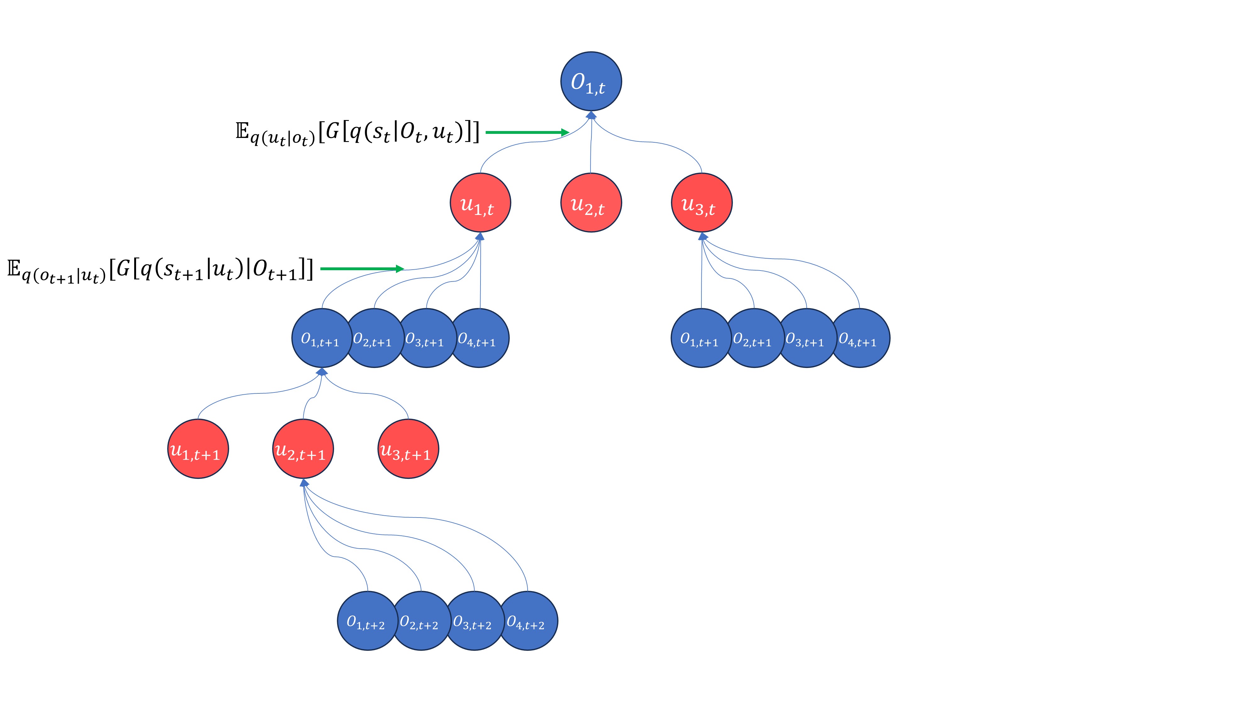
Figure 1: A depiction of the branching recursive search used by the Sophisticated Inference agent. Here, $u$ indicates actions and $O$ indicates observations.

This figure shows the tree-search implemented by an SI agent in order to evaluate trajectories of actions. Here we see that the agent starts with a realised observation, from which, based on its beliefs about hidden states, it implements a simulated trajectory over possible actions, which in turn leads to potential observations, and so on, up to some defined depth of the trajectory. While this process naturally represents an exhaustive search, the algorithm proposed by Friston et al. (2021) incorporates a “pruning” element, whereby a search over specific trajectories of actions and observations is stopped given certain conditions. The first of these conditions is if the prior probability of some future hidden state, given the current belief state and an action, is below some threshold (e.g., set to $p=0.16$ in the original paper). In this case, the occurrence of a transition to such a state is too unlikely, and so the agent disregards it. The second condition that elicits pruning is the case where the EFE of an action is below some relative threshold, when compared to the other possible actions. Similar to the treatment of unlikely states, if this is the case, that action (and the future trajectories it could lead to) is ignored.

Algorithm 1 Sophisticated Inference Tree Search

function ForwardTreeSearch($posterior$, $A$, $a$, $b$, $observation$, $t_{resources}$, $t$, true_t, $T$, $W$, $h$)

     if $t$ $>$ true_t then

         $posterior$ = CalculatePosterior($posterior$, $b$, $a$, $observations$)

         $t_{resources}$ $\leftarrow$ NewTimeSinceResources($posterior(t)$, resource_locations)

     end if

     for each action do

         Q($action$) = b($posterior(t)$, $action$)

         $predicted\_observations$ $\leftarrow$ a(Q($action$)

         $G(action)$ $\leftarrow$ ExpectedFreeEnergy($predicted\_observations$, $t_{resources}$, $W$)

     end for

     if t $<$ $h$ then

         $actions$ $\leftarrow$ ViableActions($G$)

         for $action$ in $actions$ do

              $posterior(t+1)$ $\leftarrow$ Q$(action$)

              $states$ $\leftarrow$ Q($action$)

              $states$ $\leftarrow$ LikelyStates($states$)

              for $state$ in $states$ do

                  $observation$ $\leftarrow$ SampleObservation(state, $a$)

                  [$G$, $posterior$] $\leftarrow$ ForwardTreeSearch($posterior$, $a$, $b$,

                  $observation$, $t_{resources}$, $t+1$, true_t, $T$, $W$, $h$)

                  $S$ $\leftarrow$ softmax($G$) * $G$

                  K($state$) $\leftarrow$ $S$

              end for

              $G$(action) $\leftarrow$ K($states$)*$states$

         end for

     end if

return [$G$, $posterior$]

end function

2.1.3 Bayes-Adaptive Reinforcement Learning

Bayes-adaptive Reinforcement Learning (RL) was chosen as an established algorithm for comparison to SI, as it was developed to solve similar problems in a comparable manner. This approach is situated within the broader paradigm of Bayesian machine learning. To date, considerable investigation has been carried out with respect to Bayesian machine learning, with many such methods emerging as effective ways to incorporate prior information when performing inference over unknown variables (Ghavamzadeh et al.,, 2015). These methods are often applied to problems involving uncertainty, where new information is combined with prior beliefs to formulate posterior beliefs about some unknown factor(s). Of particular relevance here, such methods have been effective in navigating POMDPs (Poupart and Vlassis,, 2008).

These methods either frame POMDPs with respect to uncertainty over the solution-space (model-free), or uncertainty over the parameter-space (model-based). A significant advantage of framing such problems in a Bayesian way is that it effectively side-steps the issue of exploration vs. exploitation. This is due to the fact that Bayesian methods have the capability to represent uncertainty over states/parameters/solutions as belief states. Given, and with respect to, these belief states, optimal solutions can be found (Ghavamzadeh et al.,, 2015). The downside of such an approach is its sensitivity to the initial prior information incorporated into the system, as all belief states are initially entirely based upon this prior (Guez et al.,, 2012). Thus, an integral, and often difficult, aspect of Bayesian Reinforcement Learning is the design and incorporation of effective prior information.

Model-based Bayesian RL offers a particularly interesting approach to modelling uncertainty over parameters. As an example, given a setup where the transition model states $s$ to future states $s^{\prime}$, $p(s^{\prime}|s,a,\theta)$ is unknown, with $\theta$ being the parameters of this transition model, the Bayesian agent can represent this uncertainty with respect to its beliefs about $\theta$.

Given $b\in B$, where $B$ is the belief space and $b(\theta)=Pr(\theta)$, the transition model becomes:

$$p(s^{\prime}|s,b,a)=\int_{\theta}p(s^{\prime}|s,a,\theta)b(\theta)d\theta$$ (6)

Here the expectation of $\theta$ with respect to belief $b$ has been taken (i.e., it has been integrated out), and so $\theta$ does not appear in the resulting probability density. Thus the model is effectively known with respect to belief $b$, and exploration of $\theta$ is not necessary.

Beliefs themselves are updated upon receiving data (in this case data about transitions):

$$b^{\prime}=b(\theta|s,a,s^{\prime})$$ (7)

With the model being framed as known, with respect to $b$, the problem can be formulated as a Markov Decision Process (MDP), and the Bellman equation can be used to determine the optimal value function for each state/belief pair.

$$\upsilon^{*}(s,b)=\operatorname*{arg\,max}_{a}\sum_{s^{\prime},r}p(s^{\prime},r|s,a,b)\left[r+\gamma\upsilon(s^{\prime},b^{s,a,s^{\prime}})\right]\;\;\forall s\in S$$ (8)

As model-based Bayesian RL can be construed as a MDP, it can algorithmically be constructed for any normal model-based RL scheme.

While Bayesian methods offer a principled approach to the exploration/exploitation dilemma, via the construction of a belief-MDP, issues also arise upon the introduction of both model uncertainty and partial observability (Katt et al.,, 2018). In light of these issues, the Bayes-adaptive POMDP framework emerged (Ross et al.,, 2007). As the name suggests, this set of methods uses the foundation of the Bayes-adaptive approach for MDPs (Duff,, 2002) and extends its functionality to the partially observable domain, by allowing the agent to model its own uncertainty over its model of the environment’s dynamics and structure. When navigating a fully observable MDP, an agent can learn by registering and storing the number of times it has witnessed specific environmental dynamics, upon interacting with that environment. As is implied in equation 7, this could take the form of an agent increasing its belief that some state, $s$, transitions to another state, $s^{\prime}$, upon observing the actual occurrence of this specific transition, with its confidence in this transition belief increasing the more such observations it makes. This increase in confidence about a given transition can be represented by incrementing a count, $\mathcal{\phi}^{s^{\prime}}_{sa}$, with the actual belief over parameters, which is implemented as a Dirichlet distribution that uses such counts as its concentration parameters.

However, when operating within a POMDP, the agent does not fully observe the state-space and thus, in many cases, has uncertainty as to what transitions between states actually take place. This creates a scenario where learning is difficult, due to agents in POMDPs often having inaccurate beliefs about the environmental dynamics they sample. To take this uncertainty into account, the Bayes-Adaptive POMDP (BAPOMDP) framework incorporates the agent’s beliefs over model parameters into the hidden state, forming a hyper-state space, $S^{*}=\big{\langle}S,T,\mathcal{O}\big{\rangle}$, with the state-transition and state-observation counts given by $\phi^{s^{\prime}}_{sa}$ and $\theta^{z}_{sa}$ respectively. Thus, the space of $T$ and $\mathcal{O}$ is formally defined as:

$$T=\{\phi\in N^{|S|^{2}|A|}\forall(s,a)\in S\times A,\sum_{s^{\prime}\in S}\phi^{s^{\prime}}_{sa}\}$$

$$\mathcal{O}=\{\theta\in N^{|S|A|Z|}\forall(s,a)\in S\times A,\sum_{z\in Z}\theta^{z}_{sa}\}$$

Therefore, given the definitions $T_{\phi}^{sas^{\prime}}=\frac{\phi^{s^{\prime}}_{sa}}{\sum_{s\neq s^{\prime}}\phi^{s^{\prime}}_{sa}}$ and $\mathcal{O}^{s^{\prime}az}_{\phi}=\frac{\theta^{z}_{sa}}{\sum_{z^{\prime}\neq s^{\prime}}\phi^{z^{\prime}}_{sa}}$, the probabilistic dynamics are given as:

$$p(s^{\prime},\phi^{\prime},\theta^{\prime},z|s,\phi,\theta,a)=T_{\phi}^{sas^{\prime}}\mathcal{O}_{\theta}^{s^{\prime}az}I_{\{\phi^{\prime}\}}(\mathcal{U}(\phi,s,a,s^{\prime}))I_{\{\theta^{\prime}\}}(\mathcal{U}(\theta,s^{\prime},a,z))$$ (9)

where $\mathcal{U}$ is a function that increases the count of $\phi$ and $\theta$ upon the agent receiving data (observations).

While these equations might appear complex, the concept is simple: Given an initial observation and belief over counts $\phi$ and $\theta$, the agent can, in theory, compute all (countably infinite) hyper-states conditioned on this initial belief. Thus, the model becomes known with respect to its priors, with $\mathcal{O}$ and $T$ updated upon the agent receiving new data when interacting with the environment.

While this represents belief states in a POMDP in a mathematically precise way, convergence is only assured with respect to the agent’s initial prior (Katt et al.,, 2018). However, despite this, the framework has shown good convergence properties in practice (Ross et al.,, 2007; Vargo and Cogill,, 2015; Katt et al.,, 2018).

The Bayes-Adaptive learning algorithm used in the simulations described below was online - based on that used by Paquet et al., (2005). The planning structure (search algorithm) is identical to that used in the SI algorithm, with the differences appearing only in the way the reward function is constructed. In general, for these recursive search algorithms, it is important to note that this kind of search exactly equates to a directed value iteration approach, over a subset of reachable states from the initial belief state.

While the preferences in SI are treated as a distribution, the preferences in Bayesian Reinforcement Learning methods are treated as scalar quantities, as is the case in most RL approaches (Sutton and Barto,, 2018). The difference here is that RL views reward as an explicit function that must be optimised, whereas Active Inference methods view reward as the similarity between actual and preferred observations. Although this difference might seem inconsequential, it can sometimes be important, as the nature of the SI preference function being a distribution shapes the resulting scalar values differently (logarithmically, due to the terms of the EFE equation), and allows them to combine proportionally with the values resulting from the evaluation of the epistemic and novelty terms, which are also distribution-based. Standard Bayesian methods, on the other hand, using only scalar numerical values for the reward function, potentially allow for more freedom in how the output of the reward function is shaped, as this shape is not confined to being logarithmic. An example of where this could be particularly useful, over a preference distribution, is in the case where the reward function must be learned - though we do not investigate this here.

Algorithmically, the Bayes-Adaptive method is implemented by simulating searches over the aforementioned hyper-states, which implicitly contain the agent’s uncertainty over model parameters. For the simulations presented below, this essentially means that the UpdateConcentrationParameters update is performed at every recursive step of the ForwardTreeSearch function, rather than only after every real time-step (see pseudo-code below). Importantly, these updates to the concentration parameters, which happen during the forward search, are not carried over to the next real time-step; they exist only within the context of the recursive planning. Like SI, the Bayes-adaptive method implements action and state pruning.

The Bayes-adaptive approach can also be supplemented with an explicit directed exploration term. For optimal comparison to Active Inference, in some simulations below we therefore also add a commonly used directed exploration term - an upper confidence bound (UCB; Agrawal, (1995)) - to Bayes-adaptive RL. Here, UCB takes the form of an algorithmic heuristic which encodes a count over states that an agent has transitioned to up until the current time-point. This can be represented by an expression added to a reward function as follows:

$$reward+c\sqrt{\frac{\ln{(t)}}{N_{t}(a)}}$$ (10)

The following pseudo-code depiction of the Bayes-adaptive RL algorithm incorporates this, with $Nt$ representing the counts of visits to each state up until the current time-point.

Algorithm 2 Bayes-Adaptive Tree Search

function ForwardTreeSearch($posterior$, $A$, $a$, $b$, $observation$, $t_{resources}$, $t$, true_t, $T$, $h$, $N_{t}$)

     if $t$ $>$ true_t then

         $posterior$ = CalculatePosterior($posterior$, $b$, $a$, $observations$)

         $t_{resources}$ $\leftarrow$ NewTimeSinceResources($posterior(t)$, resource_locations)

     end if

     $a,b$ $\leftarrow$ UpdateConcentrationParameters($posterior$, $a$, $b$ o$bservation$)

     for each $action$ do

         Q($action$) = b($posterior(t)$, $action$)

         predicted_observations $\leftarrow$ a(Q($action$)

         R($action$) $\leftarrow$ Reward(predicted_observations, $t_{resources}$, $N_{t}$, Q($action$))

     end for

     if t $<$ $h$ then

         actions $\leftarrow$ ViableActions(R)

         for action in actions do

              $posterior(t+1)$ $\leftarrow$ Q($action$)

              $states$ $\leftarrow$ Q($action$)

              $states$ $\leftarrow$ LikelyStates(states)

              for $state$ in $states$ do

                  $N_{t}$ $\leftarrow$ UpdateStateVisits($N_{t}$, $state$)

                  $observation$ $\leftarrow$ SampleObservation($state$, $a$)

                  [R, $posterior$] $\leftarrow$ ForwardTreeSearch($posterior$, $a$, $b$,

                  $observation$, $t_{resources}$, $t+1$, true_t, $T$, $h$, $N_{t}$)

                  $S$ $\leftarrow$ softmax($R$) * $R$

                  K($state$) $\leftarrow$ $S$

              end for

              R($action$) $\leftarrow$ K($states$)*$states$

         end for

     end if

return [R, $posterior$]

end function

2.2 Sophisticated Learning (SL)

Sophisticated Learning (SL) is a novel algorithm developed here that combines SI with active learning. While SI incorporates epistemic and pragmatic terms of EFE in its recursive tree search (as described in section 2.1.1), it does not incorporate the novelty term in an analogous manner to drive counterfactual parameter exploration. SL essentially combines the SI and Bayes-adaptive methods in a way that harnesses the strengths of both. As shown in section 3 below, it is evident that SI and Bayes-adaptive methods show proportionally worse performance when complex learning is required in dynamic environments. Indeed, while little previous investigation has been done to measure SI’s capability in such environments (Friston et al.,, 2021), it is well established that Bayes-adaptive methods, specifically the BAPOMDP algorithm, are heavily reliant on good initial prior beliefs to implement effective learning (Ross et al.,, 2007; Katt et al.,, 2018). The SL algorithm improves an agent’s ability to perform sophisticated counterfactual reasoning about how its beliefs might evolve, and, in doing so, makes decisions that improve its capacity to learn model parameters.

To create the SL algorithm, the SI scheme was modified to include an update to concentration parameter counts after every time-step, as is the case with the Bayes-adaptive method. This allows SL to propagate beliefs about how parameters would change along its forward tree search. This is important, as it more adequately represents a simulation of how an actual real-time trajectory would unfold if the agent were to really take a particular set of actions and, in doing so, update its model parameters after every step. This simulation is based on the agent’s prior belief over states and parameters, but such techniques have shown good convergence properties (Ross et al.,, 2007).

In addition to this method of counterfactual search, SL also implements a “backwards-smoothing” function - a feature previously suggested (in a more limited scope) in the original presentation of SI (Friston et al.,, 2021). This backwards-smoothing function backtracks from the current time-step to adjust its posterior beliefs over states at previous time-steps. This is particularly useful in the case of learning, as it allows for better matching of observation and state pairs so as to update the Dirichlet concentration parameter counts. The difference in SL, when compared to normal SI schemes, is therefore the addition of both propagating parameter learning through forward-looking simulations, as well as the simulated backward smoothing of parameter learning at every step in this forward search. Psychologically, one could view this as the agent reasoning:

If I were to take an action, receive an observation, and transition to a new belief state, how would I then update my posterior over states for this time-step and for previous time-steps? Based on these posterior updates, how would I then change my current model?

As our results will demonstrate, this method of multi-level counterfactual thinking proves very useful when the likelihood model is unknown in the tested environment (described below).

This backward-smoothing function is specifically given as:

function BackwardsSmoothing($posterior$, $a$, $b$, $observation$, action_history, $t$, $\tau$)

     L $\leftarrow$ posterior

     p $\leftarrow$ $1$

     for $timestep$ = t + 1 to $\tau$ do

         p $\leftarrow$ b(action_history($timestep-1$))$\times$p

         for $state$ in L do

              L($state$) $\leftarrow$ L($state$)$\times$(observation($timestep$))$\times$a$\times$p($state$)

         end for

     end for

return normalise(L)

end function

Integration into the Forward search function was then as follows:

Algorithm 3 Sophisticated Learning Tree Search

function ForwardTreeSearch($posterior$, $A$, $a$, $b$, $observation$, $t_{resources}$, $t$, $true\_t$, $T$, $h$, $backwards\_horizon$, $action\_history$, $resource\_locations$)

     if $t$ $>$ true_t then

         $posterior$ = CalculatePosterior($posterior$, $b$, $a$, $observations$)

         $t_{resources}$ $\leftarrow$ NewTimeSinceResources($posterior(t)$, $resource\_locations$)

     end if

     $start\_time$ $\leftarrow$ $t-backwards_{h}orizon$

     if $start\_time$ $<$ $1$ then

         $start\_time$ $\leftarrow$ $1$

     end if

$novelty$ $\leftarrow$ $0$

     $a\_prior,b\_prior$ $\leftarrow$ $a,b$

     for $\tau$ = $start\_time$ to $t$ do

         L $\leftarrow$ BackwardsSmoothing($posterior$, $a$, $observations$, $action\_history$, $t$, $\tau$)

         $a,b$ $\leftarrow$ UpdateConcentrationParameters($L$, $b$, $observations$, $a$)

     end for

     $W$ $\leftarrow$ CalculateNovelty($a,b,a\_prior,b\_prior$)

     for each action do

         $Q(action)$ = $b(posterior(t),action)$

         $predicted\_observation$s $\leftarrow$ a(Q($action$)

         $G(action)$ $\leftarrow$ ExpectedFreeEnergy($predicted\_observations$, $t_{resources}$, $N_{t}$, $Q(action$))

     end for

     if t $<$ $h$ then

         $actions$ $\leftarrow$ ViableActions(G)

         for $action$ in $actions$ do

              $posterior(t+1)$ $\leftarrow$ Q$(action$)

              $states$ $\leftarrow$ Q($action$)

              $state$s $\leftarrow$ LikelyStates(states)

              for $state$ in $states$ do

                  $observation$ $\leftarrow$ SampleObservation($state$, $a$)

                  [$G$, $posterior$] $\leftarrow$ ForwardTreeSearch($posterior$, $a$, $b$,

                  $observation$, $t_{resources}$, $t+1$, $true\_t$, $T$, $h$, $backwards\_horizon$, $action\_history$, $resource\_locations$)

                  $S$ $\leftarrow$ softmax($G$) * $G$

                  $K(state)$ $\leftarrow$ S

              end for

              $G$($action$) $\leftarrow$ K($states$)*$states$

         end for

     end if

return [$G$, $posterior$]

end function

It is important to note here that the updated concentration parameters are not only passed on to the next recursive call, but are also used to construct (via normalisation) the transition/likelihood functions that are used in subsequent function calls of the recursive search.

2.3 Models Summary

To summarize, the main difference between the recursive Active Inference algorithms (SI and SL) and the Bayes-adaptive algorithm appears in the reward function that is used. Active Inference methods make use of the Expected Free Energy functional, which includes directed state and parameter exploration via the epistemic and novelty terms, respectively. Bayesian RL methods use a reward function based only on preferred outcomes, with no extra exploration heuristics added.

In what follows, we compare these two Active Inference algorithms with Bayes-adaptive RL, both with and without a UCB term (i.e., promoting directed exploration in a manner more analogous to SI and SL).

As a final note: Unlike standard presentations in which parameter values are updated after each trial, our implementation performs these updates after every time step. This was necessary for the agent to solve the problems posed by the environment described below. Thus, all algorithms here operate in a dynamic, “online” manner. In addition, to reduce the number of recursive function calls required, we also employed a commonly used technique called memoization (see Table 1). This technique involves storing, in memory, previous calculations (in this case the expected free energy of a subset of search trajectories) that can be reused when other such search trajectories involve these already-calculated subsets. A drawback to memoization is the significant memory requirement; however, if needed for future applications, this could be solved via various approximation techniques, such as Coarse Coding (Sutton and Barto,, 2018), a form of linear function approximation, or Artificial Neural Networks (Abiodun et al.,, 2018).

2.4 Environment Details and Agent Model

Although a variety of environments have been used to test performance of Active Inference in comparison to other machine learning algorithms (Sajid et al.,, 2021; Millidge,, 2021), these environments have mostly focused on specific elements of classical machine learning behaviour separately, such as exploration, model learning, or reward optimisation. Here we were interested in developing a more demanding environment that would better differentiate performance between the models under consideration and illustrate the unique capabilities of SL. This environment combined the need for dynamically adjusted levels of exploration, parameter learning, and reward optimisation with deep policies and forecasting evolving changes in rewarding outcomes. This was motivated by common problems faced by biological organisms in which: 1) biological needs for resources (e.g., food and water) grow over time at different rates; 2) none of these needs can exceed a threshold to avoid death; and 3) the location of these resources changes over time and requires epistemic foraging.

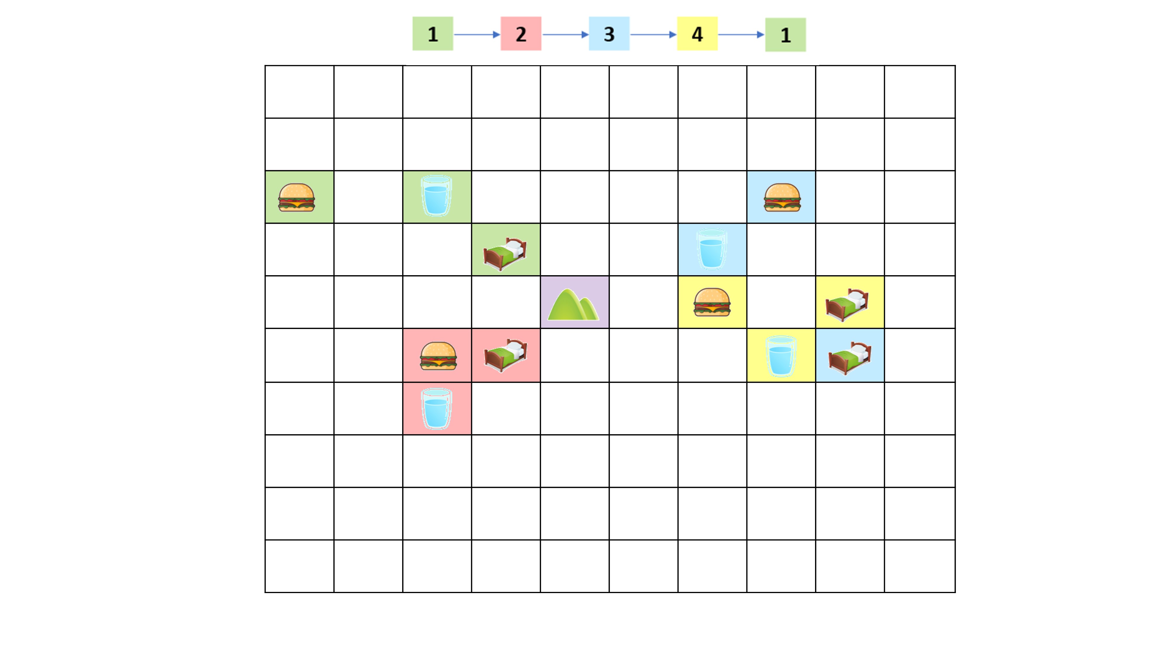
Figure 2: - An example 10-by-10 grid world in one of four different contexts (with different colours representing different seasonal contexts) defining resource locations.

The particular grid world environment in which these demands were implemented is exemplified in Figure 2. Within this environment, there were three categorically-different non-depleting resources that the agent attempted to seek out. The agent was allowed five possible actions per time step: move up, down, left, right, or remain in the same position. The transition function for the positional state, conditioned on these actions, was known by the agent and set to be deterministic. If the agent was at a border of the grid world, any action that would otherwise move it beyond the border instead maintained it in the same position.

The environment also had context states (seasons) that could change over time, where the mapping between positional states and observations (resources) differed for each context state. The context state at a particular time-step was explicitly and fully revealed upon the agent receiving (sampling) an observation given by a particular cue-location state (symbolized as a hill providing a view of the whole environment). It is important to clarify here that while the hill revealed the current context, it did not reveal the position of the resources. This setup posed an explicit explore-exploit dilemma in the context of a POMDP, leading to behavioural patterns taking on three general forms. That is, it would either: 1) sacrifice immediate potential reward and explore positional states for resources, 2) visit the hill to reduce uncertainty about context state, or 3) exploit current beliefs to approach the expected location of each resource directly.

In narrative terms, the goal of the agent in our environment was to seek out and maintain levels for each of three resources - food, water, and sleep - above minimum values for survival, where the locations of these resources were (initially) unknown and probabilistically changed over time (i.e., with different “seasons”). To efficiently learn the locations of these resources, the agent needed to learn their positions in the environment for each respective context/season. This presented a specific challenge, as the agent only ever explicitly knew what season it was in when at the hill state. Thus, it needed to balance moving to resource locations to satiate its needs with visiting the hill to receive information about context (so as to better infer where the resources might be). Over time, if the agent did not move to a resource position, its need for that respective resource would increase - up to a critical point where it would “die” and the iteration would end. This therefore posed a difficult trade-off between information-seeking and reward-seeking.

There were 4 context states: Spring, Summer, Autumn and Winter. At each time-step, each context state probabilistically either remained the same or transitioned to another context (e.g., mimicking a change in seasons). The associated transition probability matrix can be represented as follows (columns = context at time $t$; rows = context at $t+1$):

	Context 1 (Summer)	Context 2 (Spring)	Context 3 (Autumn)	Context 4 (Winter)
Context 1	0.95	0	0	0.05
Context 2	0.05	0.95	0	0
Context 3	0	0.05	0.95	0
Context 4	0	0	0.05	0.95

Along with the two types of states (position and context; implemented as distinct factors), which were explicitly included as part of the agent’s generative model, the agent also registered the number of time-steps it had been without each of the three resources. These measurements functioned as “internal” states of the agent and were not explicitly included in the agent’s generative model (i.e., they were not included as an explicit observation modality). Therefore, the agent, at all time-points, had direct access to these states and did not have to infer them via observations. Despite these internal states not representing formal state factors with modeled transition functions, they did have an implicit transition function known by the agent in all trials. While interesting, we leave questions about uncertainty/inference over internal states to future work.

The hill was always positioned in the middle of the grid world. The agent therefore needed to plan optimal action trajectories to reach the hill, and integrate this with the overarching goal of maintaining sufficient levels of each resource. The initial context state was randomised, with the agent having an initial uniform belief over contexts for all trials. As noted above, and as is apparent in our results, the unique challenges posed by this environment offer key insights into how and why the different algorithms differ in performance.

There were two observation modalities that the agent could receive from the environment. The first consisted of four possible observations: Empty, Food, Water and Sleep. The second observation modality was structured around the context state, with the agent receiving 5 possible observations: Winter, Spring, Summer, Autumn, and a No Context observation, which, as the name suggests, gave the agent no information about the context. The first four observations of this modality were provided by the hill state (depending on the current context), while all other states gave observation 5 (no context). As is often the case with variational Bayesian inference frameworks, the different state factors were factorised as follows, with the likelihood of a context observation given by:

$$p(\textbf{context observation}\;|\;\textbf{positional state},\;\textbf{context state})$$

Algorithm 4, shown below, details how the multi-objective reward function was constructed. Here $resources_{t}$ is the count of time-steps for which the agent has gone without resources, and $resources_{L}$ is the set of time-limits for each resource. Essentially, the agent’s individual preference for each resource increased the longer it had been without that resource. Additionally, as mentioned above, each resource had a distinct time-step limit. If the agent were to go over one of these limits, it would incur a large negative reward (penalty). In the narrative context of our environment, this penalty corresponded to the death of the agent and ended the trial. All transitions to empty squares also incurred a proportionally small negative reward. This multi-objective reward function was structured to be as simple as possible, and follows the forms classically used in Reinforcement Learning grid world environments as follows (Sutton and Barto,, 2018):.

Algorithm 4 Multi-objective reward function

function Preferences($resources_{t}$, $resources_{L}$, penalty)

     $empty_{p}$ $\leftarrow$ -1

     for each resource in [water, food, shelter] do

         $resources_{p}$ $\leftarrow$ $resource_{t}$

         if $resource_{p}$ $\geq$ $resources_{L}$ then

              $empty_{p}$ $\leftarrow$ penalty

              $resources_{p}$ $\neq$ $resource_{L}$ $\leftarrow$ penalty

         end if

     end for

return [$empty_{p},resources_{p}$]

end function

The form of this reward function ultimately results in a dynamic preference distribution. To our knowledge, this feature has not yet been investigated using Active Inference, in which the preference distribution has typically been kept either static or or time-dependent (Tschantz et al.,, 2020; Sajid et al.,, 2021; Friston et al.,, 2021; Smith et al.,, 2022). In contrast, in the simulations presented here, the preference distribution of the agent at any given time-step was a function of the agent’s current internal states (time since each resource). This means that the agent’s future (predicted) preferences were implicitly defined by its own policy. That is, based on the actions it takes, its preferences at each time-step could differ. This created a partially circular structure in which the agent needed to determine a policy that best satisfied the preferences, at each time-step, that the policy itself induced.

The state-space for the environment is formally defined as:

$$position\times food_{t}\times water_{t}\times sleep_{t}\times context$$

Where $food_{t}$, $water_{t}$ and $sleep_{t}$ are the time-steps the agent has gone without each respective resource and $\times$ is the cartesian product. The number of recursive function calls made with and without memoization from $t=1$. Different possible search depths are also included.

Depth	Function calls with memoization	Function calls without memoization
0	1	1
1	17	21
2	53	421
3	117	8421
4	257	160421

Table 1: A comparison of the number of recursive function calls with and without memoization

2.5 Testing and Comparisons

We first confirmed the average length of time each algorithm could successfully survive in the environment when both the transition probabilities (between seasons) and likelihood mapping (resource locations within each season) were known. An analysis of variance (ANOVA) was conducted to assess whether this differed between algorithms.

Subsequent performance comparisons then focused on differences in learning and changes in survival length across trials when the likelihood mapping was unknown (i.e., when the agent knew the seasonal change patterns but needed to learn the resource locations within each season). This scenario was chosen because it provided a unique challenge with competing epistemic and pragmatic affordances. Namely, the agent could visit unknown grid positions to learn resource locations (i.e., parameter exploration, Schwartenbeck et al., (2019)) or go to the hill to reduce uncertainty about the current season (i.e., state exploration), and it was required to balance both of these exploratory drives against the time cost of depleting resources and the need to move efficiently between each resource.

All unknown variables were initialized as flat distributions. Based on preliminary simulations, the value of the primary free parameter - reflecting the precision of the preference distribution - was chosen to promote moderate levels of exploration ($c=0.1$). Note that, when this value is set too high, the epistemic and novelty terms in the expected free energy become effectively down-weighted, which minimizes information-seeking drives. If set too low, the agent is instead insufficiently driven to seek out resources needed for survival.

Testing consisted of 120 cumulative iterations, with each iteration lasting a maximum of 100 time-steps in which the agent could seek out resources and try to survive. An iteration ended when either the agent died (i.e., one of the resources dropped below its threshold value), or the maximum number of time-steps was reached. Based on initial simulations, we heuristically set these thresholds to ensure tractable difficulty without effective removal of the challenge (e.g., where it could, and would, simply wait for resources to return to the same location after a few state transitions).

What the agent learned at the end of each iteration (e.g., when it died or hit the maximum time step) was carried over to the next iteration. This allowed the agent to improve over 120 iterations through cumulative belief updating. Given the high levels of variance in performance (due to the difficulty of the task), this set of 120 iterations was itself repeated 30 times (30 averaged episodes). Results shown in Figure 4 reflect average performance across these 30 repeated episodes of cumulative learning.

The resource time-limits were set as follows:

Time since food limit	Time since water limit	Time since sleep limit
20	22	25

Table 2: The time-limits for each of the respective resources. These were chosen heuristically to allow the agent time to learn the model while also preventing the strategy of simply occupying the resource area of a single context and waiting for that context to periodically return

The simulated scenario, involving known context (season) transitions, but unknown resource positions within each context, is quite challenging for survival and learning. This is, in part, because the context observations given by the hill initially provide no information about resource locations (i.e., the likelihood is unknown). Additionally, the agent must attempt to connect resources it discovers with the current season. However, as the season is stochastically shifting, learning is especially difficult and requires behaviour that most algorithms struggle to achieve (Costa et al.,, 2017).

To formally evaluate significant differences in performance (time-steps survived) between algorithms over time in these simulations, we fit Linear Mixed-Effects models including iteration, algorithm, and their interaction as predictors.

3 Results and Discussion

3.1 Relative Performance

An initial set of 100 repeated simulations showed that, with full knowledge of the environment, each algorithm tended to behave in a similar manner and survived for a similar number of time-steps on average (SL: m = 77.3, sd = 28.1; SI: m = 75.9, sd=29.1; BA: m = 72.6, sd =32.9; BA+UCB: m = 71.3, sd = 32.2). An ANOVA indicated that these survival lengths were not significantly different (F = 0.82, p = 0.486). For reference, the largest numeric difference (between SL and BA+UCB) had a small effect size of Cohen’s d = 0.198.

This overlap in performance was in line with expectations, as the major difference between algorithms pertains to the strategies employed to learn the model. Thus, when the model was already known, each algorithm acted in a similarly “greedy” Bayes-optimal manner. In our simulations, this behaviour typically took the form of first visiting the hill to learn the current season and then moving to the closest resource location for that season (see Figure 3). The agent would then repeatedly move between resource locations in a manner that prioritised those resources expected to be most depleted by time of arrival at their respective locations (i.e., in a forward-looking manner that took into account travel time and individual resource depletion rate). The agent would sometimes also visit the hill again to increase its confidence in where resources might be in future time-steps (i.e., if it was worth checking whether the season might have changed; congruent with Bayes-optimality). Once a resource was unexpectedly absent, the agent would then infer a change in season and move to the closest resource location for the subsequent season (i.e., based on its knowledge of state transitions), and so forth. Thus, all algorithms could successfully exploit knowledge of environmental dynamics and context-dependent resource locations in an efficient manner.

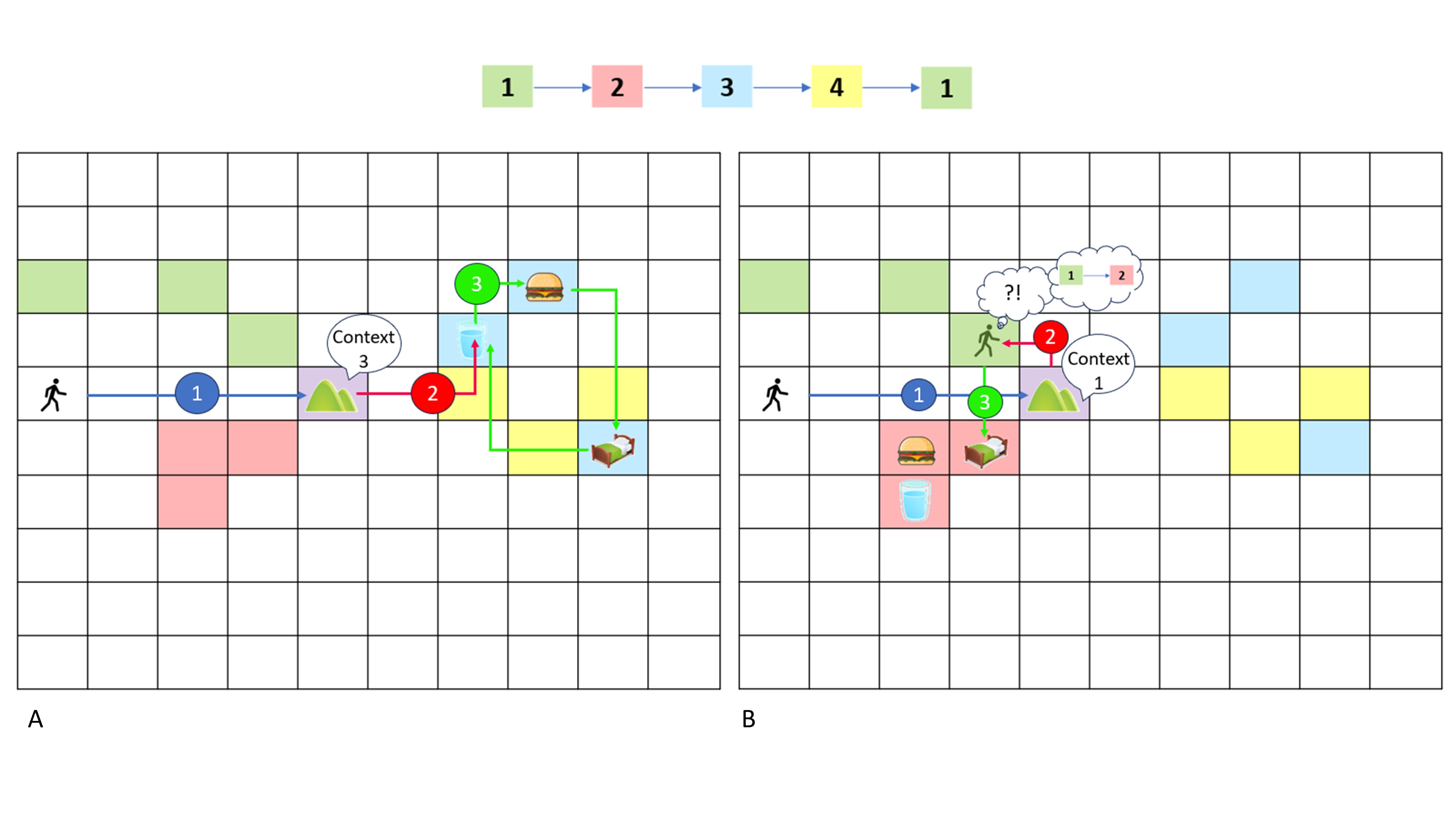
Example behaviour when the full model (transition and likelihood functions) is known, which was similar for all algorithms. (A) The agent would often first visit the hill to determine the season, and then proceed to the nearest position where it knew resources were present in that season. It would subsequently move between known resource positions until it inferred that the season had changed. (B) If the season unexpectedly changes after visiting the hill, the agent may initially be surprised to not find a resource in its expected location. However, because the agent has full knowledge of the environment, it knows what the next season will be, and where the resources are in that new season. Thus, it can leverage this knowledge to move to the new resource locations directly.

Figure 3:

As described in Section 2.5, our primary analyses then compared algorithmic performance in trials where the transition probabilities between seasons were known, but where the likelihood function (i.e., indicating the resource locations within each season) was unknown. Figure 4 depicts the relative performance across iterations for this case.

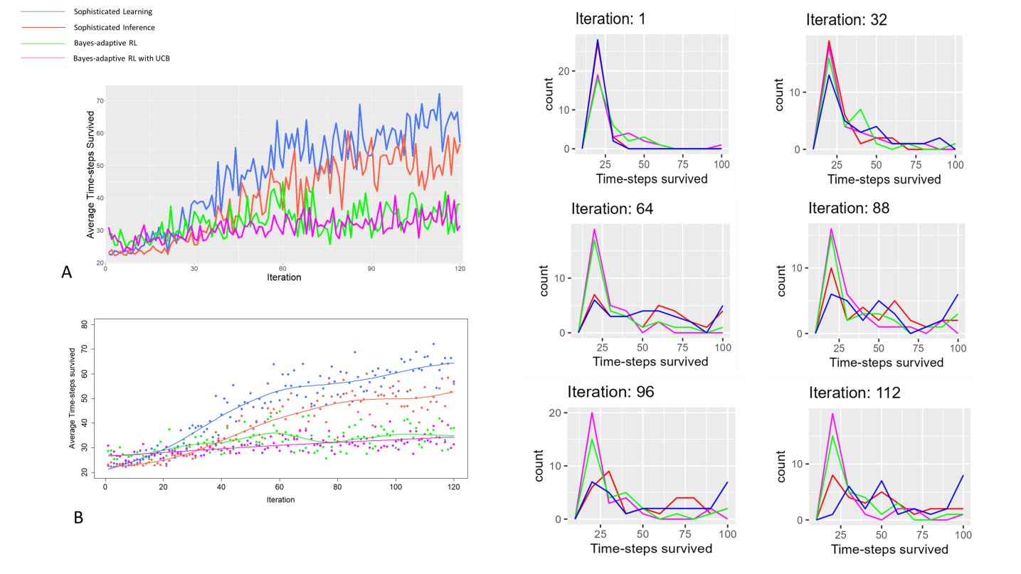
Figure 4: Performance comparison between SL, SI and Bayes-adaptive RL (with or without UCB) averaged over 30 episodes of 120 iterations (with cumulative learning across iterations in each episode). A displays the averaged iterative performance of each algorithm. Here each point is an average of 30 episodes of cumulative learning. B shows a similar display to A, but with a smooth interpolation drawn between averaged points to more clearly illustrate performance differences. C displays frequency counts of time-steps survived for each algorithm. These frequency counts are averaged over 30 episodes for each respective example iteration

As can be seen in Figure 4, SL quickly begins to out-perform SI (at around the 15th iteration). Interestingly, the difference between SL and SI seen at later iterations reflects a significantly larger portion of episodes in which the SL agent survived to the maximum number of time-steps per iteration (100). This was because the SL agent more accurately learned the full likelihood model, and relied less on exploitative behaviour under a partial model. As is also evident in the figure, the Bayes-adaptive algorithms, both with and without UCB, performed quite poorly in comparison and most often survived only a small number of time-steps. This indicates that, in the majority of trials, they were not successful at moving to a correct resource location before dying. This behaviour is characteristic of a “guessing” approach, where the agent would often move to a resource position it thought was closest to its start position and stay there. This behaviour resulted from an imprecise likelihood model.

In formal statistical comparison, linear mixed effects analyses revealed significant main effects of iteration number, algorithm type (model), and their interaction (Iteration: F = 1638.15, p $<$ 0.0001; Model: F = 499.16, p $<$ 0.0001; Iteration*Model: F = 255.70, p $<$ 0.0001). As evident in Figure 4, this interaction was explained by greater improvement in performance over time (iteration) in SL compared to the other algorithms. Indeed, post-hoc comparisons revealed a clear hierarchy of significant differences in degree of improvement. Namely, SL significantly out-performed SI, and both of these algorithms out-performed Bayes-adaptive RL (with and without UCB). The addition of UCB also worsened performance on average (due to over-exploration of locations without resources; see below). Full post-hoc contrast results are displayed in Table 3.

Contrast	Estimate	t-ratio	p-value
SL-SI	7.74	15.86	$<$ 0.0001
SL-BA	15.06	30.84	$<$ 0.0001
SL-BA+UCB	16.92	34.65	$<$ 0.0001
SI-BA	7.31	14.98	$<$ 0.0001
SI-BA+UCB	9.17	18.79	$<$ 0.0001
BA-BA+UCB	1.86	3.8	$<$ 0.0001

Table 3: Post-hoc contrasts derived from a linear mixed-effects analysis on simulation results

3.2 Mechanisms of Differential Performance

Further investigation clarified the mechanisms underlying differential performance between the four algorithms. Note that, in order to accurately learn the likelihood mapping, it was crucial that the agent discover resource positions through random exploration, and then subsequently associate them with a context. In this case, the SL agent showed faster improvement over time because, unlike the other three algorithms, it would often immediately prioritize moving to the hill after discovering a resource. This allowed it to better connect the context (season) with resource location (shown in Figure 5 A). SI learned at a somewhat slower rate, as it did not recognize the hill as a valuable state to visit after discovering a resource. While SI did value the hill state in these simulations, it only did so when either its beliefs about context became sufficiently imprecise, or when the model was precise and the hill became a Bellman-optimal option. Thus, it would not necessarily do so after unexpectedly discovering a resource. Figure 5 B shows example behaviour of an SI agent when finding a resource. Unlike SL, this agent does not prioritize moving to the hill. Instead, it continues to explore surrounding states it has not yet visited, and in general, it visits the hill far less frequently. Learning in this way is relatively slower, as the SI agent, on average, has less precise beliefs about the context in which it has observed a resource. Both Bayes-adaptive algorithms showed very poor learning, as they did not value the hill when their models were imprecise. This is because they did not view the hill as providing a Bellman-optimal mechanism for moving to a resource (as they might if the model were fully known). The logic here is that, if the agent had imprecise beliefs over which context mapped to which resource position, there was no point in learning what the context was before attempting to move to a resource. In the case of Bayes-adaptive RL without UCB, learning was primarily chance-based (i.e., when the agent randomly visited a resource location or visited the hill on the way to some other location it viewed as rewarding). The addition of UCB was also unhelpful. To see why, it is first useful to consider that, while UCB provided a directed exploration drive, this was not goal-directed in the manner displayed by SL. That is, while UCB-driven exploration was directed at states for which the agent had made few observation (i.e., and therefore not random), it was not driven like SL by the goal of precise “credit assignment” of resource locations to a context (i.e., its exploration heuristic did not encourage it to move to the hill to resolve context ambiguity upon discovering a resource). Rather, its exploration was entirely based on relative frequency of states visited over time. In the present environment, which had fairly sparse rewards, this resulted in somewhat “wasteful” over-exploration of states without resources or epistemic value (regarding context).

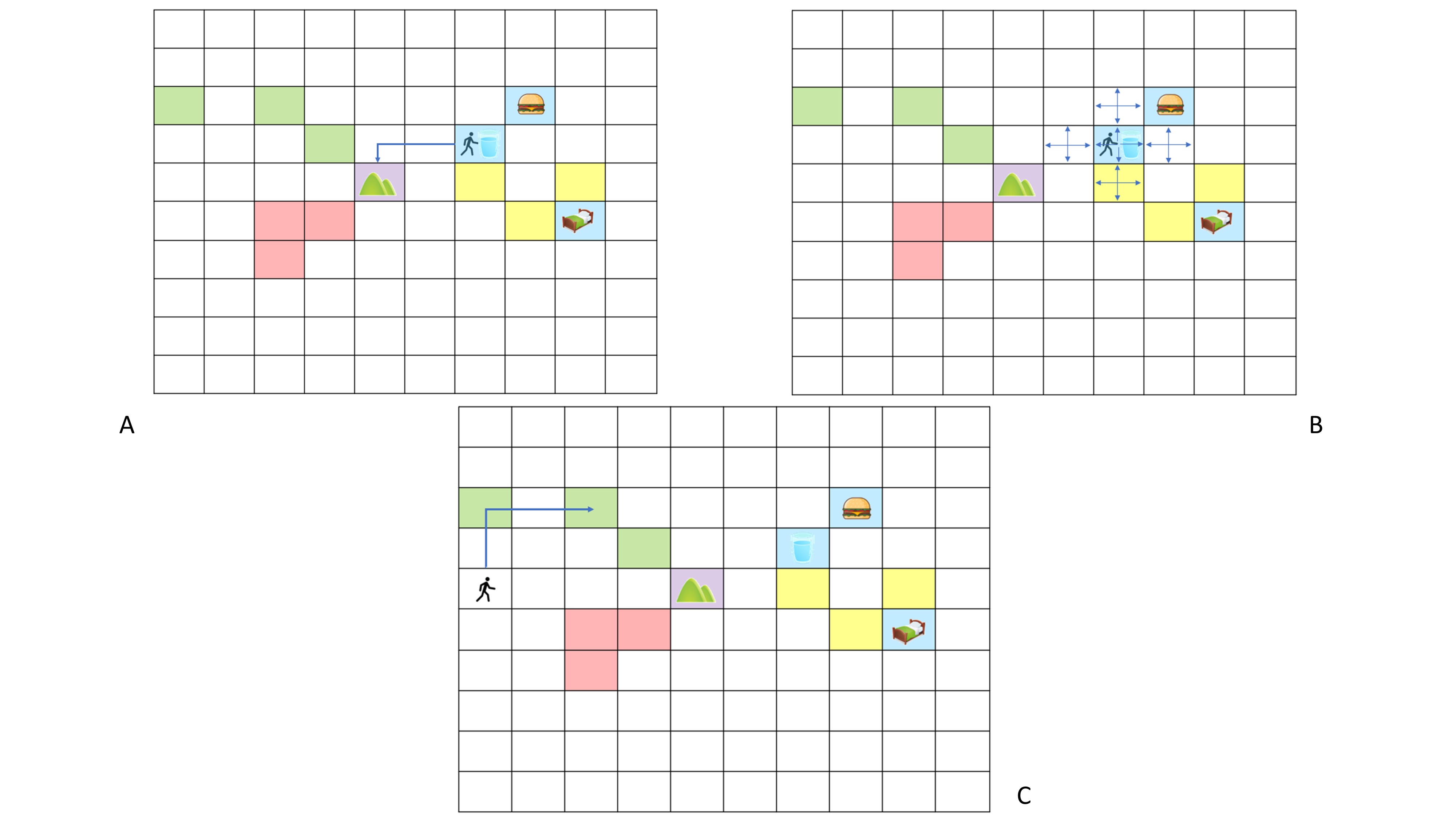
Figure 5: (A) The SL agent frequently visited the hill within a trial to contextualise the information it learned with greater accuracy. (B) The SI agent did not see novelty-based value in the hill, and so did not frequently revisit it to contextualise its prior observations. It instead continued to explore the state-space more broadly to seek out novel observations. (C) Supplementary demonstration of parameter dependence: If the precision of the preference distribution was sufficiently high, both SI and SL agents often ignored the hill and immediately attempted to guess where resources might be (note that, in these simulations, resource locations were known but context was unknown, which further increased the epistemic value of the hill state). This represents an interesting individual difference that might be evaluated in future empirical studies afforded by these models.

3.3 Additional Behavioural Patterns and Parameter Dependence

Single-trial simulations of the two Active Inference algorithms (SI and SL) also revealed interesting patterns of behaviour and dependence on choice of preference precision. As this precision effectively down-weights exploratory drives in the expected free energy, we found that it controlled the total number of time-steps the agent spent at the hill (i.e., resolving uncertainty). For these single-trial simulations, we also examined cases in which resource locations were known but season transitions were not, as we found they provided additional insights regarding parameter dependence. For example, Figure 5 (C) shows a case in which the preference precision was high ($c=1$), the likelihood function known, but the transition function was unknown. In this case, both SI and SL agents, despite lacking information about the current context, initially ignored the hill and attempted to infer the current context by visiting the resource positions it knew were associated with a particular context (due to having a precise likelihood model). This was due to the epistemic term having a proportionally lower impact when compared to the agent’s preferences. Thus, the agent’s behaviour was driven by its drive to meet its multi-objective preferences, rather than to seek information in the form of large posterior updates to its beliefs about hidden states. This is in line with the classic risk-seeking behaviour previously described in the Active Inference literature (Smith et al.,, 2022). For the SI algorithm, similar behaviour was seen when the epistemic term was omitted, regardless of the preference precision.

As mentioned above, when full knowledge of the environment (transition and likelihood functions) was available to any of the four algorithms, similar behaviour was observed, with all algorithms often initially moving to the hill before proceeding to a resource location. This highlights the core similarity between Active Inference and Bayesian RL. That is, both algorithmic paradigms are Bayes-optimal with respect to their prior beliefs, meaning that, given an initial belief state and a mechanism to calculate the value of some subset of additional belief states (for example, all belief states reachable from the initial belief state up to some horizon, as is the case in these implementations), each agent will optimally calculate the value of each of these belief states. Given a deterministic and greedy policy construction procedure, an optimal policy will be chosen that maximises expected value.

Importantly, the accuracy with which these algorithms calculate the value of belief states is entirely predicated on the initial belief state. Thus, if the initial belief state is inaccurate, the calculation and evaluation of subsequent belief states will be inaccurate. Therefore, in simulations where the transition model was known, but the initial context unknown, the agent knew that transitions were relatively static (95% chance to remain in the same context and 5% chance to transition to the next context) and so often viewed visiting the hill as optimal - as it is the state that will most precisely update its belief about what context the environment is in. Due to the nature of the counterfactual trajectory planning these agents implement, they search through all possible belief trajectories up to the planning horizon, and thus calculate, ahead of time, the optimal set of subsequent actions for whatever observation the hill state provides. Planning trajectories then calculate that the hill will provide precise context information, and for each observation the hill could provide, the optimal trajectory following on from that time-point is calculated. These belief trajectories thus have high precision compared to those that do not include the hill.

As briefly mentioned above, behavioural patterns were also influenced by the resource time limits. For example, if one increased the time-limit for each resource compared to the primary simulations above (i.e., 30 time steps without reaching a resource), all agents could initially ignore the hill and simply guess at the context. This was due to the agent not believing that it would incur the penalty of reaching a resource time-limit. Thus, it would lose little by guessing at contexts, even if its guesses were wrong. In these scenarios, the agent would often initially move toward resources based on a guess about the context, and only move to the hill if it believed that subsequent guessing would have a higher chance of incurring death. Mathematically, this is due to the agent precisely following the actions it believed would yield the largest return in the expectation, as is the case with all Bayes-optimal algorithms.

As these parameters (i.e., preference precision, initial belief states, expected resource time limits) influence decision-making in specific ways, this opens up the possibility of using such models in future studies to capture (and mechanistically explain) individual differences in human cognition and behaviour, and potentially their biological basis.

3.4 Summary, Limitations and Conclusion

The overarching aims of this paper have been to: 1) compare performance of the Active Inference paradigm to an established algorithm for solving similar problems (Bayes-adaptive RL), and 2) introduce and compare an extension to SI - sophisticated learning (SL) - that incorporates active learning as well as insights from Bayes-adaptive RL. We performed these comparisons in a biologically inspired, dynamic, multi-objective environment designed to highlight the specific differences between these algorithms. This environment tested the agent’s ability to optimise both exploration and exploitation, as well as effectively learn model parameters in the presence of state-uncertainty. Due to task difficulty, performance showed considerable trial-by-trial variance. However, on average, we found that SI tended to outperform Bayes-adaptive RL, and SL tended to outperform all other algorithms. Performance here was assessed as comparative time-steps survived for each iteration of the trials (which is naturally reliant on accuracy of model learning). Due to the lack of incentive for the RL algorithms to visit a context-disambiguating state (the hill) in these conditions, they showed, on average, poor model learning and performance.

The greater performance shown by SL and SI was due to a sophisticated form of directed exploration not generated by the other algorithms, which allowed for faster learning. In particular, SL was able to take better advantage of (expected) context cues during planning - specifically, returning to the hill after locating a resource to better “link” that resource location to its associated context. This strategic behaviour were due to the unique ability of SL to simulate expected updates in parameters under different action trajectories. Unlike the other algorithms, the SL agent would often return to the hill after locating a resource because it could “imagine” how, in subsequent time-steps, it would look back and update its posterior over context states at previous time-steps with relatively high precision. Therefore, in its look-ahead tree-search, when considering the hill state, it realized that, for whatever observation the hill might generate, it would more precisely update its beliefs about the context in which it was presently observing a resource. Put another way, it understood that, by visiting the hill, it would be able to retrospectively assign a context to the resource location (leading to a more precise anticipated belief update relative to trajectories that would not visit the hill state). Putting a psychological gloss on this mechanism, an agent employing this algorithm might be understood to engage in the following thought process:

I have now discovered a state where a food resource is located. I am unsure of what season I am in at this point, but if I were to move from here and visit the hill state, it would tell me what season I am in. Then, given my transition model, I would be able to work backwards and retrospectively figure out what season I might have been in when I was at the food state. Although not maximally precise, visiting the hill would allow me to do this with more precision than moving to some other state that would not improve my knowledge of what context I am in.

This “thought process” follows from an SL agent’s capacity to propagate its beliefs about how its model parameters would change, were it to receive certain future observations, based on how those observations would affect its beliefs about the current and previous time-steps.

These results suggest that SL offers an important advance in simulating intelligent agent behaviour. In particular, it implements a familiar (human) cognitive process of backward counterfactual reasoning that is not captured by existing algorithms. In contrast, the original SI algorithm was less strategic in its exploratory behaviour; in large part, it simply sought out any states that had not yet been visited. This was due to the more general exploratory drives provided by standard application of the epistemic and novelty terms within the expected free energy. It is this that leads SI to show better performance than Bayesian RL (i.e., which lacks sophisticated information-seeking mechanisms). Interestingly, however, adding a directed exploration (UCB) term to Bayesian RL did not improve performance, and actually led to worse performance due to over-exploration of states with low epistemic affordances about context. This highlights an important distinction between two types of directed exploration. The first, which is present in different forms within SI and UCB, is directed only at states for which few observations have been made. Here, there is no explicit link to a particular goal and can be viewed as a type of intrinsic (but undiscriminating) curiosity. The second, which is present only in SL, is more explicitly goal-directed and strategic in seeking out states expected to improve the agent’s ability to assign observed resource locations to the correct context in its model.

While our results suggest SL is a promising new algorithm, there are several caveats to consider. First, while representing a biologically plausible problem that organisms must solve, the environment was chosen to showcase the unique and advantageous aspects of SL. Future work will be necessary to evaluate the extent to which it facilitates performance in other environments. Given its mathematical properties, we expect it will confer benefits primarily within contexts requiring deep planning and strategic epistemic foraging, as opposed to simpler benchmark environments. Another consideration when applying SL in other environments will be the need to optimise the choice of parameter values. In particular, we expect the optimal value for preference precision will differ when solving different problems. For a given task, a value will need to be identified that does not over- or under-weight the epistemic and novelty terms in the expected free energy to optimise performance.

One further limitation to consider is computational efficiency. At present, as with standard Active Inference, it is not clear how SL can best be scaled up to complex, real-world problems. Therefore, incorporation of other heuristics and machine learning approaches will need to be further investigated, as well as how these might impact the agent’s performance.

To conclude, we have shown, within a challenging dynamic environment requiring strategic information-seeking and complex planning, that Sophisticated Inference outperforms Bayesian RL (with and without additional directed exploration terms), and that an extension of Sophisticated Inference - Sophisticated Learning - offers superior performance and demonstrates categorically distinct, strategic patterns of behaviour. These unique problem-solving strategies emerging from Sophisticated Learning should now be evaluated in other machine learning contexts to assess if they may offer more generalizable advantages. They can now also be assessed within current lines of research in cognitive and computational neuroscience to evaluate the extent to which they capture unique patterns in animal and human behaviour.

Code availability

All code for reproducing and customising the simulations reported in this manuscript can be found at: https://github.com/RowanLIBR/Sophisticated-Learning

Acknowledgment

R.S. is supported by the Laureate Institute for Brain Research and the National Institute of General Medical Sciences (NIGMS; P20GM121312).

References

- Abiodun et al., (2018) Abiodun, O. I., Jantan, A., Omolara, A. E., Dada, K. V., Mohamed, N. A., and Arshad, H. (2018). State-of-the-art in artificial neural network applications: A survey. Heliyon, 4(11).
- Agrawal, (1995) Agrawal, R. (1995). Sample mean based index policies by o (log n) regret for the multi-armed bandit problem. Advances in applied probability, 27(4):1054–1078.
- Bellman, (1958) Bellman, R. (1958). Dynamic programming and stochastic control processes. Information and Control, 1(3):228–239.
- Çatal et al., (2020) Çatal, O., Wauthier, S., Verbelen, T., De Boom, C., and Dhoedt, B. (2020). Deep active inference for autonomous robot navigation. arXiv preprint arXiv:2003.03220.
- Costa et al., (2017) Costa, J., Silva, C., Antunes, M., and Ribeiro, B. (2017). Adaptive learning for dynamic environments: A comparative approach. Engineering Applications of Artificial Intelligence, 65:336–345.
- Da Costa et al., (2013) Da Costa, L., Sajid, N., Parr, T., Friston, K., and Smith, R. (2013). Reward maximization through discrete active inference. Neural Computation, 35(5):807–852.
- Duff, (2002) Duff, M. O. (2002). Optimal Learning: Computational procedures for Bayes-adaptive Markov decision processes. University of Massachusetts Amherst.
- Fountas et al., (2020) Fountas, Z., Sajid, N., Mediano, P., and Friston, K. (2020). Deep active inference agents using monte-carlo methods. Advances in neural information processing systems, 33:11662–11675.
- Friston, (2009) Friston, K. (2009). The free-energy principle: a rough guide to the brain? Trends in Cognitive Sciences, 13(7):293–301.
- Friston et al., (2012) Friston, K., Ao, P., et al. (2012). Free energy, value, and attractors. Computational and mathematical methods in medicine, 2012.
- Friston et al., (2021) Friston, K., Costa, L., Hafner, D., Hesp, C., and Parr, T. (2021). Sophisticated inference. Neural Computation, 33:713–763.
- Friston et al., (2011) Friston, K., Mattout, J., and Kilner, J. (2011). Action understanding and active inference. Biological Cybernetics, 104(1-2):137–160.
- Ghavamzadeh et al., (2015) Ghavamzadeh, M., Mannor, S., Pineau, J., and Tamar, A. (2015). Bayesian reinforcement learning: A survey. Found. Trends Mach. Learn, 8:359–483.
- Guez et al., (2012) Guez, A., Silver, D., and Dayan, P. (2012). Scalable and efficient bayes-adaptive reinforcement learning based on monte-carlo tree search. Journal of Artificial Intelligence Research, 48:841–883.
- Katt et al., (2018) Katt, S., Oliehoek, F., and Amato, C. (2018). Bayesian reinforcement learning in factored pomdps. arXiv preprint arXiv:1811.05612.
- Mann and Choe, (2013) Mann, T. A. and Choe, Y. (2013). Directed exploration in reinforcement learning with transferred knowledge. In Proceedings of the Tenth European Workshop on Reinforcement Learning, volume 24, pages 59–76. PMLR.
- Millidge, (2021) Millidge, B. (2021). Applications of the free energy principle to machine learning and neuroscience. arXiv preprint arXiv:2107.00140.
- Paquet et al., (2005) Paquet, S., Tobin, L., and Chaib-Draa, B. (2005). An online pomdp algorithm for complex multiagent environments. In Proceedings of the fourth international joint conference on Autonomous agents and multiagent systems, pages 970–977.
- Parr and Friston, (2019) Parr, T. and Friston, K. (2019). Generalised free energy and active inference. Biological Cybernetics, 113(5-6):495–513.
- Pathak et al., (2017) Pathak, D., Agrawal, P., Efros, A. A., and Darrell, T. (2017). Curiosity-driven exploration by self-supervised prediction. In Precup, D. and Teh, Y. W., editors, Proceedings of the 34th International Conference on Machine Learning, volume 70, pages 2778–2787. PMLR.
- Poupart and Vlassis, (2008) Poupart, P. and Vlassis, N. (2008). Model-based bayesian reinforcement learning in partially observable domains. In Proc Int. Symp. on Artificial Intelligence and Mathematics,, pages 1–2.
- Ross et al., (2007) Ross, S., Chaib-draa, B., and Pineau, J. (2007). Bayes-adaptive pomdps. Advances in neural information processing systems, 20.
- Sajid et al., (2021) Sajid, N., Ball, P., Parr, T., and Friston, K. (2021). Active inference: Demystified and compared. Neural Comput, 33(3):674–712.
- Schwartenbeck et al., (2019) Schwartenbeck, P., Passecker, J., Hauser, T. U., FitzGerald, T. H., Kronbichler, M., and Friston, K. J. (2019). Computational mechanisms of curiosity and goal-directed exploration. eLife, 8:e41703.
- Smith et al., (2022) Smith, R., Friston, K. J., and Whyte, C. J. (2022). A step-by-step tutorial on active inference and its application to empirical data. Journal of Mathematical Psychology, 107:102632.
- Sutton and Barto, (2018) Sutton, R. and Barto, A. (2018). Reinforcement learning: An introduction.
- Tschantz et al., (2020) Tschantz, A., Millidge, B., Seth, A., and Buckley, C. (2020). Reinforcement learning through active inference. arXiv preprint arXiv:2002.12636.
- Vargo and Cogill, (2015) Vargo, E. P. and Cogill, R. (2015). Expectation-maximization for bayes-adaptive pomdps. Journal of the Operational Research Society, 66(10):1605–1623.