Nonlinear Deterministic Observer for Inertial Navigation using Ultra-wideband and IMU Sensor Fusion

Abstract

Navigation in Global Positioning Systems (GPS)-denied environments requires robust estimators reliant on fusion of inertial sensors able to estimate rigid-body’s orientation, position, and linear velocity. Ultra-wideband (UWB) and Inertial Measurement Unit (IMU) represent low-cost measurement technology that can be utilized for successful Inertial Navigation. This paper presents a nonlinear deterministic navigation observer in a continuous form that directly employs UWB and IMU measurements. The estimator is developed on the extended Special Euclidean Group $\mathbb{SE}_{2}\left(3\right)$ and ensures exponential convergence of the closed loop error signals starting from almost any initial condition. The discrete version of the proposed observer is tested using a publicly available real-world dataset of a drone flight.

I Introduction

Accurate navigation in the absence of Global Positioning Systems (GPS) signals is crucial for various robotics applications such as, autonomous ground vehicles, unmanned aerial vehicles, and autonomous underwater vehicles [1, 2, 3, 4, 5]. Common causes of GPS signal loss are multipath, obstructions, fading, and denial in indoor environments which create the need for a backup navigation solution. In the recent years, a number of GPS-denied navigation solutions have been developed, for instance, vision-aided-based navigation [2, 3, 5, 6] (monocular or stereo camera) and Light Detection and Ranging (LiDAR)-based navigation or 3D laser scanners [1]. However, rapid advances in the areas of Micro-electromechanical systems (MEMS) and communication technology motivates the development of navigation solutions reliant on the fusion of Ultra-wideband (UWB) and Inertial Measurement Unit (IMU) sensors due to their reduced price and weight, and compactness in contrast with other aided navigation units. Moreover, performance of the vision-based techniques degrades in low texture environments, and both vision and LiDAR based systems are costly [4]. Therefore, UWB-IMU fusion could be an optimal fit for inertial navigation of low-cost small-scale vehicles. While IMU enables rigid-body’s orientation estimation, UWB-IMU integration allows for rigid-body’s position and linear velocity estimation. Furthermore, UWB localization is possible with Line-of-sight (LOS) and Non-line-of-sight (NLOS) communication. [7, 8, 9, 10]. However, the main challenge of UWB and IMU technology is high level of measurement uncertainties.

Navigation based on UWB-IMU fusion requires the vehicle to be equipped with UWB tag(s) and a 9-axis IMU (consisting of an accelerometer, a gyroscope, and a magnetometer), along with accessibility of fixed UWB anchors [11]. Since UWB and IMU measurements are uncertain and exclude linear velocity (unlike GPS), a robust observer design is key for the success of control missions. Recently, multiple UWB-IMU-based filters belonging to the family of Kalman filters and Particle Filters (PFs) have been proposed. For instance, a Kalman Filter utilizing smooth set of coordinates compensated under NLOS [7], a Maximum Likelihood Kalman Filtering (MLKF) [10], an extended Kalman filter [11], and an Unscented Kalman Filter (UKF) neglecting the high-order terms [9]. PFs are commonly classified as stochastic filters [12], have been introduced to improve estimation accuracy and address the consistency issue associated with Kalman-type filters. The limitation of the above-mentioned Kalman-type filters [10, 9] is the reliance on linearization around a nominal point ignoring high order nonlinear terms and lowering the estimation accuracy [13]. Moreover, UKF utilizes a set of sigma points complicating filter design and implementation. Meanwhile, PFs are challenged with higher computational cost requirements and lack of a clear measure of optimal performance [13]. Note that state-of-the-art UWB-IMU-based navigation filters rely on Euler angels which are subject to singularities [14] in particular for a rigid-body rotating in three-dimensional (3D) space. Consequently, robust and accurate navigation algorithms for GPS-denied environments remain a challenging open problem.

Contributions

This work aims to frame the navigation kinematics on the Lie group of the extended Special Euclidean Group $\mathbb{SE}_{2}\left(3\right)$. In this work, we consider a vehicle equipped with a 9-axis IMU and at least one UWB tag navigating within the range of fixed UWB anchors. A nonlinear deterministic navigation observer on the Lie group of $\mathbb{SE}_{2}\left(3\right)$ reliant on UWB and IMU measurements is proposed. The proposed observer successfully addresses the unknown bias present in IMU measurements. The proposed observer is tested using a publicly available real-world drone flight dataset [15].

The remainder of the paper is organized as follows: Section II contains preliminaries and mathematical notation. Section III formulates the problem. Section IV introduces the proposed nonlinear navigation observer on $\mathbb{SE}_{2}\left(3\right)$. In Section V, the proposed navigation observer is validated using a real-world drone flight dataset. Finally, Section VI summarizes the work.

II Preliminaries and Math Notation

In this paper, $\mathbb{R}^{a}$, $\mathbb{R}^{a\times b}$, and $\mathbb{R}_{+}$ stands for the set of $a$ dimensional Euclidean space, an $a$-by-$b$ dimensional space, and a set of nonnegative real numbers, respectively. The Euclidean norm of $x\in\mathbb{R}^{n}$ is described by $||x||=\sqrt{x^{\top}x}$ while the Frobenius norm of $M$ is represented by $||M||_{F}=\sqrt{{\rm Tr}\{MM^{*}\}}$ with $*$ referring to a conjugate transpose. The $m$-by-$m$ identity matrix is described by $\mathbf{I}_{n}$ and the $m$-by-$n$ zero matrix is denoted as $0_{n\times m}$. The set of eigenvalues of $M_{r}\in\mathbb{R}^{n\times n}$ is denoted as $\lambda(M_{r})=\{\lambda_{1},\lambda_{2},\ldots,\lambda_{n}\}$. For $M_{r}\in\mathbb{R}^{n\times n}$, $\overline{\lambda}_{M_{r}}=\overline{\lambda}(M_{r})$ and $\underline{\lambda}_{M_{r}}=\underline{\lambda}(M_{r})$ describe the maximum and the minimum eigenvalues of $\lambda(M_{r})$, respectively. For a vehicle navigating with six degrees of freedom (6 DoF), let us denote $\left\{\mathcal{I}\right\}$ as the fixed inertial-frame and $\left\{\mathcal{B}\right\}$ as the fixed body-frame. $\mathbb{SO}\left(3\right)$ denotes the Special Orthogonal Group $\mathbb{SO}\left(3\right)$ where [16, 17]

$$\mathbb{SO}(3)=\{R\in\mathbb{R}^{3\times 3}|R^{\top}R=\mathbf{I}_{3}\text{, }{\rm det}(R)=+1\}$$

with $R\in\mathbb{SO}\left(3\right)$ being rigid-body’s orientation known as attitude. $\mathfrak{so}(3)$ describes the Lie algebra of $\mathbb{SO}(3)$ defined as

$$\mathfrak{so}(3) =\{[y]_{\times}\in\mathbb{R}^{3\times 3}|y\in\mathbb{R}^{3}\}$$

$$\left[y\right]_{\times} =\left[\begin{array}[]{ccc}0&-y_{3}&y_{2}\\ y_{3}&0&-y_{1}\\ -y_{2}&y_{1}&0\end{array}\right]\in\mathfrak{so}\left(3\right),\hskip 10.00002pty=\left[\begin{array}[]{c}y_{1}\\ y_{2}\\ y_{3}\end{array}\right]$$

with $\left[y\right]_{\times}^{\top}=-\left[y\right]_{\times}$ being a skew symmetric matrix. The inverse mapping of $[\cdot]_{\times}$ a 3-dimensional vector ($\mathbf{vex}:\mathfrak{so}\left(3\right)\rightarrow\mathbb{R}^{3}$) defined by

$$\mathbf{vex}([y]_{\times})= y,\forall y\in\mathbb{R}^{3}$$

$$\boldsymbol{\mathcal{P}}_{a}(Y)= \frac{1}{2}(Y-Y^{\top})\in\mathfrak{so}(3),\forall Y\in\mathbb{R}^{3\times 3}$$

and $\mathbf{vex}(\boldsymbol{\mathcal{P}}_{a}(Y))=\frac{1}{2}[Y_{3,2}-Y_{2,3},Y_{1,3}-Y_{3,1},Y_{2,1}-Y_{1,2}]^{\top}\in\mathbb{R}^{3}$. Define the normalized Euclidean distance of $R\in\mathbb{SO}(3)$ as

$$||R||_{{\rm I}}=\frac{1}{4}{\rm Tr}\{\mathbf{I}_{3}-R\}\in\left[0,1\right]$$ (1)

where $-1\leq{\rm Tr}\{R\}\leq 3$. For $M\in\mathbb{R}^{3\times 3}$, $||MR||_{{\rm I}}=\frac{1}{4}{\rm Tr}\{M-MR\}$. For a rigid-body traveling with 6 DoF, let $R\in\mathbb{SO}\left(3\right)$, $P\in\mathbb{R}^{3}$, and $V\in\mathbb{R}^{3}$ denote the rigid-body’s true orientation, position, and velocity, respectively, where $R\in\{\mathcal{B}\}$ and $P,V\in\{\mathcal{I}\}$. Consider the extended form of the Special Euclidean Group $\mathbb{SE}_{2}\left(3\right)=\mathbb{SO}\left(3\right)\times\mathbb{R}^{3}\times\mathbb{R}^{3}\subset\mathbb{R}^{5\times 5}$ [18]

$$\mathbb{SE}_{2}(3) =\{\left.X\in\mathbb{R}^{5\times 5}\right|R\in\mathbb{SO}\left(3\right),P,V\in\mathbb{R}^{3}\}$$ (2)

$$X=\Psi( R,P,V)=\left[\begin{array}[]{ccc}R&P&V\\ 0_{1\times 3}&1&0\\ 0_{1\times 3}&0&1\end{array}\right]\in\mathbb{SE}_{2}\left(3\right)$$ (6)

where $X\in\mathbb{SE}_{2}\left(3\right)$ refers to the homogeneous navigation matrix. Let us define $\Omega\in\mathbb{R}^{3}$, $V\in\mathbb{R}^{3}$, and $a\in\mathbb{R}^{3}$ as the rigid-body’s true angular velocity, linear velocity, and acceleration, respectively, with $\Omega,a\in\{\mathcal{B}\}$. Let us define the submanifold $\mathcal{U}_{\mathcal{M}}=\mathfrak{so}(3)\times\mathbb{R}^{3}\times\mathbb{R}^{3}\times\mathbb{R}\subset\mathbb{R}^{5\times 5}$ as

$$\mathcal{U}_{\mathcal{M}} =\{\left.u([\Omega\text{$]_{\times}$},V,a,\kappa)\right|[\Omega\text{$]_{\times}$}\in\mathfrak{so}(3),V,a\in\mathbb{R}^{3},\varrho\in\mathbb{R}\}$$

$$u( [\Omega\text{$]_{\times}$},V,a,\kappa)=\left[\begin{array}[]{ccc}[\Omega\text{$]_{\times}$}&V&a\\ 0_{1\times 3}&0&0\\ 0_{1\times 3}&\varrho&0\end{array}\right]\in\mathcal{U}_{\mathcal{M}}\subset\mathbb{R}^{5\times 5}$$ (10)

To know more about $\mathbb{SE}_{2}\left(3\right)$ and $\mathcal{U}_{\mathcal{M}}$ visit [2, 5].

III UWB, IMU, and Navigation

The UWB sensors have short wavelength which increases positioning accuracy and their robustness against interference and fading (well-known shortcomings of GPS communication) [8, 9]. UWB sensors are capable of LOS and NLOS communication and obstacle penetration. Furthermore, UWB technology is low in power consumption, compact, and light-weight warranting ease of implementation. Thus, UWB sensors are fit for a positioning system as long as a robust estimation algorithm able to reject uncertainties and produce a reasonable position estimate is employed. UWB positioning can be achieved through various techniques, such as Time Of Arrival (TOA), Angle of Arrival (AOA), Time Difference Of Arrival (TDOA), and Received Signal Strength (RSS) [7, 8]. These approaches are very close in concept. Generally, a UWB tag attached to a vehicle allows to position it using range difference between several Base Stations (BSs) [10]. This work employs the more practical and common TDOA technique. To implement TDOA, let us define $d_{j,i}\in\mathbb{R}$ as the range distance at the UWB tag, and $P=[x,y,z]^{\top}\in\mathbb{R}^{3}$ as the vehicle’s position (with an attached UWB tag). The difference in signals received from the $i$th fixed anchor $h_{i}=[x_{i},y_{i},z_{i}]^{\top}\in\mathbb{R}^{3}$ and the $j$th fixed anchor $h_{j}=[x_{j},y_{j},z_{j}]^{\top}\in\mathbb{R}^{3}$ is defined by

$$d_{j,i}= ||P-h_{j}||-||P-h_{i}||$$ (11)

The equation in (11) can be squared showing that

$$\frac{d_{j,i}^{2}+||h_{i}||^{2}-||h_{j}||^{2}}{2}=(h_{i}-h_{j})^{\top}P-d_{j,i}||P-h_{i}||$$

In view of (11), and considering $N$ TDOA measurements, the following expression can be obtained:

$$\frac{d_{2,1}^{2}+||h_{1}||^{2}-||h_{2}||^{2}}{2}= (h_{1}-h_{2})^{\top}P-d_{2,1}||P-h_{1}||$$

$$\frac{d_{3,2}^{2}+||h_{2}||^{2}-||h_{3}||^{2}}{2}= (h_{2}-h_{3})^{\top}P-d_{3,2}||P-h_{2}||$$

$$\vdots$$

$$\frac{d_{1,N}^{2}+||h_{N}||^{2}-||h_{1}||^{2}}{2}= (h_{N}-h_{1})^{\top}P-d_{1,N}||P-h_{N}||$$ (12)

Considering $||P-h_{3}||=d_{3,2}+||P-h_{2}||$, one finds

$$||P-h_{3}|| =d_{3,2}+d_{2,1}+||P-h_{1}||$$

$$||P-h_{4}|| =d_{4,3}+d_{3,2}+d_{2,1}+||P-h_{1}||$$

As such, for $N$ TDOA measurements, one shows

$$||P-h_{N}|| =\sum_{i=2}^{N}d_{i,i-1}+||P-h_{1}||$$

Define the following matrices

$$A=\left[\begin{array}[]{cc}(h_{1}-h_{2})^{\top}&-d_{2,1}\\ (h_{2}-h_{3})^{\top}&-d_{3,2}\\ \vdots&\vdots\\ (h_{N-1}-h_{N})^{\top}&-d_{N,N-1}\\ (h_{N}-h_{1})^{\top}&-d_{1,N}\end{array}\right]$$

and

$$B=\frac{1}{2}\left[\begin{array}[]{c}d_{2,1}^{2}+||h_{1}||^{2}-||h_{2}||^{2}\\ d_{3,2}^{2}+||h_{2}||^{2}-||h_{3}||^{2}+2d_{3,2}\sum_{i=2}^{2}d_{i,i-1}\\ d_{4,3}^{2}+||h_{3}||^{2}-||h_{4}||^{2}+2d_{4,3}\sum_{i=2}^{3}d_{i,i-1}\\ \vdots\\ d_{1,N}^{2}+||h_{N}||^{2}-||h_{1}||^{2}+2d_{1,N}\sum_{i=2}^{N}d_{i,i-1}\end{array}\right]$$

with $N$ being the number of fixed anchors or BSs accessed by the tag. Hence, one obtains $A\overline{P}-B=0$ where $\overline{P}=[P^{\top},||P-h_{1}||]^{\top}\in\mathbb{R}^{4}$. Thus, by defining $\delta=\frac{1}{2}(AP-B)^{\top}(AP-B)$ and applying minimum mean square error, one obtains $\frac{\partial\delta}{\partial P}=A^{\top}(AP-B)=0$ such that

$$\overline{P}=(A^{\top}A)^{-1}A^{\top}B$$ (13)

where $\overline{P}=[P^{\top},||P-h_{1}||]^{\top}\in\mathbb{R}^{4}$.

Assumption 1.

The rigid-body’s position $P=[x,y,z]^{\top}$ can be uniquely defined in 3D space if at each time instant the tag is within range of at least 4 anchors. Analogously, 3 or more are sufficient to position the rigid-body in 2D space.

The 9-axis IMU consists of three units: a gyroscope, an accelerometer, and a magnetometer [19, 20, 21]. The gyro supplies measurements of rigid-body’s angular velocity expressed as follows:

$$\Omega_{m}=\Omega+b_{\Omega}\in\mathbb{R}^{3}$$ (14)

with $\Omega$ being the true angular velocity and $b_{\Omega}$ referring to unknown bias. The accelerometer provides acceleration measurements:

$$a_{m}=R^{\top}(\dot{V}-\overrightarrow{\mathtt{g}})+b_{a}\in\mathbb{R}^{3}$$ (15)

with $\overrightarrow{\mathtt{g}}=[0,0,g]^{\top}$, $g=-9.8\text{m}/\text{sec}^{2}$ denoting gravitational acceleration, and $\dot{V}$ referring to linear acceleration. $b_{a}$ represents unknown bias. At low frequency, $|\overrightarrow{\mathtt{g}}|>>|\dot{V}|$. Hence, $a_{m}$ can be approximated by $a_{m}\approx-R^{\top}\overrightarrow{\mathtt{g}}+n_{a}$. The magnetometer measurements are defined by

$$m_{m}=R^{\top}m_{r}+b_{m}\in\mathbb{R}^{3}$$ (16)

with $m_{r}=[m_{N},0,m_{D}]^{\top}$ being the earth-magnetic field and $b_{m}$ referring to unknown bias. Three non-collinear observations and measurements are necessary for attitude observation commonly obtained as follows:

$$\begin{cases}v_{1}=\frac{a_{m}}{||a_{m}||},&r_{1}=\frac{-\overrightarrow{\mathtt{g}}}{||-\overrightarrow{\mathtt{g}}||}\\ v_{2}=\frac{m_{m}}{||m_{m}||},&r_{2}=\frac{m_{r}}{||m_{r}||}\\ v_{3}=\frac{v_{1}\times v_{2}}{||v_{1}\times v_{2}||},&r_{3}=\frac{r_{1}\times r_{2}}{||r_{1}\times r_{2}||}\end{cases}$$ (17)

To this end, the true navigation kinematics of a rigid-body traveling with 6 DoF are as follows [2, 6, 5]:

$$\begin{cases}\dot{R}&=R\left[\Omega\right]_{\times}\\ \dot{P}&=V\\ \dot{V}&=Ra+\overrightarrow{\mathtt{g}}\end{cases},\hskip 5.0pt\underbrace{\dot{X}=XU-\mathcal{\mathcal{G}}X}_{\text{Compact form}}$$ (18)

where $R\in\mathbb{SO}\left(3\right)$ stands for the true orientation, $P\in\mathbb{R}^{3}$ describe the true position, $V\in\mathbb{R}^{3}$ expresses the true linear velocity, $\Omega\in\mathbb{R}^{3}$ denotes the true angular velocity, and $a\in\mathbb{R}^{3}$ stands for the acceleration for all $R,\Omega,a\in\{\mathcal{B}\}$ and $P,V\in\{\mathcal{I}\}$. The right part of (18) constitutes the compact form of the navigation kinematics where $X=\Psi(R,P,V)\in\mathbb{SE}_{2}\left(3\right)$ (see the map in (10)), $U=u([\Omega\text{$]_{\times}$},0_{3\times 1},a,1)\in\mathcal{U}_{m}$, and $\mathcal{\mathcal{G}}=u(0_{3\times 3},0_{3\times 1},-\overrightarrow{\mathtt{g}},1)\in\mathcal{U}_{m}$ (see the map in (10)). For more information visit [2].

Lemma 1.

[17] Define $R\in\mathbb{SO}\left(3\right)$, $M_{r}=M_{r}^{\top}\in\mathbb{R}^{3\times 3}$, and consider $\overline{M_{r}}={\rm Tr}\{M_{r}\}\mathbf{I}_{3}-M_{r}$ where $\overline{\lambda}_{\overline{M_{r}}}$ and $\underline{\lambda}_{\overline{M_{r}}}$ stands for the minimum and the maximum eigenvalues of $\overline{M_{r}}$, respectively. Define $||M_{r}R||_{{\rm I}}=\frac{1}{4}{\rm Tr}\{M_{r}(\mathbf{I}_{3}-R)\}$. As such, one obtains:

$$||\mathbf{vex}(\boldsymbol{\mathcal{P}}_{a}(M_{r}R))||^{2} \leq 2\overline{\lambda}_{\overline{M_{r}}}||M_{r}R||_{{\rm I}}$$ (19)

$$||\mathbf{vex}(\boldsymbol{\mathcal{P}}_{a}(M_{r}R))||^{2} \geq\frac{\underline{\lambda}_{\overline{M_{r}}}}{2}||M_{r}R||_{{\rm I}}(1+{\rm Tr}\{R\})$$ (20)

IV Deterministic Navigation Observer

Let us define the estimates of the rigid-body’s orientation, position, and linear velocity as $\hat{R}\in\mathbb{SO}\left(3\right)$, $\hat{P}\in\mathbb{R}^{3}$, and $\hat{V}\in\mathbb{R}^{3}$, respectively. The aim of this section is to propose a nonlinear deterministic navigation observer reliant on UWB-IMU fusion, that drives $\hat{R}\rightarrow R$, $\hat{P}\rightarrow P,$and $\hat{V}\rightarrow V$. Fig. 1 presents a conceptual illustration of the navigation problem, UWB-IMU fusion, and the estimation objective.

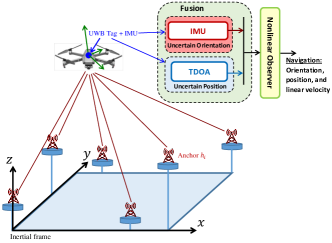
Figure 1: UWB-IMU fusion and navigation estimation problem.

Denote the estimation errors in attitude, position, and linear velocity as $\tilde{R}$ , $\tilde{P}$, and $\tilde{V}$, respectively, and express them as follows:

$$\begin{cases}\tilde{R}&=R\hat{R}^{\top}\\ \tilde{P}&=P-\hat{P}\\ \tilde{V}&=V-\hat{V}\end{cases}$$ (21)

Denote bias estimates of angular velocity and accelerometer as $\hat{b}_{\Omega}$ and $\hat{b}_{a}$, respectively, and express the bias estimation error as follows:

$$\begin{cases}\tilde{b}_{\Omega}&=b_{\Omega}-\hat{b}_{\Omega}\in\mathbb{R}^{3}\\ \tilde{b}_{a}&=b_{a}-\hat{b}_{a}\in\mathbb{R}^{3}\end{cases}$$ (22)

Recalling (17) and define

$$M_{r} =\sum_{i=1}^{3}s_{i}r_{i}r_{i}^{\top},\hskip 10.00002ptM_{B}=\sum_{i=1}^{3}s_{i}v_{i}v_{i}^{\top}$$ (23)

with $s_{i}$ standing for the $i$th sensor confidence level and $\sum_{i=1}^{3}s_{i}=3$. Let us define

$$\hat{v}_{i}=\hat{R}^{\top}r_{i},\hskip 10.00002pt\forall i=1,2,3$$ (24)

Hence, one obtains

$$\mathbf{vex}(\boldsymbol{\mathcal{P}}_{a}(M_{r}\tilde{R})) =\frac{1}{2}\mathbf{vex}(M_{r}\tilde{R}-\tilde{R}^{\top}M_{r})$$

$$=\frac{1}{2}\mathbf{vex}\left(\sum_{i=1}^{3}s_{i}r_{i}v_{i}^{\top}\hat{R}^{\top}-\sum_{i=1}^{3}s_{i}\hat{R}v_{i}r_{i}^{\top}\right)$$

$$=\frac{1}{2}\sum_{i=1}^{3}\hat{R}s_{i}(v_{i}\times\hat{v}_{i})$$ (25)

Note that $[v_{i}\times\hat{v}_{i}]_{\times}=\hat{v}_{i}v_{i}^{\top}-v_{i}\hat{v}_{i}^{\top}$.

Nonlinear observer

Let us introduce the following correction mechanism:

$$\begin{cases}\overline{P}_{y}&=\left[\begin{array}[]{c}P_{y}\\ ||P-h_{1}||\end{array}\right]=(A^{\top}A)^{-1}A^{\top}B\\ \dot{\hat{b}}_{\Omega}&=-\frac{\gamma_{\Omega}}{2}\sum_{i=1}^{n}(v_{i}\times\hat{v}_{i})\\ w_{\Omega}&=-\frac{k_{\Omega}}{2}\sum_{i=1}^{n}\hat{R}(v_{i}\times\hat{v}_{i})\\ w_{V}&=-k_{v}(P_{y}-\hat{P})-[w_{\Omega}]_{\times}\hat{P}\\ w_{a}&=-k_{a}(P_{y}-\hat{P})-[w_{\Omega}]_{\times}\hat{V}\end{cases}$$ (26)

where $\gamma_{\sigma}$, $k_{\Omega}$, $k_{v}$, and $k_{a}$, are positive constants, $v_{i}$ is defined in (17), $v_{i}$ is described in (24), and $P_{y}$ is expressed in (13). Consider the following nonlinear deterministic navigation observer design:

$$\begin{cases}\dot{\hat{R}}&=\hat{R}\left[\Omega_{m}-\hat{b}_{\Omega}\right]_{\times}-\left[w_{\Omega}\right]_{\times}\hat{R}\\ \dot{\hat{P}}&=\hat{V}-\left[w_{\Omega}\right]_{\times}\hat{P}-w_{V}\\ \dot{\hat{V}}&=\hat{R}a_{m}+\overrightarrow{\mathtt{g}}-\left[w_{\Omega}\right]_{\times}\hat{V}-w_{a}\end{cases},\hskip 10.00002pt\underbrace{\dot{\hat{X}}=\hat{X}U_{m}-W\hat{X}}_{\text{Compact form}}$$ (27)

where $w_{\Omega}$, $w_{V}$, and $w_{a}$ are defined in (26). The right part of (27) comprises the compact form of the estimator kinematics where $\hat{X}=\Psi(\hat{R},\hat{P},\hat{V})\in\mathbb{SE}_{2}\left(3\right)$ describes the homogeneous navigation estimate of $X$ (see the map in (6)), $U_{m}=u([\Omega_{m}-\hat{b}_{\Omega}\text{$]_{\times}$},0_{3\times 1},a_{m},1)\in\mathcal{U}_{\mathcal{M}}$, and $W=u([w_{\Omega}\text{$]_{\times}$},w_{V},w_{a},1)\in\mathcal{U}_{\mathcal{M}}$ (see the map in (10)).

Theorem 1.

Consider the nonlinear navigation system in (18). Assume availability of 3 non-collinear measurements/observations and fulfillment of Assumption 1. Let the nonlinear deterministic navigation observer in (27) be coupled with the direct measurements in (13) and the correction terms in (26) such that $\Omega_{m}=\Omega+b_{\Omega}$. Hence, all the closed-loop signals are exponentially stable from almost any initial condition.

Proof.

In view of (18), (21), and (27), one shows

$$\frac{d}{dt}||M_{r}\tilde{R}||_{{\rm I}}= \frac{d}{dt}\frac{1}{4}{\rm Tr}\{M_{r}(\mathbf{I}_{3}-\tilde{R})\}$$

$$= \frac{1}{4}{\rm Tr}\{M_{r}\tilde{R}[\hat{R}\tilde{b}_{\Omega}-w_{\Omega}]_{\times}\}$$

$$= -\frac{1}{2}\mathbf{vex}(\boldsymbol{\mathcal{P}}_{a}(M_{r}\tilde{R}))^{\top}(\hat{R}\tilde{b}_{\Omega}-w_{\Omega})$$ (28)

where $M_{r}$ is a constant matrix and

$${\rm Tr}\{M_{r}\tilde{R}[w_{\Omega}]_{\times}\} ={\rm Tr}\{\boldsymbol{\mathcal{P}}_{a}(M_{r}\tilde{R})[w_{\Omega}]_{\times}\}$$

$$=-\frac{1}{2}\mathbf{vex}(\boldsymbol{\mathcal{P}}_{a}(M_{r}\tilde{R}))^{\top}w_{\Omega}$$

From (18), (21), and (27), one finds

$$\begin{cases}\dot{\tilde{P}}&=\tilde{V}+[w_{\Omega}]_{\times}\hat{P}+w_{V}\\ d\tilde{V}&=(\tilde{R}-\mathbf{I}_{3})\hat{R}a+[w_{\Omega}]_{\times}\hat{V}+w_{a}\end{cases}$$ (29)

Consider the Lyapunov function candidate $\mathcal{L}_{T}=\mathcal{L}_{T}(E_{r},\tilde{P},\tilde{V},\tilde{b}_{\Omega})$:

$$\mathcal{L}_{T}=\mathcal{L}_{R}+\mathcal{L}_{PV}$$ (30)

Define the following Lyapunov function candidate $L_{1}:\mathbb{SO}\left(3\right)\times\mathbb{R}^{3}\rightarrow\mathbb{R}_{+}$:

$$L_{1}=2||M_{r}\tilde{R}||_{{\rm I}}+\frac{1}{2\gamma_{\Omega}}||\tilde{b}_{\Omega}||^{2}$$ (31)

From (31) and (27), one shows

$$\dot{L}_{1} =-\mathbf{vex}(\boldsymbol{\mathcal{P}}_{a}(M_{r}\tilde{R}))^{\top}(\hat{R}\tilde{b}_{\Omega}-w_{\Omega})-\frac{1}{\gamma_{\Omega}}\tilde{b}_{\Omega}^{\top}\dot{\hat{b}}_{\Omega}$$

$$=-k_{\Omega}||\mathbf{vex}(\boldsymbol{\mathcal{P}}_{a}(M_{r}\tilde{R}))||^{2}$$ (32)

$||\mathbf{vex}(\boldsymbol{\mathcal{P}}_{a}(M_{r}\tilde{R}))||\rightarrow 0_{3\times 1}$ shows that $w_{\Omega}\rightarrow 0_{3\times 1}$ and $\dot{\hat{b}}_{\Omega}\rightarrow 0_{3\times 1}$. Hence, $\dot{\tilde{R}}\rightarrow 0_{3\times 3}$ leading to $w_{\Omega}-\hat{R}\tilde{b}_{\Omega}\rightarrow 0_{3\times 1}$, and thereby $\tilde{b}_{\Omega}\rightarrow 0_{3\times 1}$. Since $\boldsymbol{\Upsilon}(M_{r}\dot{R})=\frac{1}{2}({\rm Tr}\{M_{r}R\}\mathbf{I}_{3}-R^{\top}M_{r})\Omega$ [17], define

$$\mathcal{L}_{R}=2||M_{r}\tilde{R}||_{{\rm I}}+\frac{1}{2\gamma_{\Omega}}||\tilde{b}_{\Omega}||^{2}+\frac{\mathbf{vex}(\boldsymbol{\mathcal{P}}_{a}(M_{r}\tilde{R}))^{\top}\hat{R}\tilde{b}_{\Omega}}{2\overline{\gamma}_{\Omega}\overline{\lambda}_{\overline{M_{r}}}}$$

Using (19) one finds

$$e_{R}^{\top}\underbrace{\left[\begin{array}[]{cc}2&-\frac{1}{\overline{\gamma}_{\Omega}}\\ -\frac{1}{\overline{\gamma}_{\Omega}}&\frac{1}{2\gamma_{\Omega}}\end{array}\right]}_{Q_{1}}e_{R}\leq\mathcal{L}_{R}\leq e_{R}^{\top}\underbrace{\left[\begin{array}[]{cc}2&\frac{1}{\overline{\gamma}_{\Omega}}\\ \frac{\delta}{\overline{\gamma}_{\Omega}}&\frac{1}{2\gamma_{\Omega}}\end{array}\right]}_{Q_{2}}e_{R}$$

where $e_{R}=[\sqrt{||M_{r}\tilde{R}||_{{\rm I}}},||\hat{R}\tilde{b}_{\Omega}||]^{\top}$. One shows $\frac{1}{2\overline{\gamma}_{\Omega}\overline{\lambda}_{\overline{M_{r}}}}\frac{d}{dt}(\mathbf{vex}(\boldsymbol{\mathcal{P}}_{a}(M_{r}\tilde{R}))^{\top}\hat{R}\tilde{b}_{\Omega})\leq-\frac{\sqrt{3}}{4\overline{\gamma}_{\Omega}}||\tilde{b}_{\Omega}||^{2}+c_{1}||\boldsymbol{\Upsilon}(M_{r}\tilde{R})||^{2}+c_{2}||\boldsymbol{\Upsilon}(M_{r}\tilde{R})||\,||\tilde{b}_{\Omega}||$ where $c_{1}=\frac{\gamma_{\Omega}}{2\overline{\gamma}_{\Omega}\overline{\lambda}_{\overline{M_{r}}}}|$ and $c_{2}=\frac{\sqrt{3}k_{\Omega}+c_{\Omega}}{2\overline{\gamma}_{\Omega}\overline{\lambda}_{\overline{M_{r}}}}$. Consequently,

$$\dot{\mathcal{L}}_{R}\leq -(k_{\Omega}-c_{1})||\boldsymbol{\Upsilon}(M_{r}\tilde{R})||^{2}-\frac{\sqrt{3}}{4\overline{\gamma}_{\Omega}}||\tilde{b}_{\Omega}||^{2}$$

$$+c_{2}||\boldsymbol{\Upsilon}(M_{r}\tilde{R})||\,||\tilde{b}_{\Omega}||$$ (33)

Recalling (20), one finds

$$\dot{\mathcal{L}}_{R}\leq -e_{R}^{\top}\underbrace{\left[\begin{array}[]{cc}\frac{k_{\Omega}-c_{1}}{c_{R}}&-c_{2}\overline{\lambda}_{\overline{M_{r}}}\\ -c_{2}\overline{\lambda}_{\overline{M_{r}}}&\frac{\sqrt{3}}{4\overline{\gamma}_{\Omega}}\end{array}\right]}_{Q_{2}}e_{R}$$ (36)

$$\mathcal{L}_{R}\leq \mathcal{L}_{R}(0)\exp(-\underline{\lambda}_{Q_{3}}t/\overline{\lambda}_{Q_{2}})$$ (37)

where $c_{R}=\frac{\underline{\lambda}_{\overline{M_{r}}}}{2}(1+{\rm Tr}\{\tilde{R}(0)\})$ and $Q_{2}$ is made positive by selecting $k_{\Omega}>\frac{4c_{R}\overline{\gamma}_{\Omega}c_{2}^{2}\overline{\lambda}_{\overline{M_{r}}}^{2}}{\sqrt{3}}+c_{1}$. Define the following real value function:

$$\mathcal{L}_{PV}= \frac{1}{2}||\tilde{P}||^{2}+\frac{1}{2k_{a}}||\tilde{V}||^{2}-\delta\tilde{P}^{\top}\tilde{V}$$ (38)

$$e_{PV}^{\top}\underbrace{\left[\begin{array}[]{cc}\frac{1}{2}&-\frac{\delta}{2}\\ -\frac{\delta}{2}&\frac{1}{2k_{a}}\end{array}\right]}_{Q_{4}}e_{PV}\leq\mathcal{L}_{PV}\leq e_{PV}^{\top}\underbrace{\left[\begin{array}[]{cc}\frac{1}{2}&\frac{\delta}{2}\\ \frac{\delta}{2}&\frac{1}{2k_{a}}\end{array}\right]}_{Q_{5}}e_{PV}$$

where $e_{PV}=[||\tilde{P}||,||\tilde{V}||]^{\top}$. Hence, using (29) and (38), one obtains

$$\dot{\mathcal{L}}_{PV}\leq -(k_{v}-\delta k_{a})||\tilde{P}||^{2}-\delta||\tilde{V}||^{2}+\delta k_{v}||\tilde{V}||\,||\tilde{P}||$$

$$+(\delta||\tilde{P}||+\frac{1}{k_{a}}||\tilde{V}||)||\mathbf{I}_{3}-\tilde{R}||_{F}\hat{R}a$$ (39)

where $c_{a}=\max\{\sup_{t\geq 0}4\delta\overline{\lambda}_{M}a,\sup_{t\geq 0}\frac{4\overline{\lambda}_{M}a}{k_{a}}\}$, $||{\rm Tr}\{M_{r}\tilde{R}\}\mathbf{I}_{3}-M_{r}\tilde{R}||_{F}\leq\sqrt{3}\overline{\lambda}_{\overline{M_{r}}}$. Thus, $\dot{\mathcal{L}}_{PV}$ in (39) becomes

$$\dot{\mathcal{L}}_{PV}\leq -e_{PV}^{\top}\underbrace{\left[\begin{array}[]{cc}k_{v}-\delta k_{a}&-\frac{\delta k_{v}}{2}\\ -\frac{\delta k_{v}}{2}&\delta\end{array}\right]}_{Q_{6}}e_{PV}$$ (42)

$$+c_{a}(||\tilde{P}||+||\tilde{V}||)\sqrt{||M\tilde{R}||_{{\rm I}}}$$ (43)

where $e_{PV}=[||\tilde{P}||^{2},||\tilde{V}||^{2}]^{\top}$. $Q_{6}$ is made positive by selecting $\frac{4k_{v}}{k_{v}^{2}+4k_{a}}>\delta$. Let us define $\underline{\lambda}_{PV}=\underline{\lambda}(Q_{6})$, and $e_{T}=[||e_{R}||,||e_{PV}||]^{\top}$. From (37) and (43), one finds

$$\dot{\mathcal{L}}_{T}\leq -\underline{\lambda}_{Q_{3}}||e_{R}||^{2}-\underline{\lambda}_{Q_{6}}||e_{PV}||^{2}$$

$$+c_{a}(||\tilde{P}||+||\tilde{V}||)\sqrt{||M\tilde{R}||_{{\rm I}}}$$

$$\leq -e_{T}^{\top}\underbrace{\left[\begin{array}[]{cc}\underline{\lambda}_{Q_{3}}&-\frac{c_{a}}{2}\\ -\frac{c_{a}}{2}&\underline{\lambda}_{Q_{6}}\end{array}\right]}_{Q_{T}}e_{T}$$ (46)

where $\eta_{\sigma}=(\frac{1}{4k_{d}}+\frac{k_{\sigma}}{2})||\sigma||^{2}$ and $e_{T}=[||e_{R}||,||e_{PV}||]^{\top}$. Therefore, $Q_{T}$ is made positive by selecting $\underline{\lambda}_{Q_{3}}>\frac{c_{a}^{2}}{4\underline{\lambda}_{Q_{6}}}$. Thereby, $e_{T}$ is uniformly almost globally exponentially stable completing the proof.∎

IV-A Accelerometer Compensation

The proof of Theorem 1 can be extended to include accelerometer compensation. Let us define $\dot{\hat{b}}_{a}$ and modify $\dot{\hat{V}}$ as follows:

$$\begin{cases}\dot{\hat{b}}_{a}&=-\gamma_{a}\hat{R}^{\top}(P_{y}-\hat{P})\\ \dot{\hat{V}}&=\hat{R}(a_{m}-\hat{b}_{a})+\overrightarrow{\mathtt{g}}-\left[w_{\Omega}\right]_{\times}\hat{V}-w_{a}\end{cases}$$ (47)

where $\gamma_{a}>0$ is a positive gain. In this regard, $\mathcal{L}_{PV}$ is modified as follows:

$$\mathcal{L}_{PV}=\frac{1}{2}||\tilde{P}||^{2}+\frac{1}{2k_{a}}||\tilde{V}||^{2}-\delta\tilde{P}^{\top}\tilde{V}+\delta_{a}\tilde{b}_{a}^{\top}\hat{R}^{\top}\tilde{V}$$

Analogously to the proof of Theorem 1, one obtains a result similar to (46).

IV-B Implementation Steps in Discrete Form

Let $\Delta t$ be a small sample time, and set $\hat{P}_{0|0},\hat{V}_{0|0},\hat{\sigma}_{0}\in\mathbb{R}^{3}$, $\hat{R}_{0|0}\in\mathbb{SO}\left(3\right)$, and $k=0$. Algorithm 1 details the discrete implementation steps.

Algorithm 1 Discrete navigation observer

while (1) do

1. $\hat{X}_{k|k}=\left[\begin{array}[]{ccc}\hat{R}_{k|k}&\hat{P}_{k|k}&\hat{V}_{k|k}\\ 0_{1\times 3}&1&0\\ 0_{1\times 3}&0&1\end{array}\right]\in\mathbb{SE}_{2}\left(3\right)$ and
   $\hat{U}_{k}=\left[\begin{array}[]{ccc}[\Omega_{m}[k]\text{$]_{\times}$}&0_{3\times 1}&a_{m}[k]\\ 0_{1\times 3}&0&0\\ 0_{1\times 3}&1&0\end{array}\right]\in\mathcal{U}_{\mathcal{M}}$

2. $\hat{X}_{k+1|k}=\hat{X}_{k|k}\exp(\hat{U}_{k}\Delta t)$

3. $\begin{cases}v_{1}=\frac{a_{m}}{||a_{m}||},&r_{1}=\frac{-\overrightarrow{\mathtt{g}}}{||-\overrightarrow{\mathtt{g}}||}\\ v_{2}=\frac{m_{m}}{||m_{m}||},&r_{2}=\frac{m_{r}}{||m_{r}||}\\ v_{3}=\frac{v_{1}\times v_{2}}{||v_{1}\times v_{2}||},&r_{3}=\frac{r_{1}\times r_{2}}{||r_{1}\times r_{2}||}\end{cases}$

4. $\begin{cases}\overline{P}_{y}&=\left[\begin{array}[]{c}P_{y}\\ ||P-h_{1}||\end{array}\right]=(A^{\top}A)^{-1}A^{\top}B\\ \hat{b}_{\Omega|k}&=\hat{b}_{\Omega|k-1}-\frac{\Delta t\gamma_{\Omega}}{2}\sum_{i=1}^{n}(v_{i}\times\hat{v}_{i})\\ \hat{b}_{a|k}&=\hat{b}_{a|k-1}-\Delta t\gamma_{a}\hat{R}^{\top}(P_{y}-\hat{P})\\ w_{\Omega}&=-\frac{k_{\Omega}}{2}\sum_{i=1}^{n}\hat{R}(v_{i}\times\hat{v}_{i})\\ w_{V}&=-k_{v}(P_{y}-\hat{P})-[w_{\Omega}]_{\times}\hat{P}\\ w_{a}&=-\overrightarrow{\mathtt{g}}-k_{a}(P_{y}-\hat{P})-[w_{\Omega}]_{\times}\hat{V}\end{cases}$

5. $W_{k}=\left[\begin{array}[]{ccc}[w_{\Omega}[k]\text{$]_{\times}$}&w_{V}[k]&w_{a}[k]\\ 0_{1\times 3}&0&0\\ 0_{1\times 3}&1&0\end{array}\right]$

6. $\hat{X}_{k+1|k+1}=\exp(-W_{k}\Delta t)\hat{X}_{k+1|k}$ and $k=k+1$

end while

V Numerical Results

In this section, effectiveness of the proposed navigation nonlinear observer for inertial navigation using UWB and IMU is presented. The validation utilizes a publicly available real world dataset collected during a drone flight and published by Zhao et al., 2022 [15]. The drone was equipped with one UWB tag and a 6-axis IMU and flew within range of 8 fixed anchors satisfying Assumption 1. The dataset contains measurements of $d_{j,i}$ range, gyroscope, and magnetometer, and fixed UWB anchor positions. The dataset also includes the ground truth: true drone orientation (described in unit quaternion) and position in meters. Since linear velocity is not provided, a classical maximum likelihood (ML) approach is utilized to extract the true linear velocity (to create a benchmark for the estimates) [22]. Capturing the large initial error, the experiment commenced at the true drone position $P(0)=[1.237,0.124,1.534]^{\top}$ and linear velocity $V(0)=[-0.0473,0.1286,-1.2789]^{\top}$, whereas the estimated position and linear velocity were set to $\hat{P}(0)=[-3,-1,0]^{\top}$ and $\hat{V}(0)=[0,0,0]^{\top}$, respectively. To accommodate for the fact that UWB tag was not placed at the drone’s center, the range distance was modified using the translation $v_{c}=[-0.012,0.001,0.091]^{\top}m$ [15] as follows:

$$d_{i,j}=||Rv_{c}+P-h_{j}||-||Rv_{c}+P-h_{i}||$$ (48)

A magnetometer has been added in simulation where we defined $m_{r}=[-1.7,0,1.2]^{\top}$ and calculated $m_{m}=R^{\top}m_{r}+n_{m}$ with $n_{m}=\mathcal{N}\left(0,0.2\right)$ being a normally distributed random noise vector (zero mean and $0.2$ standard deviation). The design parameters were selected as follows: $k_{w}=3$, $k_{v}=2$, $k_{a}=70$, $\gamma_{\Omega}=0.1$, and $\gamma_{a}=2$. Also, the initial bias estimates were set as $\hat{b}_{\Omega}(0)=\hat{b}_{a}(0)=[0,0,0]^{\top}$.

This Section uses Trial Const1 in [15]. Fig. 2 presents the true vehicle’s position $P$ plotted as a red solid line, the estimated vehicle’s position $\hat{P}$ marked as a blue dash line, and the reconstructed position $P_{y}$ (obtained from the TDOA range measurements $d_{i,j}$) shown in orange color. Fig. 2 makes apparent the high level of uncertainties present in the reconstructed position $P_{y}$ and the robust capability of the proposed observer to reject the noise and provide good estimates. In Fig. 3, strong tracking performance of errors in orientation $||\tilde{R}||_{{\rm I}}=\frac{1}{4}{\rm Tr}\{\mathbf{I}_{3}-\hat{R}R^{\top}\}$, position $||P-\hat{P}||$, and linear velocity $||V-\hat{V}||$ is demonstrated.

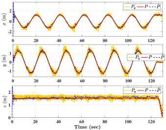
Figure 2: Evolution trajectory of the true vehicle’s position plotted as a red solid line, the estimated position depicted as a blue dash line, and reconstructed position marked as an orange solid line.

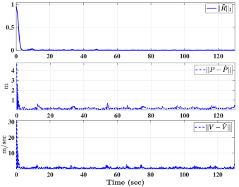
Figure 3: Error convergence of orientation, position, and linear velocity.

VI Conclusion

The inertial navigation problem has been addressed using UWB-IMU fusion to supply measurements to a nonlinear deterministic observer on the Lie Group of $\mathbb{SE}_{2}\left(3\right)$. The observer successfully estimates the vehicle’s orientation, position, and linear velocity ensuring exponential convergence from almost any initial condition. The observer tackles IMU uncertainties and compensates for unknown bias. The proposed observer revealed robust and strong estimation performance when tested using a dataset of measurements collected during a dataset of drone flight and benchmarked against the ground truth.

References

• [1] J. e. a. Li, “Openstreetmap-based autonomous navigation for the four wheel-legged robot via 3d-lidar and ccd camera,” IEEE Transactions on Industrial Electronics, vol. 69, no. 3, pp. 2708–2717, 2021.
• [2] H. A. Hashim, M. Abouheaf, and M. A. Abido, “Geometric stochastic filter with guaranteed performance for autonomous navigation based on IMU and feature sensor fusion,” Control Engineering Practice, vol. 116, p. 104926, 2021.
• [3] C. Zhai, M. Wang, Y. Yang, and K. Shen, “Robust vision-aided inertial navigation system for protection against ego-motion uncertainty of unmanned ground vehicle,” IEEE Transactions on Industrial Electronics, vol. 68, no. 12, pp. 12 462–12 471, 2020.
• [4] D. Zou and et al, “Structvio: visual-inertial odometry with structural regularity of man-made environments,” IEEE Transactions on Robotics, vol. 35, no. 4, pp. 999–1013, 2019.
• [5] H. A. Hashim, “Gps-denied navigation: Attitude, position, linear velocity, and gravity estimation with nonlinear stochastic observer,” in 2021 American Control Conference (ACC).   IEEE, 2021, pp. 1146–1151.
• [6] A. Fornasier, Y. Ng, R. Mahony, and S. Weiss, “Equivariant filter design for inertial navigation systems with input measurement biases,” 2022 IEEE International Conference on Robotics and Automation (ICRA), 2022.
• [7] X. Yang, J. Wang, D. Song, B. Feng, and H. Ye, “A novel nlos error compensation method based imu for uwb indoor positioning system,” IEEE Sensors Journal, vol. 21, no. 9, pp. 11 203–11 212, 2021.
• [8] S. Zihajehzadeh and et al, “Uwb-aided inertial motion capture for lower body 3-d dynamic activity and trajectory tracking,” IEEE Transactions on Instrumentation and Measurement, vol. 64, no. 12, pp. 3577–3587, 2015.
• [9] W. You, F. Li, L. Liao, and M. Huang, “Data fusion of uwb and imu based on unscented kalman filter for indoor localization of quadrotor uav,” IEEE Access, vol. 8, pp. 64 971–64 981, 2020.
• [10] W. Wang, D. Marelli, and M. Fu, “Multiple-vehicle localization using maximum likelihood kalman filtering and ultra-wideband signals,” IEEE Sensors Journal, vol. 21, no. 4, pp. 4949–4956, 2021.
• [11] S. Bottigliero and et al, “A low-cost indoor real-time locating system based on tdoa estimation of uwb pulse sequences,” IEEE Transactions on Instrumentation and Measurement, vol. 70, pp. 1–11, 2021.
• [12] Q. Tian, I. Kevin, K. Wang, and Z. Salcic, “A resetting approach for ins and uwb sensor fusion using particle filter for pedestrian tracking,” IEEE Transactions on Instrumentation and Measurement, vol. 69, no. 8, pp. 5914–5921, 2020.
• [13] G. Kallianpur, Stochastic filtering theory.   Springer Science, 2013.
• [14] E. J. Lefferts, F. L. Markley, and M. D. Shuster, “Kalman filtering for spacecraft attitude estimation,” Journal of Guidance, Control, and Dynamics, vol. 5, no. 5, pp. 417–429, 1982.
• [15] W. Zhao, A. Goudar, X. Qiao, and A. P. Schoellig, “Util: An ultra-wideband time-difference-of-arrival indoor localization dataset,” in International Journal of Robotics Research (IJRR), 2022.
• [16] H. A. Hashim, L. J. Brown, and K. McIsaac, “Nonlinear stochastic attitude filters on the special orthogonal group 3: Ito and stratonovich,” IEEE Transactions on Systems, Man, and Cybernetics: Systems, vol. 49, no. 9, pp. 1853–1865, 2019.
• [17] H. A. Hashim, “Systematic convergence of nonlinear stochastic estimators on the special orthogonal group SO(3),” International Journal of Robust and Nonlinear Control, vol. 30, no. 10, pp. 3848–3870, 2020.
• [18] A. Barrau and S. Bonnabel, “The invariant extended kalman filter as a stable observer,” IEEE Transactions on Automatic Control, vol. 62, no. 4, pp. 1797–1812, 2016.
• [19] H. A. Hashim and F. L. Lewis, “Nonlinear stochastic estimators on the special euclidean group SE(3) using uncertain imu and vision measurements,” IEEE Transactions on Systems, Man, and Cybernetics: Systems, vol. 51, no. 12, pp. 7587–7600, 2021.
• [20] D. Kang, C. Jang, and F. C. Park, “Unscented kalman filtering for simultaneous estimation of attitude and gyroscope bias,” IEEE/ASME Transactions on Mechatronics, vol. 24, no. 1, pp. 350–360, 2019.
• [21] B. N. Stovner, T. A. Johansen, T. I. Fossen, and I. Schjolberg, “Attitude estimation by multiplicative exogenous kalman filter,” Automatica, vol. 95, pp. 347–355, 2018.
• [22] P. S. Maybeck, Stochastic models, estimation, and control.   Academic press, 1982.