On the Degrees of Freedom and Eigenfunctions of Line-of-Sight Holographic MIMO Communications

Abstract

We consider a line-of-sight communication link between two holographic surfaces (HoloSs). We provide a closed-form expression for the number of effective degrees of freedom (eDoF), i.e., the number of orthogonal communication modes that can be established between the HoloSs. The framework can be applied to general network deployments beyond the widely studied paraxial setting. This is obtained by utilizing a quartic approximation for the wavefront of the electromagnetic waves, and by proving that the number of eDoF corresponds to an instance of Landau’s eigenvalue problem applied to a bandlimited kernel determined by the quartic approximation of the wavefront. The proposed approach overcomes the limitations of the widely utilized parabolic approximation for the wavefront, which provides inaccurate estimates in non-paraxial deployments. We specialize the framework to typical network deployments, and provide analytical expressions for the optimal, according to Kolmogorov’s $N$-width criterion, basis functions (communication waveforms) for optimal data encoding and decoding. With the aid of numerical analysis, we validate the accuracy of the closed-form expressions for the number of eDoF and waveforms.

I Introduction

Holographic multiple-input multiple-output (MIMO) is an emerging technology [1], [2]. The reference setup consists of two holographic surfaces (HoloSs) communicating with each other, with a HoloS being an electrically large antenna that is made of a virtually infinite number of radiating elements coupled with electronic circuits and a limited number of radio frequency chains [3]. From a theoretical standpoint, the transmitting HoloS is capable of synthesizing any surface current density fulfilling Maxwell’s equations, and, hence, any radiated electromagnetic field, and the receiving HoloS is capable of sensing any impinging electromagnetic field [4].

From a communication perspective, similar to conventional spatial multiplexing MIMO [5], the theoretical characterization of the performance of a holographic MIMO link consists of identifying the so-called communication modes [6]. A communication mode is defined as a spatial channel through which data can be transmitted in an interference-free manner. The number of interference-free (or orthogonal) spatial channels is referred to as the degrees of freedom (DoF). Generally speaking, the number of DoF may be infinite, but the finite size of the HoloSs and the finite spatial bandwidth of the transmission channel result in a finite number of strongly connected communication channels, where strongly connected refers to a spatial channel that carries a good portion of the total system (transmit) power. The number of strongly connected communication channels is referred to as the number of effective DoF (eDoF). A rigorous definition of eDoF originates from approximation theory in general multi-dimensional Hilbert spaces: The number of eDoF coincides with the minimum value of $N$ for which Kolmogorov’s $N$-width is less than a predefined level of accuracy [7]. In simple terms, the number of eDoF is the minimum number of optimal basis functions that is needed to represent any surface current density at the transmitting HoloS and any received electromagnetic field at the receiving HoloS within a certain maximum error [8]. Specifically, a set of $N$ basis functions is referred to as optimal if, among all the possible choices of $N$ orthonormal functions, it minimizes the approximation error for a given $N$. The optimal basis functions for the transmitting and receiving HoloSs are usually different but are not independent. Interested readers are referred to [9], [10] and to the textbooks in [7] and [8] for a comprehensive overview and an historical perspective on the number of eDoF and Kolmogorov’s $N$-width in approximation theory.

The theoretical characterization of the performance of a holographic MIMO link reduces, therefore, to the computation of the number of eDoF and the optimal basis functions to represent any surface current density and received electromagnetic field at the transmitting and receiving HoloSs, respectively [11]. This is the main focus of the present paper. In this context, the most related prior art includes [12, 13, 14, 15, 10]. In [12], the author has introduced a general framework for estimating the eDoF and the optimal basis functions as the solution of two eigenproblems. The approach is applicable to scalar electromagnetic fields in free-space, and leverages the theory of compact and self-adjoint operators over Hilbert spaces [16]. Under the assumption of a parabolic approximation for the wavefront of the electromagnetic waves and assuming a paraxial setup, the author shows that the optimal basis functions are related to the prolate spheroidal wave functions (PSWFs), and the number of eDoF immediately follows from the energy concentration property of the PSWFs. The approach is generalized in [13] for application to vector electromagnetic fields and for propagation over general channels (beyond the free space scenario). The approach in [12] and [13] is general, but, with the exception of the paraxial setup, requires extensive numerical computations, and the number of eDoF and the optimal basis functions can only be determined numerically. To overcome these limitations, the author of [14] provides an approximate approach to compute the number of eDOF based on the computation of an integral obtained from the wavevector between the transmitting and receiving HoloSs. Computationally, the approach is simpler than the solution of the eigenproblem in [12] and [13]. Also, the author of [14] provides a closed-form expression for the number of eDOF when one of the two HoloSs is sufficiently small compared with the distance, and the two HoloSs are either parallel or orthogonal to one another. In the general case, however, the approach is still numerical and the optimal communication functions are not discussed. To fill these gaps, the authors of [15] depart from [14], and introduce approximated basis functions based on the concept of focusing functions. The orthonormal functions are constructed iteratively, and, based on geometric considerations, an approximate expression for the number eDoF is given when one of the HoloS is small enough compared to the distance between the HoloSs. The approach is applicable to lines, and leads to an approximate design. More recently, the authors of [10] have established a connection between the number of eDoF of the eigenproblem formulated in [12] for scalar electromagnetic fields and Landau’s eigenvalue problem [17]. Under the paraxial approximation, more precisely, the two problems are shown to be equivalent, and, therefore, the authors provide estimates of the number of eDoF for some channel models. The approach is, however, applicable only under the paraxial approximation and no discussion about the optimal basis functions is given. The frameworks in [10] and [12] are based on a parabolic approximation for the wavefront of the electromagnetic waves. As recently remarked in [18], the parabolic approximation is typically sufficiently accurate under the paraxial setup, but its accuracy in general deployments cannot be anticipated. Finally, the authors of [19] offer a numerical study of the number of eDoF, and confirm the limitations of the paraxial approximation for application to general deployments.

Motivated by these consideration, we introduce an analytical framework for estimating the number of eDoF of holographic MIMO beyond the paraxial setup, and provide closed-form expressions for the optimal communication waveforms for typical network deployments. To focus on the key aspects of the approach, the framework is elaborated for line-of-sight channels, which are receiving major attention from the research community especially in the context of (sub-)terahertz communications [20], [21]. The generalization in the presence of scattering objects is postponed to future research.

The contributions made by this paper are as follows:

• We depart from the eigenproblem formulated in [12] involving compact and self-adjoint operators, and provide a closed-form expression for the number of eDoF in non-paraxial setups. We propose a quartic approximation for the wavefront of the electromagnetic waves, and, in agreement with [18], we prove the inaccuracy of the widely used parabolic approximation for the wavefront when applied to non-paraxial setups. The number of eDoF is obtained by establishing an equivalence between Landau’s eigenvalue theorem and the kernel of the eigenproblem based on the proposed quartic approximation.

• The number of eDoF is obtained in two steps: (i) we obtain a closed-form formulation in the radiative near-field when the size of the HoloSs is not too large, so that the transmission distance between two arbitrary points of the HoloSs is well approximated by their center-point distance; and (ii) we generalize the approach by integrating the obtained number of eDoF over the actual transmission distance between any two points of the HoloSs. The approach has general applicability. By specializing it to the case studies in [14], we retrieve the same results.

• The proposed analytical framework can be applied to arbitrary network deployments, which include arbitrary tilts and rotations of the HoloSs. We prove that there exist optimal values of the angles of tilt and rotation that maximize the number of eDoF, and we provide closed-form expressions for the equations that they fulfill.

• We specialize the considered eigenproblem based on the quartic approximation for the wavefront to network deployments, beyond the paraxial setting, typically encountered in communications. In these scenarios, we provide closed-form expressions for the optimal communication waveforms, which are shown to be related to PSWFs.

• The analytical findings are validated by numerically solving the exact formulation of the considered eigenproblem.

The remainder of the present paper is organized as follows. In Sec. II, we provide mathematical preliminaries on compact, self-adjoint operators and Kolmogorov’s $N$-widths. In Sec. III, we introduce the system model and problem formulation. In Sec. IV, we summarize the proposed approach. In Sec. V, we provide the analytical framework to compute the number of eDoF. In Sec. VI, we analyze relevant network settings, and identify the optimal communication waveforms. In Sec. VII, we illustrate numerical results to validate the proposed approach, and the quartic in lieu of the parabolic approximation for the wavefront. Conclusions are drawn in Sec. VIII.

Notation: Bold lower and upper case letters represent vectors and matrices. Calligraphic letters denote sets. $(\cdot)$ is the scalar product. $(\cdot)^{*}$ is the conjugate transpose operator. $m(\mathcal{S})$ is the Lebesgue measure of $\mathcal{S}$. $j=\sqrt{-1}$ is the imaginary unit. $\left\langle{f\left({\bf{x}}\right),g\left({\bf{x}}\right)}\right\rangle=\int{f\left({\bf{x}}\right){g^{*}}\left({\bf{x}}\right)d{\bf{x}}}$ is the inner product of the functions ${f\left({\bf{x}}\right)}$ and ${g\left({\bf{x}}\right)}$. $\left|{\cdot}\right|$ is the ${\ell}^{2}$-norm of a vector. $\nabla=\left[\frac{\partial}{\partial x},\frac{\partial}{\partial y},\frac{\partial}{\partial z}\right]$ is the gradient operator. $\operatorname{sinc}(x)=\sin(\pi x)/(\pi x)$ is the sinc function. $\operatorname{rect}{(x)}$ is the boxcar function that is equal to one if $x\in(-1/2,1/2)$ and is zero elsewhere. $\det\mathbf{(A)}$ is the determinant of the matrix $\mathbf{A}$. $\mathds{1}_{\mathcal{P}}(\mathbf{x})$ is the indicator function over the set ${\mathcal{P}}$, i.e., $\mathds{1}_{\mathcal{P}}(\mathbf{x})=1$ if $\mathbf{x}\in\mathcal{P}$ and zero otherwise.

II Mathematical Preliminaries

In this section, we summarize definitions and results from the mathematical literature, which are utilized in the rest of the paper. Specifically, this includes: (i) theory and results (notably the spectral theorem) pertaining to compact and self-adjoint operators over $n$-dimensional spaces; (ii) Kolmogorov’s $n$-widths in approximation theory over $n$-dimensional spaces; and (iii) Landau’s eigenvalue theorem over $n$-dimensional spaces for a class of compact and self-adjoint operators.

Definition 1. Let $\mathbb{L}^{2}(\mathcal{S})$ be the Hilbert space of square-integrable complex-valued functions defined on the set $\mathcal{S}\subset\mathbb{R}^{n}$, where $\mathbb{R}^{n}$ is the $n$-dimensional real space. An operator $K:\mathbb{L}^{2}(\mathcal{S}_{i})\to\mathbb{L}^{2}(\mathcal{S}_{o})$ with kernel ${k\left({{\bf{x}},{\bf{y}}}\right)}$ for ${{\bf{x}}}\in\mathcal{S}_{i}$ and ${{\bf{y}}}\in\mathcal{S}_{o}$ applied to the function $\phi\left({\bf{x}}\right)\in\mathbb{L}^{2}(\mathcal{S}_{i})$ is defined as $\psi\left({\bf{y}}\right)=\left({K\phi}\right)\left({\bf{y}}\right)=\int_{\mathcal{S}_{i}}{k\left({{\bf{x}},{\bf{y}}}\right)\phi\left({\bf{x}}\right)d{\bf{x}}}\in\mathbb{L}^{2}(\mathcal{S}_{o})$ [16].

Definition 2. Consider the operator $K$ in Def. 1. Assume that the kernel ${k\left({{\bf{x}},{\bf{y}}}\right)}$ fulfills $K^{\rm{norm}}=\int_{{{\mathcal{S}}_{i}}}{\int_{{{\mathcal{S}}_{o}}}{{{\left|{k\left({{\bf{x}},{\bf{y}}}\right)}\right|}^{2}}d{\bf{x}}d{\bf{y}}}}<\infty$, i.e., the kernel is a sufficiently well-behaved function. Then, the operator $K$ is bounded and compact [16, Sec. 3.4]. If $K^{\rm{norm}}\leq 1$, the operator $K$ is said to be bounded by one.

Definition 3. Consider the compact operator $K$ in Def. 2. A complex-valued scalar $\mu$ is an eigenvalue of $K$ if there exists a complex-valued function $\phi\left({\bf{x}}\right)\in\mathbb{L}^{2}(\mathcal{S}_{i})$ such that $\left({K\phi}\right)\left({\bf{x}}\right)=\mu\phi\left({\bf{x}}\right)$. $\phi\left({\bf{x}}\right)$ is termed eigenfunction [16, Def. 4.1].

Lemma 1. Consider the compact operator $K$ in Def. 2. Let $\left\{{{\mu_{m}}}\right\}$ be a (possibly infinite) sequence of distinct eigenvalues of $K$ as per Def. 3. Let $\left\{{{\mu_{m}}}\right\}$ be ordered with non-increasing magnitude. Then, ${\mu_{m}}\to 0$ as $m\to\infty$ [16, Th. 4.6].

Definition 4. Consider the compact operator $K:\mathbb{L}^{2}(\mathcal{S}_{i})\to\mathbb{L}^{2}(\mathcal{S}_{o})$ in Def. 2. The adjoint of $K$ is the compact operator $K_{a}:\mathbb{L}^{2}(\mathcal{S}_{o})\to\mathbb{L}^{2}(\mathcal{S}_{i})$ that fulfills the property $\left\langle{\left({K\phi}\right)\left({\bf{x}}\right),\psi\left({\bf{x}}\right)}\right\rangle=\left\langle{\phi\left({\bf{x}}\right),\left({{K_{a}}\psi}\right)\left({\bf{x}}\right)}\right\rangle$ [16, Def. 4.2]. By definition, the kernel, ${k_{a}\left({{\bf{x}},{\bf{y}}}\right)}$, of $K_{a}$ is the complex conjugate of the kernel, ${k\left({{\bf{x}},{\bf{y}}}\right)}$, of $K$, i.e., ${k_{a}\left({{\bf{x}},{\bf{y}}}\right)}={k^{*}\left({{\bf{x}},{\bf{y}}}\right)}$.

Definition 5. Consider the compact operator $K:\mathbb{L}^{2}(\mathcal{S})\to\mathbb{L}^{2}(\mathcal{S})$ and its adjoint $K_{a}:\mathbb{L}^{2}(\mathcal{S})\to\mathbb{L}^{2}(\mathcal{S})$ in Def. 4. If $K=K_{a}$, $K$ is termed self-adjoint. Under the considered assumptions, $K$ is self-adjoint if and only if ${k\left({{\bf{x}},{\bf{y}}}\right)}$ coincides with its complex conjugate, i.e., ${k\left({{\bf{x}},{\bf{y}}}\right)}={k^{*}\left({{\bf{x}},{\bf{y}}}\right)}={k_{a}\left({{\bf{x}},{\bf{y}}}\right)}$ [16, Sec. 4.4].

Lemma 2. Let $K:\mathbb{L}^{2}(\mathcal{S})\to\mathbb{L}^{2}(\mathcal{S})$ be the self-adjoint operator in Def. 5. The eigenvalues of $K$ are real and the eigenvectors of distinct eigenvalues are orthogonal [16, Lemma 4.12].

Lemma 3 (spectral theorem). Let $K:\mathbb{L}^{2}(\mathcal{S})\to\mathbb{L}^{2}(\mathcal{S})$ be a self-adjoint operator according to Def. 5. Then, there exists a, possibly finite, sequence $\left\{{{\mu_{m}}}\right\}$ of real and non-zero eigenvalues of $K$ and a corresponding orthonormal sequence $\left\{{{\phi_{m}}}\left({\bf{x}}\right)\right\}$ of eigenvectors, such that, for each $\phi\left({\bf{x}}\right)\in\mathbb{L}^{2}(\mathcal{S})$, $\left({K\phi}\right)\left({\bf{x}}\right)=\sum\nolimits_{m=1}^{\infty}{{\mu_{m}}\left\langle{\phi\left({\bf{x}}\right),{\phi_{m}}\left({\bf{x}}\right)}\right\rangle{\phi_{m}}\left({\bf{x}}\right)}$, with the sum being finite if the number of eigenvalues is finite. Consider the operator $\left({K_{N}\phi}\right)\left({\bf{x}}\right)=\sum\nolimits_{m=1}^{N}{{\mu_{n}}\left\langle{\phi\left({\bf{x}}\right),{\phi_{m}}\left({\bf{x}}\right)}\right\rangle{\phi_{m}}\left({\bf{x}}\right)}:\mathbb{L}^{2}(\mathcal{S})\to\mathbb{L}^{2}(\mathcal{S})$. If the eigenvalues are infinitely many, then $\left\|{\left({K\phi}\right)\left({\bf{x}}\right)-\left({{K_{N}}\phi}\right)\left({\bf{x}}\right)}\right\|\to 0$ as $N\to\infty$ [16, Th. 4.15].

Lemma 4. Let $K:\mathbb{L}^{2}(\mathcal{S})\to\mathbb{L}^{2}(\mathcal{S})$ and $\left\{{{\phi_{n}}}\left({\bf{x}}\right)\right\}$ be the operator and the eigenfunctions in Lemma 3. For any $\phi\left({\bf{x}}\right)\in\mathbb{L}^{2}(\mathcal{S})$, there exists a $\phi_{0}\left({\bf{x}}\right)\in\mathbb{L}^{2}(\mathcal{S})$ so that $\phi\left({\bf{x}}\right)={\phi_{0}}\left({\bf{x}}\right)+$ $\sum\nolimits_{m=1}^{\infty}{\left\langle{\phi\left({\bf{x}}\right),{\phi_{m}}\left({\bf{x}}\right)}\right\rangle{\phi_{m}}\left({\bf{x}}\right)}$ and $\left({K{\phi_{0}}}\right)\left({\bf{x}}\right)=0$ [16, Cor. 4.16].

Lemma 5. Let $K:\mathbb{L}^{2}(\mathcal{S})\to\mathbb{L}^{2}(\mathcal{S})$ and $\left\{{{\phi_{m}}}\left({\bf{x}}\right)\right\}$ be the operator and the eigenfunctions in Lemma 3. Then, $\left\{{{\phi_{m}}}\left({\bf{x}}\right)\right\}$ is a complete orthonormal basis in $\mathbb{L}^{2}(\mathcal{S})$ [16, Cor. 4.17].

Based on the definitions and lemmas summarized from [16], we evince that the eigenfunctions of a compact and self-adjoint operator constitute a complete orthonormal basis. Thus, any function can be expressed as a (possibly infinite) linear combination of these eigenfunctions. Two important aspects remain, however, open: (i) the optimality of the eigenfunctions in terms of approximation accuracy provided by the truncated operator $K_{N}$ in Lemma 3 (given $N$); and (ii) the evaluation of the effective number, $N_{\rm{eDoF}}$, of eigenfunctions providing a non-negligible contribution. $N_{\rm{eDoF}}$ is referred to as the number of eDoF introduced in Sec. I [7]. This is elaborated next.

Definition 6. Consider the compact operator $K:\mathbb{L}^{2}(\mathcal{S}_{i})$ $\to\mathbb{L}^{2}(\mathcal{S}_{o})$ in Def. 2 and denote $\text{X}_{o}=\mathbb{L}^{2}(\mathcal{S}_{o})$. Let $\text{X}_{k}\subset\text{X}_{o}$ be the subspace of functions ${\psi_{k}\left({\bf{y}}\right)}=\left({K\phi}\right)\left({\bf{y}}\right)$ determined by the kernel $K$ for ${\phi\left({\bf{x}}\right)}\in\mathbb{L}^{2}(\mathcal{S}_{i})$. The Kolmogorov $N$-width of $\text{X}_{k}$ in $\text{X}_{o}$ is defined as ${d_{N}}\left({{{\rm{X}}_{k}};{{\rm{X}}_{o}}}\right)={\inf_{{{\rm{X}}_{o,N}}\subset{{\rm{X}}_{o}}}}$ ${\sup_{{}_{{\psi_{k}}\left({\bf{y}}\right)\in{{\rm{X}}_{k}}}}}{\inf_{{\psi_{o,N}}\left({\bf{y}}\right)\in{{\rm{X}}_{o,n}}}}\left\|{{\psi_{k}}\left({\bf{y}}\right)-{\psi_{o,N}}\left({\bf{y}}\right)}\right\|$, where ${{{\rm{X}}_{o,N}}}$ is an $N$-dimensional subspace of ${{{\rm{X}}_{o}}}$ [7, Ch. 2, Def. 1.1]. Thus, ${D_{{{\rm{X}}_{o,N}}}}\left({{{\rm{X}}_{k}}}\right)={\sup_{{}_{{\psi_{k}}\left({\bf{y}}\right)\in{{\rm{X}}_{k}}}}}{\inf_{{\psi_{o,N}}\left({\bf{y}}\right)\in{{\rm{X}}_{o,N}}}}\left\|{{\psi_{k}}\left({\bf{y}}\right)-{\psi_{o,N}}\left({\bf{y}}\right)}\right\|$ is a measure of how well the worst function in ${{{\rm{X}}_{k}}}$ is approximated by ${{{\rm{X}}_{o,N}}}$. ${d_{N}}\left({{{\rm{X}}_{k}};{{\rm{X}}_{o}}}\right)$ is the smallest ${D_{{{\rm{X}}_{o,N}}}}\left({{{\rm{X}}_{k}}}\right)$ over all possible $N$-dimensional subspaces ${{{\rm{X}}_{o,N}}}\subset{{{\rm{X}}_{o}}}$.

Lemma 6. Consider the compact operator $K:\mathbb{L}^{2}(\mathcal{S}_{i})\to\mathbb{L}^{2}(\mathcal{S}_{o})$ in Def. 2 and its adjoint $K_{a}:\mathbb{L}^{2}(\mathcal{S}_{o})\to\mathbb{L}^{2}(\mathcal{S}_{i})$ in Def. 4. Define the operators $K_{i}=KK_{a}:\mathbb{L}^{2}(\mathcal{S}_{i})\to\mathbb{L}^{2}(\mathcal{S}_{i})$ and $K_{o}=K_{a}K:\mathbb{L}^{2}(\mathcal{S}_{o})\to\mathbb{L}^{2}(\mathcal{S}_{o})$ whose kernels are ${k_{i}}\left({{{\bf{x}}_{1}},{{\bf{x}}_{2}}}\right)=\int\nolimits_{{{\mathcal{S}}_{o}}}{k\left({{{\bf{x}}_{1}},{\bf{y}}}\right){k^{*}}\left({{{\bf{x}}_{2}},{\bf{y}}}\right)d{\bf{y}}}$ and ${k_{o}}\left({{{\bf{y}}_{1}},{{\bf{y}}_{2}}}\right)=\int\nolimits_{{{\mathcal{S}}_{i}}}{k\left({{\bf{x}},{{\bf{y}}_{1}}}\right){k^{*}}\left({{\bf{x}},{{\bf{y}}_{2}}}\right)d{\bf{x}}}$, respectively. The operators $K_{i}$ and $K_{o}$ are compact, self-adjoint, and non-negative, i.e., their eigenvalues are non-negative [7, Ch. 4, pg. 65].

Definition 7. Consider the compact operator $K$ and the compact, self-adjoint, non-negative operator $K_{o}$ in Lemma 6. The s-values of $K$ are defined as ${s_{m}}\left(K\right)=\sqrt{{\mu_{m}}\left({{K_{o}}}\right)}$ for $m=1,2,\ldots$, with $\mu_{m}$ being the eigenvalues of $K_{o}$ [7, pg. 65].

Lemma 7. Consider the compact operators $K$, its adjoint $K_{a}$, and the compact, self-adjoint, and non-negative operators $K_{i}$ and $K_{o}$ in Lemma 6. Let $\left\{{{\mu_{m}}}\right\}$ and $\left\{{{\phi_{m}}}\left({\bf{x}}\right)\right\}$ be the sequence of non-zero and positive eigenvalues and orthonormal eigenvectors of $K_{o}$, respectively. Then, ${d_{N}}\left({{{\rm{X}}_{k}};{{\rm{X}}_{o}}}\right)={s_{N+1}}\left(K\right)$, the functions $\left\{{{\phi_{m}}}\left({\bf{x}}\right)\right\}$ constitute a complete orthonormal basis in ${{\rm{X}}_{o,N}}$, and the subspace ${{\rm{X}}_{o,N}}$ constituted by all possible linear combinations of $\left\{{{\phi_{m}}}\left({\bf{x}}\right)\right\}$, i.e., ${{\rm{X}}_{o,N}}={\rm{span}}\left\{{{\phi_{1}}\left({\bf{x}}\right),{\phi_{2}}\left({\bf{x}}\right),\ldots,{\phi_{N}}\left({\bf{x}}\right)}\right\}$ minimizes the Kolmogorov $N$-width ${d_{N}}\left({{{\rm{X}}_{k}};{{\rm{X}}_{o}}}\right)$ [7, Ch. 4, Th. 2.2]. In simple terms, given a compact and self-adjoint operator $K$ from an input space to an output space and its adjoint $K_{a}$, the optimal basis functions, in terms of approximation accuracy according to Kolmogorov’s definition, coincide with the eigenfunctions of the compact, self-adjoint, and non-negative operator given by $K_{a}K$ for the output space (and by $KK_{a}$ for the input space). Also, the approximation error by considering $N$ basis functions coincides with the square root of the $(N+1)$th eigenvalue of $K_{a}K$ for the output space (and of $KK_{a}$ for the input space).

Definition 8. Consider the compact operator $K$ and the compact, self-adjoint, and non-negative operator $K_{o}$ in Lemma 6. The number of degrees of freedom is the minimum dimension of the approximating subspace such that the Kolmogorov $N$-width is no greater than $\gamma$ with $0<\gamma<1$, i.e., the level of approximation accuracy is $\gamma$. By using the notation in Def. 6, it holds ${{{N}}_{{\rm{eDoF}}}}\left(\gamma\right)=\min\left\{{N:{d_{N}^{2}}\left({{{\rm{X}}_{k}};{{\rm{X}}_{o}}}\right)\leq\gamma}\right\}$ [8].

Lemma 8. Consider a function $f\left({\bf{x}}\right)$ in the Hilbert space of square-integrable complex-valued functions, and its Fourier transform $F\left({\boldsymbol{\nu}}\right)=\left({Tf}\right)\left({\boldsymbol{\nu}}\right)$, where $T$ is the Fourier transform operator. Consider the operators $\left({{D_{\mathcal{U}}}f}\right)\left({\bf{x}}\right)={{\mathds{1}}_{\mathcal{U}}}\left({\bf{x}}\right)f\left({\bf{x}}\right)$, $\left({{B_{\mathcal{S}}}f}\right)\left({\bf{x}}\right)=\int{{h_{\mathcal{S}}}\left({{\bf{x}}-{\bf{y}}}\right)f\left({\bf{y}}\right)d{\bf{y}}}$, and $\left({T{h_{\mathcal{S}}}}\right)\left({{\boldsymbol{\nu}}}\right)={{\mathds{1}}_{\mathcal{S}}}\left({{\boldsymbol{\nu}}}\right)$, where $\mathcal{U}$ and $\mathcal{S}$ are sets in $\mathbb{R}^{n}$, and ${h_{\mathcal{S}}}\left({\bf{x}}\right)$ is a kernel whose Fourier transform is an ideal filter in ${\mathcal{S}}$, i.e., its Fourier transform is one if ${\bf{\nu}}\in{\mathcal{S}}$ and is zero elsewhere. Assume that ${\mathcal{S}}$ is fixed and let ${\mathcal{U}}$ vary over the family $r{\mathcal{Q}}$ with ${\mathcal{Q}}$ being fixed. Consider the operator ${D_{r{\mathcal{Q}}}}{B_{\mathcal{S}}}{D_{r{\mathcal{Q}}}}$, and assume that it is bounded by one, according to Def. 2. Let ${N_{r}}\left(\gamma\right)$ be the number of eigenvalues of ${D_{r{\mathcal{Q}}}}{B_{\mathcal{S}}}{D_{r{\mathcal{Q}}}}$ that are no smaller than $0<\gamma<1$. Then, ${\lim_{r\to\infty}}{r^{-n}}{N_{r}}\left(\gamma\right)={\left({2\pi}\right)^{-n}}m\left({\mathcal{Q}}\right)m\left({\mathcal{S}}\right)$ $={{{N}}_{{\rm{eDoF}}}}$ [17, Th. 1]. In simple terms, the eigenvalues of ${D_{r{\mathcal{Q}}}}{B_{\mathcal{S}}}{D_{r{\mathcal{Q}}}}$ polarize asymptotically so that the number of leading, i.e., nearly equal to one, eigenvalues is ${{{N}}_{{\rm{eDoF}}}}$ and the others are nearly equal to zero. In one-dimensional spaces, the transition band between the leading (nearly one) and the nearly zero eigenvalues is known [8, Eq. (2.132)], [17].

Remark 1. Lemma 8 requires that the operator $K_{BD}={D_{r{\mathcal{Q}}}}{B_{\mathcal{S}}}{D_{r{\mathcal{Q}}}}$ is bounded by one, i.e., $K_{BD}^{\rm{norm}}\leq 1$, according to Def. 2 (besides being compact, non-negative, and self-adjoint). This implies that every eigenvalue of $K_{BD}$ has modulus at most equal to $K_{BD}^{\rm{norm}}\leq 1$ [16, Proof of Th. 4.7]. If the operator $K_{BD}$ is bounded but not necessarily by one, i.e., $K_{BD}^{\rm{norm}}\leq K_{BD}^{\rm{bound}}$, with $K_{BD}^{\rm{bound}}>1$ but finite, Lemma 8 can be applied to the normalized operator $K_{BD}/K_{BD}^{\rm{bound}}$. Alternatively, Lemma 8 can be directly applied to the eigenvalues of $K_{BD}$, by first normalizing them by the largest eigenvalue of $K_{BD}$.

III Problem Formulation

We consider a transmitting and a receiving HoloSs located at $\mathbf{r}_{Tx}=\left(x_{Tx},y_{Tx},z_{Tx}\right)\in\mathcal{S}_{Tx}$ and $\mathbf{r}_{Rx}=\left(x_{Rx},y_{Rx},z_{Rx}\right)\in\mathcal{S}_{Rx}$, with surface areas $A_{Tx}=m(\mathcal{S}_{Tx})$ and $A_{Rx}=m(\mathcal{S}_{Rx})$. The surface current density at $\mathbf{r}_{Tx}\in\mathcal{S}_{T}$ is denoted by $\mathbf{J}(\mathbf{r}_{Tx})$. We assume the transmission of a monochromatic electromagnetic wave at frequency $f_{0}$. By Maxwell’s equations, the electric field observed at $\mathbf{r}_{Rx}\in\mathcal{S}_{Rx}$ is [13, Eq. (3.3)]

$$\mathbf{E}(\mathbf{r}_{Rx})=\int_{\mathcal{S}_{Tx}}\bar{\bar{\mathbf{G}}}(\mathbf{r}_{Rx}-\mathbf{r}_{Tx})\mathbf{J}(\mathbf{r}_{Tx})d\mathbf{r}_{Tx}$$ (1)

where $\bar{\bar{\mathbf{G}}}(\mathbf{r}_{Rx}-\mathbf{r}_{Tx})$ is the dyadic Green function.

Equation (1) can be applied to any linear, in general shift-variant, system. Specifically, it can be applied for modeling the propagation of electromagnetic waves between transmitting and receiving domains in the presence of material bodies, e.g., blocking obstacles or scattering surfaces [13]. To highlight the key aspects of the proposed approach, we focus our attention on the free space scenario, which is receiving major renewed attention lately [20], [21]. In free space, the dyadic Green function $\bar{\bar{\mathbf{G}}}(\mathbf{r})$ can be expressed as [22, Eq. 1.3.49]

$$\bar{\bar{\mathbf{G}}}(\mathbf{r})=\frac{j\omega_{0}\mu}{4\pi}\left(\bar{\bar{{\mathbf{I}}}}+\frac{1}{k_{0}^{2}}\nabla\nabla\right)\frac{\exp(-jk_{0}|\mathbf{r}|)}{|\mathbf{r}|}$$ (2)

where $\mathbf{r}=\mathbf{r}_{Rx}-\mathbf{r}_{Tx}$, $k_{0}=2\pi/\lambda$ is the wavenumber, $\lambda=c/f_{0}$ is the wavelength, $\omega_{0}=2\pi f_{0}$ is the angular frequency, $\mu$ is the magnetic permeability, and $\bar{\bar{{\bf I}}}=\hat{\mathbf{u}}_{x}\hat{\mathbf{u}}_{x}^{*}+\hat{\mathbf{u}}_{y}\hat{\mathbf{u}}_{y}^{*}+\hat{\mathbf{u}}_{z}\hat{\mathbf{u}}_{z}^{*}$ is the identity dyadic tensor with $\hat{\mathbf{u}}_{a}$ denoting the unit-norm vector in the direction of the $a$-axis for $a=\left\{{x,y,z}\right\}$.

Usually, wireless communication systems do not operate in the reactive near-field, and we can assume $|\mathbf{r}|\gg\lambda$ [3]. Under this assumption, $\bar{\bar{{\mathbf{G}}}}$ can be approximated as [14, Eq. (3)]

$$\bar{\bar{{\mathbf{G}}}}(\mathbf{r})\approx G(|\mathbf{r}|)\left(\bar{\bar{{\mathbf{I}}}}-\hat{\mathbf{r}}\hat{\mathbf{r}}^{*}\right),\quad G(|\mathbf{r}|)=\frac{j\eta\exp(-jk_{0}|\mathbf{r}|)}{2\lambda|\mathbf{r}|}$$ (3)

where $\hat{\mathbf{r}}=\mathbf{r}/|\mathbf{r}|$ and $\eta=\sqrt{{\mu\mathord{\left/{\vphantom{\mu\varepsilon}}\right.\kern-1.2pt}\varepsilon}}$ with $\varepsilon$ the electric permittivity.

With no loss of generality, we assume that the considered communication system is probed by exciting one polarization of $\mathbf{J}(\mathbf{r}_{Tx})$ at a time. Considering the polarization along the $i$-axis, i.e., $\mathbf{J}(\mathbf{r}_{Tx})=J_{i}(\mathbf{r}_{Tx})\hat{\mathbf{u}}_{i}$ for $i=\left\{{x,y,z}\right\}$, and denoting $\mathbf{r}=x_{TR}\hat{\mathbf{u}}_{x}+y_{TR}\hat{\mathbf{u}}_{y}+z_{TR}\hat{\mathbf{u}}_{z}$ with $a_{TR}=a_{Rx}-a_{Tx}$ for $a=\left\{{x,y,z}\right\}$, the received electric field reduces to

$$\mathbf{E}_{i}(\mathbf{r}_{Rx}) \approx\int_{\mathcal{S}_{Tx}}G(|\mathbf{r}|)\left[\bar{\bar{{\mathbf{I}}}}\hat{\mathbf{u}}_{i}-\frac{\mathbf{r}\left(\mathbf{r}^{*}\hat{\mathbf{u}}_{i}\right)}{|\mathbf{r}|^{2}}\right]J_{i}(\mathbf{r}_{Tx})d\mathbf{r}_{Tx}$$ (4)

$$=\int_{\mathcal{S}_{Tx}}G(|\mathbf{r}|)\left(\hat{\mathbf{u}}_{i}-\frac{i_{TR}}{|\mathbf{r}|^{2}}{\mathbf{r}}\right)J_{i}(\mathbf{r}_{Tx})d\mathbf{r}_{Tx}\,.$$ (5)

Explicitly, the three Cartesian components of $\mathbf{E}_{i}(\mathbf{r}_{Rx})=E_{i,x}(\mathbf{r}_{Rx})\hat{\mathbf{u}}_{x}+E_{i,y}(\mathbf{r}_{Rx})\hat{\mathbf{u}}_{y}+E_{i,z}(\mathbf{r}_{Rx})\hat{\mathbf{u}}_{z}$ can be written as

$$E_{i,o}(\mathbf{r}_{Rx})=\int_{\mathcal{S}_{Tx}}G(|\mathbf{r}|){e_{i,o}}\left({{{\bf{r}}_{Tx}},{{\bf{r}}_{Rx}}}\right)J_{i}(\mathbf{r}_{Tx})d\mathbf{r}_{Tx}$$ (6)

where ${e_{i,o}}\left({{{\bf{r}}_{Tx}},{{\bf{r}}_{Rx}}}\right)={{{\bf{\hat{u}}}}_{i}}\cdot{{{\bf{\hat{u}}}}_{o}}-\left({{i_{TR}}/{{\left|{\bf{r}}\right|}^{2}}}\right){\bf{r}}\cdot{{{\bf{\hat{u}}}}_{o}}$ accounts for the coupling between the $i$th component of the surface current density and the $o$th component of the received electric field.

From Def. 1, we evince that (6) is an operator $G_{i,o}:$ $\mathbb{L}^{2}(\mathcal{S}_{Tx})\to\mathbb{L}^{2}(\mathcal{S}_{Rx})$, whose kernel is $g_{i,o}\left({{{\bf{r}}_{Tx}},{{\bf{r}}_{Rx}}}\right)=G\left({\left|{\bf{r}}\right|}\right){e_{i,o}}\left({{{\bf{r}}_{Tx}},{{\bf{r}}_{Rx}}}\right)$. Based on Def. 2, $G_{i,o}$ is compact, since $\int_{{{\mathcal{S}}_{Tx}}}{\int_{{{\mathcal{S}}_{Rx}}}{{{\left|{g_{i,o}\left({{{\bf{r}}_{Tx}},{{\bf{r}}_{Rx}}}\right)}\right|}^{2}}d{{{\bf{r}}_{Tx}}}d{{{\bf{r}}_{Rx}}}}}<\infty$ by virtue of the radiation boundary conditions. Based on Lemma 7, the number of eDoF and the optimal pair of communication waveforms at the transmitting (encoding) and receiving (decoding) HoloSs are the solutions, respectively, of the eigenproblems

$$\mu_{m}\phi_{m}(\mathbf{r}_{Tx})=\int_{{\mathcal{S}}_{Tx}}G_{Tx}(\mathbf{r}_{Tx},\mathbf{r}_{Tx}^{\prime})\phi_{m}(\mathbf{r}_{Tx}^{\prime})d\mathbf{r}_{Tx}^{\prime}$$ (7)

$$\mu_{m}\psi_{m}(\mathbf{r}_{Rx})=\int_{{\mathcal{S}}_{Rx}}G_{Rx}(\mathbf{r}_{Rx},\mathbf{r}_{Rx}^{\prime})\psi_{m}(\mathbf{r}_{Rx}^{\prime})d\mathbf{r}_{Rx}^{\prime}$$ (8)

where $\mu_{m}$ are the real-valued and positive eigenvalues for $m=1,2,\ldots,{{{N}}_{{\rm{eDoF}}}}\left(\cdot\right)$ according to Def. 8, $\left\{{{\phi_{m}}}\right\}$ and $\left\{{{\psi_{m}}}\right\}$ are the corresponding pair of orthogonal communication waveforms at the transmitting and receiving HoloSs, respectively, and the kernels $G_{Tx}(\mathbf{r}_{Tx},\mathbf{r}_{Tx}^{\prime})$ and $G_{Rx}(\mathbf{r}_{Rx},\mathbf{r}_{Rx}^{\prime})$ are defined as

$$G_{Tx}(\mathbf{r}_{Tx},\mathbf{r}_{Tx}^{\prime})=\int_{{\mathcal{S}}_{Rx}}g_{i,o}^{*}(\mathbf{r}_{Tx},\mathbf{r}_{Rx})g_{i,o}(\mathbf{r}_{Tx}^{\prime},\mathbf{r}_{Rx})d\mathbf{r}_{Rx}$$ (9)

$$G_{Rx}(\mathbf{r}_{Rx},\mathbf{r}_{Rx}^{\prime})=\int_{{\mathcal{S}}_{Tx}}g_{i,o}^{*}(\mathbf{r}_{Tx},\mathbf{r}_{Rx})g_{i,o}(\mathbf{r}_{Tx},\mathbf{r}_{Rx}^{\prime})d\mathbf{r}_{Tx}\,.$$ (10)

Based on Lemma 6, $G_{Tx}(\mathbf{r}_{Tx},\mathbf{r}_{Tx}^{\prime})$ and $G_{Rx}(\mathbf{r}_{Rx},\mathbf{r}_{Rx}^{\prime})$ are compact, self-adjoint, non-negative operators. Our objective is to provide analytical expressions for ${{{N}}_{{\rm{eDoF}}}}\left(\cdot\right)$, $\left\{{{\mu_{m}}}\right\}$, $\left\{{{\phi_{m}}}\right\}$, $\left\{{{\psi_{m}}}\right\}$. With no loss of generality, we focus on (7).

IV Proposed Approach

The center-points of ${{\mathcal{S}}_{Tx}}$ and ${{\mathcal{S}}_{Rx}}$ are denoted by ${{\bf{c}}_{Tx}}=\left({{x_{Tc}},{y_{Tc}},{z_{Tc}}}\right)$ and ${{\bf{c}}_{Rx}}=\left({{x_{Rc}},{y_{Rc}},{z_{Rc}}}\right)$, and their distance is $\left|{{{\bf{c}}_{Rx}}-{{\bf{c}}_{Tx}}}\right|$. As shown in Fig. 1, the proposed approach can be applied to fairly general network deployments. For example, ${{\mathcal{S}}_{Tx}}$ and ${{\mathcal{S}}_{Rx}}$ are not necessarily parallel to one another, and an arbitrary tilt (denoted by the angle $\beta$) with respect to the $z$-axis, and an arbitrary rotation (denoted by the angle $\alpha$) on the $xy$-plane with respect to the $x$-axis are admissible. Thus, non-paraxial deployments are considered. The approach can, however, be applied under two assumptions: (i) by virtue of the approximation in (3), ${{\mathcal{S}}_{Tx}}$ and ${{\mathcal{S}}_{Rx}}$ cannot be located in the reactive near-field of one another; and (ii) the validity of the approximations applied to the amplitude and phase of the Green functions in $G_{Tx}(\mathbf{r}_{Tx},\mathbf{r}_{Tx}^{\prime})$. This is detailed next.

IV-A Approximation of the Wavefront

Let us define the function ${{\bar{g}}_{i,o}}\left({{{\bf{r}}_{Tx}};{{\bf{r}}_{Rx}}}\right)=\frac{{j\eta}}{{2\lambda}}\frac{{{e_{i,o}}\left({{{\bf{r}}_{Tx}},{{\bf{r}}_{Rx}}}\right)}}{{\left|{{{\bf{r}}_{Rx}}-{{\bf{r}}_{Tx}}}\right|}}$. The kernel $G_{Tx}(\mathbf{r}_{Tx},\mathbf{r}_{Tx}^{\prime})$ in (9) can be re-written as

$${G_{Tx}}\left({{{\bf{r}}_{Tx}},{\bf{r}}_{Tx}^{\prime}}\right)=\int_{{{\mathcal{S}}_{Rx}}}{{{\tilde{g}}_{i,o}}\left({{{\bf{r}}_{Tx}},{\bf{r}}_{Tx}^{\prime},{{\bf{r}}_{Rx}}}\right){\mathcal{E}}\left({{{\bf{r}}_{Tx}},{\bf{r}}_{Tx}^{\prime},{{\bf{r}}_{Rx}}}\right)d{{\bf{r}}_{Rx}}}$$ (11)

where ${{\tilde{g}}_{i,o}}\left({{{\bf{r}}_{Tx}},{\bf{r}}_{Tx}^{\prime},{{\bf{r}}_{Rx}}}\right)=\bar{g}_{i,o}^{*}\left({{{\bf{r}}_{Tx}},{{\bf{r}}_{Rx}}}\right){{\bar{g}}_{i,o}}\left({{\bf{r}}_{Tx}^{\prime},{{\bf{r}}_{Rx}}}\right)$ and ${\mathcal{E}}\left({{{\bf{r}}_{Tx}},{\bf{r}}_{Tx}^{\prime},{{\bf{r}}_{Rx}}}\right)=\exp\left({j{k_{0}}\left({\left|{{{\bf{r}}_{Rx}}-{{\bf{r}}_{Tx}}}\right|-\left|{{{\bf{r}}_{Rx}}-{\bf{r}}_{Tx}^{\prime}}\right|}\right)}\right)$.

We consider two different approximations for the amplitude and the phase of the integrand function of $G_{Tx}(\mathbf{r}_{Tx},\mathbf{r}_{Tx}^{\prime})$.

Amplitude: As for the term ${{\tilde{g}}_{i,o}}\left({{{\bf{r}}_{Tx}},{\bf{r}}_{Tx}^{\prime},{{\bf{r}}_{Rx}}}\right)$, we consider the typical approximation ${{\bar{g}}_{i,o}}\left({{{\bf{r}}_{Tx}},{{\bf{r}}_{Rx}}}\right)\approx{{\bar{g}}_{i,o}}\left({{{\bf{c}}_{Tx}},{{\bf{c}}_{Rx}}}\right)$. This implies that the two HoloSs can be located in the radiative near-field (Fresnel region) of one another, but their sizes cannot be too large as compared with the distance $\left|{{{\bf{c}}_{Rx}}-{{\bf{c}}_{Tx}}}\right|$.

Phase: As for the phases $\exp\left({-j{k_{0}}\left|{{{\bf{r}}_{Rx}}-{{\bf{r}}_{Tx}}}\right|}\right)$, we do not use the conventional parabolic approximation but propose a quartic approximation, which allows for the analysis of non-paraxial deployments, e.g., the center-points ${{\mathbf{c}}_{Tx}}$, ${{\mathbf{c}}_{Rx}}$ are misaligned. Specifically, define ${a_{Tx}}={a_{Tc}}+\Delta{a_{Tx}}$ and ${a_{Rx}}={a_{Rc}}+\Delta{a_{Rx}}$ for $a=\left\{{x,y,z}\right\}$, where $\Delta{a_{Tx}}$ and $\Delta{a_{Rx}}$ denote the position offsets with respect to the center-points. By denoting $\sum\nolimits_{a}{}=\sum\nolimits_{a=\left\{{x,y,z}\right\}}{}$, the distance ${\left|{{{\bf{r}}_{Rx}}-{{\bf{r}}_{Tx}}}\right|}$ is approximated as

$$\left|{{{\bf{r}}_{Rx}}-{{\bf{r}}_{Tx}}}\right|=\sqrt{\sum\nolimits_{a}{{{\left({{a_{Rx}}-{a_{Tx}}}\right)}^{2}}}}$$ (12)

$$\hskip 14.22636pt=\sqrt{\sum\nolimits_{a}{{{\left[{\left({{a_{Rc}}-{a_{Tc}}}\right)+\left({\Delta{a_{Rx}}-\Delta{a_{Tx}}}\right)}\right]}^{2}}}}$$

$$\hskip 14.22636pt=\left|{{{\bf{c}}_{Rx}}-{{\bf{c}}_{Tx}}}\right|\sqrt{1+\rho\left({{{\bf{r}}_{Tx}},{{\bf{r}}_{Rx}}}\right)/\left|{{{\bf{c}}_{Rx}}-{{\bf{c}}_{Tx}}}\right|^{2}}$$

$$\hskip 14.22636pt\mathop{\approx}\limits^{\left(a\right)}\left|{{{\bf{c}}_{Rx}}-{{\bf{c}}_{Tx}}}\right|\left({1+\frac{{{\sigma_{1}}\rho\left({{{\bf{r}}_{Tx}},{{\bf{r}}_{Rx}}}\right)}}{{2{{\left|{{{\bf{c}}_{Rx}}-{{\bf{c}}_{Tx}}}\right|}^{2}}}}-\frac{{{\sigma_{2}}{\rho^{2}}\left({{{\bf{r}}_{Tx}},{{\bf{r}}_{Rx}}}\right)}}{{8{{\left|{{{\bf{c}}_{Rx}}-{{\bf{c}}_{Tx}}}\right|}^{4}}}}}\right)$$

where $\rho\left({{{\bf{r}}_{Tx}},{{\bf{r}}_{Rx}}}\right)$ is defined as

$$\rho\left({{{\bf{r}}_{Tx}},{{\bf{r}}_{Rx}}}\right)=2\sum\nolimits_{a}{\left({{a_{Rc}}-{a_{Tc}}}\right)\left({\Delta{a_{Rx}}-\Delta{a_{Tx}}}\right)}$$ (13)

$$+\sum\nolimits_{a}{{{\left({\Delta{a_{Rx}}-\Delta{a_{Tx}}}\right)}^{2}}}\mathop{\approx}\limits^{\left(b\right)}2\sum\nolimits_{a}{\left({{a_{Rc}}-{a_{Tc}}}\right)\left({\Delta{a_{Rx}}-\Delta{a_{Tx}}}\right)}$$

and $(a)$ follows from Taylor’s approximation $\sqrt{1+t}\approx 1+t/2-{t^{2}}/8$. Similar to the approximation for the amplitude, $(a)$ can be applied if the HoloSs are not too large with respect to the distance $\left|{{{\bf{c}}_{Rx}}-{{\bf{c}}_{Tx}}}\right|$. In Sec. V-B, we discuss how to overcome this assumption and compute the number of eDoF for large-size HoloSs, including when one HoloS has an infinite area. The approximation in $(b)$ can be applied if $\sum\nolimits_{a}{\left|{\Delta{a_{Rx}}-\Delta{a_{Tx}}}\right|}\ll\sum\nolimits_{a}{\left|{{a_{Rc}}-{a_{Tc}}}\right|}$, i.e., when the misalignment between the centers of the HoloSs is larger than the size of the HoloSs. Thus, $(b)$ characterizes non-paraxial deployments, but it cannot be applied in paraxial deployments, since ${|{{a_{Rc}}-{a_{Tc}}}|}\ll 1$ for at least two Cartesian coordinates.

In (12), $\sigma_{1}$ and $\sigma_{2}$ are two constants that allow us to elucidate the difference between the conventional parabolic approximation [18] with respect to the proposed quartic approximation for the wavefront: (i) if $\sigma_{1}=1$ and $\sigma_{2}=0$, we retrieve the parabolic approximation; and (ii) if $\sigma_{1}=1$ and $\sigma_{2}=1$, we obtain the proposed quartic approximation. Next, we show that the term $\rho^{2}\left({{{\bf{r}}_{Tx}},{{\bf{r}}_{Rx}}}\right)$ is instrumental for estimating the number of eDoF in non-paraxial deployments.

IV-B Computation of the Number of eDoF

Consider the function ${\mathcal{E}}\left({{{\bf{r}}_{Tx}},{\bf{r}}_{Tx}^{\prime},{{\bf{r}}_{Rx}}}\right)$, and define the constants ${\sigma_{c1}}=\frac{\sigma_{1}}{{2\left|{{{\bf{c}}_{Rx}}-{{\bf{c}}_{Tx}}}\right|}}$ and ${\sigma_{c2}}=\frac{\sigma_{2}}{{8{{\left|{{{\bf{c}}_{Rx}}-{{\bf{c}}_{Tx}}}\right|}^{3}}}}$. From the approximation $(a)$ in (12), we obtain ${\rm P}\left({{{\bf{r}}_{Tx}},{\bf{r}}_{Tx}^{\prime},{{\bf{r}}_{Rx}}}\right)$ $=\left|{{{\bf{r}}_{Rx}}-{{\bf{r}}_{Tx}}}\right|-\left|{{{\bf{r}}_{Rx}}-{\bf{r}}_{Tx}^{\prime}}\right|={\sigma_{c1}}\left({\rho\left({{{\bf{r}}_{Tx}},{{\bf{r}}_{Rx}}}\right)-\rho\left({{\bf{r}}_{Tx}^{\prime},{{\bf{r}}_{Rx}}}\right)}\right)-{\sigma_{c2}}\left({{\rho^{2}}\left({{{\bf{r}}_{Tx}},{{\bf{r}}_{Rx}}}\right)-{\rho^{2}}\left({{\bf{r}}_{Tx}^{\prime},{{\bf{r}}_{Rx}}}\right)}\right)$.

Let us analyze $\delta\rho\left({{{\bf{r}}_{Tx}},{\bf{r}}_{Tx}^{\prime},{{\bf{r}}_{Rx}}}\right)=\rho\left({{{\bf{r}}_{Tx}},{{\bf{r}}_{Rx}}}\right)-\rho\left({{\bf{r}}_{Tx}^{\prime},{{\bf{r}}_{Rx}}}\right)$. By applying the equality in (13), $\delta\rho\left({{{\bf{r}}_{Tx}},{\bf{r}}_{Tx}^{\prime},{{\bf{r}}_{Rx}}}\right)$ can be expressed as the sum of three terms: $\delta\rho\left({{{\bf{r}}_{Tx}},{\bf{r}}_{Tx}^{\prime},{{\bf{r}}_{Rx}}}\right)=\delta{\rho_{1}}\left({{{\bf{r}}_{Tx}}}\right)+\delta{\rho_{2}}\left({{\bf{r}}_{Tx}^{\prime}}\right)+\delta{\rho_{3}}\left({{{\bf{r}}_{Tx}},{\bf{r}}_{Tx}^{\prime},{{\bf{r}}_{Rx}}}\right)$, where $\delta{\rho_{1}}\left({{{\bf{r}}_{Tx}}}\right)=\sum\nolimits_{a}{\left({{{\left({\Delta{a_{Tx}}}\right)}^{2}}-2\left({{a_{Rc}}-{a_{Tc}}}\right)\Delta{a_{Tx}}}\right)}$, $\delta{\rho_{2}}\left({{\bf{r}}_{Tx}^{\prime}}\right)=-\delta{\rho_{1}}\left({{{\bf{r}}_{Tx}}}={{\bf{r}}_{Tx}^{\prime}}\right)$, and $\delta{\rho_{3}}\left({{{\bf{r}}_{Tx}},{\bf{r}}_{Tx}^{\prime},{{\bf{r}}_{Rx}}}\right)=-2\sum\nolimits_{a}{\Delta{a_{Rx}}\left({\Delta a_{Tx}-\Delta{a_{Tx}^{\prime}}}\right)}$. It is worth mentioning that $\delta\rho\left({{{\bf{r}}_{Tx}},{\bf{r}}_{Tx}^{\prime},{{\bf{r}}_{Rx}}}\right)$ is obtained without applying the approximation $(b)$ in (13), since $\delta\rho\left({{{\bf{r}}_{Tx}},{\bf{r}}_{Tx}^{\prime},{{\bf{r}}_{Rx}}}\right)$ is the dominant term in paraxial deployments.

On the other hand, the approximation $(b)$ in (13) can be applied to simplify $\delta{\rho^{2}}\left({{{\bf{r}}_{Tx}},{\bf{r}}_{Tx}^{\prime},{{\bf{r}}_{Rx}}}\right)={\rho^{2}}\left({{{\bf{r}}_{Tx}},{{\bf{r}}_{Rx}}}\right)-{\rho^{2}}\left({{\bf{r}}_{Tx}^{\prime},{{\bf{r}}_{Rx}}}\right)$, since this term is dominant in non-paraxial deployments. By applying the approximation $(b)$ in (13), $\delta{\rho^{2}}\left({{{\bf{r}}_{Tx}},{\bf{r}}_{Tx}^{\prime},{{\bf{r}}_{Rx}}}\right)$ can be expressed as the sum of three terms: $\delta{\rho^{2}}\left({{{\bf{r}}_{Tx}},{\bf{r}}_{Tx}^{\prime},{{\bf{r}}_{Rx}}}\right)=\delta\rho_{1}^{2}\left({{{\bf{r}}_{Tx}}}\right)+\delta\rho_{2}^{2}\left({{\bf{r}}_{Tx}^{\prime}}\right)+\delta\rho_{3}^{2}\left({{{\bf{r}}_{Tx}},{\bf{r}}_{Tx}^{\prime},{{\bf{r}}_{Rx}}}\right)$, where $\delta\rho_{1}^{2}\left({{{\bf{r}}_{Tx}}}\right)=4{\left({\sum\nolimits_{a}{\left({{a_{Rc}}-{a_{Tc}}}\right)\Delta{a_{Tx}}}}\right)^{2}}$, $\delta\rho_{2}^{2}\left({{\bf{r}}_{Tx}^{\prime}}\right)=-\delta\rho_{1}^{2}\left({{{\bf{r}}_{Tx}}={\bf{r}}_{Tx}^{\prime}}\right)$, and $\delta\rho_{3}^{2}\left({{{\bf{r}}_{Tx}}{\bf{r}}_{Tx}^{\prime},{{\bf{r}}_{Rx}}}\right)=-8\sum\nolimits_{a}{\sum\nolimits_{b}{\left({{a_{Rc}}-{a_{Tc}}}\right)\left({{b_{Rc}}-{b_{Tc}}}\right)\left({\Delta{a_{Tx}}-\Delta a_{Tx}^{\prime}}\right)\Delta{b_{Rx}}}}$.

With these results at hand, consider the eigenproblem in (7). With no loss of generality, we can look for eigenfunctions that can be expressed as ${\phi_{m}}\left({{{\bf{r}}_{Tx}}}\right)={\rm{F}}_{Tx}\left({{{\bf{r}}_{Tx}}}\right){{\bar{\phi}}_{m}}\left({{{\bf{r}}_{Tx}}}\right)$, where

$${\rm{F}}_{Tx}\left({{{\bf{r}}_{Tx}}}\right)=\exp\left({j{k_{0}}{\sigma_{c1}}\delta{\rho_{1}}\left({{{\bf{r}}_{Tx}}}\right)}\right)\\ \times\exp\left({-j{k_{0}}{\sigma_{c2}}\delta\rho_{1}^{2}\left({{{\bf{r}}_{Tx}}}\right)}\right)\,.$$ (14)

Using this parametrization, the eigenproblem in (7) can be rewritten by simplifying the common terms, as

$$\mu_{m}{{\bar{\phi}}_{m}}\left({{{\bf{r}}_{Tx}}}\right) ={\left|{{{\bar{g}}_{i,o}}\left({{{\bf{c}}_{Tx}};{{\bf{c}}_{Rx}}}\right)}\right|^{2}}$$ (15)

$$\times\int_{{{\mathcal{S}}_{Tx}}}{{{\bar{G}}_{Tx}}\left({{{\bf{r}}_{Tx}},{\bf{r}}_{Tx}^{\prime}}\right){{\bar{\phi}}_{m}}\left({{{\bf{r}}_{Tx}^{\prime}}}\right)d{\bf{r}}_{Tx}^{\prime}}$$

where

$${{\bar{G}}_{Tx}}\left({{{\bf{r}}_{Tx}},{\bf{r}}_{Tx}^{\prime}}\right) \approx\int_{{{\mathcal{S}}_{Rx}}}{\exp\left({j{k_{0}}{\sigma_{c1}}\delta{\rho_{3}}\left({{{\bf{r}}_{Tx}},{\bf{r}}_{Tx}^{\prime},{{\bf{r}}_{Rx}}}\right)}\right)}$$

$$\times\exp\left({-j{k_{0}}{\sigma_{c2}}\delta\rho_{3}^{2}\left({{{\bf{r}}_{Tx}},{\bf{r}}_{Tx}^{\prime},{{\bf{r}}_{Rx}}}\right)}\right)d{{\bf{r}}_{Rx}}\,.$$ (16)

The analytical expression for ${{\bar{G}}_{Tx}}\left({{{\bf{r}}_{Tx}},{\bf{r}}_{Tx}^{\prime}}\right)$ unveils the limitations of the parabolic approximation for the wavefront as opposed to the proposed quartic approximation. Specifically, ${{\bar{G}}_{Tx}}\left({{{\bf{r}}_{Tx}},{\bf{r}}_{Tx}^{\prime}}\right)$ depends only on $\delta{\rho_{3}}\left(\cdot\right)$ and $\delta\rho_{3}^{2}\left(\cdot\right)$. Under the conventional parabolic approximation, ${\sigma_{c1}}=1$ and ${\sigma_{c2}}=0$. By analyzing $\delta{\rho_{3}}\left(\cdot\right)$, we see that it is independent of the center-points of the HoloSs. Thus, the number of eDoF is the same regardless of the center-points, which renders the parabolic approximation not applicable in non-paraxial deployments. Under the proposed quartic approximation (${\sigma_{c1}}=1$, ${\sigma_{c2}}=1$) we see, on the other hand, that $\delta\rho_{3}^{2}\left(\cdot\right)$ explicitly depends on the misalignment of the center-points of the HoloSs. Thus, $\delta\rho_{3}^{2}\left(\cdot\right)$ can be utilized in non-paraxial deployments.

From Lemma 7, the number of eDoF is the number of leading eigenvalues of (15). In Sec. V, we show that ${{\bar{G}}_{Tx}}\left({{{\bf{r}}_{Tx}},{\bf{r}}_{Tx}^{\prime}}\right)$ can be formulated in closed-form, and that the eigenproblem in (15) is an instance of Landau’s eigenvalue problem in Lemma 8 (applying the normalization in Remark 1). With the proposed approach, the number of eDoF is given in closed-form for non-paraxial deployments. From Lemma 8, the number of eDoF is expressed in terms of $A_{Tx}=m(\mathcal{S}_{Tx})$ and the spatial (in the wavenumber domain) bandwidth of ${{\bar{G}}_{Tx}}\left({{{\bf{r}}_{Tx}},{\bf{r}}_{Tx}^{\prime}}\right)$, which acts as a low-pass filter in (15). In Sec. V-B, we elaborate on how to estimate the number of eDoF for large-size HoloSs, and how this generalization is related to the results in [14].

Figure 1: General network deployment.

V General Framework

In this section, we develop the analytical framework based on the general methodology introduced in Sec. IV. To this end, we consider the deployment in Fig. 1 and utilize a simplified notation for ease of writing. We denote $\mathbf{c}_{Tx}=\mathbf{c}_{i}=(0,0,0)$ and $\mathbf{c}_{Rx}=\mathbf{c}_{o}=(x_{o},y_{o},z_{o})$, hence the distance between the center-points of the HoloSs is $|\mathbf{c}_{o}-\mathbf{c}_{i}|=|\mathbf{c}_{o}|$. Also, we denote $A_{s}=4U_{s}V_{s}$ for $s=\left\{{Tx,Rx}\right\}$, where $2U_{s}$ and $2V_{s}$ are the lengths of the two dimensions of the HoloSs. Specifically, the HoloSs are identified by the following parametrizations:

$$\mathcal{S}_{Tx}=\{(u_{i},0,v_{i})\,:\,|u_{i}|\leq U_{Tx},\>|v_{i}|\leq V_{Tx}\}$$ (17)

$$\mathcal{S}_{Rx}=\{(x_{o}+u_{o}\cos\alpha-v_{o}\sin\beta\sin\alpha,y_{o}+v_{o}\sin\beta\cos\alpha\\ +u_{o}\sin\alpha,z_{o}+v_{o}\cos\beta)\,:\,|u_{o}|\leq U_{Rx},\>|v_{o}|\leq V_{Rx}\}$$ (18)

where $(u_{i},v_{i})$ and $(u_{o},v_{o})$ identify a generic point on the transmitting and receiving HoloSs, $\alpha$ and $\beta$ denote a rotation and a tilt with respect to the $x$-axis and $z$-axis respectively.

Based on (17) and (18), (13) simplifies to

$$\rho(\mathbf{r}_{Rx},\mathbf{r}_{Tx}) =\Delta x_{o,i}^{2}+2x_{o}\Delta x_{o,i}+\Delta y_{o,i}^{2}+2y_{o}\Delta y_{o,i}$$

$$+\Delta z_{o,i}^{2}+2z_{o}\Delta z_{o,i}$$ (19)

with $\Delta x_{o,i}=u_{o}\cos\alpha-v_{o}\sin\beta\sin\alpha-u_{i}$, $\Delta y_{o,i}=v_{o}\sin\beta\cos\alpha+u_{o}\sin\alpha$, and $\Delta z_{o,i}=v_{o}\cos\beta-v_{i}$.

From (V), (14) and (IV-B) can be explicitly formulated in closed-form expressions, as given in the following lemma.

Lemma 9. ${\rm F}_{Tx}(\mathbf{r}_{Tx})$ and ${\bar{G}}_{Tx}\left({{{\bf{r}}_{Tx}},{\bf{r}}_{Tx}^{\prime}}\right)$ can be formulated as

$${\rm F}_{Tx}(\mathbf{r}_{Tx})=\exp\bigg{\{}jk_{0}\left[{\sigma_{c1}}\left(u_{i}^{2}+v_{i}^{2}-2x_{o}u_{i}-2z_{o}v_{i}\right)\right.\\ \left.-4{\sigma_{c2}}\left(x_{o}u_{i}+z_{o}v_{i}\right)^{2}\right]\bigg{\}}$$ (20)

$${\bar{G}}_{Tx}\left({{{\bf{r}}_{Tx}},{\bf{r}}_{Tx}^{\prime}}\right) =A_{Rx}$$ (21)

$$\times\operatorname{sinc}\left[U_{o}\left(\tau_{11}(u_{i}-u_{i}^{\prime})+\tau_{12}(v_{i}-v_{i}^{\prime})\right)\right]$$

$$\times\operatorname{sinc}\left[V_{o}\left(\tau_{21}(u_{i}-u_{i}^{\prime})+\tau_{22}(v_{i}-v_{i}^{\prime})\right)\right]$$

where $U_{o}=\frac{2U_{Rx}}{\lambda|\mathbf{c}_{o}|}$, $V_{o}=\frac{2V_{Rx}}{\lambda|\mathbf{c}_{o}|}$, $\tau_{11}=-\sigma_{1}\cos\alpha+\sigma_{2}x_{o}\tau_{1}$, $\tau_{12}=\sigma_{2}z_{o}\tau_{1}$, $\tau_{21}=\sigma_{1}\sin\beta\sin\alpha+\sigma_{2}x_{o}\tau_{2}$, $\tau_{22}=-\sigma_{1}\cos\beta+\sigma_{2}z_{o}\tau_{2}$, $\tau_{1}=\frac{x_{o}\cos\alpha+y_{o}\sin\alpha}{|\mathbf{c}_{o}|^{2}}$, and $\tau_{2}=\frac{-x_{o}\sin\beta\sin\alpha+y_{o}\sin\beta\cos\alpha+z_{o}\cos\beta}{|\mathbf{c}_{o}|^{2}}$.

Proof:

See Appendix A. ∎

By direct inspection of the eigenproblem in (15), we evince that ${\bar{G}}_{Tx}\left({{{\bf{r}}_{Tx}},{\bf{r}}_{Tx}^{\prime}}\right)$ in (21) plays the role of a linear filter whose impulse response, in the spatial domain, is ${h_{G}}\left({{{\bf{r}}_{Tx}}}\right)={{\bar{G}}_{Tx}}\left({{{\bf{r}}_{Tx}};{\bf{r}}_{Tx}^{\prime}=0}\right)$. The next lemma provides the Fourier transform and the spatial (in the wavenumber domain) bandwidth of ${h_{G}}\left({{{\bf{r}}_{Tx}}}\right)$, i.e., the Lebesgue measure of the set of points where the Fourier transform of ${h_{G}}\left({{{\bf{r}}_{Tx}}}\right)$ is non-zero.

Lemma 10. The Fourier transform (in the wavenumber domain) of the impulse response ${h_{G}}\left({{{\bf{r}}_{Tx}}}\right)$ is ${H_{G}}\left({{{\bf{k}}_{Tx}}}\right)=\int_{-\infty}^{\infty}{\int_{-\infty}^{\infty}{{h_{G}}\left({{{\bf{r}}_{Tx}}}\right){e^{-j\left({u{k_{u}}+v{k_{v}}}\right)}}}dudv}$ and it is equal to

$$H_{G}(\mathbf{k}_{Tx}) =\frac{\pi^{2}\lambda^{2}|\mathbf{c}_{o}|^{2}}{|\tau_{11}\tau_{22}-\tau_{12}\tau_{21}|}\operatorname{rect}\left[\frac{\lambda|\mathbf{c}_{o}|}{4\pi U_{Rx}}\left(\frac{\tau_{22}k_{u}-\tau_{21}k_{v}}{\tau_{11}\tau_{22}-\tau_{12}\tau_{21}}\right)\right]$$

$$\times\operatorname{rect}\left[\frac{\lambda|\mathbf{c}_{o}|}{4\pi V_{Rx}}\left(\frac{-\tau_{12}k_{u}+\tau_{11}k_{v}}{\tau_{11}\tau_{22}-\tau_{12}\tau_{21}}\right)\right]\,.$$ (22)

By direct inspection, $H_{G}(\mathbf{k}_{Tx})$ is the Fourier transform of a bidimensional ideal low-pass filter. The Lebesgue measure of the set of points where $H_{G}(\mathbf{k}_{Tx})$ is non-zero is

$$m_{G}=4\pi^{2}\frac{A_{Rx}}{\lambda^{2}|\mathbf{c}_{o}|^{2}}|\tau_{11}\tau_{22}-\tau_{12}\tau_{21}|\,.$$ (23)

Proof:

See Appendix B. ∎

V-A Number of eDoF

Based on Lemma 10, we are in the position to provide a general closed-form expression for the number of eDoF.

Proposition 1. The number of eDoF is

$$\begin{split}N_{{\rm{eDoF}}}&=\max\left\{{1,\frac{A_{Tx}A_{Rx}}{\lambda^{2}|\mathbf{c}_{o}|^{2}}|\tau_{11}\tau_{22}-\tau_{12}\tau_{21}|}\right\}\\ &=\max\left\{{1,\frac{A_{Tx}A_{Rx}}{\lambda^{2}|\mathbf{c}_{o}|^{2}}|\Upsilon(\alpha,\beta,x_{o},y_{o},z_{o})|}\right\}\end{split}$$ (24)

with $\Upsilon(\alpha,\beta,x_{o},y_{o},z_{o})=\sigma_{1}^{2}\cos\alpha\cos\beta-{\sigma_{1}}{\sigma_{2}}({x_{o}}{\tau_{1}}\cos\beta+{z_{o}}{\tau_{2}}\cos\alpha+z_{o}\tau_{1}\sin\alpha\sin\beta)$, and $\sigma_{1}=\sigma_{2}=1$ for the quartic approximation.

Proof:

From Lemma 10, we evince that ${\bar{G}}_{Tx}\left({{{\bf{r}}_{Tx}},{\bf{r}}_{Tx}^{\prime}}\right)$ is an ideal filter in the wavenumber domain. Thus, the eigenproblem in (15) is an instance of Landau’s operator in Lemma 8 (applying the normalization in Remark 1), where $m(\mathcal{Q})=m(\mathcal{S}_{Tx})=A_{Tx}$ and $m(\mathcal{S})=m_{G}$ with $m_{G}$ in (23). The $\max\left\{\cdot\right\}$ ensures that $N_{{\rm{eDoF}}}$ is no smaller than one. ∎

Proposition 1 is a general result that can be applied in non-paraxial deployments thanks to the considered quartic approximation for the wavefront. It is instructive to analyze the number of eDoF for different approximations for the wavefront, in order to explicitly highlight the limitations of the parabolic approximation and to analyze whether the proposed approach is consistent with known results in the literature.

Fraunhofer far-field. This deployment regime is obtained by setting $\sigma_{1}=\sigma_{2}=0$ in (24), which corresponds to a zero-order Taylor approximation for the phase of the wavefront (i.e., the conventional plane-wave approximation in the far field). Accordingly, as expected, we obtain $N_{{\rm{eDoF}}}^{{\rm{Planar}}}=1$.

Parabolic approximation. This deployment regime is obtained by setting $\sigma_{1}=1$ and $\sigma_{2}=0$ in (24), which corresponds to a first-order Taylor approximation for the phase of the wavefront (parabolic approximation). Thus, we obtain

$$N_{{\rm{eDoF}}}^{{\rm{Parabolic}}}=\frac{A_{Tx}A_{Rx}}{\lambda^{2}|\mathbf{c}_{o}|^{2}}\cos\alpha\cos\beta\,.$$ (25)

As anticipated in Sec. IV, we evince that $N_{{\rm{eDoF}}}^{{\rm{Parabolic}}}$ is independent of the misalignment between the center-points of the HoloSs, which confirms that the parabolic approximation is not accurate enough for modeling non-paraxial deployments. As for the impact of the angles of rotation and tilt, we see that the number of eDoF decreases as $\alpha\in[-\pi/2,\pi/2]$ and $\beta\in[-\pi/2,\pi/2]$ increase. Based on the parabolic approximation, thus, the number of eDoF attains the maximum value when the HoloSs are deployed facing each other. Also, $N_{{\rm{eDoF}}}^{{\rm{Parabolic}}}=N_{{\rm{eDoF}}}$ if $x_{o}=z_{o}=0$, i.e., for paraxial deployments.

Based on the parabolic approximation, as mentioned, the optimal values for the angles of rotation and tilt would be equal to zero. The number of eDoF in (24) unveils, on the other hand, that a non-zero optimal pair of angles $(\alpha,\beta)$ that maximizes the number of eDoF may exist depending on the deployment. This is formalized in the following corollary.

Proposition 2. Assume $\sigma_{1}=\sigma_{2}=1$ (quartic approximation). Also, consider $\alpha\neq 0$ and $\beta\neq 0$. The values for the rotation angle $\alpha^{\mathrm{opt}}$ and tilt angle $\beta^{\mathrm{opt}}$ that maximize (24) are

$$\alpha^{\mathrm{opt}}=-\frac{x_{o}}{y_{o}}\qquad\beta^{\mathrm{opt}}=-\frac{z_{o}}{\sqrt{x_{o}^{2}+y_{o}^{2}}}$$ (26)

and the corresponding maximum number of eDoF is

$$N_{{\mathrm{eDoF}}}^{\mathrm{opt}}=\frac{A_{Tx}A_{Rx}}{\lambda^{2}|\mathbf{c}_{o}|^{2}}\frac{\left|y_{o}\right|}{|\mathbf{c}_{o}|}\;.$$ (27)

Proof:

See Appendix C. ∎

To provide more engineering insights, we employ a spherical system of coordinates. Specifically, we set $x_{o}=|\mathbf{c}_{o}|\sin\phi_{o}\cos\theta_{o}$, $y_{o}=|\mathbf{c}_{o}|\cos\phi_{o}\cos\theta_{o}$ $z_{o}=|\mathbf{c}_{o}|\sin\theta_{o}$, with $\theta_{o}$ and $\phi_{o}$ denoting the elevation and azimuth angles with respect to the origin (i.e., the center-point of the transmitting HoloS). Converting (26) into spherical coordinates, the optimal angles of rotation and tilt can be rewritten as $\alpha^{\mathrm{opt}}=-\phi_{o}$ and $\beta^{\mathrm{opt}}=-\theta_{o}$. Thus, we evince that the number of DoF is maximized if the receiving surface is oriented towards the center-point of the transmitting HoloS.

From (27), in addition, it is apparent that $N_{{\mathrm{eDoF}}}^{\mathrm{opt}}\leq N_{{\mathrm{eDoF}}}^{\mathrm{parax}}=\frac{A_{Tx}A_{Rx}}{\lambda^{2}|\mathbf{c}_{o}|^{2}}$, where $N_{{\mathrm{eDoF}}}^{\mathrm{parax}}$ is the number of eDoF for the paraxial deployment [12], since $|y_{0}|/|\mathbf{c}_{o}|\leq 1$ for any deployment of the HoloSs. This implies that, in the presence of a misalignment between the center-points of the HoloSs, a tilt and a rotation can help increase the number of eDoF, but the best network deployment is the paraxial setup, i.e., $x_{o}=z_{o}=0$ with the considered parametrization. Further comments on the optimal number of DoF as a function of the network deployment are provided in Sec. VI-B for some case studies of interest.

V-B Number of eDoF – Large-Size HoloSs

The number of eDoF in (24) is obtained by assuming that the HoloSs are not too large with respect to the distance $|\mathbf{c}_{0}|$ between their center-points. In this section, we generalize (24) and provide an upper-bound that can be applied to HoloSs of any size. Also, we compare the obtained expression with those reported in [14] for relevant network deployments, and prove their consistency. Our proposed approach is, however, more general than [14], as it originates from Landau’s eigenvalue theorem, and the number of eDoF is formulated in a simple integral expression for any network deployment, including tilts and rotations. The main result is stated as follows.

Proposition 3. Consider the parametrizations in (17) and (18). The number of eDoF for HoloSs of any size is bounded by

$$N_{{\rm{eDoF}}}^{{\rm{large}}}\leq\max\left\{{1,\frac{1}{{{\lambda^{2}}}}\int_{{{\mathcal{S}}_{o}}}{\int_{{{\mathcal{S}}_{i}}}\frac{\left|\Theta\left(\mathbf{r}^{c}_{o}-\mathbf{r}^{c}_{i}\right)\right|}{|\mathbf{r}^{c}_{o}-\mathbf{r}^{c}_{i}|^{2}}{{\rm{d}}{A_{i}}{\rm{d}}{A_{o}}}}}\right\}$$ (28)

where $\mathbf{r}^{c}_{i}=\left({x^{c}_{i},y^{c}_{i},z^{c}_{i}}\right)=(u_{i},0,v_{i})$, $\mathbf{r}^{c}_{o}=\left({x^{c}_{o},y^{c}_{o},z^{c}_{o}}\right)=(x_{o}+u_{o}\cos\alpha-v_{o}\sin\beta\sin\alpha,y_{o}+v_{o}\sin\beta\cos\alpha+u_{o}\sin\alpha,z_{o}+v_{o}\cos\beta)$, $\int_{{{\mathcal{S}}_{i}}}\left(\cdot\right){\rm{d}}{A_{i}}=\int_{-{V_{Tx}}}^{{V_{Tx}}}{\int_{-{U_{Tx}}}^{{U_{Tx}}}{\left(\cdot\right)d{u_{i}}d{v_{i}}}}$, $\int_{{{\mathcal{S}}_{o}}}{\left(\cdot\right){\rm{d}}{A_{o}}}=\int_{-{V_{Rx}}}^{{V_{Rx}}}{\int_{-{U_{Rx}}}^{{U_{Rx}}}{\left(\cdot\right)d{u_{o}}d{v_{o}}}}$, $\Sigma_{i,o}^{\left({1,2}\right)}={\sigma_{1}}{\sigma_{2}}/|\mathbf{r}^{c}_{o}-\mathbf{r}^{c}_{i}|^{2}$, and

$$\Theta\left(\mathbf{r}^{c}_{o}-\mathbf{r}^{c}_{i}\right)=\sigma_{1}^{2}\cos\alpha\cos\beta$$ (29)

$$\hskip 28.45274pt-\Sigma_{i,o}^{\left({1,2}\right)}\left[{{{\left({{x_{o}^{c}}-{x_{i}^{c}}}\right)}^{2}}+{{\left({{z_{o}^{c}}-{z_{i}^{c}}}\right)}^{2}}}\right]\cos\alpha\cos\beta$$

$$\hskip 28.45274pt-\Sigma_{i,o}^{\left({1,2}\right)}\left({{x_{o}^{c}}-{x_{i}^{c}}}\right)\left({{y_{o}^{c}}-{y_{i}^{c}}}\right)\sin\alpha\cos\beta$$

$$\hskip 28.45274pt-\Sigma_{i,o}^{\left({1,2}\right)}\left({{y_{o}^{c}}-{y_{i}^{c}}}\right)\left({{z_{o}^{c}}-{z_{i}^{c}}}\right)\sin\beta\,.$$

Proof:

See Appendix D. ∎

Each integral in Prop. 3 can be expressed in closed-form for several network deployments. Due to space limitations, we consider deployments similar to those in [14], to investigate the relation between the two approaches. For ease of writing, $\max\{\cdot\}$ in $\eqref{eq:IntegralDoF}$ is omitted, and $\sigma_{1}=\sigma_{2}=1$ is assumed.

Case study 1 [14, Sec. IV-A]. Assume $\alpha=0$ and $\beta=0$, i.e., the HoloSs are parallel to each other, and the transmitting HoloS is small compared to the transmission distance, i.e., $|\mathbf{c}_{o}|\gg 2U_{Tx}$ and $|\mathbf{c}_{o}|\gg 2V_{Tx}$. Thus, $\eqref{eq:IntegralDoF}$ simplifies to

$$N_{\mathrm{eDoF}}^{||}=\frac{A_{Tx}}{\lambda^{2}}\int_{-U_{Rx}}^{U_{Rx}}\int_{-V_{Rx}}^{V_{Rx}}\frac{y_{o}^{2}du_{o}dv_{o}}{[(u_{o}+x_{o})^{2}+y_{o}^{2}+(v_{o}+z_{o})^{2}]^{2}}\,.$$

The obtained expression coincides with [14, Eq. (46)] when $x_{o}=0$, $z_{o}=0$. In general, $N_{\mathrm{eDoF}}^{||}$ can be formulated in closed-form using notable integrals from textbooks or computing languages (e.g., Wolfram Alpha). As an example, assume that the receiving HoloS is a strip along the $x$-axis, i.e., $V_{Rx}\ll U_{Rx}$, and $x_{o}=0$. Then, $v_{o}\approx 0$ in the integral, and

$$N_{\mathrm{eDoF}}^{||,{\rm{strip}}} \approx\frac{2V_{Rx}A_{Tx}}{\lambda^{2}}\int_{-U_{Rx}}^{U_{Rx}}\frac{y_{o}^{2}du_{o}}{(u_{o}^{2}+y_{o}^{2}+z_{o}^{2})^{2}}$$ (30)

$$=C_{o}\left({\upsilon_{o}^{-3/2}{\tan^{-1}}\left({{{{U_{Rx}}}\mathord{\left/{\vphantom{{{U_{Rx}}}{\sqrt{{\upsilon_{o}}}}}}\right.\kern-1.2pt}{\sqrt{{\upsilon_{o}}}}}}\right)+\upsilon_{o}^{-1}{\left({{\upsilon_{o}}+U_{Rx}^{2}}\right)^{-1}}{U_{Rx}}}\right)$$

where $C_{o}={2V_{Rx}A_{Tx}y_{o}^{2}}/{\lambda^{2}}$, ${\upsilon_{o}}=y_{o}^{2}+z_{o}^{2}$. As in [14, Eq. (33)], the number of eDoF in (30) is finite if the receiving HoloS is infinite. In detail, $N_{\mathrm{eDoF}}^{||,{\rm{strip}}}(U_{Rx}\to\infty)=\pi V_{Rx}A_{Tx}y_{o}^{2}(y_{o}^{2}+z_{o}^{2})^{-3/2}/{\lambda^{2}}$, which depends on the smallest HoloS.

Case study 2 [14, Sec. IV-B]. Assume $\alpha=\pi/2$ and $\beta=0$, i.e., the receiving HoloS is parallel to the $yz$-plane, and the transmitting HoloS is small compared to the transmission distance, i.e., $|\mathbf{c}_{o}|\gg 2U_{Tx}$ and $|\mathbf{c}_{o}|\gg 2V_{Tx}$. Also, assume $x_{o}>U_{Tx}>0$, $y_{o}>0$, and $u_{o}\in[0,2U_{Rx}]$ (instead of $u_{o}\in[-U_{Rx},U_{Rx}]$ in $\eqref{eq:IntegralDoF}$). The latter three assumptions ensure that, after the rotation (by $\alpha=\pi/2$) the transmitting and receiving HoloSs do not cross each other, even if the receiving HoloS is of very large (infinite) size, and that the receiving HoloS lies in the positive $yz$-plane. Thus, $\eqref{eq:IntegralDoF}$ simplifies to

$$N_{\mathrm{eDoF}}^{\perp}=\frac{A_{Tx}}{\lambda^{2}}\int_{0}^{2U_{Rx}}\int_{-V_{Rx}}^{V_{Rx}}\frac{x_{o}(u_{o}+y_{o})du_{o}dv_{o}}{[x_{o}^{2}+(u_{o}+y_{o})^{2}+(v_{o}+z_{o})^{2}]^{2}}\,.$$

Again, assume that the receiving HoloS is a strip along the $x$-axis, i.e., $V_{Rx}\ll U_{Rx}$, and $z_{o}=0$. Then, similar to (30)

$$N_{\mathrm{eDoF}}^{\perp,{\rm{strip}}} \approx\frac{2V_{Rx}A_{Tx}}{\lambda^{2}}\int_{0}^{2U_{Rx}}\frac{x_{o}(u_{o}+y_{o})du_{o}}{[x_{o}^{2}+(u_{o}+y_{o})^{2}]^{2}}$$ (31)

$$={D_{o}}\left({{{\left({x_{o}^{2}+y_{o}^{2}}\right)}^{-1}}-{{\left({x_{o}^{2}+{{\left({{y_{o}}+2{U_{Rx}}}\right)}^{2}}}\right)}^{-1}}}\right)$$

where $D_{o}={2V_{Rx}A_{Tx}x_{o}}/{\lambda^{2}}$. As in [14, Eq. (36)], the number of eDoF in (31) is finite if the receiving HoloS is infinite. In detail, $N_{\mathrm{eDoF}}^{\perp,{\rm{strip}}}(U_{Rx}\to\infty)=2V_{Rx}A_{Tx}x_{o}(x_{o}^{2}+y_{o}^{2})^{-1}/{\lambda^{2}}$, which, as for parallel surfaces, depends on the smallest HoloS.

VI Optimal Communication Waveforms

In Sec. V, we have analyzed the number of eDoF of the eigenproblem in (15). In this section, we focus our attention on the corresponding eigenfunctions, which constitute the optimal communication waveforms in the context of wireless systems. To the best of our knowledge, closed-form expressions for the eigenfunctions of (15) are known only for one-dimensional problems, and they are known to be PSWFs [23]. In two or higher dimensional spaces, on the other hand, the eigenfunctions of (15) are usually computed numerically, e.g., by discretizing the problem at hand by using the Garlekin [13] or singular value decomposition [14] methods. In [12], the author has shown that the product of two PSWFs is optimal in two-dimensional spaces, provided that the paraxial approximation holds true. In this section, thanks to the analytical formulation of ${\bar{G}}_{Tx}\left({{{\bf{r}}_{Tx}},{\bf{r}}_{Tx}^{\prime}}\right)$ in (21), we show that analytical expressions for the eigenfunctions of (15) can be obtained for several case studies of interest in wireless communications, beyond paraxial network deployments. For ease of analysis, we consider network deployments in which the HoloSs are not too large compared with the distance between their center-points.

Specifically, closed-form expressions for the communication waveforms (at the transmitter) are obtained when either $\tau_{12}=\tau_{21}=0$ or $\tau_{11}=\tau_{22}=0$. We will see in Sec. VI-A that several practical network deployments for communication applications fulfill the condition $\tau_{12}=\tau_{21}=0$. Thus, we consider this setting. The case study $\tau_{11}=\tau_{22}=0$ follows mutatis mutandis. The main result is given in the following proposition.

Proposition 4. Assume $\tau_{12}=\tau_{21}=0$. Let $P_{m}\left({\xi;p}\right)$ denote the $m$th PSWF with parameter $p$ that is solution of the equation in [23, Eq. (11)]. The optimal eigenfunctions (encoding waveforms) of the eigenproblem in (15) are given by

$${{\bar{\phi}}_{m}}\left({{{\bf{r}}_{Tx}}}\right)={{\bar{\phi}}_{m}}\left({{u_{i}},{v_{i}}}\right)=P_{m_{u}}\left({{u_{i}};{p_{u}}}\right)P_{m_{v}}\left({{v_{i}};{p_{v}}}\right)$$ (32)

where

$${p_{u}}=\frac{{2\pi}}{\lambda}\frac{{{U_{Tx}}{U_{Rx}}}}{{\left|{{{\bf{c}}_{o}}}\right|}}{\tau_{11}},\quad{p_{v}}=\frac{{2\pi}}{\lambda}\frac{{{V_{Tx}}{V_{Rx}}}}{{\left|{{{\bf{c}}_{o}}}\right|}}{\tau_{22}}\,.$$ (33)

Proof:

See Appendix E. ∎

Prop. 4 generalizes the derivation in [12] for application to network deployments that are not limited to the paraxial setup. This is because the parameters $\tau_{11}$ and $\tau_{22}$ are obtained for the general parametrizations in (17) and (18), which subsume the paraxial setup, as a special case, by setting $x_{o}=z_{o}=0$. This is further elaborated with the aid of examples in Sec. VI-B.

As far as the computation of the PSWFs in Prop. 4 is concerned, there exist many algorithms to this end. In Sec. VII, we utilize the numerical algorithms reported in [24].

VI-A Eigenvalues

Prop. 4 provides the eigenfunctions of (15). In this sub-section, we discuss the properties of the associated eigenvalues. From the proof in App. E, the eigenvalues ${{{\mu_{m}}}}$ are

$${\mu_{m}}=\frac{{{\lambda^{2}}{{\left|{{{\bf{c}}_{o}}}\right|}^{2}}}}{{{\tau_{11}}{\tau_{22}}}}{\left|{{{\bar{g}}_{i,o}}\left({{{\bf{c}}_{Tx}};{{\bf{c}}_{Rx}}}\right)}\right|^{2}}{{\tilde{\mu}}_{m,i,o,u}}{{\tilde{\mu}}_{m,i,o,v}}$$ (34)

where ${{{{\tilde{\mu}}_{m,i,o,u}}}}$ is the eigenvalue obtained by solving [23, Eq. (11)] with ${T_{u}}=2{U_{Tx}}$ and ${\Omega_{u}}=2{p_{u}}/{T_{u}}$, and ${{{{\tilde{\mu}}_{m,i,o,v}}}}$ is the eigenvalue obtained by solving [23, Eq. (11)] with ${T_{v}}=2{V_{Tx}}$ and ${\Omega_{v}}=2{p_{v}}/{T_{v}}$. The eigenvalues ${{{{\tilde{\mu}}_{m,i,o,u}}}}$ and ${{{{\tilde{\mu}}_{m,i,o,v}}}}$ have the property to be nearly equal to one for $m\leq N_{u}=2p_{u}/\pi$ and $m\leq N_{v}=2p_{v}/\pi$, and to fall off to zero very rapidly for $m>N_{u}$ and $m>N_{v}$, respectively [23]. Thus, the number of eigenvalues in Prop. 4 that are nearly equal to one is

$${N_{{\rm{eDoF}}}^{\rm{PSWF}}}\approx{N_{u}}{N_{v}}=\frac{{2{p_{u}}}}{\pi}\frac{{2{p_{v}}}}{\pi}=\frac{{{A_{Tx}}{A_{Rx}}}}{{{\lambda^{2}}{{\left|{{{\bf{c}}_{o}}}\right|}^{2}}}}\left|{\tau_{11}}{\tau_{22}}\right|$$ (35)

which coincides with (24) if $\tau_{12}=\tau_{21}=0$. Therefore, Prop. 1 is consistent with known results for one-dimensional spaces.

As mentioned in Lemma 8, only in one-dimensional spaces the transition band between nearly equal to one and nearly equal to zero eigenvalues is known [17], [8, Eq. (2.132), Fig. 2.13]. Therefore, we are able to provide more information about the level of approximation accuracy (denoted by $\gamma$ in Def. 8) of the number of eDoF estimated by (24) in Prop. 1 when $\tau_{12}=\tau_{21}=0$. Based on [8, Eq. (2.132)], specifically, $N_{u}=2p_{u}/\pi$ and $N_{v}=2p_{v}/\pi$ correspond to (approximately) the number of eigenvalues whose value is greater than half of the value of the largest eigenvalue (based on Remark 1).

Under the asymptotic regime stated in Lemma 8, thus, $N_{u}$ ($N_{v}$) represents the number of eigenvalues that is greater than half of the value of the largest eigenvalue, but is, in practice, asymptotically nearly equal to one, where asymptotically is to be intended as the regime in which the transition region between the eigenvalues nearly equal to one and those nearly equal to zero is negligible and can be ignored, i.e., it can be theoretically assumed that $N_{u}$ ($N_{v}$) is the number of eigenvalues equal to one and all the others are equal to zero.

From (34), as a result, $N_{{\rm{eDoF}}}^{{\rm{PSWF}}}\approx{N_{u}}{N_{v}}$ is (asymptotically) an estimate of the number of eigenvalues that are no smaller than half of the largest eigenvalue. In mathematical terms

$$N_{{\rm{eDoF}}}^{{\rm{PSWF}}}\approx\max\left\{{m:{\mu_{1}}/2\leq{\mu_{m}}\leq{{\mu}_{1}}}\right\}\,.$$ (36)

Based on Def. 8, $N_{{\rm{eDoF}}}^{{\rm{PSWF}}}$ corresponds, therefore, to a level of approximation accuracy equal to $\gamma=1/2$, similar to the one-dimensional case. In general, the closer to the asymptotic regime stated in Lemma 8, e.g., the HoloSs are sufficiently large or the transmission distance is sufficiently short, the better the approximation in (36). The tightness of $N_{{\rm{eDoF}}}^{{\rm{PSWF}}}$ is analyzed in Sec. VII with the aid of numerical simulations.

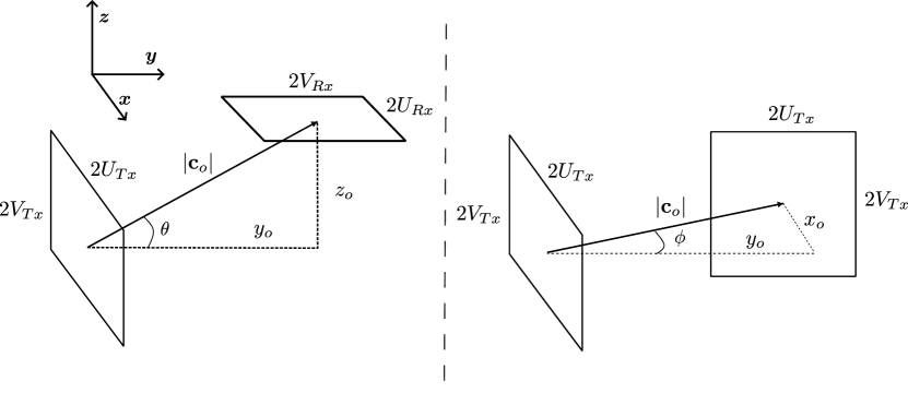
Figure 2: (left) Case study $x_{o}=0$, $\alpha=0$, $\beta=\pi/2$: The transmitting HoloS is deployed on a wall; the receiving HoloS is deployed on the ceiling. (right) Case study $z_{o}=0$, $\beta=0$, $\alpha=\pi/2$: The transmitting HoloS is deployed on a wall; the receiving HoloS is deployed on a perpendicular wall.

VI-B Case Studies

In this section, we show that the setting $\tau_{12}=\tau_{21}=0$ corresponds to network deployments that are useful in wireless communications, which are not limited to the paraxial deployment (i.e., the center-points of the HoloSs are aligned). As examples, we focus on two (non-paraxial) case studies.

By direct inspection of $\tau_{12}$ and $\tau_{21}$, we conclude that they are both equal to zero if (i) $x_{o}=0$ and $\alpha=0$ or (ii) $z_{o}=0$ and $\beta=0$. Therefore, we analyze these two network deployments. In both cases, we assume $\sigma_{1}=\sigma_{2}=1$ (quartic approximation).

VI-B1 Case study $x_{o}=0$ and $\alpha=0$

An illustrative example of this case study is given in Fig. 2 when $\beta=\pi/2$. Fig. 2 corresponds to a scenario where the transmitting HoloS is deployed on a wall and the receiving HoloS is deployed on the ceiling within a room, which is a typical non-paraxial setup.

Departing from the definitions of $\tau_{11}$ and $\tau_{22}$ in (21), we obtain $\tau_{11}=-1$ and ${\tau_{22}}=-{\cos^{2}}{\theta_{o}}\cos\beta+\sin{\theta_{o}}\cos{\theta_{o}}\sin\beta$, by taking into account that $x_{o}=0$ implies $\phi_{o}=0$. Therefore, the number of eDoF in (24) ultimately depends on $\left|{{\tau_{22}}}\right|$, i.e., ${N_{{\rm{eDoF}}}}\propto\left|{{\tau_{22}}}\right|$, and hence it explicitly depends on the angle of elevation $\theta_{o}$. Based on these considerations, the following remarks concerning the optimal deployment of the HoloSs, as a function of relevant design parameters, can be made.

Remark 2. According to Proposition 2, the number of DoF in (24) is maximized if the receiving HoloS is tilted towards the center-point of the transmitting HoloS by an angle equal to $\beta^{\mathrm{opt}}=-\theta_{o}$. Thus, it is insightful to compare the number of eDoF when the receiving HoloS is deployed parallel to the transmitting HoloS, i.e., $\beta=0$, the receiving HoloS is tilted towards the transmitting HoloS by the optimal angle, i.e., $\beta={\beta^{{\rm{opt}}}}$, and the receiving HoloS is deployed perpendicular to the transmitting HoloS, i.e., $\beta=\pi/2$, as shown in Fig. 2. We obtain ${N_{{\rm{eDoF}}}}\left({\beta=0}\right)\propto{\cos^{2}}{\theta_{o}}$, ${N_{{\rm{eDoF}}}}\left({\beta={\beta^{{\rm{opt}}}}}\right)\propto\cos{\theta_{o}}$, and ${N_{{\rm{eDoF}}}}\left({\beta=\pi/2}\right)\propto\sin{\theta_{o}}\cos{\theta_{o}}$, respectively. We conclude that, given $\theta_{o}$, optimizing the tilt of the receiving HoloS increases the number of eDoF. Also, we see that deploying the HoloSs parallel to each other (i.e., $\beta=0$) increases the number of eDoF, as compared with deploying them perpendicular to each other (i.e., $\beta=\pi/2$), when $0\leq{\theta_{o}}\leq\pi/4$. When $\pi/4\leq{\theta_{o}}\leq\pi/2$, on the other hand, the opposite holds true. In agreement with Prop. 2, however, the paraxial deployment provides the best performance, since $\left|{{\tau_{22}}}\right|=1$ in this case.

Remark 3. By computing the first-order derivative of $\tau_{22}$ as a function of $\theta$ and setting it equal to zero, we evince that the number of eDoF in (24) is maximized if the angle of elevation of the center-point of the receiving HoloS with respect to the center-point of the transmitting HoloS is equal to the negative half of the tilt of the receiving HoloS, i.e., $\theta_{o}^{{\rm{opt}}}=-\beta/2$. Thus, it is insightful to compare the number of eDoF when the receiving HoloS is deployed at different angles of elevation, including $\theta_{o}=0$, $\theta_{o}=\theta_{o}^{{\rm{opt}}}$, and $\theta_{o}=\pi/2$. We obtain ${N_{{\rm{eDoF}}}}\left({{\theta_{o}}=0}\right)\propto\cos\beta$, ${N_{{\rm{eDoF}}}}\left({{\theta_{o}}=\theta_{o}^{{\rm{opt}}}}\right)\propto 0.5\left({1+\cos\beta}\right)$, and ${N_{{\rm{eDoF}}}}\left({{\theta_{o}}=\pi/2}\right)\to 0$, respectively. It is worth noting that the case study ${{\theta_{o}}=\pi/2}$ results in a number of eDoF equal to one, because of the $\max\{\cdot\}$ operator in (24). We conclude that, given $\beta$, optimizing the angle of elevation of the receiving HoloS increases the number of eDoF. If $\beta=\pi/2$ (as shown in Fig. 2), e.g., the position of the receiving HoloS can be optimized at ${{\theta_{o}}=\theta_{o}^{{\rm{opt}}}}$, so as to have a number of eDoF greater than one, as we would have, on the other hand, if ${\theta_{o}}=0$.

VI-B2 Case study $z_{o}=0$ and $\beta=0$

An illustrative example of this case study is given in Fig. 2 when $\alpha=\pi/2$. Fig. 2 corresponds to a scenario where the transmitting HoloS is deployed on a wall and the receiving HoloS is deployed on a perpendicular wall, which is a typical non-paraxial setup.

Departing from the definitions of $\tau_{11}$ and $\tau_{22}$ in (21), we obtain ${\tau_{11}}=-{\cos^{2}}{\phi_{o}}\cos\alpha+\sin{\phi_{o}}\cos{\phi_{o}}\sin\alpha$ and $\tau_{22}=-1$, by taking into account that $z_{o}=0$ implies $\theta_{o}=0$. Thus, the number of eDoF in (24) ultimately depends on $\left|{{\tau_{11}}}\right|$, i.e., ${N_{{\rm{eDoF}}}}\propto\left|{{\tau_{11}}}\right|$, and it explicitly depends on azimuth angle $\phi_{o}$.

We note that the case study $z_{o}=0$ and $\beta=0$ is mathematically equivalent to the case study $x_{o}=0$ and $\alpha=0$, upon replacing ${\theta_{o}}\mapsto{\phi_{o}}$ and $\beta\mapsto\alpha$. Therefore, Remarks 2 and 3 apply to the corresponding angles: The angles of rotation and azimuth of the center-point of the receiving HoloS can be appropriately optimized to maximize the number of eDoF.

The considered case studies unveil that the proposed mathematical framework constitutes a general tool for optimizing the deployment of HoloSs, maximizing the number of eDoF, and gaining engineering insights on the impact of different network deployments on the performance limits of holographic MIMO.

VII Numerical Results

In this section, we show some numerical results to validate the main findings of the analysis. Unless stated otherwise, the considered setup is: $f_{c}=28$ GHz (i.e., $\lambda=1.07$ cm), $2U_{Tx}=2U_{Rx}=2V_{Tx}=2V_{Rx}=32\lambda=34.24$ cm, $|\mathbf{c}_{o}|=256\lambda=2.74$ m. Similar to Sec. VI-B, we consider $x_{o}=|\mathbf{c}_{o}|\sin\phi_{o}\cos\theta_{o}$, $y_{o}=|\mathbf{c}_{o}|\cos\phi_{o}\cos\theta_{o}$ $z_{o}=|\mathbf{c}_{o}|\sin\theta_{o}$, and we set $\phi_{o}=\pi/6$. Different values of $\theta_{o}$, $\alpha$, and $\beta$ are analyzed, as case studies. As for $\alpha$ and $\beta$, we consider the paraxial deployment as a reference, as well as the deployments in Fig. 2, since they are of interest in wireless communications.

VII-A Accuracy of the Quartic Approximation

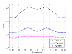
Figure 3: Approximation accuracy – $\alpha=0$, $\beta=0$.

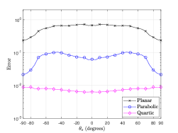
Figure 4: Approximation accuracy – $\alpha=0$, $\beta=\pi/2$.

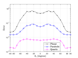
Figure 5: Approximation accuracy – $\alpha=\pi/2$, $\beta=0$.

In Figs. 5, 5, 5, we analyze the accuracy provided by the quartic approximation, and compare it against the accuracy provided by the parabolic and far-field (planar) approximations. The accuracy is expressed in terms of the total relative error committed in approximating the kernel in (11)

$$\text{error}=\int_{\mathcal{S}_{T}}\int_{\mathcal{S}_{T}}\left|\frac{{G}_{Tx}^{\mathrm{(e)}}(\mathbf{r}_{Tx},\mathbf{r}_{Tx}^{\prime})-{G}_{Tx}^{\mathrm{(a)}}(\mathbf{r}_{Tx},\mathbf{r}_{Tx}^{\prime})}{{G}_{Tx}^{\mathrm{(e)}}(\mathbf{r}_{Tx},\mathbf{r}_{Tx}^{\prime})}\right|d\mathbf{r}_{Tx}d\mathbf{r}_{Tx}^{\prime}$$

where ${G}_{Tx}^{\mathrm{(\cdot)}}(\mathbf{r}_{Tx},\mathbf{r}_{Tx}^{\prime})=F_{Tx}(\mathbf{r}_{Tx})F_{Tx}^{*}(\mathbf{r}_{Tx}^{\prime}){\bar{G}}_{Tx}^{(\cdot)}(\mathbf{r}_{Tx},\mathbf{r}_{Tx}^{\prime})$, with ${G}_{Tx}^{\mathrm{(e)}}(\cdot)$ and ${G}_{Tx}^{\mathrm{(a)}}(\cdot)$ denoting the exact and approximated kernels in (11) and (IV-B), respectively, and $F_{Tx}(\cdot)$ is in (14).

The numerical analysis confirms the better accuracy provided by the proposed quartic approximation, and the limitations of the parabolic approximation in non-paraxial setups.

VII-B Accuracy of the Number of eDoF in (24)

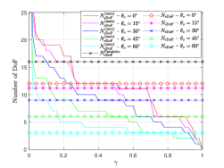
Figure 6: $N_{\rm eDoF}$ in (24) – $\alpha=0$, $\beta=0$.

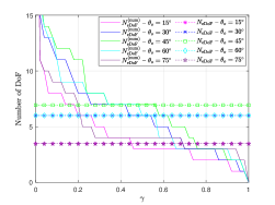
Figure 7: $N_{\rm eDoF}$ in (24) – $\alpha=0$, $\beta=\pi/2$.

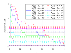
Figure 8: $N_{\rm eDoF}$ in (24) – $\alpha=\pi/2$, $\beta=0$.

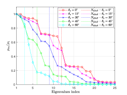
Figure 9: Eigenvalues – Solid lines with markers: Numerical solution.

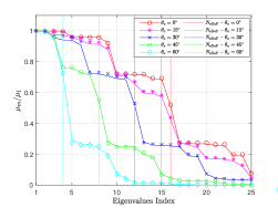
Figure 10: Eigenvalues – Solid lines: Numerical solution. Markers: PSWF in (15).

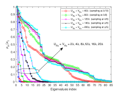
Figure 11: Eigenvalues – Solid lines: Sampling at $\lambda/16$. Markers: Sampling at $\lambda/2$ (if size $\leq 20\lambda$).

In Figs. 8, 8, 8, 11, we analyze the accuracy of (24), and compare it against numerical simulations and the paraxial approximation (by setting ${\sigma_{1}}=1$ and ${\sigma_{2}}=0$). Based on Remark 1, the number of eDoF is computed (by simulations) as $N_{{\rm{eDoF}}}^{(\rm{num})}=\max\left\{{m:{\gamma\mu_{1}}\leq{\mu_{m}}\leq{{\mu}_{1}}}\right\}$, where $\mu_{m}$ is the $m$th eigenvalue, $\mu_{1}$ is the largest (first) eigenvalue, and $\gamma$ is the level of approximation accuracy (according to Def. 8).

The quartic approximation provides accurate estimates for $N_{\rm eDoF}$. Even though no theoretical result similar to (36) exists for general deployments, comparing numerical analysis and (24) shows that $N_{\rm eDoF}$ is a good estimate if the approximation accuracy is $\gamma\approx 0.5$, as for the PSWFs. The parabolic approximation provides, on the other hand, inaccurate estimates: $N_{\rm eDoF}$ would be equal to zero, based on (25), for the deployments in Figs. 8 and 8. In Fig. 11, we show the intensity of the eigenvalues. The setup is $\alpha=0$, $\beta=0$, and $\theta_{o}$ is varied. $N_{\rm eDoF}$ provides a good estimate of the number of eigenvalues whose intensity is greater than half of the largest eigenvalue.

VII-C Accuracy of the Number of eDoF in (35)

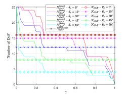
Figure 12: $N_{\rm eDoF}$ in (35) – $\alpha=0$, $\beta=0$.

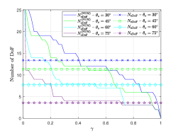
Figure 13: $N_{\rm eDoF}$ in (35) – $\alpha=0$, $\beta=\pi/4$.

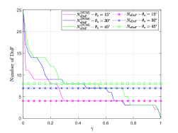
Figure 14: $N_{\rm eDoF}$ in (35) – $\alpha=0$, $\beta=\pi/2$.

In Figs. 14, 14, 14, 11, we analyze the accuracy of (28), and compare it against numerical simulations and the paraxial approximation, which are obtained as in Sec. VII-B.

The trends are similar to those observed in Figs. 8, 8, 8, 11. In this case, in addition, we see that the theoretical prediction in (36) is fulfilled. Also, Fig. 11 is obtained assuming the same setup as in Fig. 11. In this case, notably, the analytical estimate of the eigenvalues in (34) (markers) is compared against the numerical simulations, and a good accuracy is obtained.

VII-D Accuracy of the Number of eDoF in (28)

In Figs. 11 and 20, we analyze the accuracy of (28), similar to Sec. VII-B. As an example, we consider the first case study in Sec. V-B. The size of the transmitting HoloS is kept fixed to $2U_{Tx}=2V_{Tx}=4\lambda$, and the size of the receiving HoloS is varied. The transmission distance is $|\mathbf{c}_{o}|=32\lambda$, and $\theta_{o}=\pi/4$, $\phi_{o}=\pi/6$ as an example of non-paraxial setup. Due to the short distance and large size of the HoloSs, we consider a small spatial sampling for the numerical results. The spatial sampling is chosen in the range $\lambda/16$, for HoloSs of small-medium size ($U_{Rx}=V_{Rx}\leq 20\lambda$), and $\lambda/5$, for HoloSs of large size (e.g., $U_{Rx}=V_{Rx}=200\lambda$). This is due to the memory and computing requirements when solving the exact eigenproblem in (7).

From Fig. 11, we see that a spatial sampling at $\lambda/2$ is sufficient for small-medium HoloSs. Also, we note a sharp transition band, similar to previous case studies, but a large number of eigenvalues with a small intensity (especially if $0.5\leq\gamma\leq 0.1$). Fig. 20 confirms the inaccuracy of (24) for large-size HoloSs. Also, Fig. 20 confirms that (28) is an upper-bound for $N_{\rm{eDoF}}$ if the approximation accuracy is $\gamma=0.5$, and that there exists a large number of eigenvalues whose intensity is smaller than half of the largest eigenvalue. The estimate in (28) is well below the number of eigenvalues whose intensity is ten times smaller than the largest eigenvalue (i.e., $\gamma=0.1$). Thus, (28) is a suitable estimate for the number of eDoF. The development of tighter approximations for large-size HoloSs is an interesting open problem that deserves further investigation.

VII-E Accuracy of the Eigenfunctions in (32)

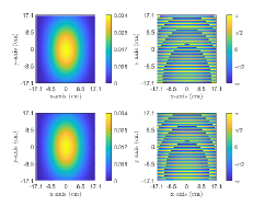
Figure 15: First eigenfunction – (top) Numerical. (bottom) Analytical. (left) Amplitude. (right) Phase.

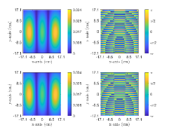
Figure 16: Third eigenfunction – (top) Numerical. (bottom) Analytical. (left) Amplitude. (right) Phase.

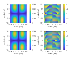
Figure 17: Fifth eigenfunction – (top) Numerical. (bottom) Analytical. (left) Amplitude. (right) Phase.

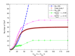
Figure 18: $N_{\rm eDoF}$ in (28) – $\alpha=0$, $\beta=0$, $\theta_{o}=\pi/4$.

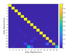
Figure 19: Orthonormality of the eigenfunctions.

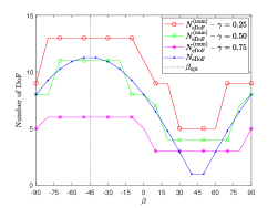
Figure 20: Optimal value of the tilt angle $\beta$.

In Figs. 17, 17, 17, 20, we analyze the accuracy of the optimal communication waveforms in (32), and compare them against those obtained by using numerical methods. As an example, we consider the setting $x_{o}=0$ and $\alpha=0$, which fulfills $\tau_{12}=\tau_{21}=0$. Specifically, we set $\beta=\pi/2$, $\theta=\pi/4$, and $\phi=0$. The PSWFs in (32) are computed by using [24], and the numerical waveforms are obtained by applying the singular value decomposition to the exact eigenproblem in (7).

The difference between the numerical and analytical eigenfunctions is almost not noticeable to the naked eye. This confirms the accuracy of (32) in typical non-paraxial deployments.

In Fig. 20, we analyze the orthonormality of the eigenfunctions in (32) when they are observed at the receiver. Each eigenfunction obtained from (32) is inserted into (1), and the electric field at the receiving HoloS is computed numerically. The resulting electric field is multiplied by each eigenfunction, and it is integrated across the HoloS (cross-correlation). We see that the orthonormal waveforms at the transmitting HoloS are still orthonormal at the receiving HoloS, even though they are obtained by applying the proposed quartic approximation. This further validates the proposed approach. Minor deviations are noticeable only for a few high-order modes.

VII-F Optimality of the Deployments in Remarks 2 and 3

In Fig. 20, we analyze the number of eDoF as a function of the tilt angle $\beta$. As an example, we consider the setting $x_{o}=0$ and $\alpha=0$ discussed in Remark 2. Similar results are obtained for Remark 3. The numerical estimates as a function of the estimation accuracy $\gamma$ are computed as in Sec. VII-B.

We see that the optimal solution identified in Remark 2 is consistent with the numerical simulations. In agreement with the figures illustrated already, we observe that the analytical framework closely matches the numerical simulations when the approximation accuracy is $\gamma\approx 0.5$. Also, we note that the optimal value of the tilt angle is independent of $\gamma$.

VIII Conclusion

We have introduced an analytical framework for computing the number of eDoF of holographic MIMO. The proposed approach relies on a quartic approximation for the wavefront of the electromagnetic waves, which makes it accurate in non-paraxial deployments. Also, the approach can be applied to surfaces of any size. For a class of network deployments that encompass several case studies of interest in wireless communications, we have identified the optimal communication waveforms. With the aid of extensive numerical simulations, we have validated the accuracy of the proposed approach.

Appendix A – Proof of Lemma 9

Given the parametrization of the HoloSs in (17) and (18), we obtain $\delta\rho_{1}\left({\bf{r}}_{Tx}\right)=u_{i}^{2}+v_{i}^{2}-2(x_{o}u_{i}+z_{o}v_{i})$, $\delta{\rho_{3}}\left({{{\bf{r}}_{Tx}},{\bf{r}}_{Tx}^{\prime},{{\bf{r}}_{Rx}}}\right)=-2[(u_{i}-u_{i}^{\prime})(u_{o}\cos{\alpha}-v_{o}\sin\beta\sin\alpha)+(v_{i}-v_{i}^{\prime})v_{o}\cos{\beta}]$, $\delta\rho_{1}^{2}\left({\bf{r}}_{Tx}\right)=4\left(x_{o}u_{i}+z_{o}v_{i}\right)^{2}$ and $\delta{\rho_{3}^{2}}\left({{{\bf{r}}_{Tx}},{\bf{r}}_{Tx}^{\prime},{{\bf{r}}_{Rx}}}\right)=-8x_{o}[(x_{o}\cos\alpha+y_{o}\sin\alpha)u_{o}+(-x_{o}\sin\beta\sin\alpha+y_{o}\sin\beta\cos\alpha+z_{o}\cos\beta)v_{o}](u_{i}-u_{i}^{\prime})-8z_{o}[(x_{o}\cos\alpha+y_{o}\sin\alpha)u_{o}+(-x_{o}\sin\beta\sin\alpha+y_{o}\sin\beta\cos\alpha+z_{o}\cos\beta)v_{o}](v_{i}-v_{i}^{\prime})$. By inserting these expressions in (14), (20) immediately follows. As far as (IV-B) is concerned, we obtain

$$\bar{G}_{Tx}\left(\bf{r}_{Tx},\bf{r}_{Tx}^{\prime}\right)\approx\int_{-U_{Rx}}^{U_{Rx}}\int_{-V_{Tx}}^{V_{Tx}}\\ \exp\bigg{\{}j\frac{k_{0}}{|\mathbf{c}_{o}|}\left[(\tau_{11}(u_{i}-u_{i}^{\prime})+\tau_{12}(v_{i}-v_{i}^{\prime}))u_{o}\right.\\ \left.+(\tau_{21}(u_{i}-u_{i}^{\prime})+\tau_{22}(v_{i}-v_{i}^{\prime}))v_{o}\right]\bigg{\}}dv_{o}du_{o}$$ (37)

where $\tau_{11}$, $\tau_{12}$, $\tau_{21}$, $\tau_{22}$ are given in Sec. V. Since $\int_{-a}^{a}\exp(jbx)dx=2a\operatorname{sinc}(ba/\pi)$, the expression in (21) follows by noting that $k_{0}=2\pi/\lambda$ and $A_{Rx}=(2U_{Rx})(2V_{Rx})$.

Appendix B – Proof of Lemma 10

To compute the Fourier transform of ${h_{G}}\left({{{\bf{r}}_{Tx}}}\right)={{\bar{G}}_{Tx}}\left({{{\bf{r}}_{Tx}};{\bf{r}}_{Tx}^{\prime}=0}\right)$ in (21), we first compute the Fourier transform of $h_{0}(\mathbf{q})=A_{Rx}\operatorname{sinc}(s)\operatorname{sinc}(t)$, and then apply the linear transformation $h_{G}(\mathbf{r}_{Tx})=h_{0}(\mathbf{q}=\mathbf{A}\mathbf{r}_{Tx})$, where

$$\mathbf{A}=\begin{bmatrix}U_{o}\tau_{11}&U_{o}\tau_{12}\\ V_{o}\tau_{21}&V_{o}\tau_{22}\end{bmatrix}\,.$$ (38)

Specifically, the Fourier transform of $h_{0}(\mathbf{q})$ is [25, Tab. 2.2]

$$H_{0}(\mathbf{k}_{q})=\pi^{2}A_{Rx}\operatorname{rect}\left(\frac{k_{s}}{2\pi}\right)\operatorname{rect}\left(\frac{k_{t}}{2\pi}\right)\,.$$ (39)

Applying [25, Property 2.6], the Fourier transform of $h_{G}(\mathbf{r}_{Tx})=h_{0}(\mathbf{q}=\mathbf{A}\mathbf{r}_{Tx})$ is $H_{G}(\mathbf{k}_{Tx})=H_{0}(\mathbf{k}_{q}=\mathbf{A}^{-T}\mathbf{k}_{Tx})$ $/|\det{\mathbf{A}}|$, where ${{\bf{A}}^{-T}}={\left({{{\bf{A}}^{-1}}}\right)^{T}}$. $H_{G}(\mathbf{k}_{Tx})$ is given in (V).

We see that $H_{0}(\mathbf{k}_{q})$ is an ideal low-pass filter that is non-zero in the set ${{\mathcal{H}}_{0}}=\left\{{\left({{k_{s}},{k_{t}}}\right):\left|{{k_{s}}}\right|\leq\pi,\left|{{k_{t}}}\right|\leq\pi}\right\}$, whose Lebesgue measure is ${m_{0}}=m\left({{{\mathcal{H}}_{0}}}\right)=4{\pi^{2}}$. We refer to ${{\mathcal{H}}_{0}}$ as the spatial bandwidth of $H_{0}(\mathbf{k}_{q})$. The spatial bandwidth of $H_{G}(\mathbf{k}_{Tx})$ can be directly obtained from the transformation $\mathbf{k}_{q}=\mathbf{A}^{-T}\mathbf{k}_{Tx}$ applied to (39) in the wavenumber domain. By applying, therefore, the change of variables $\mathbf{k}_{Tx}=\mathbf{A}^{T}\mathbf{k}_{q}$, the spatial bandwidth of $H_{G}(\mathbf{k}_{Tx})$ can be formulated as

$$m_{G} =m(\mathcal{H}_{G})=\int_{-\pi}^{\pi}\int_{-\pi}^{\pi}|\det{\mathbf{A}^{T}}|dk_{s}dk_{t}$$ (40)

$$=4\pi^{2}|\det{\mathbf{A}^{T}}|=4\pi^{2}\frac{A_{Rx}}{\lambda^{2}|\mathbf{c}_{o}|^{2}}|\tau_{11}\tau_{22}-\tau_{12}\tau_{21}|$$ (41)

since $A_{Rx}=(2U_{Rx})(2V_{Rx})$.

Appendix C – Proof of Proposition 2

The function $|\Upsilon(\alpha,\beta,x_{o},y_{o},z_{o})|$ is not differentiable, but it has the same critical points as $\Upsilon(\alpha,\beta,x_{o},y_{o},z_{o})$. Setting $\sigma_{1}=\sigma_{2}=1$, we obtain $\Upsilon(\alpha,\beta,x_{o},y_{o},z_{o})=(y_{o}^{2}\cos\alpha\cos\beta-y_{o}z_{o}\sin\beta-x_{o}y_{o}\sin\alpha\cos\beta)|\mathbf{c}_{o}|^{-2}$. Therefore, we need to analyze the partial derivatives of $f(\alpha,\beta)=y_{o}^{2}\cos\alpha\cos\beta-y_{o}z_{o}\sin\beta-x_{o}y_{o}\sin\alpha\cos\beta$. By computing ${{\partial f\left({\alpha,\beta}\right)}\mathord{\left/{\vphantom{{\partial f\left({\alpha,\beta}\right)}{\partial\alpha}}}\right.\kern-1.2pt}{\partial\alpha}}$ and ${{\partial f\left({\alpha,\beta}\right)}\mathord{\left/{\vphantom{{\partial f\left({\alpha,\beta}\right)}{\partial\beta}}}\right.\kern-1.2pt}{\partial\beta}}$, and setting them to zero, we obtain

$$\tan\alpha^{\mathrm{opt}}=-\frac{x_{o}}{y_{o}}$$ (42)

$$\tan\beta^{\mathrm{opt}}=\frac{z_{o}}{x_{o}\sin\alpha^{\mathrm{opt}}-y_{o}\cos\alpha^{\mathrm{opt}}}\,.$$ (43)

Using the trigonometric identities $\sin x=\frac{\tan x}{\sqrt{1+\tan^{2}x}}$ and $\cos x=\frac{1}{\sqrt{1+\tan^{2}x}}$ in (42) and (43), we can express the angles $\alpha^{\mathrm{opt}}$ and $\beta^{\mathrm{opt}}$ as in (26). Furthermore, we can obtain the maximum number of DoF by inserting (26) into (24).

Appendix D – Proof of Proposition 3

Assume the HoloSs are partitioned into smaller sub-surfaces, such that, for each pair of transmitting and receiving sub-surfaces, the distance between the center-points is larger than their sizes. Denote the generic transmitting and receiving sub-HoloSs as $d{{\mathcal{S}}_{i}}$ and $d{{\mathcal{S}}_{o}}$, and their areas as $dA_{i}=m(d{{\mathcal{S}}_{i}})$ and $dA_{o}=m(d{{\mathcal{S}}_{o}})$, respectively. Also, denote their center-points as $\mathbf{r}^{c}_{i}=\left({x^{c}_{i},y^{c}_{i},z^{c}_{i}}\right)$ and $\mathbf{r}^{c}_{o}=\left({x^{c}_{o},y^{c}_{o},z^{c}_{o}}\right)$. Then, the integrals in (7) and (9) can be expressed in terms of the ensemble of sub-HoloSs, as $\int_{\mathcal{S}}{}\to\int_{\bigcup{d{\mathcal{S}}}}{}\to\sum{\int_{d{\mathcal{S}}}{}}$, ensuring $\left|\mathbf{r}^{c}_{o}-\mathbf{r}^{c}_{i}\right|\gg\sqrt{dA}$ for each integral of the summation. This is, in general, possible, for every distance $\left|\mathbf{r}^{c}_{o}-\mathbf{r}^{c}_{i}\right|$, by considering sufficiently (in the limit infinitesimally) small sub-HoloSs.

In general terms, the rationale of the proof can be stated as follows. Based on the considered partitions and on the results in App. A, the kernel ${{\bar{G}}_{Tx}}\left({{{\bf{r}}_{Tx}},{\bf{r}}_{Tx}^{\prime}}\right)$ can be expressed as the summation of terms equal to (21) for each pair of sub-HoloSs $\left({{\rm{d}}{{\mathcal{S}}_{i}},{\rm{d}}{{\mathcal{S}}_{o}}}\right)$, and (24) can hence be applied to any pair of such sub-HoloSs. In other words, the kernel in (15) can be formulated as the summation of disjoint transmitting and receiving sub-HoloSs. The Fourier transform, in the wavenumber domain, of each term of the summation is, however, not disjoint in general, even though each term of the kernel acts as an ideal filter, according to (39) in App. B. From Lemma 8, hence, the number of eDoF can be obtained from the Lesbegue measure of the ensemble of transmitting sub-HoloSs, expressed in terms of $\left\{{{\rm{d}}{{\mathcal{S}}_{i}}}\right\}$, and the Lesbegue measure of the Fourier transform, in the wavenumber domain, of the compact self-adjoint operator in (15) expressed in terms of the ensemble of transmitting and receiving sub-HoloSs $\left\{{{\rm{d}}{{\mathcal{S}}_{i}}},{{\rm{d}}{{\mathcal{S}}_{o}}}\right\}$.

In mathematical terms, considering all the sub-HoloSs $\left\{{{\rm{d}}{{\mathcal{S}}_{i}}},{{\rm{d}}{{\mathcal{S}}_{o}}}\right\}$, and utilizing the same notation as in Sec. III-B and App. B, Lemma 8 leads to the upper-bound

$$N_{\mathrm{eDoF}}\leq{(2\pi)^{-2}}\sum\nolimits_{o}\sum\nolimits_{i}m\left({{\mathcal{H}}_{{G_{o,i}}}}\right)m\left({d{{\mathcal{S}}_{i}}}\right)$$ (44)

where $\mathcal{H}_{G_{o,i}}$ denotes the Fourier transform of the self-adjoint operator corresponding to the pair $\left({{\rm{d}}{{\mathcal{S}}_{i}}},{{\rm{d}}{{\mathcal{S}}_{o}}}\right)$ of transmitting and receiving sub-HoloSs, and the inequality accounts for the fact that the supports of the Fourier transforms of $\left\{{{{\mathcal{H}}_{{G_{o,i}}}}}\right\}$, as defined in App. B for each pair of sub-HoloSs, are overlapping in the wavenumber domain, even though the transmitting and receiving sub-HoloSs are spatially disjoint. Also, based on App. B, we have $m\left({{{\mathcal{H}}_{{G_{o,i}}}}}\right)=4\pi^{2}\frac{dA_{o}|\Theta(\mathbf{r}^{c}_{o}-\mathbf{r}^{c}_{i})|}{\lambda^{2}|\mathbf{r}^{c}_{o}-\mathbf{r}^{c}_{i}|^{2}}$ with $\Theta(\mathbf{r}^{c}_{o}-\mathbf{r}^{c}_{i})$ given in (29). The proof follows by replacing the sums in (44) with integrals, and integrating over the HoloSs.

Appendix E – Proof of Proposition 4

Consider ${{\bar{G}}_{Tx}}\left({{{\bf{r}}_{Tx}},{\bf{r}}_{Tx}^{\prime}}\right)$ in (21) by setting $\tau_{12}=\tau_{21}=0$. The eigenproblem in (15) simplifies to

$${{{\mu_{m}}}}{{\bar{\phi}}_{m}}\left({{u_{i}},{v_{i}}}\right) ={\left|{{{\bar{g}}_{i,o}}\left({{{\bf{c}}_{Tx}};{{\bf{c}}_{Rx}}}\right)}\right|^{2}}$$ (45)

$$\times\int_{-{U_{Tx}}}^{{U_{Tx}}}{\int_{-{V_{Tx}}}^{{V_{Tx}}}{{A_{Rx}}f\left({u_{i}^{\prime},v_{i}^{\prime}}\right){{\bar{\phi}}_{m}}\left({{u_{i}^{\prime}},{v_{i}^{\prime}}}\right)du_{i}^{\prime}dv_{i}^{\prime}}}$$

where $f\left({u_{i}^{\prime},v_{i}^{\prime}}\right)={\rm{sinc}}\left({{U_{o}}{\tau_{11}}\left({{u_{i}}-u_{i}^{\prime}}\right)}\right){\rm{sinc}}\left({{V_{o}}{\tau_{22}}\left({{v_{i}}-v_{i}^{\prime}}\right)}\right)$.

Let us define ${{{{\bar{\mu}}_{m,i,o}}}}=A_{Rx}^{-1}{\left|{{{\bar{g}}_{i,o}}\left({{{\bf{c}}_{Tx}};{{\bf{c}}_{Rx}}}\right)}\right|^{-2}}{{{\mu_{m}}}}$, ${{{{\bar{\mu}}_{m,i,o}}}}={{{{\bar{\mu}}_{m,i,o,u}}}}{{{{\bar{\mu}}_{m,i,o,v}}}}$, and let us assume, without loss of generality, to look for eigenfunctions that can be written as ${{\bar{\phi}}_{m}}\left({{u_{i}},{v_{i}}}\right)={{\bar{\phi}}_{m,u}}\left({{u_{i}}}\right){{\bar{\phi}}_{m,v}}\left({{v_{i}}}\right)$. Then, the eigenproblem in (45) boils down to solving the two eigenproblems

$${{\tilde{\mu}}_{m,i,o,u}}{{\bar{\phi}}_{m,u}}\left({{u_{i}}}\right)=\int_{-{U_{Tx}}}^{{U_{Tx}}}{\frac{{\sin\left({\pi{U_{o}}{\tau_{11}}\left({{u_{i}}-u_{i}^{\prime}}\right)}\right)}}{{\pi\left({{u_{i}}-u_{i}^{\prime}}\right)}}{{\bar{\phi}}_{m,u}}\left({{u_{i}^{\prime}}}\right)du_{i}^{\prime}}$$

$${{\tilde{\mu}}_{m,i,o,v}}{{\bar{\phi}}_{m,v}}\left({{v_{i}}}\right)=\int_{-{V_{Tx}}}^{{V_{Tx}}}{\frac{{\sin\left({\pi{V_{o}}{\tau_{22}}\left({{v_{i}}-v_{i}^{\prime}}\right)}\right)}}{{\pi\left({{v_{i}}-v_{i}^{\prime}}\right)}}{{\bar{\phi}}_{m,v}}\left({{v_{i}^{\prime}}}\right)dv_{i}^{\prime}}$$

where ${{\tilde{\mu}}_{m,i,o,u}}={U_{o}}{\tau_{11}}{{\bar{\mu}}_{m,i,o,u}}$ and ${{\tilde{\mu}}_{m,i,o,v}}={V_{o}}{\tau_{22}}{{\bar{\mu}}_{m,i,o,v}}$. The proof follows from [23, Eq. (11)].

References

• [1] C. Huang et al., “Holographic MIMO surfaces for 6G wireless networks: Opportunities, challenges, and trends,” IEEE Wirel. Commun., vol. 27, no. 5, pp. 118–125, 2020.
• [2] J. An et al., “A tutorial on holographic MIMO communications - Part I, II, III,” IEEE Commun. Lett., pp. 1–1, 2023.
• [3] M. Di Renzo et al., “LoS MIMO-arrays vs. LoS MIMO-surfaces,” in Proc. 2023 European Conf. Antennas and Propag., 2023, pp. 1–5.
• [4] D. Dardari and N. Decarli, “Holographic communication using intelligent surfaces,” IEEE Commun. Mag., vol. 59, no. 6, pp. 35–41, 2021.
• [5] E. Telatar, “Capacity of multi-antenna gaussian channels,” European Trans. Telecommun., vol. 10, no. 6, pp. 585–595, 1999.
• [6] D. Miller, “Waves, modes, communications, and optics: A tutorial,” Adv. Opt. Photon., vol. 11, no. 3, pp. 679–825, Sep. 2019.
• [7] A. Pinkus, n-Widths in Approximation Theory.   Springer Berlin, 1985.
• [8] M. Franceschetti, Wave Theory of Information.   Cambridge Univ., 2017.
• [9] ——, “On Landau’s eigenvalue theorem and information cut-sets,” IEEE Trans. Inform. Theory, vol. 61, no. 9, pp. 5042–5051, Sep. 2015.
• [10] A. Pizzo et al., “On Landau’s eigenvalue theorem for line-of-sight MIMO channels,” IEEE Wirel. Comm. Let., no. 12, pp. 2565–2569, 2022.
• [11] M. D. Migliore, “On the role of the number of degrees of freedom of the field in MIMO channels,” IEEE Trans. Antennas Propag., vol. 54, no. 2, pp. 620–628, 2006.
• [12] D. Miller, “Communicating with waves between volumes: evaluating orthogonal spatial channels and limits on coupling strengths,” Appl. Opt., vol. 39, no. 11, pp. 1681–1699, Apr. 2000.
• [13] R. Piestun and D. Miller, “Electromagnetic degrees of freedom of an optical system,” J. Opt. Soc. Am. A, vol. 17, pp. 892–902, May 2000.
• [14] D. Dardari, “Communicating with large intelligent surfaces: Fundamental limits and models,” IEEE J. Sel. Areas Commun., vol. 38, Nov. 2020.
• [15] N. Decarli et al., “Communication modes with large intelligent surfaces in the near field,” IEEE Access, vol. 9, pp. 165 648–165 666, 2021.
• [16] D. Porter and D. Stirling, Integral equations.   Cambridge Univ., 1990.
• [17] H. J. Landau, “On Szegö’s eingenvalue distribution theorem and non-hermitian kernels,” J. d'Analyse Math., no. 1, pp. 335–357, 1975.
• [18] H. Do et al., “Parabolic wavefront model for line-of-sight MIMO channels,” IEEE Trans. Wireless Commun., pp. 1–1, 2023.
• [19] S. Yuan et al., “Electromagnetic effective degree of freedom of a MIMO system in free space,” IEEE Antennas Wirel. Propag. Lett., vol. 21, no. 3, pp. 446–450, 2022.
• [20] H. Do et al., “Terahertz line-of-sight MIMO communication: Theory and practical challenges,” IEEE Commun. Mag., vol. 59, pp. 104–9, 2021.
• [21] G. Bartoli et al., “Spatial multiplexing in near field MIMO channels with reconfigurable intelligent surfaces,” IET Sig. Proces., vol. 17, 2023.
• [22] W. C. Chew, Waves and Fields in Inhomogenous Media.   Wiley, 1999.
• [23] D. Slepian and H. O. Pollak, “Prolate spheroidal wave functions, Fourier analysis and uncertainty – I,” Bell System Technical Journal, vol. 40, no. 1, pp. 43–63, Jan. 1961.
• [24] R. R. Lederman, “Numerical algorithms for the computation of generalized prolate spheroidal functions,” 2017. [Online]. Available: https://arxiv.org/abs/1710.02874.
• [25] E. Dubois, Multidimensional Signal and Color Image Processing Using Lattices.   John Wiley & Sons, 2019.