Bound circumplanetary orbits under the influence of radiation pressure: Application to dust in directly imaged exoplanet systems

Abstract

We examine the population of simply periodic orbits in the Hill problem with radiation pressure included, in order to understand the distribution of gravitationally bound dust in orbit around a planet. We study a wide range of radiation pressure strengths, which requires the inclusion of additional terms beyond those discussed in previous analyses of this problem. In particular, our solutions reveal two distinct populations of stable wide, retrograde, orbits, as opposed to the single family that exists in the purely gravitational problem.

We use the result of these calculations to study the observational shape of dust populations bound to extrasolar planets, that might be observable in scattered or reradiated light. In particular, we find that such dusty clouds should be elongated along the star–planet axis, and that the elongation of the bound population increases with $\beta$, a measure of the strength of the radiation pressure.

As an application of this model, we consider the properties of the Fomalhaut system. The unusual orbital properties of the object Fomalhaut b can be explained if the observed light was scattered by dust that was released from an object in a quasi-satellite orbit about a planet located in, or near, the observed debris ring. Within the context of the model of Hayakawa & Hansen (2023), we find that the dust cloud around such a planet is still approximately an order of magnitude fainter than the limits set by current JWST data.

1 Introduction

The late stages of planetary system assembly are expected to result in the production of copious amounts of dust, which can be observed due to its capacity for reprocessing the light from the central star. Imaging of this population of dust, either in scattered light or thermal emission, can provide information on the properties of the planetary system by virtue of the sensitivity of the dust to the gravitational influence of the planets in the system.

In Hayakawa & Hansen (2023), we present a model for the origin of thin dust rings, in which the dust is generated in irregular satellite systems. As an alternative to the common ‘birth ring’ model for dust populations – which posits an origin in a ring of colliding planetesimals – we invoke a population of irregular satellites that generates the dust in the local vicinity of the host planet. The effect of radiation pressure from the central star is to shift the pseudopotential so that the collisional cascade is halted when dust escapes via the $L_{2}$ point and goes into orbit exterior to the planet. We demonstrated that this dust, regulated by the contours of the pseudopotential, naturally yields a thin dust ring similar to those observed in some systems.

Not all of the dust immediately escapes to orbits exterior to the planet. The question we wish to address in this paper is whether other aspects of the model are amenable to observation. In particular, we wish to calculate the expected properties of dust trapped in stable orbits, and whether they can be observed. Perhaps the best known example of a thin ring system is that in orbit around the star Fomalhaut (Kalas et al., 2005). There have also been claims of a planetary object in this system (Kalas et al., 2008; Kalas et al., 2013) although this has also been argued to be a dust cloud not associated with a planet (Currie et al., 2012; Galicher et al., 2013). The optical colors of this object suggest that the origin of the emission is scattered light from the primary, and Kennedy & Wyatt (2011) have suggested that the emission is the result of the collisional grinding down of a population of irregular satellites as posited above.

With the continued imaging of dust systems with HST, and the new capabilities of JWST becoming available, it is timely to reconsider the observability of dust bound, or in close orbit, around a planet, and to evaluate the expected signatures of this dust. Kennedy & Wyatt (2011) assume a distribution of dust that follows the orbits of the parent bodies about the planet, but particles in orbit around a planet will be subject to a variety of forces due to the radiation from the central star (Burns et al., 1979). Thus, in § 2 we define the version of the Photogravitational Hill problem needed for our case. In § 3 we then generalise the families of periodic orbits discussed in the original Hill problem by Henon (1969, 1970). In § 4 we then discuss how these orbits will manifest themselves in the full restricted three-body co-ordinate system. In § 5 we will discuss how this might be observable.

2 The Photogravitational Hill problem and Henon orbit families

The motion of dust in stellar or planetary systems is well suited to description in the limit of the restricted three-body problem, as the mass of dust particles is so small as to be accurately described as a test particle. In the case where the two massive bodies have a circular orbit, the dynamics is well-known and regulated by a conserved integral, the Jacobi integral (e.g. Murray & Dermott, 2000).

In the limit where the mass ratio $\mu$ between the two massive bodies is small, the dynamics in and around the sphere of influence of the less massive body can be fruitfully described in the context of the Hill problem (Hill, 1878a, b, c), wherein the dynamics is described in a co-ordinate frame centered on the smaller body (the planet). Henon (1969) presented an elegant analysis of the simply periodic orbits in a rescaled version of Hill’s problem in the limit where $\mu\rightarrow 0$. We wish here to revisit this question when the test particles are subject to a radiation pressure force from the central star, in order to describe the kinds of structures we might observe in a population of dust particles generated in close proximity to a planet.

In the original restricted three body problem, the massive bodies are separated by a semi-major axis of unity, and the center of mass in the co-rotating frame lies at $(0,0,0)$. If we move the origin of the co-ordinate system to the position of the planet (at $x=1-\mu$ and $y=0$), while simultaneously rescaling by $\mu$, we make the transformation $x=1-\mu+\mu^{1/3}\xi$, $y=\mu^{1/3}\eta$ and $z=\mu^{1/3}\zeta$, then the dynamics of the test particle is given by the equations

$$\ddot{\xi}-2\dot{\eta} = \frac{\beta}{\mu^{1/3}}+\left(3-2\beta-\frac{1}{\Delta^{3}}\right)\xi$$ (1)

$$\ddot{\eta}+2\dot{\xi} = \left(\beta-\frac{1}{\Delta^{3}}\right)\eta$$ (2)

$$\ddot{\zeta} = \left(\beta-1-\frac{1}{\Delta^{3}}\right)\zeta$$ (3)

where $\Delta^{2}=\xi^{2}+\eta^{2}+\zeta^{2}$ and we have dropped terms of higher order than $\mu^{1/3}$.

The dynamics of small particles in the restricted three body problem with radiation pressure has been described in many prior studies (Radzievskii, 1950, 1953; Schuerman, 1980; Simmons et al., 1985; Kushvah, 2008; Zotos, 2015, e.g). These analyses describe how the nature and stability of the Lagrangian equilibria evolve as the balance between gravity and radiation changes. Of particular interest to us are studies such as those by Markellos et al. (2000); Kanavos et al. (2002); Perdiou et al. (2012), which seek to describe the dynamics of particles near a planet while subject to radiation pressure, and which catalog the kinds of simply periodic orbits that arise.

However, these prior analyses of the ‘photogravitational problem’ make an approximation that is not appropriate for the application we seek. After the derivation of the above equations, the authors next step is to set $\beta=\mu^{1/3}Q_{1}$ and then take the limit $\mu\rightarrow 0$. This achieves an elegant rescaling that removes the mass dependance, in the same manner as the original classic work of Henon. However, it comes at a cost – in order for $Q_{1}$ to be a constant, $\beta\rightarrow 0$ in lockstep with $\mu$, so this only applies in the limit of small radiation pressure. This may be appropriate to applications such as describing the slow drift of spacecraft under the influence of stellar radiation (e.g. Giancotti et al., 2014; García Yárnoz et al., 2015), but it is not appropriate for describing the dynamics of dust, where the value of $\beta$ need not be infinitesimal.

Thus, we opt to keep $\beta$ finite, so that we may retain our ability to describe the dynamics of dust experiencing significant perturbations due to radiation pressure. This comes at the price that our description is no longer scale free – for a given $\beta$ we must also specify the value of $\mu$. We will, however, denote $Q^{\prime}=\beta/\mu^{1/3}$, as prior authors have done, to enable direct comparison between their results and ours.

The equations (1) and (2) still admit an equivalent of the Jacobi integral, now given as

$$C_{H}=\left(3-2\beta\right)\xi^{2}+\beta\eta^{2}+\left(\beta-1\right)\zeta^{2}+\frac{2}{\Delta}+2Q^{\prime}\xi-\dot{\xi}^{2}-\dot{\eta}^{2}-\dot{\zeta}^{2}$$ (4)

The difference between these equations and those of the traditional "photogravitational Hill problem" (Markellos et al., 2000; Kanavos et al., 2002) leads to some qualitative differences, as we will see below (although they represent a subset of the equilibria discussed in the more general restricted three body problem – Simmons et al. (1985)).

2.1 The Planar Equilibrium Points

The equilibrium points of the equations for the restricted three body problem define the transitions between different classes of dynamics. In the classic reduced three body problem, there are five equilibrium points – the Lagrange equilibria. Three of them – the colinear points $L_{1}$, $L_{2}$ and $L_{3}$ – lie on the line between the two gravitating masses in the co-rotating frame. The other two – the triangular points $L_{4}$ and $L_{5}$ – lie on either side of the secondary, at angles $\pm 60^{\circ}$.

The introduction of the radiation force shifts the positions of the equilibria and even introduces a new set of out-of-plane equilibria in the case of very strong radiation pressure (Radzievskii, 1950, 1953; Schuerman, 1980; Simmons et al., 1985). In order to understand the dynamics of dust particles, we wish to understand the implications of these changes in the Hill limit (i.e. when $\mu\ll 1$).

2.1.1 The Colinear Points

In the purely gravitational case ($\beta=0$), the equations in the Hill limit require $\eta=0$ for equilibria to exist. When we feed this condition into equation (1), we find that the colinear equilibria must satisfy

$$\xi^{3}+\frac{Q^{\prime}}{3-2\beta}\xi^{2}\mp\frac{1}{3-2\beta}=0$$ (5)

where the variation in the sign of the $Q^{\prime}$ term is due to the fact that $\Delta=\left|\xi\right|$ in this limit, which can be satisfied with two choice of sign for $\xi$.

In the case of $\beta=Q^{\prime}=0$, this yields the usual criterion $\xi=\pm 3^{1/3}$. Thus, the $L_{1}$ (negative $\xi$) and $L_{2}$ (positive $\xi$) equilibria lie at the same distance from the planet, on either side. The distant $L_{3}$ equilibrium vanishes in the limit.

For finite $\beta$, there are two different cubic equations, depending on the sign of the $Q^{\prime}$ term in equation (5), which will yield different values of $\left|\xi\right|$ on either side of the planet. Although cubic equations can yield multiple solutions, we note that not all of the solutions to equation (5) are valid, because only those roots that have the same sign as the coefficient of the $Q^{\prime}$ term are physically justified. The result of this is that the $L_{1}$ and $L_{2}$ points now lie at different distances from the planet. As we increase $\beta$, the $L_{1}$ point moves closer to the star and the $L_{2}$ point moves closer to the planet (see the comparison in Figure 2). The $L_{3}$ point also remains absent in this case. The character of the equipotentials also changes with finite $\beta$. Interior to $L_{2}$, the equipotentials remain centered on the planet, and so the zero-velocity contours restrict particles to circumplanetary motion. However, between the contour passing through $L_{2}$ and that passing through $L_{1}$, the zero-velocity curves open up and allow particles to escape to circumstellar orbits (this is the essential element that allows narrow dust rings to form in the model of Hayakawa & Hansen (2023)). As a result, the range of circumplanetary orbits is not bounded by $L_{1}$ and $L_{2}$ but by $L_{2}$ and a location $L_{2}^{\prime}$, representing the innermost edge of the pseudopotential contour that passes through $L_{2}$.

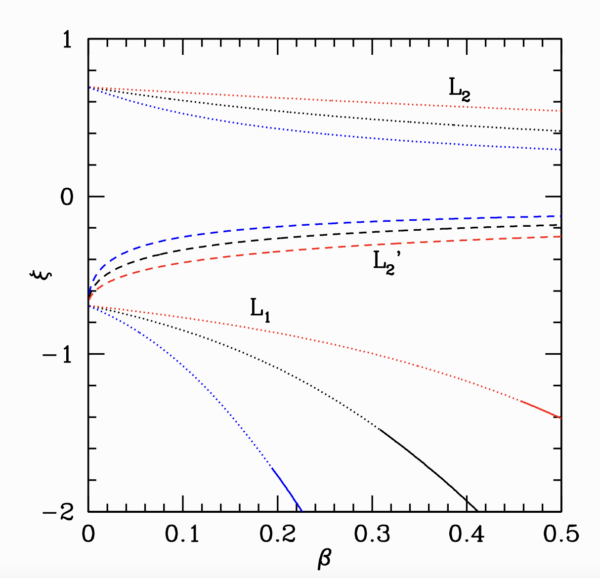
Figure 1: The dotted lines indicate the position of the saddle points $L_{1}$ and $L_{2}$, for the stated value of $\beta$. The $L_{1}$ curve turns solid at the point that it transitions from a saddle point to a potential minimum. The dashed contour indicates the location $L_{2}^{\prime}$ that marks the inner edge of the pseudopotential that passes through the $L_{2}$ point. The blue contours are for a mass ratio of $\mu=10^{-4}$, the black contours are for $\mu=10^{-3}$ and the red contours are for $\mu=10^{-2}$.

The nature of the equilibria will depend on the second derivatives of the pseudopotential. At low values of $\beta$, both the $L_{1}$ and $L_{2}$ points remain saddle points, as in the purely gravitational case. However, as $\beta$ increases, the $L_{1}$ point becomes a potential minimum when $\xi_{1}=-\beta^{-1/3}$ (this is when $\partial^{2}C_{H}/\partial\eta^{2}$ changes sign.) Figure 1 shows how the locations of $L_{1}$, $L_{2}$ and $L_{2}^{\prime}$ vary with the value of $\beta$ (for the case $\mu=0.001$).

2.1.2 Triangular Points in the Hill Problem

The presence of the $\beta$ dependant term in equation (2) enables the existence of additional equilibria beyond the colinear points. The new solution condition is $\Delta=\beta^{-1/3}$, which amounts to a condition on a specified distance from the planet. If we put this into equation (1) we must satisfy

$$\xi=-\frac{Q^{\prime}}{3(1-\beta)}$$ (6)

This yields something very like the $L_{4}$ and $L_{5}$ points, which don’t appear in the usual Hill or photogravitational Hill problems. This is a consequence of the $\beta$ dependant terms that remain even after the Taylor expansion of the potential about the location of the secondary. These terms break the usual symmetry that exists in the other versions of the Hill problem. As such, these points are not really a qualitatively new equilibrium, but they will have an influence on the kinds of periodic orbits we seek to describe below.

Figure 2 shows an example for $\beta=0.1$ and $Q=1$ (so $\mu=10^{-3}$) compared to the $\beta=0$ case for the same mass (in red). Thus, the $L_{1}$ point moves closer to the primary (farther from the planet) while the $L_{2}$ point moves closer to the planet. The new $L_{4}$ and $L_{5}$ points appear on the circle defined by the equation (6).

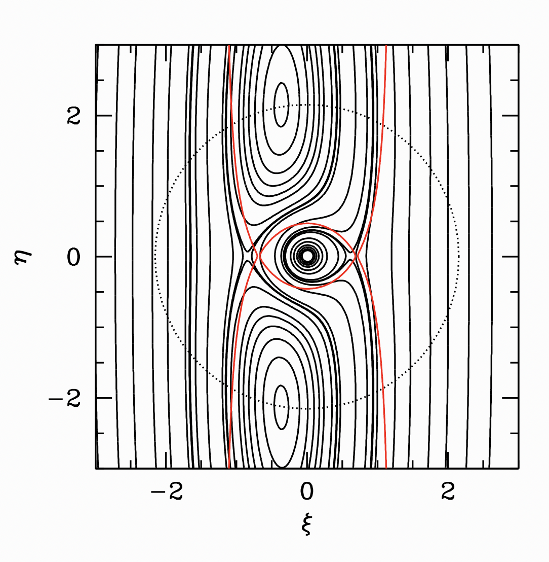
Figure 2: The black contours show equipotentials for the case of $\mu=10^{-3}$ and $\beta=0.1$ (so $Q^{\prime}=1$). The red contour shows the separatrix for the case of $\beta=0$ (and the same mass). The dotted line represents the circle upon which the Triangular equilibria are expected, and we can see the appearance of these points in the contours.

We dub these points the Triangular points because of their obvious connection to the $L_{4}$ and $L_{5}$ equilibria in the traditional restricted three body problem, but we must also note the features that do not exhibit an exact correspondence. In particular the angle these equilibria make with the primary–secondary axis is not $60^{\circ}$, and depends on $\beta$. As $\beta$ increases, these points move closer to the axis, and will converge when $\beta^{-1/3}=Q^{\prime}/3(1-\beta)$. Since $Q^{\prime}=\beta/\mu^{1/3}$, we can expand in the small parameter $\mu$ to derive an approximate criterion

$$\beta_{con}\sim 2.279\mu^{1/4}\left(1-1.709\mu^{1/4}+1.949\mu^{1/2}\right)$$ (7)

For $\mu=10^{-3}$, this criterion yields $\beta_{con}=0.307$ (a more exact solution yields $\beta_{con}=0.306$).

We also note that the criterion for $L_{4}$ and $L_{5}$ to merge on the axis also corresponds to the condition for the change of $L_{1}$ from a saddle point to a potential minimum. Note that, with our sign convention, this does not correspond to a fixed point for stable orbits. As we shall see, $L_{1}$ remains a locus for unstable equilibria.

2.2 Equilibria out of the plane

In the case of very strong radiation pressure, a new set of equilibria is possible that simply do not appear in the purely gravitational problem (Schuerman, 1980; Simmons et al., 1985). This occurs if the radiation pressure from one of the objects is sufficient to completely overwhelm the gravitational influence of that body. In this case it is possible to achieve equilibria that lie out of the orbital plane.

In the context of our problem, this will only occur if $\beta>1$, in which case the right hand size of equation 3 can be set to zero if $\Delta=(\beta-1)^{-1/3}$, even if $\zeta\neq 0$. In the usual context of dust in orbit around a star, $\beta>0.5$ leads to unbound trajectories, but the presence of the planetary gravity may open up the possibility of equilibria featuring very small dust that feels strong radiation pressure.

Further conditions on these equilibria are that $\eta=0$ (from equation 2) – so that these equilibria lie in the plane passing through the planet and the star – and that

$$\xi=-\frac{Q^{\prime}}{4-3\beta}.$$ (8)

We also have that $\Delta^{2}=\xi^{2}+\zeta^{2}$ in this case, so that the requirement that $\zeta^{2}>0$ places some restrictions on the solution, namely that

$$Q^{\prime}<\frac{4-3\beta}{(\beta-1)^{1/3}}.$$ (9)

Since $Q^{\prime}=\beta/\mu^{1/3}$, this places a restriction on the mass, namely

$$\mu>\beta^{3}\frac{(\beta-1)}{(4-3\beta)}$$ (10)

Thus, for planetary mass ratios, such equilibria are possible, but only for particles whose $\beta$ is infinitesimaly above unity. Figure 3 shows the potential about the equilibrium point at $\xi=-10.032$ and $\zeta=3.924$ for the case of $\mu=0.001$ and $\beta=1.0008$. We see that the libration region is very narrow in $\xi$, although it can extend over several scale heights in $\zeta$.

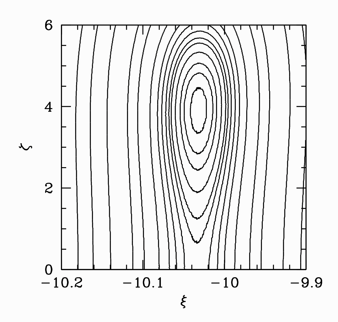
Figure 3: The contours show equipotentials in the $\eta=0$ plane for the case $\mu=0.001$ and $\beta=1.0008$. We see that there is a narrow libration region about this equilibrium point, potentially available to very small dust whose radiation pressure can outweight the gravity of the host star.

Although these equilibria exist in the Hill expansion version, they occur only close to the primary (as the radiating body) and, as such, are better described in the full restricted problem. We will revisit this question in § 4.1.

3 Periodic Orbits

Our principal goal is to understand the nature of long-lived dust particles orbiting a planet, such that they might be imaged in scattered light. In order to better understand this, we wish to understand the orbits that are stable around the planet, subject to the combined effects of gravity and radiation pressure. Henon (1969, 1970) presented a classic analysis of the different families of periodic orbits in the Hill problem. We wish to understand how the effects of radiation pressure change this. Before we do that, it is worth briefly reviewing the simply periodic orbit families as classified by Henon.

Families $a$ and $c$ represent the (unstable) extensions of the libration orbits about the Lagrange equilibria at $L_{1}$ and $L_{2}$. The families $g$ and $f$ represent the prograde and retrograde satellite orbits of the planetary body. The prograde orbit family splits, at critical point $g1$, with the introduction of a second orbital family $g^{\prime}$ (which contains both a stable and unstable equilibrium for some ranges of $C_{H}$). Family $g$ also becomes doubly periodic at a critical point $g2$.

3.1 Asymptotic Solutions

We can gain some preliminary insight into the influence of radiation pressure by considering the asymptotic limits of the periodic orbits in the limit $\Delta\rightarrow\infty$, so we are looking for simply periodic solutions to the equations

$$\ddot{\xi}-2\dot{\eta} = Q^{\prime}+\left(3-2\beta\right)\xi$$ (11)

$$\ddot{\eta}+2\dot{\xi} = \beta\eta$$ (12)

We will adopt a trial solution of $\xi=\xi_{0}+K_{1}\cos\omega t$ and $\eta=K_{2}\sin\omega t$ (assuming a judiciously chosen origin for time). Note that there is no term linear in $t$ as in Henon’s version, because of the $\beta\eta$ term on the right hand side of equation (12) and because the presence of the $Q^{\prime}$ term is sufficient to determine $\xi_{0}$ (which would require a contribution from the $\dot{\eta}$ term otherwise).

Inserting this trial solution into equations (11) and (12) implies a requirement on the frequency, namely

$$4\omega^{2}=\left(\omega^{2}+\beta\right)\left(\omega^{2}+3-2\beta\right)$$ (13)

which yields the solution

$$\omega^{2}=\frac{1}{2}\left[1+\beta\pm\left(1-10\beta+9\beta^{2}\right)^{1/2}\right]$$ (14)

For $\beta=0$, the solutions are either $\omega^{2}=0$ or $\omega^{2}=1$ (Henon’s solution). For finite $\beta$, we have real solutions for $\beta<\beta_{crit}=0.11095$. Larger values yield complex frequencies, suggesting that there are no stable asymptotic solutions for larger $\beta$. Figure 4 demonstrates the form of these solutions.

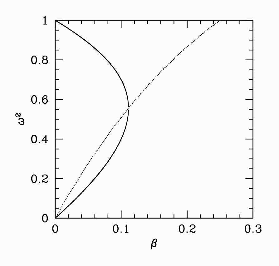
Figure 4: The solid curve indicates the roots of equation (14) for the asymptotic solution for $\mu=10^{-3}$. The dotted line represents the condition that the coefficient in front of $K_{1}$ in equation (15) remains positive (so that it still applies to the retrograde case). Thus, the branch of the solid curve above the dotted line corresponds to the standard asymptotic solution (which applies as $C_{H}\rightarrow-\infty$). The lower branch represents a second asymptotic solution, which applies in the limit $C_{H}\rightarrow\infty$.

3.1.1 The quasi-satellites

To complete the solution, $\xi_{0}=-Q^{\prime}/(3-2\beta)$. The expression for the constant, in this limit, is

$$C_{H}=-\frac{(Q^{\prime})^{2}}{3-2\beta}-\frac{\omega^{4}-\beta(3-2\beta)}{\omega^{2}+\beta}K_{1}^{2}$$ (15)

This recovers $C_{H}=-K_{1}^{2}$ in the $\beta\rightarrow 0$ limit, demonstrating that this is the asymptotic form of Henon’s family $f$. We note that the sign of the coefficient to $K_{1}$ in equation (15) changes when $\omega^{2}=2\beta(3-2\beta)/(1+\beta)$, which also happens to mark the maximum $\beta$ at which $\omega$ is real.

In the purely gravitational case, Henon showed that the retrograde family $f$ show stable equilibria in the asymptotic limit of large distances, and we now understand that these are associated with the class of orbits termed ‘quasi-satellites’ (Mikkola & Innanen, 1997; Wiegert et al., 2000; Giuppone et al., 2010). Our results demonstrate that the existence of this class of orbits is not universal under the influence of radiation pressure. For strong enough $\beta$ there is no longer such a stable asymptotic solution.

Furthermore, even for $\beta<\beta_{crit}$, we find two solutions for $\omega^{2}$. One applies in the limit $C_{H}\rightarrow-\infty$ (as occurs in the purely gravitational case), and the other in the limit $C_{H}\rightarrow+\infty$. This suggests that finite $\beta$ below the critical value should actually yield two equilibrium families at fixed $K_{1}$, rather than the single one in the $\beta=0$ limit. The solutions are given by

$$\xi = -\frac{Q^{\prime}}{3-2\beta}+K_{1}\cos\omega t$$ (16)

$$\eta = -\frac{2\omega}{\omega^{2}+\beta}K_{1}\sin\omega t$$ (17)

Thus, both solutions correspond to ellipses, although the amplitude in the $\eta$ direction will be different at the same $K_{1}$ (also corresponding to a different $C_{H}$).

This second asymptotic solution does not occur in the Photogravitational Hill problem (Markellos et al., 2000; Kanavos et al., 2002; Perdiou et al., 2012), where only the shift due to the $Q^{\prime}$ is introduced. However, stable orbits corresponding to this equilibrium can be observed in numerical orbital integrations of the full restricted three body problem with radiation (e.g. Zotos, 2015). As we shall see below, this solution may also have observational implications for the properties of the enigmatic object Fomalhaut b.

3.1.2 Orbits with Consecutive Collisions

Henon also discussed a class of solutions wherein the orbits exhibited excursions to arbitrarily large distances, but also returned periodically to $\xi=0$, $\eta=0$ to scatter off the secondary, terming these the “orbits with consecutive collisions”. These proved to be the asymptotic forms of the families $a$, $c$, $g$ and $g^{\prime}$. However, an integral part of these asymptotic solutions were terms that provided the $\eta$ component of the solution with either an additive constant or a term linear in time. As noted above, equation (12) no longer admits such solutions, and so we find no equivalents to these asymptotic solutions in this case.

3.2 Prograde Orbits

A more comprehensive survey of the simple periodic orbits requires direct numerical integration of the equations of motion (1),(2) and (3). Here we will restrict ourselves to the orbital plane, as the out-of-plane equilibria are too far from the planet to be realistically included in the Hill limit. We adopt a similar orbital classification procedure as discussed in Henon (1969). We begin integrations with $\eta=0$ and $\dot{\xi}=0$ and choose an initial value for $\xi$, and a value for $\dot{\eta}$ based on an assumed value of $C_{H}$. The positive sign of $\dot{\eta}$ is chosen and we record the $\xi$ and $\dot{\xi}$ every time the orbit crosses the $\eta=0$ plane moving in the positive direction. This is used to construct a Poincare plot. Equilibria are defined as those orbits for which $\xi$ does not change from the initial value on the first complete orbit (i.e. simple periodic orbits in the definition of Henon). The stability of each equilibrium is evaluated by constructing the linear mapping of orbits surrounding the equilibrium and evaluating the eigenvalues of the resulting matrix (Tremaine, 2023). We map out the families of simply periodic orbits and will also describe a subset of the doubly periodic orbits which can impact the stability of some of the simply periodic families.

Figure 5 shows the resulting prograde equilibria, for the mass ratio $\mu=10^{-3}$. In the upper panel, the red curves represent the original orbital families for $\beta=0$ from Henon (1969). The black curves show the case for weak radiation pressure ($\beta=0.001$, so $Q=0.02$). The red curves show the original Henon orbit families of $g$ and $g^{\prime}$ (and the unstable family $a$). In the case of $\beta=0$, the appearance of family $g^{\prime}$ occurs at $C_{H}=4.4999$ and $\xi_{0}=0.2835$ and all three equilibria move away from this point as $C_{H}$ decreases. In the case of non-zero $\beta$ we find that, instead of a point of intersection, the new family $G^{\prime}$ emerges at lower values of $\xi$ than the equilibrium on the $G$ family at the corresponding $C_{H}$. The evolution, in this case, is more akin to an avoided crossing of two families, $G$ and $G^{\prime}$, each of which contains a portion of the original $g$ and $g^{\prime}$. A similar behaviour occurs in the prior definition of the photogravitational Hill problem (Markellos et al., 2000; Kanavos et al., 2002), albeit with different $G$ and $G^{\prime}$ (corresponding to linking different combinations of the sections of $g$ and $g^{\prime}$). In our case, the family $G$ extends from high $C_{H}$ all the way to the Lagrange point, with the equilibria distorting from quasi-circular shapes (deep in the potential well) to more elongated shapes as they approach the Lagrange point. The family $G^{\prime}$, on the other hand, only exists at moderate $C_{H}$, linking a stable branch of compact eccentric orbits to the unstable branch that was originally the extension of the g family.

The blue curves in the upper panel of Figure 5 show the equilibria for the case of $\beta=0.01$. The $G$ family shifts to larger $C_{H}$ at fixed $\xi$, while the $G^{\prime}$ family shifts to the left (lower $C_{H}$ at fixed $\xi$). Note also that the $A$ family (the analog of the $a$ family) shifts down (to lower $\xi$ at fixed $C_{H}$), so that the $A$ and $G^{\prime}$ families start to approach each other as $\beta$ increases. The lower panel of Figure 5 shows the evolution of the orbital families as $\beta$ increases. The magenta curves show the case of $\beta=0.05$. As the radiation pressure grows, the forbidden region moves to large $C_{H}$ and $G$ family shifts in the same direction. Conversely, the $G^{\prime}$ family shifts down to lower $C_{H}$. The black curves show the case for $\beta=0.1$. In this case, the family $G^{\prime}$ no longer exists.

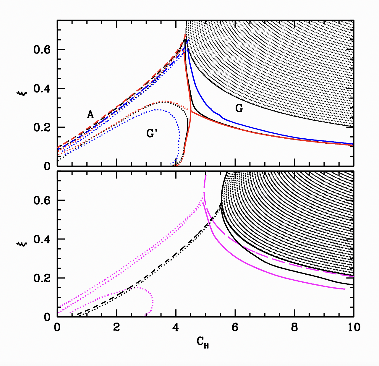
Figure 5: The dark shaded region indicates the region in which orbits are disallowed. In the upper panel this is shown for $\beta=0$. The red curves show the prograde equilibrium orbit families for the case $\beta=0$. The black curves show how these shift once a small radiation pressure ($\beta=0.001$, $Q^{\prime}=0.02$) is included. The blue curve shows the case for $\beta=0.01$ ($Q^{\prime}=0.2$). In the lower panel, the magenta curves show the case for $\beta=0.05$ and the black curves show the case for $\beta=0.1$. The shaded forbidden region shown here is for $\beta=0.1$ and the magenta long dashed line shows the boundary of the forbidden region in the case $\beta=0.05$. In both panels, the solid lines indicate those equilibria that are stable, and the dotted lines indicate the unstable portions of the $G/G^{\prime}$ families. The dashed lines indicate the unstable $A$ family.

In the case of $\beta=0$, the association of the two branches of the $g^{\prime}$ family are natural, as their orbit shapes are the same except for a simple rotation of 180^∘ about the $\eta$ axis. Once $\beta>0$, the symmetry of the potential is broken and the equivalent solutions are no longer as similar in shape. Indeed, it is now the two solutions of the $G^{\prime}$ branch that retain similar shape (initially, since one is unstable). Figure 6 shows the comparison of the equilibria for $C_{H}=4.4$ in both the $\beta=0$ and $\beta=10^{-3}$ cases.

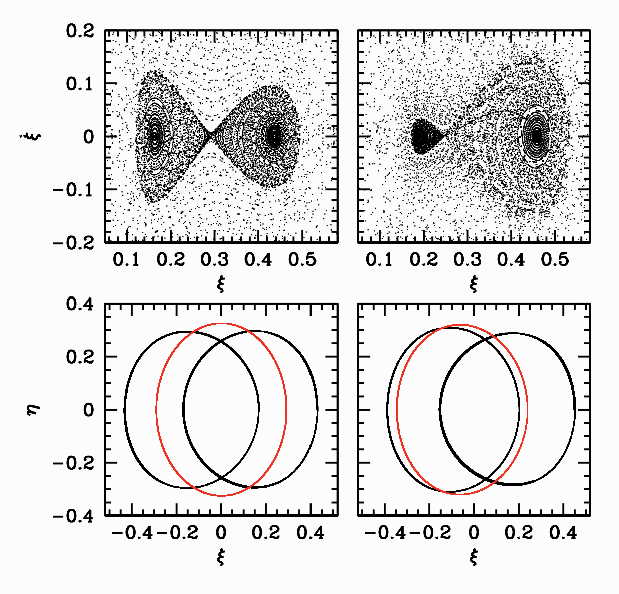
Figure 6: The two panels on the left are for the case of $\beta=0$ and the two panels on the right are for $\beta=10^{-3}$. All integrations are for the case $C_{H}=4.4$. In the upper panels we show the Poincare plots. Each shows two clear stable equilibria and one saddle point between them. However, the $\beta=0$ case is much more symmetric. The differences can also be seen in the lower panels, which show the orbits corresponding to the equilibria (red is unstable in the long term). On the left, the two stable equilibria are close to reflection-symmetric in $\xi$, but the plot on the right shows that this symmetry has been broken by the presence of radiation pressure. It is now the two $G^{\prime}$ solutions that share a similar shape – because they emerge together as $C_{H}$ drops below the critical value.

The $G$ family solution continues to evolve to ever more eccentric shapes as $C_{H}$ decreases. As $C_{H}$ decreases, the shape of the inner stable solution on the $G^{\prime}$ branch also evolves to a more eccentric shape and approaches the same dichotomy with the $G$ solution as in the $\beta=0$ case. Figure 7 shows the case for $C_{H}=4.3$. We see that the two equilibria are now islands of stability with an intervening unstable region, and that the remaining stable equilibria are now more similar (and more eccentric).

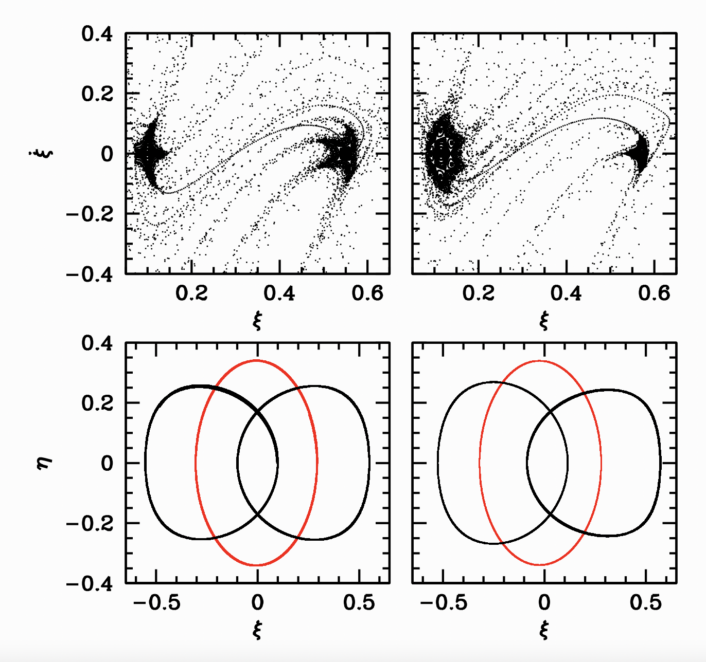
Figure 7: The two panels on the left are for the case of $\beta=0$ and the two panels on the right are for $\beta=10^{-3}$. All integrations are for the case $C_{H}=4.3$. In the upper panels we show the Poincare plots. Each again shows two clear stable equilibria and one saddle point between them. The lower panels show the orbits corresponding to the equilibria in each case. The comparison between the two lower panels shows that the shapes of the $G$ and $G^{\prime}$ orbits evolve towards similar shapes as $C_{H}$ drops, approaching a similar structure as the original $\beta=0$ case.

As $\beta$ increases, the gap in $C_{H}$ between the $G$ and $G^{\prime}$ families increases, and the $G^{\prime}$ family eventually becomes completely unstable for $\beta>0.01$. For $\beta>0.095$, the $G^{\prime}$ family of equilibria disappears.

3.3 Retrograde Orbits

A striking feature of Henon’s original analysis was that the family $f$ of retrograde simply periodic orbits remained stable to arbitrarily large distances from the planet, merging into the class of orbits referred to as quasi-satellites. Figure 8 shows how this family adjusts to the strength of the radiation pressure.

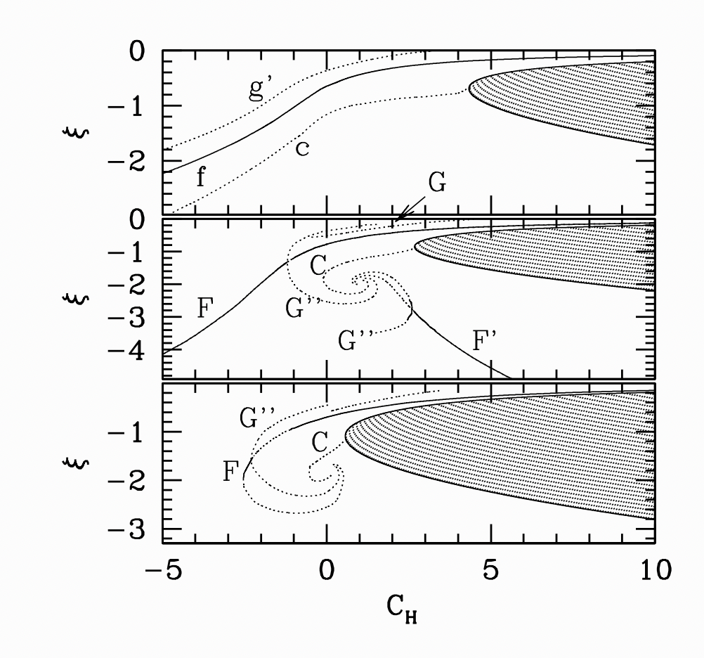
Figure 8: The upper panel shows the retrograde orbital families in the original $\beta=0$ case. The black solid curve shows the original stable family and the black dotted curves shows the unstable equilibrium family $c$ and the negative intersection of the $g^{\prime}$ family. The middle panel shows the orbital families for the case $\beta=0.1$. The family $F$ is the equivalent of $f$ and is also stable except for a brief crossing with the unstable $G^{\prime\prime}$ family. We also find the family $F^{\prime}$, associated with the second asymptotic solution, and which is also stable at large enough distances. The shapes of the unstable families $C$,$G$ and $G^{\prime\prime}$ are affected by the presence of the triangular equilibria, as discussed in the appendix. The bottom panel shows the case for $\beta=0.2$. We see here that the family $F$ no longer continues to arbitary distances. In all panels, the shaded region represents the forbidden region for that particular $\beta$.

For small values of $\beta$ the nature of the retrograde family (called $F$ here) remains similar to the $\beta=0$ case. However, for $\beta=0.1$, the curve shifts to larger separations more quickly, and begins to exhibit qualitatively new features for $\beta=0.2$. In the $\beta=0.2$ case, the $F$ family does not extend all the way to arbitrarily small $C_{H}$ but loops back to larger $C_{H}$ at larger $\left|\xi\right|$, forming an unstable branch. Figure 19 in Appendix A demonstrates this evolution.

The middle panel of Figure 8 also shows a solution branch, called $F^{\prime}$, which corresponds to the second asymptotic solution discussed in § 3. At large distances, this forms a second stable branch, shown as the blue curves in Figure 19 in the appendix. The co-existence of these two stable branches, $F$ and $F^{\prime}$ is shown in Figure 9 for the value $C_{H}=4$ and $\beta=0.1$.

Another striking feature of these equilibria is that there appears a ‘vortex-like’ feature around $C_{H}\sim 1$ and $\xi\sim-1.9$, where several different equilibrium curves converge. As discussed in Appendix A, and Figure 22, this appears to be the result of the interaction of the orbits with the triangular equilibrium points.

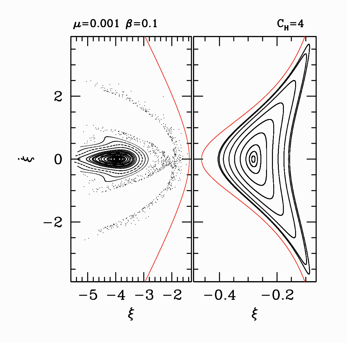
Figure 9: The two panels show the Poincare plot for the retrograde orbits in the case $\mu=10^{-3}$, $\beta=0.1$ and $C_{H}=4$. The red curves delineate the edges of the forbidden region, which separates the $F$ region of stability (on the right) from the $F^{\prime}$ region (on the left). In the left panel, the diffuse band of points near the red contour correspond to the quasi-circular orbits about the primary in the full restricted three-body problem. This is a diffuse band because these do not correspond to a fixed point family in the Hill problem.

We also show the evolution of the $G$ orbits (equivalent to the $g^{\prime}$ from Henon (1969)). These result from the part of the $G$ family that becomes doubly periodic, where the condition that the path cross the $\eta=0$ axis in the positive direction is satisfied for both positive and negative $\xi$. Thus, these curves form a pair with curves in the prograde case (Figure 5). In addition, we find another family of orbits, dubbed $G^{\prime\prime}$, which is also doubly periodic, but both crossings of the $\eta=0$ axis occur at $\xi<0$. These orbital families are outlined in Figure 16 and Figure 20 respectively.

Finally, we note that the $F$ and $F^{\prime}$ families are the only ones that extend to large distances for $\beta=0.1$, namely that $C$ and the $G$, $G^{\prime\prime}$ families have only a finite extent. This is consistent with the absence of any corresponding asymptotic solutions (§ 3.1.2).

3.4 Available Stable orbits

Our goal here is to determine the parameter space available for stable orbits under the influence of both planetary gravity and stellar radiation pressure. The interest in the simply periodic orbits is that stable regions are expected to surround these orbits, so that they form the ‘scaffolding’ around which the structure of long-term stable orbits is built.

Thus, we have performed a survey of all orbits specified by a choice of $\xi_{0}$ and $C_{H}$, with $\eta=0$ and $\dot{\xi}=0$, characterising their outcomes as to whether they remain within $\Delta=10$ of the planetary body after time=200 (where the period of the planetary orbit is 2$\pi$). Figure 10 shows the outcomes of this parameter scan for $\mu=0.001$ and three choices of $\beta=0$, $\beta=0.1$ and $\beta=0.2$.

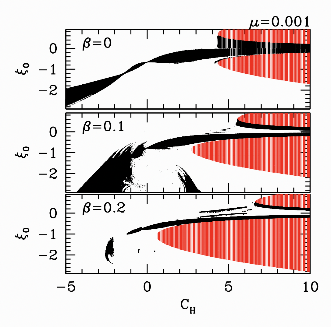
Figure 10: In each panel the red region is the range of forbidden orbits. Black points indicate initial conditions that produce orbits which remain within $\Delta=10$ after $t=200$ and so are considered stable. The strength of the radiation pressure increases from the top ($\beta=0$) to the botton ($\beta=0.2$). We see that the radiation pressure initially increases the range of stable distance orbits (see middle panel) but eventually truncates the stable branch of retrograde orbits (lower panel).

The $\beta=0$ case closely resembles Figure 12 of Henon (1970), demonstrating the existence of stable orbits, both prograde and retrograde, for $C_{H}>4.27$, and an extension of the stable retrograde family to arbitrarily large distances (this family is characterised as the quasisatellites). The middle panel of Figure 10 shows the case of moderate radiation pressure ($\beta=0.1$). We see that the prograde and retrograde stable regions at larger $C_{H}$ are now separated by a region where the orbits are unstable. This is mostly the consequence of orbits getting excited to essentially radial orbits and hitting the planet (Burns et al., 1979; Hamilton & Krivov, 1996; Zotos, 2015). The retrograde family still extends to larger radii and actually broadens, along with the presence of a second family of stable orbits at larger radii and positive $C_{H}$. This represents the second family of asymptotic solutions, $F^{\prime}$. Much of the other structure observed in Figure 8 does not appear in these figures because those additional equilibria are unstable. However, the $F^{\prime}$ family is robust and also appears in the full restricted three-body problem with radiation (as can be seen from Figure 10 of Zotos (2015), for example – albeit for the $\mu=0.5$ case).

Finally, the lower panel shows the case of strong radiation pressure $\beta=0.2$. Inside the Hill sphere the prograde and retrograde stable regions are again separated by a large region of mixed stable and unstable orbits. The retrograde family also does not now extend to arbitrarily large distances, as expected based on our asymptotic solutions.

3.5 Mass Dependance

Our discussion thus far has focussed on the case of a mass ratio $\mu=10^{-3}$, appropriate for a Jupiter-mass planet orbiting a Solar mass star. However, as we noted in our original derivation, our desire to retain the effects of non-infinitesimal $\beta$ means that our equations are not scale free as in the case of the original Hill problem. Thus, we must investigate the effect of mass.

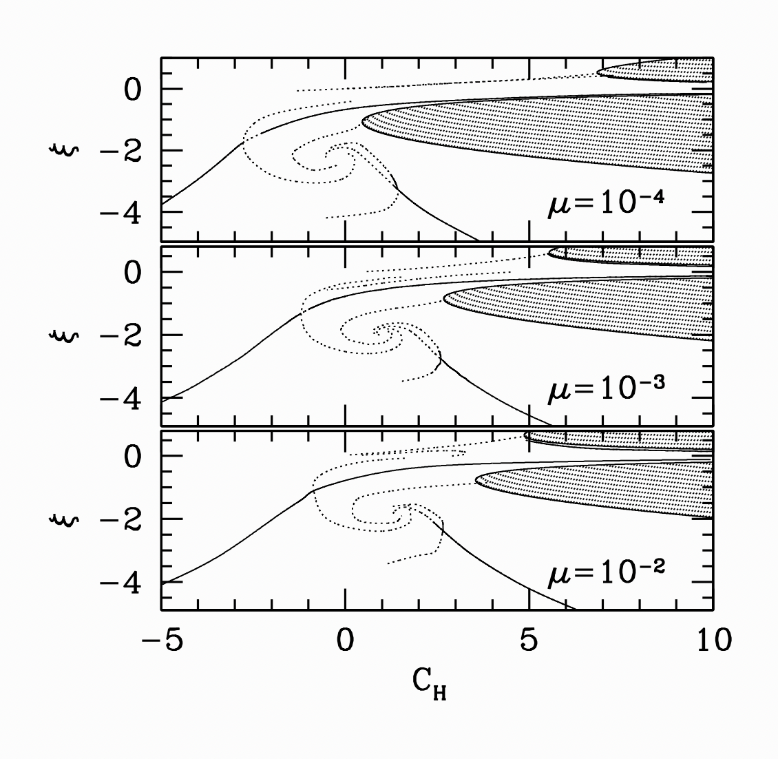
Figure 11: All three panels show the orbital families for the case $\beta=0.1$. In the upper panel, the secondary is only $\mu=10^{-4}$ of the total system mass. In the middle panel, $\mu=10^{-3}$ (so this is equivalent to the middle panel of Figure 8). In the lower panel the mass ratio is $\mu=0.01$. Once again, stable equilibria are maked by solid lines and unstable equilibria are marked by dotted lines.

Fortunately, most of the structure in the solutions is determined by the $\beta$ parameter itself, and the role of $\mu$ is primarily to determine a shift along the $\xi$ axis, through the effect of the $Q^{\prime}$ parameter. This is demonstrated in Figure 11, which shows the orbit families for the case of $\beta=0.1$ and three different mass ratios ($\mu=10^{-4}$, $\mu=10^{-3}$ and $\mu=10^{-2}$). We see that most of the structure is maintained, but that the lower mass families are shifted to lower $C_{H}$. If we examine the asymptotic solutions, we note that the frequencies $\omega$ depend only on $\beta$, not $Q^{\prime}$, and so the existence of the asymptotes should be independent of $\mu$.

At the higher mass ratio, there are some differences in the details, as the $G^{\prime}$ prograde family returns, even for $\beta=0.1$.

4 The full restricted three body problem

Our ultimate goal is to address potential observable signatures of a population of dust particles orbiting near the planet around which they are generated. We have identified the orbital families and stable regions as a function of radiation pressure. If we wish to observe structures associated with these orbital families, we need to map the Hill sphere results to the full three body problem, since it is in this frame that observations will be made. Thus, we have repeated the calculation from the previous section in the full restricted three body problem, with radiation. We once again choose initial conditions with $\xi_{0}$, $\eta=\zeta=0$, $\dot{\xi}=\dot{\zeta}=0$ and $\dot{\eta}$ chosen from $C_{H}$. We then integrate the orbits using the full equations of motion. We also apply a random offset in the starting time (ranging over a full planetary orbital period) to avoid any artificial relative phases between different trajectories.

Figure 12 shows the positions of the test particles that remain near the planet after $t=200$. We have plotted this in the reference from of the full reduced three body problem (so that $X=1-\mu+\mu^{1/3}\xi$ and $Y=\mu^{1/3}\eta$. We show three panels, for $\beta=0$ (left panel), $\beta=0.1$ (middle panel) and $\beta=0.2$ (right panel). The location of the planet is given by the solid red point, and circles of 1.0 and 0.5 Hill radii are shown.

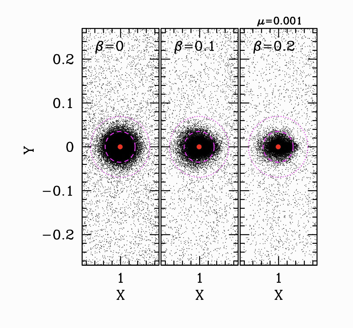
Figure 12: Each black point plotted represents the position of a particle, released in the Hill sphere, after $T=200$. In the left panel, we assume no radiation pressure ($\beta=0$). The red point indicate the position of the planet and the magenta curves represent the Hill radius (dotted line) and 0.5 Hill radii (dashed line). In the middle panel, the particles experience radiation pressure with $\beta=0.1$ and, in the right hand panel $\beta=0.2$. These are all for the case $\mu=0.001$.

In the purely gravitational case ($\beta=0$), the distribution of long-lived points near the planet is approximately circular, and confined within $\sim 0.4$ Hill radii, as expected based on prior work in this problem (Hunter, 1967; Domingos et al., 2006). As the radiation pressure gets stronger, the shape of the stable population becomes elongated along the $X$ axis, with the width shrinking in the Y direction. This is a consequence of the distortion of the stable orbits as seen in the various galleries in Appendix A. We will discuss the observational signatures of this in § 5.

4.1 The Out-of-Plane Equilibria

If radiation pressure is very strong ($\beta>1$), then the net force from the primary becomes outwardly directed, and the balance between this force and the gravitational pull of the secondary can provide the force balance to produce new, out-of-plane equilibria (Schuerman, 1980; Simmons et al., 1985), as discussed in § 2.2. As we noted before, the locations of these equilibria are too far from the planet to be realistically treated in the Hill problem. However, the qualitative features discussed in § 2.2 still remain in the full retricted three-body problem. Figure 13 shows the location of the $L_{6}$ equilibrium point in the $y=0$ plane as a function of $\beta-1$. There is an equivalent mirror-image $L_{7}$ point located below the orbital plane.

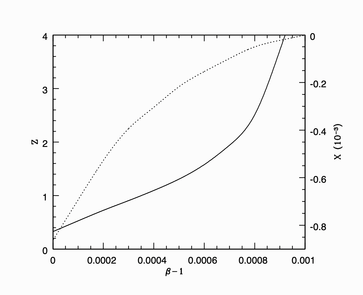
Figure 13: The solid curve shows the location of the $z$ coordinate of the $L_{6}$ equilibrium point as a function of $\beta$. The dotted curve shows the equivalent $x$ coordinate (these both lie in the y=0 plane). This is for the case $\mu=0.001$.

These equilibria are very far removed from the assumed source of dust generation in this model, but may potentially affect the evolution of any dust that manages to reach this point. However, these are not suitable locations for the long-term trapping of dust because the equilibria are unstable (Simmons et al., 1985).

5 Observational Signatures

The direct observation of a self-luminous exoplanet requires the detection of an unresolved point source, usually at the infrared wavelengths where self-powered emission is expected to peak. However, if there is a substantial population of circumplanetary dust, the scattering of stellar light by the dust may provide an observable signature at shorter wavelengths more characteristic of the stellar emission. Similarly, with a large enough surface area, the thermal emission from the dust may overwhelm that of the planet, although this is a function of wavelength (Kennedy & Wyatt, 2011). Furthermore, such populations are more extended and thus potentially resolvable.

5.1 The shape of a trapped dust population

To model the potential signature of a circumplanetary dust population, we evolve forward three-dimensional trajectories of particles initially drawn from a singular isothermal sphere radius distribution, spherically distributed except that we exclude starting positions with inclinations between $60^{\circ}$–$130^{\circ}$ of the orbital plane. This is based on the assumption that the dust initial distribution should follow that of the parent bodies. The observed irregular satellites in the Solar system show this deficit (Jewitt & Haghighipour, 2007), which is believed to be a consequence of the dynamical instability of such orbits (Hamilton & Burns, 1991; Nesvorný et al., 2003).

Figure 14 shows contour plots of the density of particles for the cases $\beta=0.1$ (left panels) and $\beta=0.2$ (right panels), in both the X-Y plane (at Z=0) and in the X-Z plane (at Y=0). The distribution of particles is primarily confined within the seperatrices that pass through $L_{2}$ and it is this surface which is responsible for the elongation of the observed distribution. The half-max and quarter-max contours are marked in red, demonstrating this elongation, in both the X-Y and X-Z planes.

If we characterise the shape of the original parent population, by following the above model with $\beta=0$, we find that the Full-Width Half Max (FWHM) of the surviving particles is $0.28$ of the Hill diameter in the X direction, $0.27$ in the $Y$ direction, and 0.20 in the $Z$ direction. These proportions increase to 0.39, 0.37 and 0.30 respectively, if we take the widths at quarter of the maximum (FWQM). Thus, the underlying population is spherically symmetric in projection, despite the Kozai-induced holes at the pole.

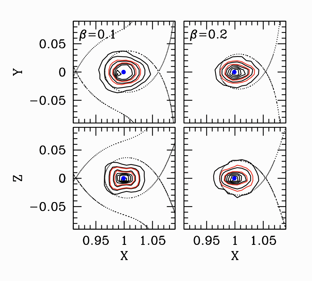
Figure 14: The contours represent surface density of points for particles orbiting about a secondary with mass ratio $\mu=10^{-3}$ and radiation pressure $\beta=0.1$ (left panels) and $\beta=0.2$ (right panels). The blue solid point represents the position of the secondary. The red solid contours represent the value corresponding to half the maximum and a value a quarter of the maximum. The dotted contours represents the equipotential that pass through the $L_{1}$ and $L_{2}$ points. It is the confinement within the $L_{2}$ contour that is responsible for the elongated shape of the distribution. The upper panel represents the X-Y plane, and the lower panel the X-Z plane.

The results of the $\beta=0.1$ integration show FWHM of 0.30 in the $X$ direction, 0.24 in the $Y$ direction and $0.20$ in the $Z$ direction (with 0.40, 0.31 and 0.29 at FWQM). Thus, the distribution of surviving dust is flattened with an aspect ratio $\sim 1.3:1$. For $\beta=0.2$ the flattening becomes even more extreme, with FWHM of $0.31$ in $X$, 0.21 in $Y$ and 0.17 in $Z$ (with 0.43, 0.29 and 0.33 respectively at FWQM). Thus, the elongation of the dust population increases with increasing $\beta$.

This suggests a potential signature of the influence of radiation pressure – the observation of an extended distribution of dust yields a potentially resolvable target in thermal or scattered emission, and one that should become more elongated as one approaches shorter wavelengths that probe smaller particles and larger $\beta$.

5.2 Fomalhaut: A case study

Although the above model can be applied to any star/planet system imaged in scattered or thermal light, the star Fomalhaut and its attendant dust structures offers the most complete application to date. The narrow dust ring imaged by Kalas et al. (2005) has long stimulated discussion about the origin of this dust and how planets might sculpt it (Quillen, 2006; Chiang et al., 2009), and the detection of a candidate planet Fomalhaut b (Kalas et al., 2008; Kalas et al., 2013) has further amplified this discussion, including alternative interpretations (Currie et al., 2012).

The narrowness of the dust ring is another feature that needs explanation. Hayakawa & Hansen (2023) offer an alternative to the standard birth ring of planetesimals –possibly sculpted by additional planets (Boley et al., 2012), in which the dust is generated in a circumplanetary cloud of irregular satellites and then spirals out through the $L_{2}$ point, sherpherded into a thin ring by the restrictions imposed by the relevant Jacobi constant. The discussion of Hayakawa & Hansen (2023) focusses on the ring morphology, but the potential observability of the dust bound to the planet is a further interesting consideration. Kennedy & Wyatt (2011) discuss the application of this model to the observations of Fomalhaut b, but can be considered relevant to any putative irregular satellite cloud, either at the location of Fomalhaut b or elsewhere in the system.

Kennedy & Wyatt (2011) discuss a dust cloud whose spatial distribution follows that of the parent bodies, but our calculations above show that the dust dynamics under the influence of radiation pressure result in an elongated structure, with the long axis pointing along the star–planet line. Interestingly, such a signature was discussed by Kalas et al. (2013) for Fomalhaut b, although it could not be discounted that this was a residual signature of speckle noise.

An additional signature of the Hayakawa & Hansen (2023) model is that the planet should lie slightly interior to the inner edge of the dust ring, by virtue of the geometry of the equipotential that passes through the $L_{2}$ point (through which the unbound dust escapes). This implies that the planet should lie at $\sim 0.92$ the semi-major axis as measured by the shape of the ring. Once again, Fomalhaut b lies at about the correct distance from the ring, although the proper motion of the planet does not conform to this model any more than it does for the gravitational sculpting model of Quillen (2006); Chiang et al. (2009).

5.2.1 Fom b as a quasi-satellite?

.

The fading and eventual disappearance of Fomalhaut b (Kalas et al., 2013; Gaspar & Rieke, 2020) in the optical suggests that this object is not a planet but a dust cloud undergoing dispersal over a timescale of decades. The origin of the dust cloud has been postulated to be the result of a collision between planetesimals (Currie et al., 2012; Kalas et al., 2013; Gaspar & Rieke, 2020) although the origin of the parent population is still somewhat in question (since it is not located in the nominal birth ring associated with the dust disk). The discovery of interior belts (Gáspár et al., 2023) is a possible source, although the path from the quasi-circular interior belts to a coherent, highly elliptical, dispersing orbit has yet to be described in detail.

The population of quasi-satellites associated with Henon’s $f$ family offers a potential parent population. If the planet associated with the dust disk is accompanied by a population of planetesimals in quasi-satellite orbits, then these objects would have heliocentric orbits with semi-major axes within $\sim 20\%$ of the planetary orbit, and with eccentricities $\sim 0.1$–$0.3$. However, if such an object were to release dust that is subject to radiation pressure, the orbit of the dust would deviate from that of the parent body, because the $F$ and $F^{\prime}$ orbits in Figures 8 and 10 are not the same as for the $\beta=0$ case. Indeed, the inferred heliocentric parameters for particles on these orbits can deviate substantially from those characteristic of the planet itself, even reaching apparently unbound values for part of the orbit (see appendix B for an example).

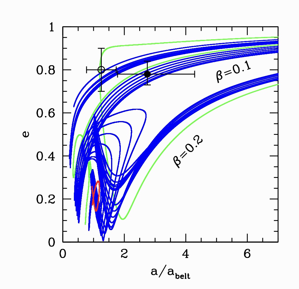
Figure 15: The solid point shows the estimated orbital parameters of Fom b from Gaspar & Rieke (2020), while the open point represents the earlier measurement of Kalas et al. (2013). The red curve shows the evolution of the heliocentric parameters of quasi-satellite of a Jupiter-mass planet orbiting at the distance of the primary Fomalhaut dust belt. The blue curve shows the orbital evolution if we start with the same initial conditions as the red curve, but assume radiation pressure with $\beta=0.1$. The green curve corresponds to $\beta=0.2$.

Figure 15 demonstrates how radiation pressure would cause the dust to deviate. The red trajectory shows the variation in semi-major axis (scaled relative to the parent planet) and eccentricity of a quasi-satellite trajectory in the case $\beta=0$. If one takes the same initial position and velocity, but calculates the trajectory with $\beta=0.1$ (blue curve) and $\beta=0.2$ (green curve), one finds that the dust makes several loops in semi-major axis and eccentricity, which pass through the region occupied by the measured orbital parameters of Fomalhaut b. For $\beta=0.2$, the dust does pass through the observed region of parameter space, but is ejected pretty quickly. However, for $\beta=0.1$, the orbit lies within the stable part associated with the $F^{\prime}$ family, and makes repeated passages through the observed region. These results suggest that the dust involved in the cloud should have $\beta\sim 0.1$ to increase the chances of observation. For values close to $\beta\sim 0$, the orbital parameters do not approach those observed, and for $\beta\sim 0.2$, the dust leaves the system rapidly.

If Fom b is a dissipating dust cloud, the rate at which such objects are generated is very uncertain. The fact that one has been observed over the course of our brief observations suggest that the rate is non-negligible (or we have been very lucky). Although it may be challenging to justify a high rate of collision in the system, we should note that the Solar system contains populations of ‘active asteroids’ that need not experience collisions to eject dust (e.g. Jewitt, 2012). If more such dust clouds are discovered in the future, their kinematics should be similar to that described in Figure 15 in this model, whereas they should exhibit a much wider range of parameters if they are being seeded by the interior belts observed in the system.

5.2.2 Fom b as an $L_{6}$ point?

Much has been made of the curious orbit that Fom b appears to trace. Most of the attempted physical explanations assume an orbit close to coplanar with the disk. If we were to hypothesize that this feature was, instead, associated with the out-of-plane equilibria due to radiation pressure, could this very different geometry provide a better explanation for Fom b? The short answer is no. One can plot the locus of possible positions of the $L_{6}$ and $L_{7}$ points, assuming that the Fomalhaut ring indicates the orbital plane for any secondary. For different values of $\beta$, these points lie at different heights above the plane which, in turn, project to different locations on the sky plane. However, none of them come close to Fomalhaut b.

Somewhat more strikingly, the resulting locus does pass close to the location of the feature dubbed the ‘Great Dust Cloud’ in the JWST images of this system (Gáspár et al., 2023). However, it requires very small particles to achieve $\beta>1$, and so the 23.5 $\mu$m bandpass seems like an unlikely wavelength to identify such features. Furthermore, ground-based imaging suggests this feature may be a background feature (Kennedy et al., 2023) and so this agreement appears to be a coincidence.

5.2.3 Searching for the True Planet

We have thus far focussed on the potential shape of a population of trapped dust. To estimate the brightness, we must account for the finite lifetime of dust trapped within the Hill sphere, subject to both erosion due to collisional evolution, and to the loss of material through the $L_{2}$ point to the thin disk. In Hayakawa & Hansen (2023) we estimated the average time for escape to be $\sim 10^{7}$ years for grains with $\beta\sim$ 0.1–0.2 in orbit around a Jupiter mass planet at 140 AU. In similar fashion as Kennedy & Wyatt (2011), we can estimate the collisional timescale in a population of irregular satellites to be

$$T_{coll}\sim 4\,{\rm Myr}\left(\frac{a}{140AU}\right)^{\frac{7}{2}}\left(\frac{s}{10\mu m}\right)\left(\frac{M_{p}}{1M_{J}}\right)^{\frac{2}{3}}\left(\frac{M_{irr}}{M_{\leftmoon}}\right)^{-1}$$ (18)

assuming a total mass $M_{irr}$ of order a Lunar mass, confined to a volume $\sim 0.3$ Hill radii. We truncate the collisional cascade at dust sizes $\sim 10\mu$m, because $\beta\sim 0.18(10\mu m/s)$ for the Fomalhaut system and this is approximately the $\beta$ value where dust escapes before being ground down further (Hayakawa & Hansen, 2023). Thus, an irregular satellite cloud of this size would be in approximate steady state. We note that this age is younger than the overall age of the Fomalhaut system, but we expect irregular satellites to be captured during three-body interactions during epochs of dynamical instability in a planetary system, which can occur at ages of hundreds of millions of years (as has been hypothesized in our own Solar system).

In a collisional cascade, the mass and collision rate is dominated by the most massive bodies, but the surface area for emission and scattering is dominated by the smaller bodies. Assuming a Dohnanyi (1969) power law, extending down from 100 km to 10$\mu$m, we estimate a total surface area $\sim 5\times 10^{22}cm^{2}$ (roughly a factor of 3 smaller than that estimated by Kennedy & Wyatt (2011) for this system with slightly different assumptions).

To assess whether this is observable in the recent JWST images (Gáspár et al., 2023), we estimate that the dust should be at a temperature $\sim 47{\rm K}\left(a/140AU\right)^{-1/2}$. At 23$\mu$m, and at a distance of 7.7 pc, this implies an object with total observable flux $\sim 0.4\mu$Jy, or $\sim 1\mu$Jy per square arcsecond, if spread over an angular width of $\sim 0.4^{\prime\prime}$ (corresponding to 0.3 Hill radii). This is $\sim 150$ times fainter than the ‘Great Dust Cloud’ and about ten times fainter than the $1\sigma$ noise level estimated by Gáspár et al. (2023).

The above estimate assumes a blind search, but one might also help to narrow the field if one associates the Fom b orbit with an associated quasi-satellite. However, quasi-satellites can exhibit large excursions relative to their guiding center planets, so the identification of Fom b with such a population does not narrow the location of any particular planet (other than locating it in the western half of the orbit).

We conclude that the nominal model is not yet easily detectable with the extant JWST data, but does lie within an order of magnitude of the current noise levels. Thus, either deeper observations or a more optimistic estimate for the size of the dust population could bring observations and theory into comparable brightness levels.

6 Conclusions

The calculations in this paper represent a follow-on from the calculations of Hayakawa & Hansen (2023). In particular, if we posit that geometrically thin dust rings are the product of the grinding down of an irregular satellite population trapped within the Hill sphere of an extrasolar planet, then we seek to identify observational signatures of a dust population that remains bound to the planet.

To that end, we have studied the orbital properties of dust affected by radiation pressure and the gravity of the secondary body, and classified the kinds of periodic solutions that may occur. In particular, we have extended our study to values of $\beta$ that exceed the infinitesimal limit treated in many previous studies. We find that the orbital families of the $\beta=0$ case are reproduced for small $\beta$ but some of them disappear or are substantially modified at larger values of $\beta$. In particular, we find a second stable asymptotic family of retrograde solutions for moderate $\beta$.

The modified orbital properties suggest that a bound dust cloud should be elongated along the primary–secondary axis, with the level of elongation increasing with $\beta$. This suggests that resolved sources whose shapes change with the observed wavelength may be the signature of radiation pressure at work.

As an application of our model we consider the Fomalhaut system and its enigmatic planet/dust cloud Fomalhaut b. We find that the curious orbital properties of Fom b could be explained if the parent body of the dust cloud was following a quasi-satellite trajectory relative to a yet-undiscovered planet orbiting in the narrow dust disk. The effect of radiation pressure on dust released from such bodies can produce orbital elements consistent with those observed.

Data availability: The data underlying this article will be shared on reasonable request to the corresponding author.

This research was supported by NASA grant 80NSSC20K0266. This research has made use of NASA’s Astrophysics Data System Bibliographic Services.

Appendix A A: Orbit Gallery

The primary family of stable prograde orbits in Henon’s analysis is $g$, intersecting with a secondary family $g^{\prime}$ that emerges below a critical value of $C_{H}$. The equivalent families $G$ and $G^{\prime}$ for non-zero $\beta$ do not map directly onto $g$ and $g^{\prime}$ because they do not intersect.

Figure 16 shows the generalisation $G$ of this family ($g$) for $\mu=0.001$ and $\beta=0.001$ (black), $\beta=0.05$ (red) and $\beta=0.1$ (blue). Each panel is chosen to have the same $\xi(0)$, which means that the $C_{H}$ will be different for different $\beta$. The progression from the upper left to bottom right follows the decrease of $C_{H}$ (for fixed $\beta$). The principal qualitative effect of increasing $\beta$ is compression of the orbit shape in the $\eta$ direction, i.e. the effect of radiation pressure is to elongate the orbit along the primary–secondary axis.

We have designated this family as $G$ because we wish to use this for the main family of stable prograde orbits. However, the comparison with Figure 16 and the corresponding Figures 4, 5 and 6 of Henon (1969) shows that the orbits for lower $C_{H}$ represent the generalisation of $g^{\prime}$ rather than $g$. Note also that, in the lower two panels, the solutions are double periodic and include an intersection moving in the positive direction at $\xi<0$. These are the origin of the $G$ curves in Figure 8.

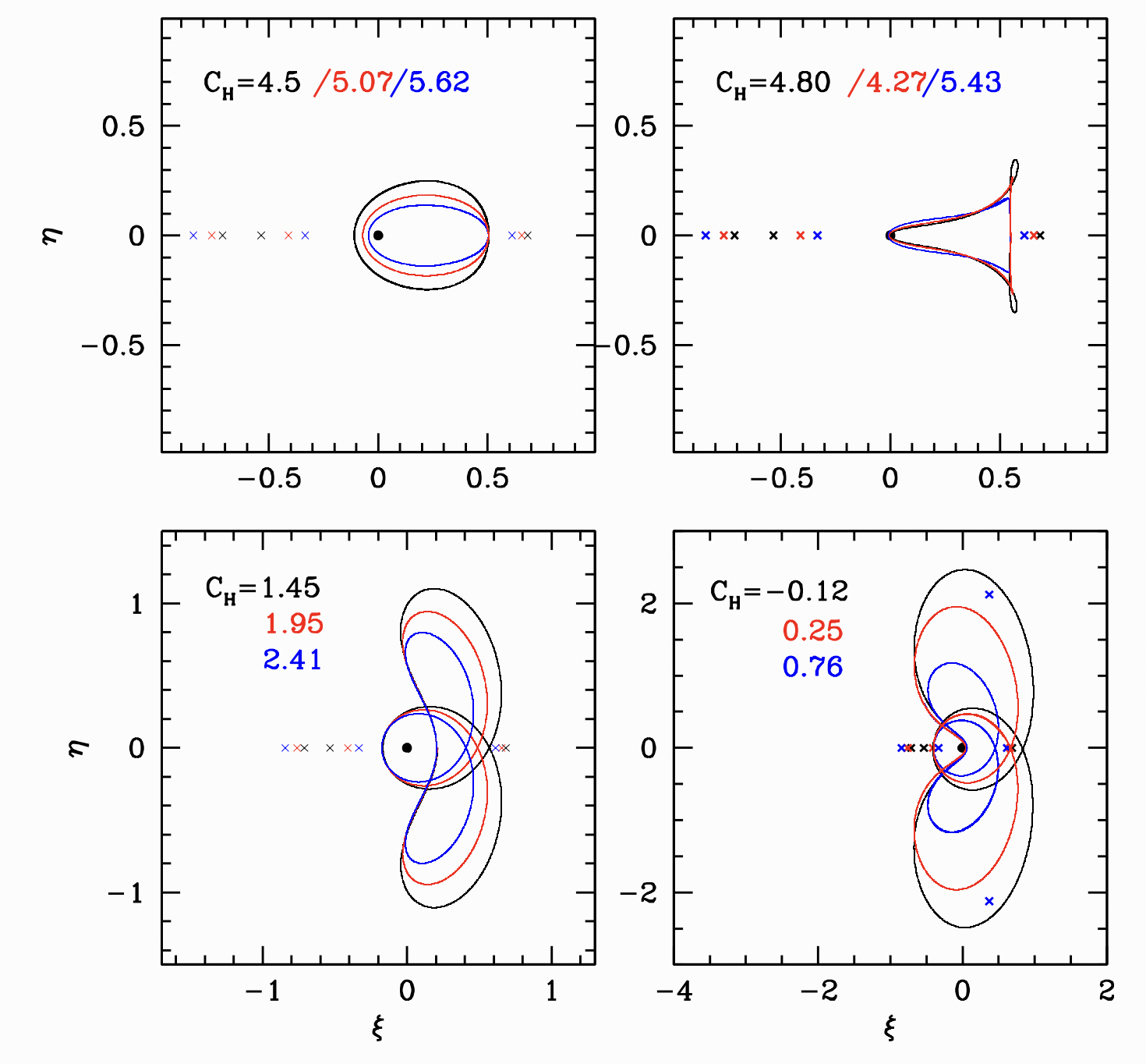
Figure 16: These panels show how the shape of the $G$ family of orbits changes with $C_{H}$. In the upper left panel, we show the equilibria with $\xi(0)=0.24$ for $\beta=0.001$(black), $\beta=0.05$ (red) and $\beta=0.1$ (blue). Also shown, as crosses, are the corresponding $L_{1}$,$L_{2}$ and $L_{2}^{\prime}$ points for each $\beta$. The upper right panel shows the equivalent for orbits close to the widest point of the stable branch in Figure 5. The lower left panel shows the shapes of the orbits after the family has become doubly periodic, and the lower right panel shows the continued evolution towards lower $C_{H}$.

Figure 17 shows the orbits of the $G^{\prime}$ family, as a function of $C_{H}$. This is composed of a combination of $g$ and $g^{\prime}$ from the $\beta=0$ case, although most of them correspond to the $g$ family. The black curves show $\beta=0.001$ and the red curves show the case for $\beta=0.05$. This family shrinks in extent as $\beta$ increases, and so there are no red curves in the upper right and lower left panels, because there are no solutions for these values of $\xi(0)$. Furthermore, there are no blue curves because this family is absent for $\beta=0.1$. We show green curves in those cases where there is no solution at $\beta=0.05$. In these cases, $C_{H}$ is chosen to have the same value for $\beta=0.001$ and $\beta=0.05$.

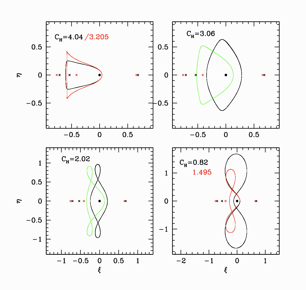
Figure 17: These panels show the evolution of the $G^{\prime}$ family of orbits. In the upper left panel, we show orbits for $\beta=0.001$ (black) and $\beta=0.05$ (red). The linear equilibrium points are shown as crosses.The two solutions have the same starting value $\xi(0)$. In the upper right and lower left, there are no solutions for $\beta=0.05$ with equivalent $\xi(0)$. In these cases, orbits with the same $C_{H}$ are shown as green curves. Finally, in the lower right, we show solutions for both $\beta$ and the same $\xi(0)$.

To complete the discussion of prograde orbital families, Figure 18 shows the evolution of family $A$ (the orbits of libration about the $L_{2}$ point), for different $C_{H}$ and $\beta=0.05$ and $\beta=0.1$. Once again, the comparison in each panel is made with fixed $\xi(0)$. We see that increasing $\beta$ makes the orbit more compact. The general shape trend is similar to that in the $\beta=0$ case, with the orbits tending towards the consecutive collision shape as $C_{H}$ becomes more negative.

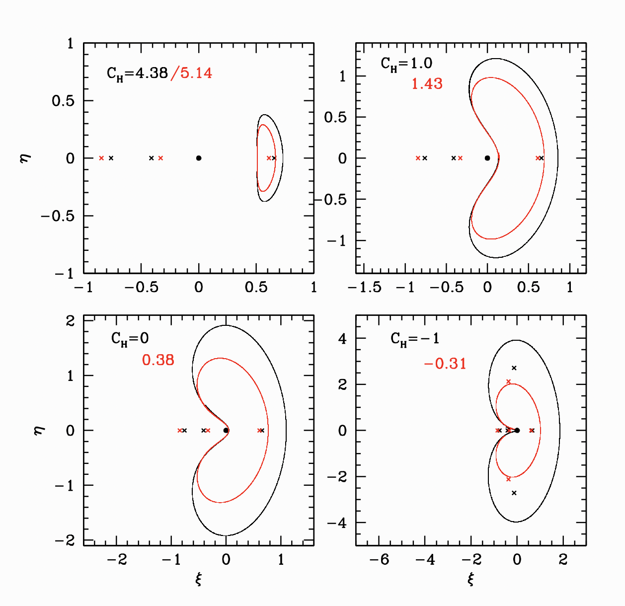
Figure 18: In each panel, the black orbits refer to the case of $\beta=0.05$ and the red orbits for $\beta=0.1$. The orbits correspond to the family $A$ of equilibria. The crosses show the locations of the respective fixed points. In particular, this family corresponds to the librations about the $L_{2}$ point. As $C_{H}$ decreases (from upper left towards lower right) the orbits acquire larger amplitudes and become more distorted.

The most important retrograde orbital family is $F$, the generalisation of Henon’s $f$ family. Figure 19 shows the evolution of this family as $C_{H}$ decreases, for $\beta=0.1$ and $\beta=0.2$. As seen previously in Figure 8, the extension of $F$ to arbitrarily large distances remains for $\beta<0.11$, but fails for larger values. This is why there is no red orbit in the bottom right panel of Figure 19.

Figure 19: These panels correspond to the famiily $F$ of retrograde orbits. In each panel, the black orbits refer to the case of $\beta=0.1$ and the red orbits for $\beta=0.2$. The crosses show the locations of the respective fixed points. The blue curves represent the $F^{\prime}$ family of the $\beta=0.1$ case. The magenta curve represents the $F^{\prime}$ solution in the case $\beta=0.2$. Once again, the overall trend with increasing $\beta$ is to make the orbits more compact.

Figure 19 also demonstrates the appearance of the second branch of the $F$ family, which we have called $F^{\prime}$. This is represented by the second asymptotic solution discussed in § 3.1, and is shown by the blue curves. The orbital shape is similar but the extension is more pronounced in the $\eta$ direction.

The $G$ curves in Figure 8 are simply the second axis crossing of those shown in Figure 17, but the $\beta>0$ cases also show a doubly periodic family $G^{\prime\prime}$ with both crossings at $\xi<0$. The shape of this family is shown in Figure 20. This family is responsible for a lot of the structure in the middle and lower panels of Figure 8. The $\beta=0.1$ case shows how the two loops converge as the solution approaches the turning point in $C_{H}$, and also how a second branch emerges to track the $F^{\prime}$ family as the doubly periodic version. The $\beta=0.2$ case does not extend over as large a range. Once again, we compare orbits with the same initial $\xi(0)$ and choose $C_{H}$ accordingly.

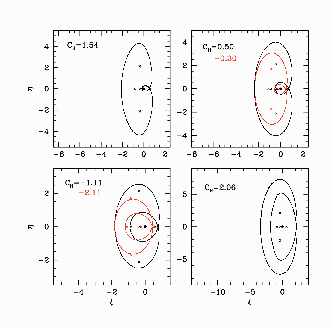
Figure 20: In each panel, the black orbits refer to the case of $\beta=0.1$ and the red orbits for $\beta=0.2$. The crosses show the locations of the respective fixed points. The blue curves represent the $F^{\prime}$ family of the $\beta=0.1$ case. Once again, the overall trend with increasing $\beta$ is to make the orbits more compact.

Figure 21 rounds out the census of orbit families, showing the Family $C$ of libration orbits about the $L_{1}$ point. As can be seen in Figure 8, for $\beta=0.1$ the family does not extend to arbitrarily large distances, and so some of the panels show only the $\beta=0.05$ case.

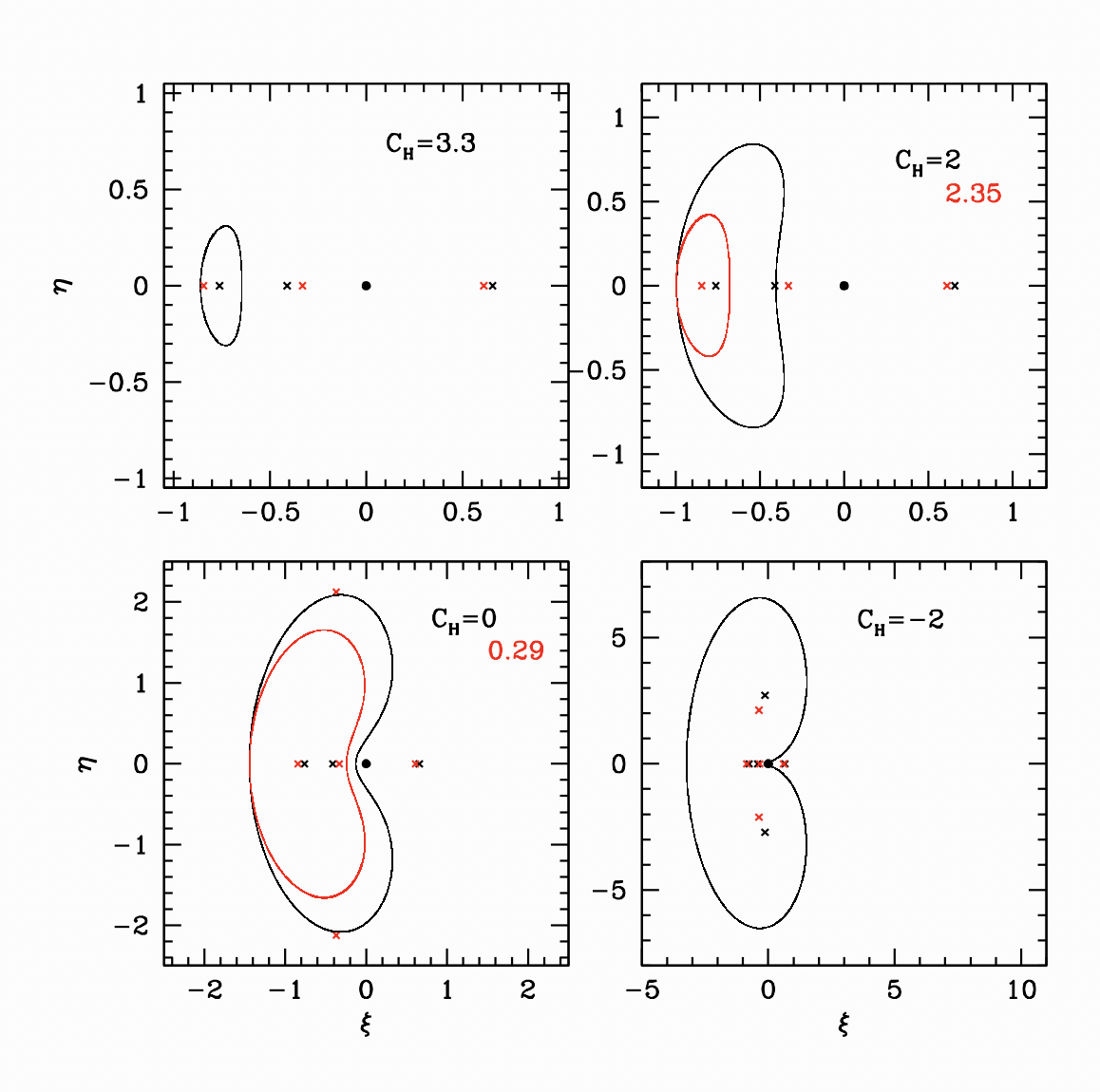
Figure 21: The equilibria shown here represent the family $C$ of librations about the $L_{1}$ point. In each panel, the black orbits refer to the case of $\beta=0.05$ and the red orbits for $\beta=0.1$. The crosses show the locations of the respective fixed points.

One of the more striking features of the $\beta=0.1$ and $\beta=0.2$ retrograde orbits is the ‘vortex-like’ structure apparent in the middle and lower panels of Figure 8. To better understand the nature of this feature, Figure 22 shows the full set of retrograde equilibria that pass through $\xi(0)=-1.9$, for the case of $\beta=0.1$. There are a total of eight different curves shown between the two panels. Some of the orbits correspond to the standard incarnations to be expected (the $F$ orbit and the leftmost $G^{\prime\prime}$ orbit) but several of the orbital families exhibit a doubling of the number of potential equilibria (this is responsible for the vortex-like structure in Figure 8).

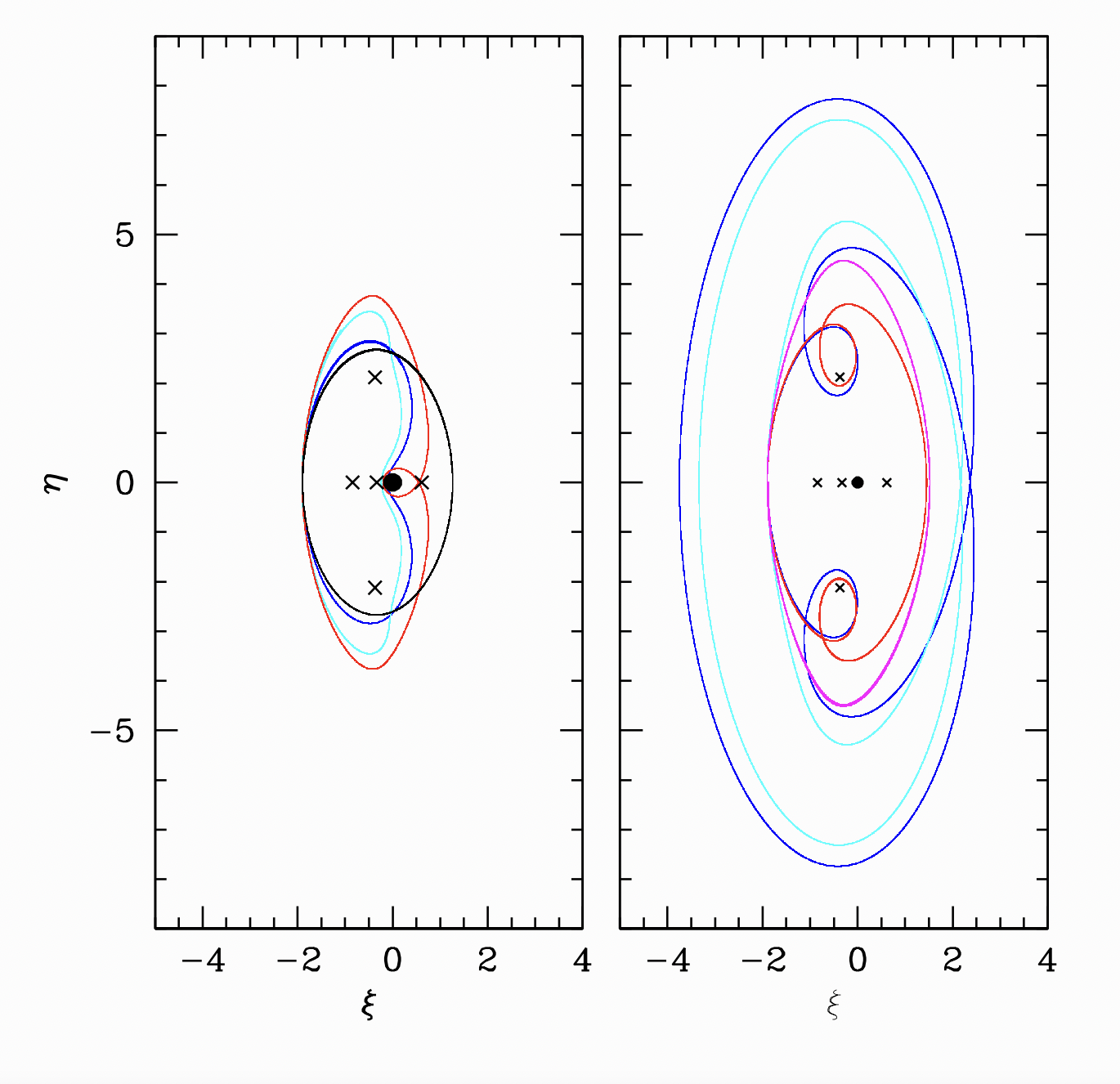
Figure 22: All orbits in this figure are equilibria for the case $\mu=0.001$, $\beta=0.1$ and with starting condition $\xi(0)=-1.9$ and $\dot{\xi}=0$. The value of $C_{H}$ is different, however. In the left hand panel, the black curve represents the $F$ family, and the red curve indicates the leftmost intersection of the $G^{\prime\prime}$ family. Finally, the blue and cyan curves represent two incarnations of the $C$ family. The right-hand panel shows two incarnations each of the $G^{\prime\prime}$ family (blue and cyan) and the $F^{\prime}$ family (red and magenta). Also show, as crosses, are the stationary points of the potential. The equivalents of the $L_{4}$ and $L_{5}$ points are responsible for the doubling of the orbital families, as can be seen by the loops induced in the red and blue curves.

We can trace the extra orbits to the appearance of the $L_{4}$/$L_{5}$ analogues (shown as crosses in Figure 22) because we note that several of the new orbits retain the overall shape of the parent family, but feature an extra loop around the equilibrium point (compare the blue and cyan orbits in the right hand panel, or the red and magenta orbits). So, we can trace the extra features in the orbital distribution to the presence of these potential minima, which affect the orbital shape if the orbit passes too close to them.

Appendix B B: Heliocentric Parameters

In order to determine whether a directly imaged feature is bound to the host star, one measures the proper motion (and radial velocity, if one is lucky) relative to the star and converts the results into a set of Keplerian orbital parameters. If the object is experiencing additional accelerations due to an unseen companion, the resulting parameters may take values different from those expected given the position relative to the star.

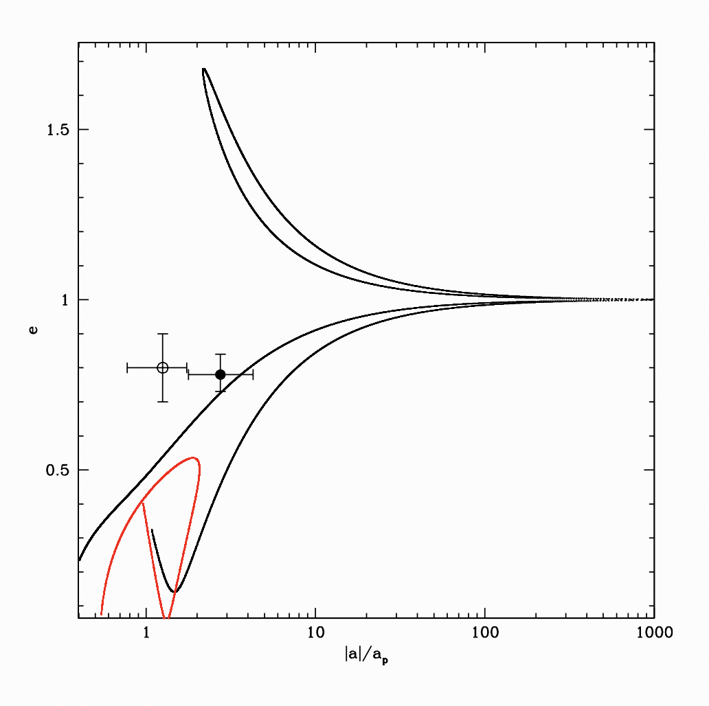
Figure 23: The red curve shows the inferred heliocentric parameters for a quasi-satellite orbit drawn from the $F$ family, in the case $\mu=0.001$ and $\beta=0.1$. The initial conditions were $C_{H}=-5$ and $\xi(0)=-4.1455$. The black curve shows the equivalent for a member of the $F^{\prime}$ orbital family, with $C_{H}=5.85$ and $\xi(0)=-5$. The solid point represents the Fom b parameters estimated by Gaspar & Riecke (2020) and the open point those from Kalas et al. (2013). Semi-major axis is measured relative to the planet (which is taken to be the dust ring median for the observations). We note again the black curve is a bound equilibrium simply periodic orbit – the unbound heliocentric parameters are the result of accelerations due to the planet and not modelled in the Keplerian fit.

Figure 23 shows the calculated heliocentric Keplerian semi-major axis and eccentricity for two example quasi-satellite orbits – one from the $F$ family (shown in red) and one from the $F^{\prime}$ (shown in black). These are both examples of stable quasi-satellite orbits for the case of $\mu=0.001$ and $\beta=0.1$. We see that, during the wide excursions relative to the planet, the inferred heliocentric parameters can vary wildly, including reaching apparently unbound values in the case of the $F^{\prime}$ orbit. We also compare this to the values inferred for the dusty object Fomalhaut b Kalas et al. (2013); Gaspar & Rieke (2020). The inferred orbital parameters of this object were the result of much discussion in the past, but are quite consistent with dust in a quasi-satellite orbit. We discuss this more directly in § 5.2.1.

References

- Boley et al. (2012) Boley A. C., Payne M. J., Corder S., Dent W. R. F., Ford E. B., Shabram M., 2012, \hrefhttp://dx.doi.org/10.1088/2041-8205/750/1/L21 ApJ, \hrefhttps://ui.adsabs.harvard.edu/abs/2012ApJ…750L..21B 750, L21
- Burns et al. (1979) Burns J. A., Lamy P. L., Soter S., 1979, \hrefhttp://dx.doi.org/10.1016/0019-1035(79)90050-2 Icarus, \hrefhttps://ui.adsabs.harvard.edu/abs/1979Icar…40….1B 40, 1
- Chiang et al. (2009) Chiang E., Kite E., Kalas P., Graham J. R., Clampin M., 2009, \hrefhttp://dx.doi.org/10.1088/0004-637X/693/1/734 ApJ, \hrefhttps://ui.adsabs.harvard.edu/abs/2009ApJ…693..734C 693, 734
- Currie et al. (2012) Currie T., et al., 2012, \hrefhttp://dx.doi.org/10.1088/2041-8205/760/2/L32 ApJ, \hrefhttps://ui.adsabs.harvard.edu/abs/2012ApJ…760L..32C 760, L32
- Dohnanyi (1969) Dohnanyi J. S., 1969, \hrefhttp://dx.doi.org/10.1029/JB074i010p02531 J. Geophys. Res., \hrefhttps://ui.adsabs.harvard.edu/abs/1969JGR….74.2531D 74, 2531
- Domingos et al. (2006) Domingos R. C., Winter O. C., Yokoyama T., 2006, \hrefhttp://dx.doi.org/10.1111/j.1365-2966.2006.11104.x MNRAS, \hrefhttps://ui.adsabs.harvard.edu/abs/2006MNRAS.373.1227D 373, 1227
- Galicher et al. (2013) Galicher R., Marois C., Zuckerman B., Macintosh B., 2013, \hrefhttp://dx.doi.org/10.1088/0004-637X/769/1/42 ApJ, \hrefhttps://ui.adsabs.harvard.edu/abs/2013ApJ…769…42G 769, 42
- García Yárnoz et al. (2015) García Yárnoz D., Scheeres D. J., McInnes C. R., 2015, \hrefhttp://dx.doi.org/10.1007/s10569-015-9604-9 Celestial Mechanics and Dynamical Astronomy, \hrefhttps://ui.adsabs.harvard.edu/abs/2015CeMDA.121..365G 121, 365
- Gaspar & Rieke (2020) Gaspar A., Rieke G., 2020, \hrefhttp://dx.doi.org/10.1073/pnas.1912506117 Proceedings of the National Academy of Science, \hrefhttps://ui.adsabs.harvard.edu/abs/2020PNAS..117.9712G 117, 9712
- Gáspár et al. (2023) Gáspár A., et al., 2023, \hrefhttp://dx.doi.org/10.1038/s41550-023-01962-6 Nature Astronomy, \hrefhttps://ui.adsabs.harvard.edu/abs/2023NatAs.tmp…93G
- Giancotti et al. (2014) Giancotti M., Campagnola S., Tsuda Y., Kawaguchi J., 2014, \hrefhttp://dx.doi.org/10.1007/s10569-014-9564-5 Celestial Mechanics and Dynamical Astronomy, \hrefhttps://ui.adsabs.harvard.edu/abs/2014CeMDA.120..269G 120, 269
- Giuppone et al. (2010) Giuppone C. A., Beaugé C., Michtchenko T. A., Ferraz-Mello S., 2010, \hrefhttp://dx.doi.org/10.1111/j.1365-2966.2010.16904.x MNRAS, \hrefhttps://ui.adsabs.harvard.edu/abs/2010MNRAS.407..390G 407, 390
- Hamilton & Burns (1991) Hamilton D. P., Burns J. A., 1991, \hrefhttp://dx.doi.org/10.1016/0019-1035(91)90039-V Icarus, \hrefhttps://ui.adsabs.harvard.edu/abs/1991Icar…92..118H 92, 118
- Hamilton & Krivov (1996) Hamilton D. P., Krivov A. V., 1996, \hrefhttp://dx.doi.org/10.1006/icar.1996.0175 Icarus, \hrefhttps://ui.adsabs.harvard.edu/abs/1996Icar..123..503H 123, 503
- Hayakawa & Hansen (2023) Hayakawa K. T., Hansen B. M. S., 2023, \hrefhttp://dx.doi.org/10.1093/mnras/stad1091 MNRAS, \hrefhttps://ui.adsabs.harvard.edu/abs/2023MNRAS.522.2115H 522, 2115
- Henon (1969) Henon M., 1969, A&A, \hrefhttps://ui.adsabs.harvard.edu/abs/1969A&A…..1..223H 1, 223
- Henon (1970) Henon M., 1970, A&A, \hrefhttps://ui.adsabs.harvard.edu/abs/1970A&A…..9…24H 9, 24
- Hill (1878a) Hill G. W., 1878a, Am. J. Math., \hrefnone 1, 5
- Hill (1878b) Hill G. W., 1878b, Am. J. Math., \hrefnone 1, 129
- Hill (1878c) Hill G. W., 1878c, Am. J. Math., \hrefnone 1, 245
- Hunter (1967) Hunter R. B., 1967, \hrefhttp://dx.doi.org/10.1093/mnras/136.3.245 MNRAS, \hrefhttps://ui.adsabs.harvard.edu/abs/1967MNRAS.136..245H 136, 245
- Jewitt (2012) Jewitt D., 2012, \hrefhttp://dx.doi.org/10.1088/0004-6256/143/3/66 AJ, \hrefhttps://ui.adsabs.harvard.edu/abs/2012AJ….143…66J 143, 66
- Jewitt & Haghighipour (2007) Jewitt D., Haghighipour N., 2007, \hrefhttp://dx.doi.org/10.1146/annurev.astro.44.051905.092459 ARA&A, \hrefhttps://ui.adsabs.harvard.edu/abs/2007ARA&A..45..261J 45, 261
- Kalas et al. (2005) Kalas P., Graham J. R., Clampin M., 2005, \hrefhttp://dx.doi.org/10.1038/nature03601 Nature, \hrefhttps://ui.adsabs.harvard.edu/abs/2005Natur.435.1067K 435, 1067
- Kalas et al. (2008) Kalas P., et al., 2008, \hrefhttp://dx.doi.org/10.1126/science.1166609 Science, \hrefhttps://ui.adsabs.harvard.edu/abs/2008Sci…322.1345K 322, 1345
- Kalas et al. (2013) Kalas P., Graham J. R., Fitzgerald M. P., Clampin M., 2013, \hrefhttp://dx.doi.org/10.1088/0004-637X/775/1/56 ApJ, \hrefhttps://ui.adsabs.harvard.edu/abs/2013ApJ…775…56K 775, 56
- Kanavos et al. (2002) Kanavos S. S., Markellos V. V., Perdios E. A., Douskos C. N., 2002, \hrefhttp://dx.doi.org/10.1023/A:1026238123759 Earth Moon and Planets, \hrefhttps://ui.adsabs.harvard.edu/abs/2002EM&P…91..223K 91, 223
- Kennedy & Wyatt (2011) Kennedy G. M., Wyatt M. C., 2011, \hrefhttp://dx.doi.org/10.1111/j.1365-2966.2010.18041.x MNRAS, \hrefhttps://ui.adsabs.harvard.edu/abs/2011MNRAS.412.2137K 412, 2137
- Kennedy et al. (2023) Kennedy G. M., Lovell J. B., Kalas P., Fitzgerald M. P., 2023, \hrefhttp://dx.doi.org/10.48550/arXiv.2305.10480 arXiv e-prints, \hrefhttps://ui.adsabs.harvard.edu/abs/2023arXiv230510480K p. arXiv:2305.10480
- Kushvah (2008) Kushvah B. S., 2008, \hrefhttp://dx.doi.org/10.1007/s10509-008-9823-6 Ap&SS, \hrefhttps://ui.adsabs.harvard.edu/abs/2008Ap&SS.315..231K 315, 231
- Markellos et al. (2000) Markellos V. V., Roy A. E., Velgakis M. J., Kanavos S. S., 2000, \hrefhttp://dx.doi.org/10.1023/A:1002487228086 Ap&SS, \hrefhttps://ui.adsabs.harvard.edu/abs/2000Ap&SS.271..293M 271, 293
- Mikkola & Innanen (1997) Mikkola S., Innanen K., 1997, in Dvorak R., Henrard J., eds, The Dynamical Behaviour of our Planetary System. p. 345
- Murray & Dermott (2000) Murray C. D., Dermott S. F., 2000, Solar System Dynamics, \hrefhttp://dx.doi.org/10.1017/CBO9781139174817. doi:10.1017/CBO9781139174817.
- Nesvorný et al. (2003) Nesvorný D., Alvarellos J. L. A., Dones L., Levison H. F., 2003, \hrefhttp://dx.doi.org/10.1086/375461 AJ, \hrefhttps://ui.adsabs.harvard.edu/abs/2003AJ….126..398N 126, 398
- Perdiou et al. (2012) Perdiou A. E., Perdios E. A., Kalantonis V. S., 2012, \hrefhttp://dx.doi.org/10.1007/s10509-012-1145-z Ap&SS, \hrefhttps://ui.adsabs.harvard.edu/abs/2012Ap&SS.342…19P 342, 19
- Quillen (2006) Quillen A. C., 2006, \hrefhttp://dx.doi.org/10.1111/j.1745-3933.2006.00216.x MNRAS, \hrefhttps://ui.adsabs.harvard.edu/abs/2006MNRAS.372L..14Q 372, L14
- Radzievskii (1950) Radzievskii V. V., 1950, AZh, \hrefhttps://ui.adsabs.harvard.edu/abs/inothtere 27, 250
- Radzievskii (1953) Radzievskii V. V., 1953, AZh, \hrefhttps://ui.adsabs.harvard.edu/abs/inothtere 30, 265
- Schuerman (1980) Schuerman D. W., 1980, \hrefhttp://dx.doi.org/10.1086/157989 ApJ, \hrefhttps://ui.adsabs.harvard.edu/abs/1980ApJ…238..337S 238, 337
- Simmons et al. (1985) Simmons J. F. L., McDonald A. J. C., Brown J. C., 1985, \hrefhttp://dx.doi.org/10.1007/BF01227667 Celestial Mechanics, \hrefhttps://ui.adsabs.harvard.edu/abs/1985CeMec..35..145S 35, 145
- Tremaine (2023) Tremaine S., 2023, Dynamics of Planetary Systems
- Wiegert et al. (2000) Wiegert P., Innanen K., Mikkola S., 2000, \hrefhttp://dx.doi.org/10.1086/301291 AJ, \hrefhttps://ui.adsabs.harvard.edu/abs/2000AJ….119.1978W 119, 1978
- Zotos (2015) Zotos E. E., 2015, \hrefhttp://dx.doi.org/10.1007/s10509-015-2513-2 Ap&SS, \hrefhttps://ui.adsabs.harvard.edu/abs/2015Ap&SS.360….1Z 360, 1