Stable Coronal X-Ray Emission Over Twenty Years of XZ Tau

Abstract

XZ Tau AB is a frequently observed binary YSO in the Taurus Molecular Cloud; XZ Tau B has been classified as an EXOr object. We present new Chandra/HETG-ACIS-S observations of XZ Tau AB, complemented with variability monitoring of the system with XMM-Newton, to constrain the variability of this system and identify high-resolution line diagnostics to better understand the underlying mechanisms that produce the X-rays. We observe two flares with XMM-Newton, but find that outside of these flares the coronal X-ray spectrum of XZ Tau AB is consistent over twenty years of observations. We compare the ensemble of XZ Tau X-ray observations over time with the scatter across stars observed in point-in-time observations of the Orion Nebula Cluster and find that both overlap in terms of plasma properties, i.e., some of the scatter observed in the X-ray properties of stellar ensembles stems from intrinsic source variability.

1 Introduction

Stars and their circumstellar disks form as a result of gravitational contraction of molecular clouds. The early stages of low-mass ($<2M_{\odot}$) stellar evolution are characterized by violent accretion events, large molecular outflows and jets as star-disk systems clear their surrounding environment. A subset of pre-MS stars undergoing this violent accretion are part of an observationally rare but important class called FUor and EXor (after their namesakes FU Ori and EX Lup). These objects undergo extreme mass accretion events ($\Delta\mathbf{\dot{M}}\sim 10^{2-4}$) where their optical brightness can increase by $\Delta V\sim 3-5$ (Audard et al., 2014). FUor and EXor objects are distinguished by their outburst intensity and frequency: FUors exhibit brighter $\Delta V\sim 3-5$ mag events which last years-centuries, while EXors undergo less intense but more frequent outbursts on timescales of months-years. While it is clear FUor/EXors drastically increase in magnitude as a result of sudden accretion, it is debated as to why these objects undergo these intense mass accretion events. Several theories have been proposed including: disk fragmentation (Vorobyov, 2013) and/or perturbations from a binary component or massive planet causing disk instabilities (Clarke et al., 1990) or even the “consumption” of tidally disrupted protoplanets.

X-ray emission is ubiquitous among low-mass pre-MS stars due to their convective zones and fast rotational periods which generate strong magnetic dynamos. In particular, several distinct physical mechanisms are capable of producing X-rays in pre-MS stars: magnetically heated coronae with characteristic temperatures of $\sim 0.1-10.0$ keV that result in continuum and line emission dependent on coronal abundances (e.g. Preibisch et al., 2005; Scelsi et al., 2007), shock-heated plasma (at characteristic temperatures of $\sim 0.3$ keV) as a result of mass funneled from the circumstellar disk along magnetic field lines and onto the star (see review by Schneider et al., 2022), and star-disk magnetic reconnection events which can magnetically heat material to temperatures in excess of $\sim 8.6$ keV (Favata et al., 2005). A multiwavelength campaign to study the outburst of FUor/EXor type object V1647 Ori detected a $\sim 2$ order of magnitude increase in X-ray flux associated with star-disk magnetospheric interactions (Kastner et al., 2004). A handful of cases have also been identified where angular momentum is lost as jets launched from the system during the Class II stage, which are also seen in X-rays (Pravdo et al., 2001; Favata et al., 2002; Schneider et al., 2011), mostly from plasma with $kT\approx 0.3$ keV (e.g. Grosso et al., 2006; Bonito et al., 2007). This X-ray emission likely comes from shock-heated material traveling away from the source with velocities in excess of 300 km s^-1 (see, e.g., DG Tau, Güdel et al., 2008; Schneider & Schmitt, 2008). X-ray observations of FUor/EXor type objects have revealed indications of X-ray emitting jets (Stelzer et al., 2009, Z Cma), X-ray bright accretion hot spots (Hamaguchi et al., 2012), and magnetic reconnection events (Kastner et al., 2004).

Eventually, pre-MS stars clear out their surrounding molecular envelopes and disks and thus lose many of the above physical mechanisms capable of producing X-rays even while they remain coronally active. Therefore, it is imperative to investigate features during this young, embedded stage of stellar evolution to understand how stars evolve and, in particular, investigate what impact these sources of X-rays have on circumstellar disks and the eventual formation of planets (Owen et al., 2011; Skinner & Güdel, 2013; Cleeves et al., 2013). While numerous studies have been published revealing a wealth of data regarding star formation (Getman et al., 2005; Güdel et al., 2007), the vast majority of the observational work has been limited to single snapshots in time for a variety of objects, rather than tracking particular sources over longer time periods. One potential source to analyze over this longer time frame is the YSO binary system XZ Tau.

1.1 The XZ Tau AB system

XZ Tau AB is a close separation binary with $a\sim 0.3^{\prime\prime}$ or 42 au (Haas et al., 1990) composed of an M1 and an M2 pre-MS star. Each member hosts its own circumstellar disk (Zapata et al., 2015), and their small separation likely induces disk disruptions leading to mass accretion events. Optical spectroscopy resolving the binary has demonstrated that each member is a highly accreting source (White & Ghez, 2001). Moreover, the spectrum of XZ Tau B is heavily veiled and shows spectral features similar to that of DG Tau, a star-disk system with intense accretion and an observed jet resolved at both optical and X-ray wavelengths (Güdel et al., 2008). Both XZ Tau A and XZ Tau B exhibit jets at optical wavelengths (Krist et al., 2008) while a complex bubble-like system encompasses both stars.

ALMA 1.3mm continuum observations have detected dust emission associated with both circumstellar disks. 12CO emission traces collimated outflows surrounding the XZ Tau A system, typically a signature of youth (Zapata et al., 2015; Arce & Sargent, 2006). The 1.3mm continuum detection of XZ Tau B indicates an unusually small circumstellar disk with a radius of only 3.6 AU and an inner cavity of 1.3 AU that the authors attribute to ongoing planet formation (Osorio et al., 2016). Such a small disk may be unable to sufficiently shield itself from intense X-ray irradiation and thus the impact on planet formation should be investigated. The classification of XZ Tau B as an EXor object (Coffey et al., 2004; Lorenzetti et al., 2009) in combination with its unusually high accretion rate and small disk suggests this pre-MS star may be going through rapid stellar evolution and its disk may not survive for much longer.

XZ Tau AB has been observed with multiple X-ray instruments between 1990 and the present and displays both long and short term variability. None of these observations are able to resolve the $\sim 0.3^{\prime\prime}$ binary; Chandra’s PSF comes close but does not achieve it, while XMM-Newton is incapable of it, as seen in Figure 1. Favata et al. (2003) reported variability during their $\sim 50$ ks observation of XZ Tau AB. While the count rate increased linearly during the observation, $N_{H}$ decreased from $1.06\times 10^{22}\mathrm{cm}^{-2}$ to $0.26\times 10^{22}\mathrm{cm}^{-2}$ while the plasma temperature increased by a similar factor. An emission measure ratio of $\sim{1300}$ between the soft (0.14 keV) and hard (2.29 keV) temperature component at the onset of the count rate increase strongly suggest the presence of either accretion or jet emission. In 2006, a five day monitoring campaign of XZ Tau AB displayed only low levels of $N_{H}\sim 0.1\times 10^{22}\mathrm{cm}^{-2}$ with $\mathrm{kT_{X1}},\mathrm{kT_{X2}}=0.84$ keV and 4.6 keV respectively, although spectral analysis was complicated by extensive background emission during the observation. Giardino et al. (2006) presented a re-analysis of the Favata et al. (2003) data, showing that the variable X-ray spectrum could be fit with either a low or high $N_{H}$ depending on the coronal abundances assumed in the model. However, none of these observations incorporate high-resolution gratings spectra, potentially capable of breaking degeneracies between X-ray emission mechanisms by enabling resolution of temperature- and density-sensitive line ratios (e.g. Mg XI, Ne IX, OVII; Huenemoerder et al., 2007; Kastner et al., 2002; Brickhouse et al., 2010).

In this paper, we present new observations of XZ Tau AB with Chandra/HETG, complemented with observations with XMM-Newton collected as part of a larger X-ray monitoring campaign on the Taurus star-forming region to constrain variability observed in the Chandra observations. Using these data, we analyze the present-day state of XZ Tau AB, in comparison to previous observations. We also present contemporaneous ground-based optical observations to assess whether XZ Tau AB was in outburst during the most recent Chandra and XMM-Newton observations.

We discuss the observations and data reduction methods in Sect. 2. In Section 3 we summarize the characteristics of our observed X-ray data. In Section 4 we outline the implications of these observations, and compare our assessments to past work. We summarize our work in Section 5.

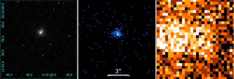
Figure 1: XZ Tau and its environs; all three panels are on the same spatial scale. Left: 2004 HST/ACS/F625W image of XZ Tau AB. Middle: 2018 Chandra/ACIS observations (obsid 21948 shown here) do not resolve XZ Tau AB, but have a tight PSF with low background. Right: 2020 XMM-Newton observations (obsid 0865040201 shown here) have more counts, but a much wider PSF.

2 Observations and Data Reduction

We summarize our new observations in Table 1. Below, we briefly describe the observations and data reduction.

Table 1: Summary of New Observations of XZ Tau AB

obsid	Telescope/Instrument	Start (MJD)	Start Date (UTC)	Duration (ks)
21946	Chandra/ACIS/HETG	58415.68640	2018-10-24	12.0
20160	Chandra/ACIS/HETG	58417.26343	2018-10-26	41.5
21947	Chandra/ACIS/HETG	58418.28612	2018-10-27	12.0
21948	Chandra/ACIS/HETG	58418.62041	2018-10-27	56.0
20161	Chandra/ACIS/HETG	58419.90608	2018-10-28	48.5
21950	Chandra/ACIS/HETG	58421.71834	2018-10-30	14.0
21951	Chandra/ACIS/HETG	58422.54435	2018-10-31	36.5
21952	Chandra/ACIS/HETG	58424.40864	2018-11-02	12.5
21953	Chandra/ACIS/HETG	58425.19608	2018-11-03	36.5
21954	Chandra/ACIS/HETG	58433.72045	2018-11-11	25.5
21965	Chandra/ACIS/HETG	58434.31770	2018-11-12	25.5
0865040201	XMM-Newton/EPIC	59079.67552	2020-08-18	36.8
0865040301	XMM-Newton/EPIC	59083.65674	2020-08-22	40.0
0865040401	XMM-Newton/EPIC	59089.81463	2020-08-28	33.0
0865040601	XMM-Newton/EPIC	59095.94792	2020-09-03	33.0
0865040701	XMM-Newton/EPIC	59104.26799	2020-09-12	33.0
0865040501	XMM-Newton/EPIC	59110.54296	2020-09-18	47.9

2.1 Chandra

XZ Tau AB was observed by Chandra eleven times over the span of three weeks, from 2018 October 24 through 2018 November 12, with the High-Energy Transmission Grating Spectrograph (HETGS) (Canizares et al., 2005). The aimpoint was centered between XZ Tau AB and HL Tau, with the goal of observing both sources in parallel. Data were reduced with the Chandra Interactive Analysis software (CIAO; v. 4.14). The observations were energy filtered (0.5-8.0 keV) and time-filtered on good time intervals to reduce flaring particle background. Zeroth-order and gratings spectra were extracted with standard procedures in CIAO.

2.2 XMM-Newton

XZ Tau AB was observed by the X-ray Multimirror Mission (XMM-Newton) observatory six times over the course of 33 days from 2020 August 18 through 2020 September 19, as part of a larger campaign to monitor variability of young stellar objects in Taurus (PI Schneider). The observations used the medium thickness optical blocking filter. XZ Tau and HL Tau were extracted using standard procedures in SAS version 19.1.0. Because of the close proximity of XZ Tau AB and HL Tau, we defined custom extraction regions to ensure minimal contamination of each source by the other source. The observations were energy filtered (0.3-8.0 keV) and time-filtered on good time intervals to reduce flaring particle background.

2.3 AAVSO

The two components of XZ Tau AB are known to be variable in the optical over the course of years, indicating potential outbursts expected of an ExOr object (Krist et al., 2008). To track the state of the XZ Tau AB and HL Tau systems, we requested observations of XZ Tau AB and HL Tau from the Association of Amateur Variable Star Observers (AAVSO) over the time periods of observation by Chandra and XMM. These observations, distributed across multiple observers, provide low-cadence optical monitoring over the course of the observations. While the AAVSO data do not resolve the separate components of XZ Tau A and B, Krist et al. (2008) resolves the two components with HST and find that XZ Tau A is relatively stable ($R$ magnitude changes $\sim 0.6$ mag between 1995 and 2004), while XZ Tau B can exhibit wide variations ($R$ magnitude changes $\sim 3.23$ mag between 2001 and 2004), which suggests that the bulk of the intrinsic variability is due to XZ Tau B.

3 Analysis

3.1 Identifying Components

We attempted to determine if the two components of XZ Tau AB were resolvable in the Chandra data, using the positions for the stars recorded by ALMA (Ichikawa et al., 2021). While XZ Tau A and B are separated by $\sim 0.3^{\prime\prime}$ (Ichikawa et al., 2021), the Chandra and XMM point spread functions (PSFs) are too wide to precisely pinpoint whether the X-rays are coming from one star, or both–the center of the X-ray source in the Chandra data is offset from both of the two ALMA sources ($0^{\prime\prime}.35$ north of XZ Tau A, $0^{\prime\prime}.26$ east of XZ Tau B). We thus treat all of our observations as the combined spectrum of both components.

3.2 Was XZ Tau AB in Outburst During the New X-Ray Observations?

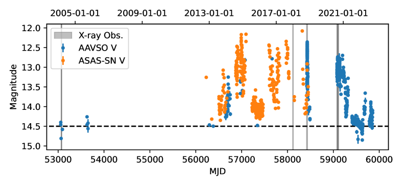
Figure 2: $V$-band light curve for XZ Tau AB from the AAVSO and ASAS-SN. The black dashed line represents the estimated baseline level for when XZ Tau B is not in an elevated state. Gray windows highlight times of X-ray observations in 2004, 2017, 2018, and 2020. “Zoomed-in” light curves for individual X-ray observations are shown in Figures 3 and 4.

We considered the full light curve for XZ Tau provided by the AAVSO, and used it to generate color light curves for each observation. Analyzing color as a function of time as well as the observed brightness should mitigate uncertainty in recorded brightness due to differences in observing setup for each observer. It also allows for evaluation of the extinction of the star as a function of time, which yields insight into the behavior of the circumstellar dust. To supplement the AAVSO light curves and serve as a “ground truth” measure of XZ Tau AB’s brightness, we also considered the V-band light curve of XZ Tau from the ASAS-SN catalog of variable stars (Shappee et al., 2014; Jayasinghe et al., 2019).

Based on Hubble Space Telescope images of the resolved components of the XZ Tau system, Giardino et al. (2006) found that while XZ Tau B was potentially in outburst when the XZ Tau system was first observed with XMM-Newton in 2000, it had clearly subsided by the time of the 2004 XMM-Newton observations. Krist et al. (2008) found similar results.

The full AAVSO+ASAS-SN $V$-magnitude light curve for XZ Tau AB is presented in Figure 2, with the timeframes of various X-ray observations (including the 2018 Chandra and 2020 XMM-Newton observations) highlighted. We estimate the baseline “quiescent” level of the total $V$-band light from XZ Tau AB outside of outburst from the AAVSO data contemporaneous with the XMM-Newton observations presented in Giardino et al. (2006), as these observations were taken outside of outburst based on HST imaging that resolved both components of the system.

Over the twenty-year timeframe we consider, we see periods of quiescence of duration $\sim$ one year, in 2022. We also observe clear brightening events of durations that would suggest multiple EXOr-like outbursts, including ongoing outbursts during the 2018 Chandra and 2020 XMM-Newton observations. The 2017 Chandra observations (Skinner & Güdel, 2020) appear to take place during a local minimum of optical brightness, but at an elevated optical brightness compared to the baseline set in 2004.

3.3 X-ray Time Series

The zeroth-order (non-dispersed) count rate for XZ Tau AB in the individual Chandra observations is too low to produce a light curve with detailed time resolution. We instead look at the count rates for each observation as a whole.

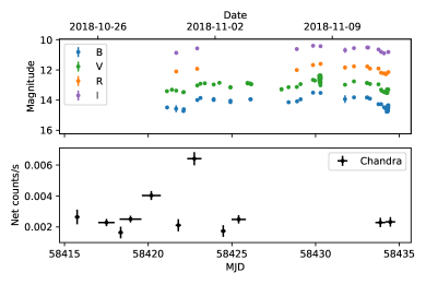
Figure 3: bottom: Zeroth-order observation-averaged net count rates for each Chandra observation of XZ Tau AB in Table 1. Error bars in the time dimension indicate the duration of each observation. Two observations (obsids 20161 and 21951) show enhanced count rates compared to the other nine observations. top: Contemporaneous AAVSO data shows some rolling variability with no obvious correlation to the Chandra variability.

We find that two of the eleven observations have significantly elevated count rates compared to the remaining nine, as depicted in Figure 3. For initial consideration, we treated these two bright observations separately, and combined the data from the remaining nine observations for improved statistics.

We present light curves from XMM-Newton with a 1000-s cadence in Figure 4. The XMM-Newton data have more counts than the Chandra observations, enabling assessment of source variability on timescales shorter than the observation itself. Four of the XMM-Newton observations are fairly stable in both low- and high-energy bands (defined as below and above 1 keV respectively). However, two observations are much brighter. The light curves of the six XMM-Newton observations clearly indicate that the observations on 2020 August 28-29 and 2020 September 3-4 are flaring, with peak brightnesses $\sim 12\times$ the median for all observations in the hard band, and $\sim 5.5\times$ the median for all observations in the soft band, even after correcting for the high background at points during these observations.

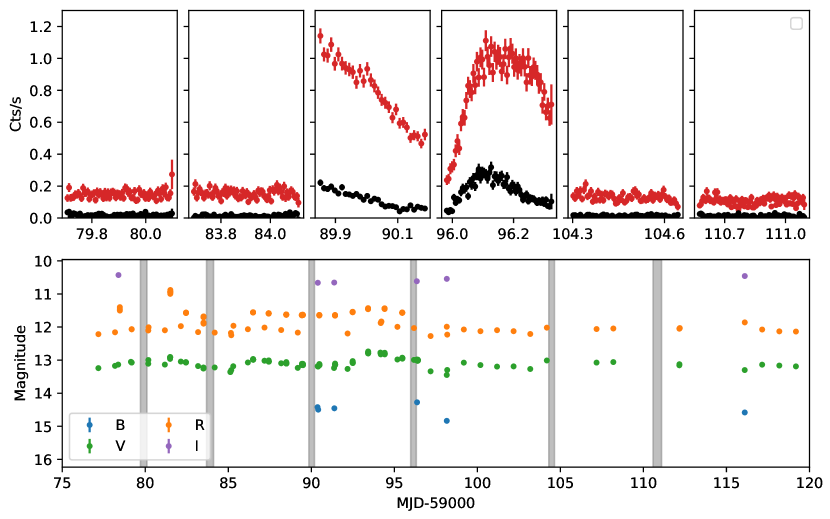
Figure 4: Broad-band light curves of XZ Tau AB from XMM-Newton (top) and AAVSO (bottom). The upper plots depict the individual XMM observations in chronological order, presenting the hard- ($>1$ keV, black) and soft-energy ($<1$ keV, red) count rates from the EPIC-PN. The bottom light curve depicts observations of XZ Tau AB from AAVSO, with the XMM-Newton observing windows highlighted in gray. Error bars are smaller than plot symbols. There is no apparent correlation in the X-ray and optical variability.

3.4 Modeling spectra

We assume that the X-ray data are adequately described by two optically thin, collisionally excited emission components (APEC models Foster et al., 2012) in collisional equilibrium, assumed to be “cool” and “hot,” multiplied by a photoelectric absorption phabs component to model interstellar and circumstellar absorption.

We also set neon and iron abundances as free parameters, and pin the abundances of nickel, silicon, calcium, and magnesium (which have similar first ionization potentials to iron) to the iron abundance. As a baseline, we fit the four “quiescent” observations from XMM-Newton jointly, and use the temperatures, normalizations, absorption column density, and abundances from that fit as the initial guess for fitting each individual observation. We list the best-fit parameters for these models with free abundances in Table 5.

Because of the diminished effective area of ACIS at low energies caused by contamination, we fixed $N_{H}$ for the Chandra observations at the best-fit $N_{H}$ for the quiescent XMM-Newton observations to mitigate degeneracy between soft plasma and hydrogen absorption. We fit the zeroth-order spectrum for each “bright” Chandra observation, but did not attempt to find individual fits for each of the faint Chandra observations. Rather, we fit the combined zeroth-order spectrum for the other nine observations. We find that the model fits to the bright observations show no significant difference from the fit to the combined faint observations due to the substantial uncertainties that result from the limited number of counts. We therefore fit the combined zeroth-order spectrum from all eleven observations. In addition to fitting all spectra with free Ne and Fe abundances, we fixed Ne and Fe abundances at the best-fit values from the joint fit to the four quiescent XMM-Newton observations and then fit all observations again; we list the best-fit parameters for these models with fixed abundances in Table 2.

We plot the PN spectra for one typical quiescent observation (obsid 0865040501) and the two flaring observations in Figure 5, with best fit models. As expected, the two flare spectra are brighter than the quiescent spectrum. Notably, the high-energy slopes of the flaring spectra are different from the quiescent spectrum, indicating a different high-energy state for those spectra. We explore time-resolved spectroscopy of the flares in Section 3.5. This recalls a similar difference in spectral shape from 2000 to 2004 identified in Giardino et al. (2006)—a hard plasma component readily apparent in the XMM-Newton spectrum from 2000 was no longer seen in 2004. Also notable in the flare observations is the presence of 6.7 keV emission from the Fe emission line. A closer look at the 6-7 keV range of the data (Figure 5, right) shows clear emission from the 6.7 keV line, but no significant evidence of emission from the fluorescent line at 6.4 keV, limited by the count rate and thus the bin widths adopted. It is notable that the two-temperature, fixed-abundance model here underpredicts the Fe emission at 6.7 keV, albeit with marginal statistical significance. This can be explained by a change in Fe abundance from the quiescent to flaring observations, or by a lack of adequate high-energy emission in the simple 2-T model we adopt here.

Table 2: Summary of parameters for best fit models for X-ray spectra of XZ Tau AB with fixed Ne and Fe

		$N_{H}$	kT (keV)		EM ($10^{52}\,\mathrm{{cm}^{-3}}$)		Flux ($10^{-13}\mathrm{erg\,cm^{-2}\,s^{-1}}$)		Log($L_{X}$)
Source	rstat	($10^{22}\mathrm{cm^{-2}}$)	Cool	Hot	Cool	Hot	Absorbed	Unabsorbed	($\mathrm{erg\,s^{-1}}$)
Faint Chandra	1.025	$0.113$	$0.48_{-0.08}^{+0.07}$	$2.0_{-0.3}^{+0.3}$	$3.5_{-0.7}^{+0.6}$	$3.0_{-0.5}^{+0.6}$	2.14	2.93	29.8
201610	0.3565	$0.113$	$0.7_{-0.5}^{+0.2}$	$>2.2$	$9_{-4}^{+2}$	$2.4_{-0.9}^{+0.6}$	4.12	5.44	30.1
219510	0.1261	$0.113$	$0.7_{-0.4}^{+0.4}$	$3_{-3}^{+65}$	$13_{-6}^{+4}$	$5_{-4}^{+7}$	6.06	8.12	30.3
All Chandra	0.7606	$0.113$	$0.49_{-0.05}^{+0.10}$	$2.3_{-0.3}^{+0.4}$	$4.6_{-0.6}^{+0.7}$	$3.6_{-0.7}^{+0.5}$	2.84	3.86	30.0
Faint XMM-Newton	0.9135	$0.113_{-0.007}^{+0.007}$	$0.75_{-0.02}^{+0.02}$	$3.2_{-0.3}^{+0.5}$	$4.3_{-0.2}^{+0.2}$	$1.7_{-0.2}^{+0.2}$	2.08	2.74	29.8
0865040201	0.6056	$0.09_{-0.01}^{+0.01}$	$0.72_{-0.04}^{+0.04}$	$4.6_{-0.9}^{+1.6}$	$4.3_{-0.3}^{+0.3}$	$2.0_{-0.3}^{+0.3}$	2.48	3.06	29.9
0865040301	0.5751	$0.077_{-0.009}^{+0.009}$	$0.84_{-0.03}^{+0.03}$	$5.4_{-2.3}^{+14.4}$	$5.4_{-0.4}^{+0.3}$	$0.9_{-0.2}^{+0.3}$	2.33	2.83	29.8
0865040401	0.7459	$0.127_{-0.005}^{+0.005}$	$0.87_{-0.02}^{+0.02}$	$2.8_{-0.1}^{+0.2}$	$21_{-1}^{+1}$	$23_{-1}^{+1}$	16.3	20.8	30.7
0865040601	0.7041	$0.105_{-0.005}^{+0.005}$	$0.85_{-0.03}^{+0.03}$	$3.8_{-0.2}^{+0.2}$	$13.4_{-0.8}^{+0.8}$	$31_{-1}^{+1}$	19.8	23.3	30.7
0865040701	0.6863	$0.10_{-0.01}^{+0.01}$	$0.77_{-0.04}^{+0.04}$	$2.9_{-0.5}^{+0.8}$	$4.0_{-0.4}^{+0.4}$	$2.0_{-0.4}^{+0.3}$	2.15	2.75	29.8
0865040501	0.6152	$0.15_{-0.01}^{+0.02}$	$0.71_{-0.04}^{+0.04}$	$2.9_{-0.5}^{+0.7}$	$3.9_{-0.3}^{+0.3}$	$1.6_{-0.3}^{+0.3}$	1.72	2.50	29.8

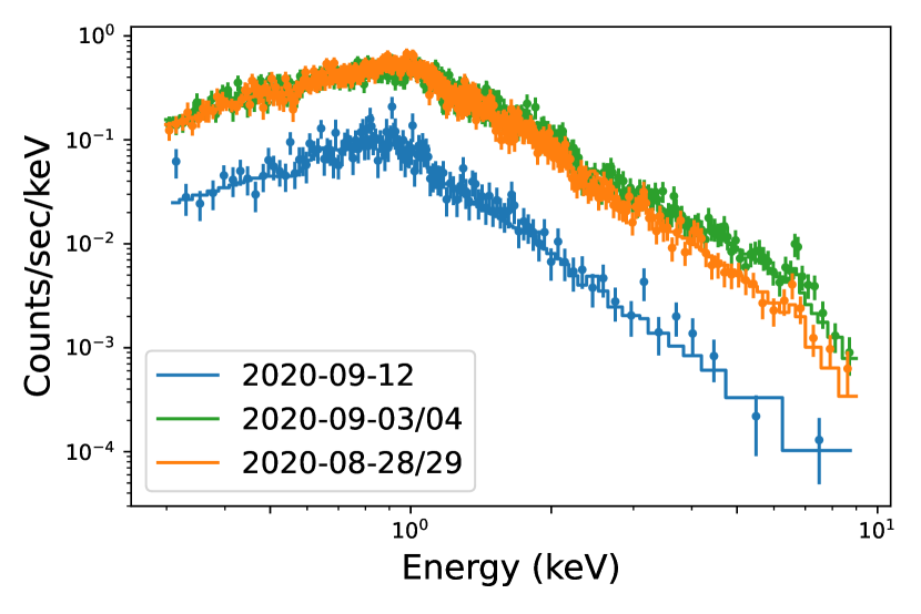
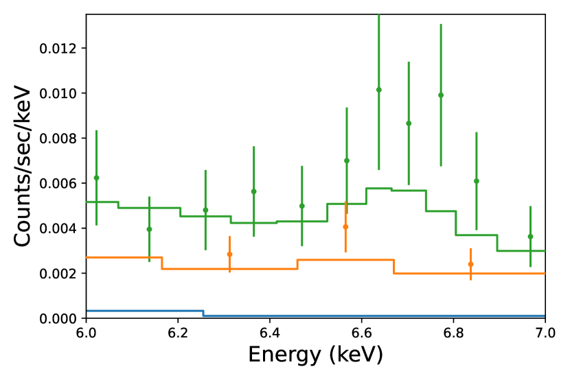
Figure 5: Spectrum of one quiescent observation with XMM-Newton (blue), in comparison to the two observations with flares (orange and green). Left: The two flare spectra exhibit enhancement in overall brightness, and show the Fe 6.7 keV emission line. Right: A detailed look at the 6-7 keV range shows that the Fe 6.7 keV line exhibited by the flare spectra is underfit by models, and that flare spectra show no significant evidence for emission from the fluorescent Fe line at 6.4 keV.

3.5 Time-resolved Spectra of X-ray Flares

Franciosini et al. (2007) present a time-resolved spectroscopic analysis of an observation of XZ Tau AB originally presented in Favata et al. (2003) and reanalyzed in Giardino et al. (2006). In this observation, XZ Tau AB monotonically rises over the course of the $\sim 55$ ks observation. By contrast, in obsid 0865040401 (hereafter referred to as 401), XZ Tau AB monotonically decays, and in observation 0865040601 (hereafter referred to as 601), it exhibits a sharp rise and then decay. The short timescales involved indicate that these are typical flares, rather than long time-scale increases in X-ray brightness associated with magnetic reconnection flares in FUor/EXor outbursts (Kastner et al., 2004).

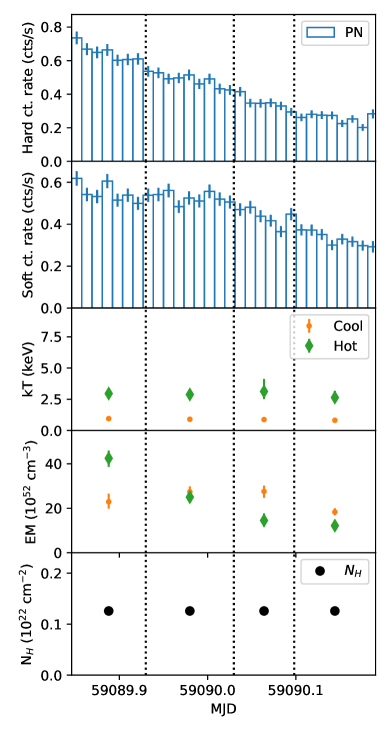
Figure 8: Evolution of XZ Tau AB over the course of a flare decay in observation 0865040401. The decrease in the emission measure of the “hot” component over time clearly tracks the decrease in count rate for photons at energies $>1$ keV, while the temperature of the “hot” component remains stable.

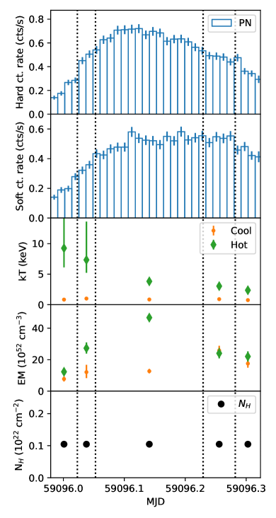
Figure 9: Evolution of XZ Tau AB over the course of a flare rise and decay in observation 0865040601. The change in the emission measure of the “hot” component over time clearly tracks the rise in count rate for photons at energies $>1$ keV. The “cool” component stays fairly stable over time, indicating that most of the change in brightness is due to the hot component.

Following the technique of Franciosini et al. (2007), we divide observations 401 and 601 each into blocks of time using the bayesian_blocks method as provided in AstroPy, and fit models to the spectra from each of these blocks of time to better understand the flare evolution. We assume in these fits that (a) the Ne and Fe-like abundances match those jointly fit to the quiescent observations, and that (b) the hydrogen column density does not change over the course of one observation (i.e. it remains fixed at the best-fit value from fitting the spectrum of the full-duration observation). We present the best-fit parameters in Table 4, and plot the evolution in parameters as a function of time along with the observation light curves in Figures 8 and 9. We discuss the evolution of the flares observed in these observations in more detail in Section 4.2.

3.6 Gratings Data

The combined first (positive and negative) order gratings data from both the High-Energy and Medium-Energy Gratings (HEG and MEG, respectively) from the eleven Chandra observations are presented in Figure 6. We do not consider gratings data from XMM-Newton, due to the likely blend of data in the RGS from XZ Tau AB and the nearby (separation $\sim 12^{\prime\prime}$) HL Tau. Following the method presented in Pradhan et al. (2021), we fit the Chandra grating spectra with a two-temperature model as obtained from XMM-Newton fits, while allowing the spectral parameters to vary over the range allowed by XMM-Newton and fixing the abundances to the XMM-Newton values. We then fit the individual regions line-by-line, grouping the Si XIII, Mg XII, Mg XI, Ne X, Ne IX by a factor of 2. We list our line fluxes for the gratings data in Table 3. Due to the low signal in the Mg XI and Ne IX triplet features, lines typically used to differentiate low-density coronal plasma from high-density plasma associated with accretion shocks, we are unable to constrain the plasma density.

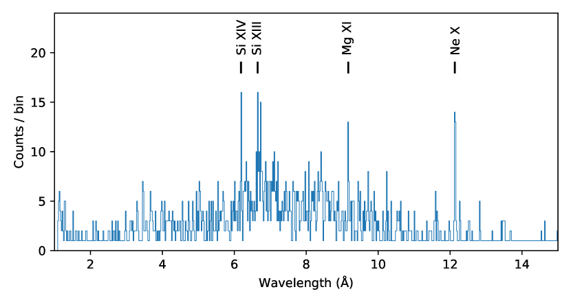
Figure 6: Chandra/HETG data for XZ Tau AB, combining both the MEG and HEG. Prominent lines in the spectrum are labeled. We exclude the spectrum at wavelengths longer than 15 Åas there is minimal emission at these wavelengths due to the contamination of the ACIS-S chip.

Table 3: Line Fluxes from HETGS Spectrum of XZ Tau

	Wavelength	Flux
Line	(Å)	($10^{-7}$ photons cm-2 s-1)
Si XIII (r)	6.648	$3^{+3}_{-2}$
Si XIII (i)	6.687	$<3.36$
Si XIII (f)	6.740	$3^{+2}_{-2}$
Mg XII	8.422	$<3.63$
Mg XI (r)	9.169	$9^{+5}_{-4}$
Mg XI (i)	9.230	$<2.13$
Mg XI (f)	9.314	$3^{+4}_{-3}$
Ne X	12.135	$50^{+21}_{-17}$
Ne IX (r)	13.447	$<29.7$
Fe XIX	13.462	$28^{+33}_{-22}$
Fe XIX	13.518	$14^{+24}_{-7}$
Ne IX (i)	13.552	$<18.1$
Fe XIX	13.645	$<27.7$
Ne IX (f)	13.699	$17^{+24}_{-13}$
Fe XX	13.767	$<1.32$
Fe XVII	13.825	$<2.16$

4 Discussion

4.1 X-ray Evolution Over Time, Or Lack Thereof

We present the best-fit temperatures, emission measures, and abundances for each observation in Table 5. We note that within uncertainties the two components exhibit remarkable consistency in temperature over time. The cool component in particular shows little variation in temperature. The hot component exhibits significantly more uncertainty in each observation, such that while the best-fit temperatures can differ by $\sim 1\mathrm{\;keV}$, the temperatures are generally consistent with each other within the uncertainties. The significant variation in brightness during flares appears to come solely from the emission measure itself, which exhibits moderate increase in the cool component during a flare and an increase on order $\sim 30$ in the hot component. This is generally consistent with a model of occasional flares superposed on top of a stable underlying stellar corona.

To consider the hypothesis of a stable underlying stellar corona, we compare our models to those of previous work analyzing X-ray spectra from XZ Tau AB. We present our results and previous work as a function of time in Figure 7, and briefly discuss the relevant parameters below. The parameters from previous work are summarized in the Appendix.

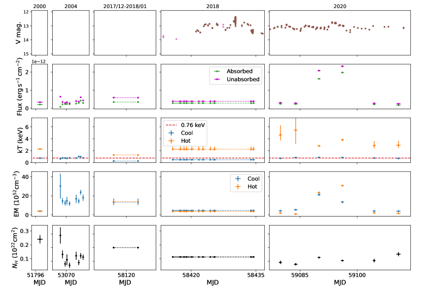
Figure 7: Characteristics of best-fit models to various observations of XZ Tau AB over time, from published work and analysis of unpublished publicly-available data. Rows display (top to bottom) optical brightness as represented by $V$ magnitude, X-ray flux (absorbed and unabsorbed), plasma temperatures, plasma emission measures, and $N_{H}$. Each column spans one set of observations, from 2000 (Güdel et al., 2007), 2004 (Giardino et al., 2006), 2017-2018 (Skinner & Güdel, 2020), 2018, and 2020. Dotted lines connect points representing obsids that were jointly fit.

Skinner & Güdel (2020) jointly fit their two observations of XZ Tau AB in 2017 December and 2018 January with a two-component model with a fixed hydrogen column density of $N_{H}=0.2\mathrm{cm^{2}}$. They find best-fit model temperatures that are quite cool (0.23 keV and 1.28 keV, respectively) compared to those we find. Skinner & Güdel (2020) also present a norm-weighted average temperature of these two components of 0.78 keV, consistent with our cool temperature, and the normalizations of those two components are similarly consistent. This indicates to us that the two-component model they adopt is essentially reproducing our cool component. Similarly, with carefully chosen initial parameters for fitting our data, we can produce a fit to our faint XMM-Newton data with similar (though somewhat worse) goodness-of-fit with temperatures similar to the temperatures found in this work. We thus conclude that the two temperatures found by Skinner & Güdel (2020) reproduce our cool component.

Güdel et al. (2007) present multiple fit options to all sources in the XMM-Newton Extended Survey of the Taurus Molecular Cloud (XEST), including a two-temperature plasma model similar to the parameterization we adopt. They present a fit to the “characteristic” non-flare interval in the data (also analyzed in Favata et al., 2003; Giardino et al., 2006), with best-fit temperatures of $\mathrm{kT_{1}}=0.75$ keV and $\mathrm{kT_{2}}=2.28$ keV, respectively, with emission measures $\mathrm{EM_{1}}=4.00\times 10^{52}\mathrm{cm}^{-3}$ and $\mathrm{EM_{2}}=3.76\times 10^{52}\mathrm{cm}^{-3}$, and a hydrogen column density of $N_{H}=0.24\pm 0.03\times 10^{22}\mathrm{cm^{2}}$. Franciosini et al. (2007) split the observation used for XZ Tau AB in Güdel et al. (2007) into five time-resolved spectra using the Bayesian blocks method and fit a two-temperature plasma to each of these. In this paradigm, the brightening of the light curve corresponded to an increase in the emission measure of the hot plasma, while the cool component held at constant temperature and (until the last spectrum) emission measure. These data directly correspond to our fits despite differences in the treatment of abundance. While Favata et al. (2003) identify a significant decrease in emission measure of the cool component for this observation, Giardino et al. (2006) note that this is due to the spurious elevated $N_{\mathrm{H}}$ level in the first time bin of the time-resolved analysis. Table 4 in Giardino et al. (2006) (which supersedes the Table in Favata et al., 2003) shows that while the emission measure does increase, this increase is not statistically significant. We find that our variability is consistent with the variability summary in Favata et al. (2003) as well; our observed fluxes fall neatly in the range of observed fluxes in this older data.

Giardino et al. (2006) present five days of monitoring of a field that includes XZ Tau AB with XMM-Newton, during a period of high background for the telescope. They present single-temperature fits to these data, finding a stable plasma (albeit with changing hydrogen column density) at a temperature between 0.63 keV and 0.8 keV. Fits to two of their observations indicate a hotter temperature; however, these also show an increase in the observed flux, suggesting a flare. Indeed, the authors note that some of these observations are better fit by a two-component model. We argue that this too demonstrates the persistence of a cool component between 0.7 keV and 0.8 keV over time. We also note that while Giardino et al. (2006) hypothesize that the change in the XZ Tau AB X-ray spectrum is connected to the end of XZ Tau B’s outburst, we find that the spectrum remains similar to the 2004 result despite the apparent outburst of XZ Tau B during our observations.

From these data, we see that both in the raw observables and in the adopted modeling paradigm of stellar X-ray spectra as stacked single-temperature plasmas, XZ Tau AB remains fairly stable over observations spanning the 2000-2020 timeframe, with the few exceptions of likely flares, as shown in Figure 7. Observed fluxes remain fairly stable over time apart from the observations we identify as flares. $N_{H}$ varies around a consistently low level, indicating that the observations (particularly recent Chandra observations with limited sensitivity to soft X-rays) do not have much leverage to constrain $N_{H}$. The best-fit models consistently exhibit a cool temperature between 0.7-0.8 keV, indicating a stable temperature feature we interpret as the stellar corona(e). Due to different models assumptions (e.g. abundances), the emission measures and $N_{\mathrm{H}}$ vary widely for different datasets and are not directly comparable. The ratio of temperature components and variability within each set are robust, as can be seen in the flares in 2020. The consistency of the cool component over an interval of twenty years bolsters our hypothesis of an underlying stable corona, with occasional flares superposed on top of this, and recommends against the idea that flares completely reorganize the stellar coronal behavior.

Table 4: Summary of parameters for best fit models for time-resolved spectra of XZ Tau AB Flares

		$N_{H}$	Cool Component		Hot Component		Flux ($10^{-13}\mathrm{erg\,s^{-1}\,cm^{-2}}$)		Log(Lum.)
obsid	rstat	($10^{22}\mathrm{cm}^{-2}$)	kT (keV)	EM ($10^{52}\mathrm{cm}^{-3}$)	kT (keV)	EM ($10^{52}\mathrm{cm}^{-3}$)	Absorbed	Unabsorbed	log (erg $\mathrm{s}^{-1}$)
FaintXMM	0.9135	$0.113_{-0.007}^{+0.007}$	$0.75_{-0.02}^{+0.02}$	$4.3_{-0.2}^{+0.2}$	$3.2_{-0.3}^{+0.5}$	$1.7_{-0.2}^{+0.2}$	2.078	2.739	29.8
0865040401A	0.5724	$0.127$	$0.95_{-0.05}^{+0.06}$	$21_{-3}^{+3}$	$3.0_{-0.2}^{+0.3}$	$39_{-3}^{+3}$	23.98	28.71	30.8
0865040401B	0.7251	$0.127$	$0.89_{-0.04}^{+0.04}$	$25_{-2}^{+2}$	$2.9_{-0.3}^{+0.4}$	$23_{-2}^{+2}$	17.92	22.08	30.7
0865040401C	0.5207	$0.127$	$0.87_{-0.04}^{+0.04}$	$25_{-3}^{+2}$	$3.1_{-0.6}^{+1.0}$	$13_{-3}^{+3}$	13.92	17.49	30.6
0865040401D	0.6073	$0.127$	$0.81_{-0.03}^{+0.04}$	$17_{-1}^{+2}$	$2.6_{-0.4}^{+0.5}$	$11_{-2}^{+2}$	9.909	12.54	30.5
0865040601A	0.5601	$0.105$	$0.82_{-0.12}^{+0.10}$	$7_{-1}^{+1}$	$9_{-3}^{+9}$	$11_{-1}^{+1}$	9.291	10.73	30.4
0865040601B	0.6247	$0.105$	$0.99_{-0.15}^{+0.14}$	$11_{-3}^{+4}$	$7_{-2}^{+6}$	$25_{-3}^{+3}$	18.65	21.23	30.7
0865040601C	0.6304	$0.105$	$0.84_{-0.05}^{+0.05}$	$12_{-1}^{+1}$	$3.8_{-0.2}^{+0.2}$	$42_{-1}^{+1}$	25.03	29.13	30.8
0865040601D	0.7071	$0.105$	$0.89_{-0.05}^{+0.05}$	$23_{-3}^{+3}$	$3.0_{-0.4}^{+0.6}$	$22_{-3}^{+3}$	17.32	21.27	30.7
0865040601E	0.591	$0.105$	$0.74_{-0.07}^{+0.06}$	$16_{-2}^{+2}$	$2.4_{-0.4}^{+0.5}$	$20_{-3}^{+3}$	13.07	16.38	30.6

4.2 Short-term Coronal Variability

Observation 401 shows the clear signatures of the decay phase of a flare. The hardness of the spectrum evolves over time–the count rates clearly show a decrease in hard flux while soft flux remains stable over the first two blocks of time (before roughly MJD 59090.03), before the soft flux also begins to decay over the latter half of the observation. The best-fit temperatures, abundances, and hydrogen column densities remain stable across the observation, though there is substantial uncertainty in the temperature of the hot component in the third, shortest, block of time. The clearest change over time is in the emission measures of the “hot” component, which we will refer to in this section as the flare component. The flare component’s emission measure decreases by $>60\%$ between the first and fourth blocks, while the emission measure of the cool component stays stable (within uncertainties) over that time frame. This indicates that for this flare, the decay is solely driven by the emission measure decreasing. It is notable that the emission measures invert in the third block of time, albeit with substantial uncertainties.

Observation 601, on the other hand, shows both the rise and the start of the decay for the flare, and the characteristics are not nearly as clear-cut as in 401. Qualitatively, as the hard flux peaks the soft flux levels off, leading to a decay phase similar to that seen in 401. The increase in hard flux is steeper than in the soft, as there is less hard flux initially and more hard flux at the peak.

While the cool component maintains its characteristic behavior (albeit with substantial uncertainties) throughout the flare, the hot component is far more variable. During the rise phase, the temperature is elevated compared to both 401 and the decay phase of this flare, while the emission measure increases, suggesting a hotter plasma in the rise than in the decay.

The detection of the flare peak in observation 601 allows for a fuller characterization of the coronal loops produced by the flare based on the flare decay. Following the application of Reale et al. (2004) by Giardino et al. (2006) and Franciosini et al. (2007), we estimate the flare loop semi-length $L$ from the $e$-folding timescale of the decay and the maximum temperatures $T_{\mathrm{max}}$ via the equation

$$L=\frac{\tau_{\mathrm{LC}}\sqrt{T_{\mathrm{max}}}}{\alpha F(\zeta)},$$ (1)

where $\alpha=3.7\times 10^{-4}\mathrm{cm^{-1}\,s^{-1}\,K^{1/2}}$, $\tau_{\mathrm{LC}}$ is the $e$-folding timescale of the decay, and $T_{\mathrm{max}}$ is the maximum plasma temperature of the flare, while accounting for heating during the decay via $\zeta$, the slope of the flare decay in the $\log(T)$ vs. $\log(\sqrt{EM})$ plane, shown in Figure 10.

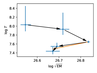
Figure 10: $\log(T)$ of the five time-resolved spectra of Observation 601, as a function of $\log(\sqrt{EM})$. Arrows indicate the time order of observations. The orange line reflects the slope $\zeta$ of the flare decay in this space.

These characteristics (including the relationship between the best-fit peak temperature $T_{\mathrm{obs}}$ and $T_{\mathrm{max}}$) are calibrated for the PN detector; however, Franciosini et al. (2007) found that these formulae would give order-of-magnitude results for the MOS detectors as well, given the similarities of the instruments and the width of the adopted spectral band. We thus use these equations for our temperatures and emission measures derived from joint fits to the three detectors.

For the flare in 601, we find $\zeta=1.2\pm 0.4$. We find an $e$-folding timescale based on fitting a line to the natural logarithm of the decay phase light curve of $50\pm 4$ ks. The best-fit maximum temperature $T_{\mathrm{obs}}=44_{-2}^{+3}$ MK, which following Equation (3) from Giardino et al. (2006) corresponds to a maximum temperature of $T_{\mathrm{max}}=96^{+4}_{-3}$ MK. Inputting this information into Equation 1 yields a loop length of $\sim 10R_{\odot}$, corresponding to $\sim 6R_{\star}$ for XZ Tau A and $\sim 9R_{\star}$ for XZ Tau B. These lengths are such that the flare could reach into the disk, though we do not have direct measurement of the inner disk radius for either star; ALMA data do not resolve the dust emission for either disk and thus leave the radius as $\lesssim 15$ au (Ichikawa et al., 2021). Such extended flare sizes are not uncommon in pre-main sequence disk-hosting stars (e.g. Favata et al., 2005); however, there is no apparent difference in flare energy or flare peak energy between flares on disk-hosting and diskless pre-main sequence stars (Getman & Feigelson, 2021), and further work suggests that flares in disk-hosting pre-main sequence stars also exhibit loops with both footprints in the stellar surface, rather than a flare that extends from star to disk (Getman et al., 2021). The data in hand do not make it more or less likely that either star produced the flare, in our opinion; while XZ Tau B is thought to be an ExOR object, both XZ Tau A and B are young stars with disks, making flare events likely from both.

We also attempted using the available data from the flare during observation 401 to provide a lower limit for the coronal loops in that flare as well. For that flare, we find a lower limit decay $e$-folding time of $33\pm 1$ ks and a lower limit maximum temperature of $72_{-4}^{+5}$ MK. However, for this flare $\zeta\sim$ 0.1, well below the validity threshold for the relation of $0.35<\zeta\leq 1.6$.

4.3 A YSO Coronal Spectrum Over Time Looks like a Snapshot of a Young Cluster

Many studies of young stars, such as the Chandra Orion Ultradeep Project (COUP; Getman et al., 2005), and the XMM-Newton Extended Survey of Taurus (XEST; Güdel et al., 2007), look at entire young clusters, leveraging the ability to study many YSOs at once rather than focusing on a single source. Because of the multiple observations of XZ Tau AB over time discussed in Section 4.1, we can compare the ensemble of states of XZ Tau AB over time against other studies which have taken snapshots of an entire cluster at a given point in time.

To test this, we compared the temperatures and emission measures of our models of XZ Tau AB and those from previous work as a function of X-ray luminosity against the same characteristics for a subset of the data from COUP with two-temperature models that produce good fits (i.e. not meeting the “marginal” or “poor” flags in their paper), following the comparison of Preibisch et al. (2005) with the initial COUP dataset.

As seen in Figure 11, the XZ Tau AB data traces across the scatter in the COUP dataset. While the cool temperature component does stay steady as a function of unabsorbed X-ray luminosity, the hot component increases in temperature as a function of luminosity for both the COUP dataset and XZ Tau AB, an expected result of flare activity. XZ Tau AB over time similarly follows the trend across the COUP snapshot of increasing ratio of hot emission measure to cool as a function of X-ray luminosity (albeit with a fair amount of scatter). This suggests to us the possibility that much of the observed variation in the X-ray characteristics of YSOs is due primarily to the chance timing of the observation, rather than to fundamental differences in the stars themselves.

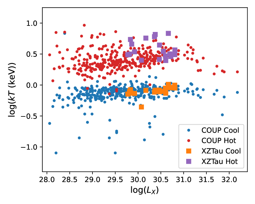
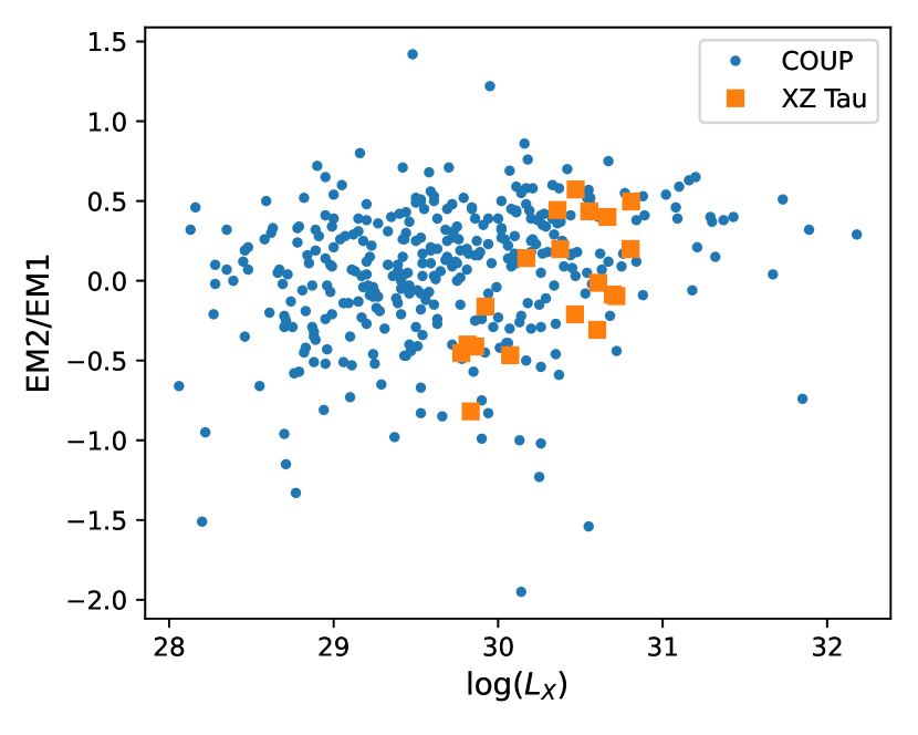
Figure 11: Comparison of models of various observations of XZ Tau AB over time to model fits to the Chandra Orion Ultradeep Project (COUP). Left: As with COUP model fits, XZ Tau AB over time exhibits a steady cool component and variable hot component that increase in brightness with increasing absorption-corrected X-ray luminosity. Right: As with COUP model fits, the ratio of emission measures of warm and cool components increases (i.e. the warm component increases in emission) as a function of absorption-corrected X-ray luminosity.

5 Summary

In this paper, we present CCD-resolution and gratings spectra of the pre-main sequence binary system XZ Tau AB from both Chandra and XMM-Newton. We find the following.

• The Chandra and XMM-Newton data are both consistent with a two-temperature plasma-emission model.

• The cool component of the two-temperature model remains stable across both the Chandra and XMM-Newton observations, and is consistent with previous observations of the system with both observatories spanning more than a decade. This suggests a rotationally-induced magnetic field corona that remains stable over this timeframe, with recurring aperiodic flare activity superposed on top of this stable feature.

• The scatter in model fits of XZ Tau AB over time is comparable to the scatter in two-component model fits of the sources in COUP.

• Time-resolved spectra of two flares observed with XMM-Newton show that the primary change during the flare is an increase in the volume emission measure of the “hot” component. Detailed analysis of the decay of one flare indicated a plasma loop length of $\sim 10R_{\odot}$.

• XZ Tau AB is likely undergoing a long-term outburst typical of EXor objects during our X-ray observations based on the optical light curves. However, the change in X-ray brightness we see during several observations is more consistent with short-duration coronal flares than the long-term X-ray brightness increase seen in other EXOr objects (e.g. V1647 Ori; Hamaguchi et al., 2012).

Appendix A Fitting New Chandra and XMM-Newton Data with Variable Abundances

While we adopt the case that the Ne and Fe abundances are not significantly varying over the timeframe of our observations, we present here our best-fit models for these data, with Ne and Fe allowed to vary, for comparison.

=6.5cm

Table 5: Summary of parameters for best fit models for X-ray spectra of XZ Tau AB with freely-varying Ne and Fe-like abundances

		$N_{H}$	Cool Component				Hot Component		Flux ($10^{-13}\,\mathrm{ergs^{-1}\,cm^{-2}}$)		Log(Lum.)
obsid	rstat	($10^{22}\mathrm{cm}^{-2}$)	kT (keV)	EM $10^{52}\mathrm{cm}^{-3}$	Ne ($\mathrm{Ne_{\odot}}$)	Fe ($\mathrm{Fe_{\odot}}$)	kT (keV)	EM ($10^{52}\mathrm{cm}^{-3}$)	Absorbed	Unabsorbed	log (erg $\mathrm{s}^{-1}$)
All Chandra	$0.568$	$0.11$	$0.83_{-0.6}^{+0.1}$	$1.0_{-0.4}^{+0.6}$	$7.6_{-4.2}^{+4.8}$	$0.9_{-0.3}^{+0.4}$	$2.2_{-0.2}^{+0.2}$	$3.0_{-0.4}^{+1.3}$	$2.5$	$3.1$	29.9
201610	$0.378$	$0.11$	$0.29_{-0.3}^{+1}$	$15_{-14}^{+649}$	$0.6_{-0.6}^{+31.6}$	$0.9_{-0.9}^{+7.8}$	$3.2_{-1.1}^{+nan}$	$4_{-3}^{+2}$	$7.4$	$11.6$	30.5
219510	$0.131$	$0.11$	$0.73_{-0.7}^{+0.5}$	$8_{-7}^{+22}$	$2.6_{-2.6}^{+8.0}$	$0.2_{-0.2}^{+0.9}$	$2.55_{nan}^{+nan}$	$6_{-5}^{+7}$	$5.7$	$7.5$	30.3
Faint Chandra	$0.769$	$0.11$	$0.39_{-0.2}^{+0.8}$	$0.5_{-0.3}^{+0.6}$	$7.4_{-3.8}^{+7.6}$	$1.0_{-0.4}^{+0.7}$	$1.8_{-0.2}^{+0.2}$	$2.6_{-0.6}^{+0.6}$	$1.9$	$2.4$	29.8
Faint XMM-Newton	$0.915$	$0.11_{-0.01}^{+0.01}$	$0.75_{-0.02}^{+0.02}$	$4.7_{-0.6}^{+0.6}$	$1.4_{-0.2}^{+0.2}$	$0.11_{-0.01}^{+0.02}$	$3.2_{-0.4}^{+0.7}$	$1.9_{-0.3}^{+0.3}$	$2.1$	$2.7$	29.9
0865040201	$0.61$	$0.10_{-0.02}^{+0.02}$	$0.74_{-0.05}^{+0.04}$	$5.1_{-1.0}^{+1.2}$	$1.3_{-0.3}^{+0.3}$	$0.10_{-0.02}^{+0.03}$	$5.0_{-1.2}^{+3.8}$	$2.1_{-0.5}^{+0.4}$	$2.5$	$3.1$	29.9
0865040301	$0.573$	$0.08_{-0.01}^{+0.01}$	$0.80_{-0.05}^{+0.05}$	$6.1_{-1.2}^{+1.1}$	$1.6_{-0.3}^{+0.4}$	$0.09_{-0.02}^{+0.02}$	$5.5_{-2.6}^{+nan}$	$1.0_{-0.4}^{+0.6}$	$2.3$	$2.9$	29.9
0865040401	$0.716$	$0.10_{-0.01}^{+0.01}$	$0.85_{-0.02}^{+0.03}$	$10.3_{-1.3}^{+1.6}$	$1.8_{-0.3}^{+0.3}$	$0.26_{-0.03}^{+0.04}$	$2.44_{-0.09}^{+0.08}$	$30.4_{-0.8}^{+0.9}$	$16.3$	$19.6$	30.7
0865040601	$0.684$	$0.08_{-0.01}^{+0.01}$	$0.78_{-0.04}^{+0.03}$	$6.0_{-0.9}^{+1.2}$	$2.6_{-0.4}^{+0.4}$	$0.26_{-0.04}^{+0.04}$	$3.5_{-0.1}^{+0.1}$	$35.8_{-0.8}^{+0.8}$	$19.8$	$22.5$	30.8
0865040701	$0.688$	$0.10_{-0.02}^{+0.02}$	$0.79_{-0.05}^{+0.05}$	$4.2_{-1.3}^{+1.5}$	$1.1_{-0.4}^{+0.5}$	$0.13_{-0.03}^{+0.05}$	$2.7_{-0.5}^{+1.1}$	$2.3_{-0.7}^{+0.6}$	$2.1$	$2.7$	29.8
0865040501	$0.619$	$0.15_{-0.02}^{+0.02}$	$0.71_{-0.05}^{+0.04}$	$4.2_{-1.1}^{+1.1}$	$1.3_{-0.3}^{+0.4}$	$0.12_{-0.02}^{+0.04}$	$2.9_{-0.5}^{+0.9}$	$1.8_{-0.4}^{+0.4}$	$1.7$	$2.5$	29.8

Appendix B Summary of Parameters from Previous Observations

We compiled fit parameters for previous observations of XZ Tau from Güdel et al. (2007); Franciosini et al. (2007); Giardino et al. (2006); Skinner & Güdel (2020), in addition to our analysis here. While the methodologies between each paper are different enough to not be directly comparable on a numerical basis (e.g. different treatments of metallicity), they provide the backbone for the comparison presented in Figure 7.

Table 6: Comparison of Present Work to Previous Observations

	Abundance			Fit Boundsb	$N_{H}\,^{c}$	kT (keV)		EM ($10^{52}\,\mathrm{{cm}^{-3}}$)		Flux ($10^{-13}\mathrm{erg\,cm^{-2}\,s^{-1}}$)
Source	Type	Uncertaintya	Year	(keV)	($10^{22}\mathrm{cm^{-2}}$)	Cool	Hot	Cool	Hot	Absorbed	Unabsorbed
XEST	(1)	0.68	2000	0.5 - 7.3	$0.24_{-0.03}^{+0.03}$	$0.7497$	$2.278$	$4$	$3.76$	$2.078$	$3.38$
FranciosiniA	(1)	0.9	2000	0.3 - 7.3	$0.245_{-0.044}^{+0.061}$	$0.73_{-0.11}^{+0.08}$	$3.44_{-0.95}^{+2.31}$	$4.5_{-0.9}^{+1.2}$	$3.1_{-0.7}^{+0.9}$	$2.217$	$3.567$
FranciosiniB	(1)	0.9	2000	0.3 - 7.3	$0.205_{-0.039}^{+0.047}$	$0.82_{-0.09}^{+0.15}$	$5.72_{-1.71}^{+4.49}$	$4.9_{-1.2}^{+1.6}$	$6.8_{-0.9}^{+1.2}$	$4.735$	$6.324$
FranciosiniC	(1)	0.9	2000	0.3 - 7.3	$0.191_{-0.033}^{+0.039}$	$0.77_{-0.12}^{+0.13}$	$6.03_{-1.51}^{+2.06}$	$4.5_{-1.4}^{+1.4}$	$12.5_{-0.9}^{+1.6}$	$7.775$	$9.783$
FranciosiniD	(1)	0.9	2000	0.3 - 7.3	$0.222_{-0.021}^{+0.023}$	$0.78_{-0.09}^{+0.13}$	$4.42_{-0.45}^{+0.64}$	$4.9_{-1.2}^{+1.2}$	$18.3_{-1.2}^{+1.2}$	$9.662$	$12.63$
FranciosiniE	(1)	0.9	2000	0.3 - 7.3	$0.256_{-0.026}^{+0.029}$	$0.79_{-0.09}^{+0.09}$	$3.5_{-0.42}^{+0.52}$	$8.2_{-1.9}^{+1.9}$	$22.3_{-1.6}^{+2.1}$	$10.82$	$15.29$
Giardino201	(2)	0.68	2004	0.3 - 7.5	$0.29_{-0.06}^{+0.06}$	$0.63_{-0.06}^{+0.06}$	$\cdots$	$30.2_{-13.1}^{+13.1}$	$\cdots$	$0.7543$	$6.388$
Giardino301	(2)	0.68	2004	0.3 - 7.3	$0.15_{-0.03}^{+0.03}$	$0.78_{-0.04}^{+0.04}$	$\cdots$	$14.6_{-3.2}^{+3.2}$	$\cdots$	$2.215$	$3.465$
Giardino401	(2)	0.68	2004	0.3 - 7.3	$0.08_{-0.02}^{+0.02}$	$0.77_{-0.04}^{+0.04}$	$\cdots$	$12.5_{-2.6}^{+2.6}$	$\cdots$	$2.294$	$2.952$
Giardino501	(2)	0.68	2004	0.3 - 7.3	$0.11_{-0.04}^{+0.04}$	$0.72_{-0.05}^{+0.05}$	$\cdots$	$14.7_{-4.1}^{+4.1}$	$\cdots$	$2.362$	$3.364$
Giardino601	(2)	0.68	2004	0.3 - 7.3	$0.07_{-0.02}^{+0.02}$	$0.78_{-0.04}^{+0.04}$	$\cdots$	$11.9_{-5.2}^{+0.4}$	$\cdots$	$2.265$	$2.824$
Giardino901	(2)	0.68	2004	0.3 - 7.3	$0.14_{-0.03}^{+0.03}$	$0.76_{-0.05}^{+0.05}$	$\cdots$	$16.8_{-4.4}^{+4.4}$	$\cdots$	$2.572$	$3.944$
Giardino1001	(2)	0.68	2004	0.3 - 7.3	$0.09_{-0.02}^{+0.02}$	$1.03_{-0.07}^{+0.07}$	$\cdots$	$14.5_{-2.6}^{+2.6}$	$\cdots$	$2.948$	$3.723$
Giardino1101	(2)	0.68	2004	0.3 - 7.3	$0.14_{-0.02}^{+0.02}$	$1.00_{-0.04}^{+0.04}$	$\cdots$	$23.7_{-2.5}^{+2.5}$	$\cdots$	$4.240$	$6.046$
Giardino1201	(2)	0.68	2004	0.3 - 7.3	$0.13_{-0.02}^{+0.02}$	$0.80_{-0.04}^{+0.04}$	$\cdots$	$18_{-3.3}^{+3.3}$	$\cdots$	$2.931$	$4.315$
Skinner	(3)	0.68	2017	0.3 - 8	$0.2$	$0.26_{-0.03}^{+0.04}$	$1.28_{-0.04}^{+0.04}$	$13.37_{-3.049}^{+3.752}$	$13.84_{-0.9381}^{+0.9381}$	$3.446$	$5.895$
ChandraFull	(4)	0.68	2018	0.5 - 8	$0.113$	$0.49_{-0.05}^{+0.10}$	$2.3_{-0.3}^{+0.4}$	$4.6_{-0.6}^{+0.7}$	$3.6_{-0.7}^{+0.5}$	$2.837$	$3.862$
FaintXMM	(5)	0.68	2020	0.3 - 9	$0.113_{-0.007}^{+0.007}$	$0.75_{-0.02}^{+0.02}$	$3.2_{-0.3}^{+0.5}$	$4.3_{-0.2}^{+0.2}$	$1.7_{-0.2}^{+0.2}$	$2.078$	$2.739$
0865040201	(4)	0.68	2020	0.3 - 9	$0.09_{-0.01}^{+0.01}$	$0.72_{-0.04}^{+0.04}$	$4.6_{-0.9}^{+1.6}$	$4.3_{-0.3}^{+0.3}$	$2.0_{-0.3}^{+0.3}$	$2.477$	$3.06$
0865040301	(4)	0.68	2020	0.3 - 9	$0.077_{-0.009}^{+0.009}$	$0.84_{-0.03}^{+0.03}$	$5_{-2}^{+14}$	$5.4_{-0.4}^{+0.3}$	$0.9_{-0.2}^{+0.3}$	$2.326$	$2.831$
0865040401	(4)	0.68	2020	0.3 - 9	$0.127_{-0.005}^{+0.005}$	$0.87_{-0.02}^{+0.02}$	$2.8_{-0.1}^{+0.2}$	$21_{-1}^{+1}$	$23_{-1}^{+1}$	$16.31$	$20.84$
0865040401A	(4)	0.68	2020	0.3 - 9	$0.127$	$0.95_{-0.05}^{+0.06}$	$3.0_{-0.2}^{+0.3}$	$21_{-3}^{+3}$	$39_{-3}^{+3}$	$23.98$	$28.71$
0865040401B	(4)	0.68	2020	0.3 - 9	$0.127$	$0.89_{-0.04}^{+0.04}$	$2.9_{-0.3}^{+0.4}$	$25_{-2}^{+2}$	$23_{-2}^{+2}$	$17.92$	$22.08$
0865040401C	(4)	0.68	2020	0.3 - 9	$0.127$	$0.87_{-0.04}^{+0.04}$	$3.1_{-0.6}^{+1}$	$25_{-3}^{+2}$	$13_{-3}^{+3}$	$13.92$	$17.49$
0865040401D	(4)	0.68	2020	0.3 - 9	$0.127$	$0.81_{-0.03}^{+0.04}$	$2.6_{-0.4}^{+0.5}$	$17_{-1}^{+2}$	$11_{-2}^{+2}$	$9.909$	$12.54$
0865040601	(4)	0.68	2020	0.3 - 9	$0.105_{-0.005}^{+0.005}$	$0.85_{-0.03}^{+0.03}$	$3.8_{-0.2}^{+0.2}$	$13.4_{-0.8}^{+0.8}$	$31_{-1}^{+1}$	$19.76$	$23.27$
0865040601A	(4)	0.68	2020	0.3 - 9	$0.105$	$0.82_{-0.12}^{+0.10}$	$9_{-3}^{+9}$	$7_{-1}^{+1}$	$11_{-1}^{+1}$	$9.291$	$10.73$
0865040601B	(4)	0.68	2020	0.3 - 9	$0.105$	$0.99_{-0.15}^{+0.14}$	$7_{-2}^{+6}$	$11_{-3}^{+4}$	$25_{-3}^{+3}$	$18.65$	$21.23$
0865040601C	(4)	0.68	2020	0.3 - 9	$0.105$	$0.84_{-0.05}^{+0.05}$	$3.8_{-0.2}^{+0.2}$	$12_{-1}^{+1}$	$42_{-1}^{+1}$	$25.03$	$29.13$
0865040601D	(4)	0.68	2020	0.3 - 9	$0.105$	$0.89_{-0.05}^{+0.05}$	$3.0_{-0.4}^{+0.6}$	$23_{-3}^{+3}$	$22_{-3}^{+3}$	$17.32$	$21.27$
0865040601E	(4)	0.68	2020	0.3 - 9	$0.105$	$0.74_{-0.07}^{+0.06}$	$2.4_{-0.4}^{+0.5}$	$16_{-2}^{+2}$	$20_{-3}^{+3}$	$13.07$	$16.38$
0865040701	(4)	0.68	2020	0.3 - 9	$0.10_{-0.01}^{+0.02}$	$0.77_{-0.04}^{+0.04}$	$2.9_{-0.5}^{+0.8}$	$4.0_{-0.4}^{+0.4}$	$2.0_{-0.4}^{+0.3}$	$2.146$	$2.752$
0865040501	(4)	0.68	2020	0.3 - 9	$0.15_{-0.01}^{+0.02}$	$0.71_{-0.04}^{+0.04}$	$2.9_{-0.5}^{+0.7}$	$3.9_{-0.3}^{+0.3}$	$1.6_{-0.3}^{+0.3}$	$1.724$	$2.497$

Note. — (1) Fixed VAPEC model abundances described in Güdel et al. (2007), based on Telleschi et al. (2005), Argiroffi et al. (2004), García-Alvarez et al. (2005), and Scelsi et al. (2005). (2) Fixed metallicity of $Z=0.08Z_{\odot}$ based on average metallicity across fits to eleven individual observations. (3) Best fit metallicity of $Z=0.14_{-0.02}^{+0.03}Z_{\odot}$. (4) Fixed Ne and Fe values based on the best fit to a joint fit of the four XMM-Newton observations not during flares. (5) Best-fit Ne and Fe values for this fit.

(a) Decimal uncertainties—i.e.  0.68 corresponds to 68% uncertainties in the following numbers.

(b) Energy range considered when fitting—i.e. data outside these bounds are not considered in the fit.

(c) Values listed without uncertainties are fixed at the quoted value in the fitting.

References

- Arce & Sargent (2006) Arce, H. G., & Sargent, A. I. 2006, ApJ, 646, 1070, doi: 10.1086/505104
- Argiroffi et al. (2004) Argiroffi, C., Drake, J. J., Maggio, A., et al. 2004, ApJ, 609, 925, doi: 10.1086/420692
- Astropy Collaboration et al. (2013) Astropy Collaboration, Robitaille, T. P., Tollerud, E. J., et al. 2013, A&A, 558, A33, doi: 10.1051/0004-6361/201322068
- Astropy Collaboration et al. (2018) Astropy Collaboration, Price-Whelan, A. M., Sipőcz, B. M., et al. 2018, AJ, 156, 123, doi: 10.3847/1538-3881/aabc4f
- Audard et al. (2014) Audard, M., Ábrahám, P., Dunham, M. M., et al. 2014, in Protostars and Planets VI, ed. H. Beuther, R. S. Klessen, C. P. Dullemond, & T. Henning, 387, doi: 10.2458/azu_uapress_9780816531240-ch017
- Bonito et al. (2007) Bonito, R., Orlando, S., Peres, G., Favata, F., & Rosner, R. 2007, A&A, 462, 645, doi: 10.1051/0004-6361:20065236
- Brickhouse et al. (2010) Brickhouse, N. S., Cranmer, S. R., Dupree, A. K., Luna, G. J. M., & Wolk, S. 2010, ApJ, 710, 1835, doi: 10.1088/0004-637X/710/2/1835
- Canizares et al. (2005) Canizares, C. R., Davis, J. E., Dewey, D., et al. 2005, PASP, 117, 1144, doi: 10.1086/432898
- Clarke et al. (1990) Clarke, C. J., Lin, D. N. C., & Pringle, J. E. 1990, MNRAS, 242, 439, doi: 10.1093/mnras/242.3.439
- Cleeves et al. (2013) Cleeves, L. I., Adams, F. C., & Bergin, E. A. 2013, ApJ, 772, 5, doi: 10.1088/0004-637X/772/1/5
- Coffey et al. (2004) Coffey, D., Downes, T. P., & Ray, T. P. 2004, A&A, 419, 593, doi: 10.1051/0004-6361:20034316
- Favata et al. (2005) Favata, F., Flaccomio, E., Reale, F., et al. 2005, ApJS, 160, 469, doi: 10.1086/432542
- Favata et al. (2002) Favata, F., Fridlund, C. V. M., Micela, G., Sciortino, S., & Kaas, A. A. 2002, A&A, 386, 204, doi: 10.1051/0004-6361:20011387
- Favata et al. (2003) Favata, F., Giardino, G., Micela, G., Sciortino, S., & Damiani, F. 2003, A&A, 403, 187, doi: 10.1051/0004-6361:20030305
- Foster et al. (2012) Foster, A. R., Ji, L., Smith, R. K., & Brickhouse, N. S. 2012, ApJ, 756, 128, doi: 10.1088/0004-637X/756/2/128
- Franciosini et al. (2007) Franciosini, E., Pillitteri, I., Stelzer, B., et al. 2007, A&A, 468, 485, doi: 10.1051/0004-6361:20066536
- Freeman et al. (2001) Freeman, P., Doe, S., & Siemiginowska, A. 2001, in Society of Photo-Optical Instrumentation Engineers (SPIE) Conference Series, Vol. 4477, Astronomical Data Analysis, ed. J.-L. Starck & F. D. Murtagh, 76–87, doi: 10.1117/12.447161
- Fruscione et al. (2006) Fruscione, A., McDowell, J. C., Allen, G. E., et al. 2006, in Society of Photo-Optical Instrumentation Engineers (SPIE) Conference Series, Vol. 6270, Society of Photo-Optical Instrumentation Engineers (SPIE) Conference Series, ed. D. R. Silva & R. E. Doxsey, 62701V, doi: 10.1117/12.671760
- García-Alvarez et al. (2005) García-Alvarez, D., Drake, J. J., Lin, L., Kashyap, V. L., & Ball, B. 2005, ApJ, 621, 1009, doi: 10.1086/427721
- Getman & Feigelson (2021) Getman, K. V., & Feigelson, E. D. 2021, ApJ, 916, 32, doi: 10.3847/1538-4357/ac00be
- Getman et al. (2021) Getman, K. V., Feigelson, E. D., & Garmire, G. P. 2021, ApJ, 920, 154, doi: 10.3847/1538-4357/ac1746
- Getman et al. (2005) Getman, K. V., Flaccomio, E., Broos, P. S., et al. 2005, ApJS, 160, 319, doi: 10.1086/432092
- Giardino et al. (2006) Giardino, G., Favata, F., Silva, B., et al. 2006, A&A, 453, 241, doi: 10.1051/0004-6361:20053663
- Grosso et al. (2006) Grosso, N., Feigelson, E. D., Getman, K. V., et al. 2006, A&A, 448, L29, doi: 10.1051/0004-6361:200600004
- Güdel et al. (2008) Güdel, M., Skinner, S. L., Audard, M., Briggs, K. R., & Cabrit, S. 2008, A&A, 478, 797, doi: 10.1051/0004-6361:20078141
- Güdel et al. (2007) Güdel, M., Briggs, K. R., Arzner, K., et al. 2007, A&A, 468, 353, doi: 10.1051/0004-6361:20065724
- Haas et al. (1990) Haas, M., Leinert, C., & Zinnecker, H. 1990, A&A, 230, L1
- Hamaguchi et al. (2012) Hamaguchi, K., Grosso, N., Kastner, J. H., et al. 2012, ApJ, 754, 32, doi: 10.1088/0004-637X/754/1/32
- Harris et al. (2020) Harris, C. R., Millman, K. J., van der Walt, S. J., et al. 2020, Nature, 585, 357, doi: 10.1038/s41586-020-2649-2
- Huenemoerder et al. (2007) Huenemoerder, D. P., Kastner, J. H., Testa, P., Schulz, N. S., & Weintraub, D. A. 2007, ApJ, 671, 592, doi: 10.1086/522921
- Hunter (2007) Hunter, J. D. 2007, Computing In Science & Engineering, 9, 90, doi: 10.1109/MCSE.2007.55
- Ichikawa et al. (2021) Ichikawa, T., Kido, M., Takaishi, D., et al. 2021, ApJ, 919, 55, doi: 10.3847/1538-4357/ac0dc3
- Jayasinghe et al. (2019) Jayasinghe, T., Stanek, K. Z., Kochanek, C. S., et al. 2019, MNRAS, 486, 1907, doi: 10.1093/mnras/stz844
- Jones et al. (2001) Jones, E., Oliphant, T., Peterson, P., & Others. 2001, SciPy: Open source scientific tools for Python. http://www.scipy.org/
- Kastner et al. (2002) Kastner, J. H., Huenemoerder, D. P., Schulz, N. S., Canizares, C. R., & Weintraub, D. A. 2002, The Astrophysical Journal, 567, 434, doi: 10.1086/338419
- Kastner et al. (2004) Kastner, J. H., Richmond, M., Grosso, N., et al. 2004, Nature, 430, 429, doi: 10.1038/nature02747
- Krist et al. (2008) Krist, J. E., Stapelfeldt, K. R., Hester, J. J., et al. 2008, AJ, 136, 1980, doi: 10.1088/0004-6256/136/5/1980
- Lorenzetti et al. (2009) Lorenzetti, D., Larionov, V. M., Giannini, T., et al. 2009, ApJ, 693, 1056, doi: 10.1088/0004-637X/693/2/1056
- McKinney (2010) McKinney, W. 2010, in Proceedings of the 9th Python in Science Conference, ed. S. van der Walt & J. Millman, 51 – 56
- Osorio et al. (2016) Osorio, M., Macías, E., Anglada, G., et al. 2016, ApJ, 825, L10, doi: 10.3847/2041-8205/825/1/L10
- Owen et al. (2011) Owen, J. E., Ercolano, B., & Clarke, C. J. 2011, MNRAS, 412, 13, doi: 10.1111/j.1365-2966.2010.17818.x
- Pradhan et al. (2021) Pradhan, P., Huenemoerder, D. P., Ignace, R., Pollock, A. M. T., & Nichols, J. S. 2021, ApJ, 915, 114, doi: 10.3847/1538-4357/ac02c4
- Pravdo et al. (2001) Pravdo, S. H., Feigelson, E. D., Garmire, G., et al. 2001, Nature, 413, 708, doi: 10.1038/35099508
- Preibisch et al. (2005) Preibisch, T., Kim, Y.-C., Favata, F., et al. 2005, ApJS, 160, 401, doi: 10.1086/432891
- Reale et al. (2004) Reale, F., Güdel, M., Peres, G., & Audard, M. 2004, A&A, 416, 733, doi: 10.1051/0004-6361:20034027
- Reback et al. (2020) Reback, J., McKinney, W., jbrockmendel, et al. 2020, pandas-dev/pandas: Pandas 1.0.1, v1.0.1, Zenodo, doi: 10.5281/zenodo.3644238
- Scelsi et al. (2007) Scelsi, L., Maggio, A., Micela, G., Briggs, K., & Güdel, M. 2007, A&A, 473, 589, doi: 10.1051/0004-6361:20077792
- Scelsi et al. (2005) Scelsi, L., Maggio, A., Peres, G., & Pallavicini, R. 2005, A&A, 432, 671, doi: 10.1051/0004-6361:20041739
- Schneider et al. (2011) Schneider, P. C., Günther, H. M., & Schmitt, J. H. M. M. 2011, A&A, 530, A123, doi: 10.1051/0004-6361/201016305
- Schneider et al. (2022) Schneider, P. C., Günther, H. M., & Ustamujic, S. 2022, arXiv e-prints, arXiv:2207.06886, doi: 10.48550/arXiv.2207.06886
- Schneider & Schmitt (2008) Schneider, P. C., & Schmitt, J. H. M. M. 2008, A&A, 488, L13, doi: 10.1051/0004-6361:200810261
- Shappee et al. (2014) Shappee, B. J., Prieto, J. L., Grupe, D., et al. 2014, ApJ, 788, 48, doi: 10.1088/0004-637X/788/1/48
- Skinner & Güdel (2013) Skinner, S. L., & Güdel, M. 2013, ApJ, 765, 3, doi: 10.1088/0004-637X/765/1/3
- Skinner & Güdel (2020) —. 2020, ApJ, 888, 15, doi: 10.3847/1538-4357/ab585c
- Stelzer et al. (2009) Stelzer, B., Hubrig, S., Orlando, S., et al. 2009, A&A, 499, 529, doi: 10.1051/0004-6361/200911750
- Telleschi et al. (2005) Telleschi, A., Güdel, M., Briggs, K., et al. 2005, ApJ, 622, 653, doi: 10.1086/428109
- Van Der Walt et al. (2011) Van Der Walt, S., Colbert, S. C., & Varoquaux, G. 2011, Computing in Science & Engineering, 13, 22
- Virtanen et al. (2020) Virtanen, P., Gommers, R., Oliphant, T. E., et al. 2020, Nature Methods, 17, 261, doi: 10.1038/s41592-019-0686-2
- Vorobyov (2013) Vorobyov, E. I. 2013, A&A, 552, A129, doi: 10.1051/0004-6361/201220601
- White & Ghez (2001) White, R. J., & Ghez, A. M. 2001, ApJ, 556, 265, doi: 10.1086/321542
- Zapata et al. (2015) Zapata, L. A., Galván-Madrid, R., Carrasco-González, C., et al. 2015, ApJ, 811, L4, doi: 10.1088/2041-8205/811/1/L4