YODA: You Only Diffuse Areas.
An Area-Masked Diffusion Approach For Image Super-Resolution

Abstract

This work introduces “You Only Diffuse Areas” (YODA), a novel method for partial diffusion in Single-Image Super-Resolution (SISR). The core idea is to utilize diffusion selectively on spatial regions based on attention maps derived from the low-resolution image and the current time step in the diffusion process. This time-dependent targeting enables a more effective conversion to high-resolution outputs by focusing on areas that benefit the most from the iterative refinement process, i.e., detail-rich objects. We empirically validate YODA by extending leading diffusion-based SISR methods SR3 and SRDiff. Our experiments demonstrate new state-of-the-art performance gains in face and general SR across PSNR, SSIM, and LPIPS metrics. A notable finding is YODA’s stabilization effect on training by reducing color shifts, especially when induced by small batch sizes, potentially contributing to resource-constrained scenarios. The proposed spatial and temporal adaptive diffusion mechanism opens promising research directions, including developing enhanced attention map extraction techniques and optimizing inference latency based on sparser diffusion.

1 Introduction

Image Super-Resolution (SR) describes the enhancing process of Low-Resolution (LR) images into High-Resolution (HR) images. Although it has a long history of research, it remains a fascinating, but challenging domain within computer vision [23, 21]. The primary challenge arises due to the inherently ill-posed nature of SR: any given LR image can lead to several valid HR images and vice versa [2, 27].

Recently, image SR has made significant progress thanks to deep learning [9]. Initial regression-based methods, such as early convolutional neural networks, work great at low magnification ratios. However, they fail to produce high-frequency details at high magnification ratios and generate over-smoothed images [23]. To address this, generative models and, more recently, Denoising Diffusion Probabilistic Models (DDPMs) have emerged with better human-rated quality compared to regression-based methods [25, 31, 7].

Traditional diffusion models uniformly apply the diffusion process across the entire image at every time step, which can be suboptimal in terms of image quality and computational efficiency. Not all image regions require the same level of detail enhancement. For instance, a face in the foreground may need more attention than a simple, monochromatic background. Some recent methods have reduced computational demands by working in latent space [24], by exploiting the relationship between LR and HR latent representations like PartDiff [33], or by starting with a better-initialized forward diffusion instead of Gaussian noise like in Come-Closer-Diffuse-Faster [8]. However, there is still a lack of strategies that adapt computational resources based on the spatial importance of image regions.

To bridge this gap, we introduce the “You Only Diffuse Areas” (YODA) approach, which targets essential areas based on time-dependent and attention-guided masking. YODA leverages a pre-trained DINO model to identify information-rich regions within an image. After identification, YODA systematically replaces the identified crucial regions with diffusion-predicted SR areas and, therefore, adopts a fusion technique similar to RePaint [19], which is traditionally employed for inpainting. As the process evolves, the SR-predicted areas expand incrementally, simultaneously contributing to gradual denoising and enhancing the overall image quality. A key advantage of YODA is its compatibility with any diffusion model, allowing for a plug-and-play application to existing methods.

In our evaluation, we integrate YODA with SR3 [25] for face SR and SRDiff [15] for general SR, achieving notable improvements in image quality. Interestingly, YODA also stabilizes the training process. For instance, in our face SR experiments, we had to reduce the batch size significantly due to hardware limitations. Under these conditions, SR3 alone exhibited color shifts, which were mitigated when YODA was integrated. This suggests that YODA can facilitate training under constrained environments without the performance degradation typically seen in diffusion-based image SR methods with reduced batch sizes [29, 6].

Thus, YODA offers promising research avenues and would directly benefit from improved techniques to extract attention maps and optimized inference through sparse diffusion. In summary, our contributions are as follows:

• We introduce YODA, an innovative approach that applies diffusion selectively to spatial regions identified by attention maps, enhancing the image SR efficiency.

• We demonstrate that pre-trained DINO models are particularly effective in generating attention maps for YODA that guide the diffusion process.

• We provide empirical evidence that YODA outperforms leading diffusion models in face and general SR tasks across various metrics.

• We show that YODA can stabilize the training when using smaller batch sizes, which is crucial for training on limited hardware resources.

2 Background

This section provides foundational concepts for understanding the ”You Only Diffuse Areas” (YODA) approach. YODA leverages attention maps extracted using a pre-trained DINO model to guide a selective denoising process within diffusion models. Thus, this section introduces both essential methods: Denoising Diffusion Probabilistic Models (DDPMs) and the DINO framework [25, 4].

2.1 DDPMs

Denoising Diffusion Probabilistic Models (DDPMs) employ two distinct Markov chains: the first models the forward diffusion process $q$ transitioning from an input $\mathbf{x}$ to a pre-defined prior distribution with intermediate states $\mathbf{z}_{t}$, $0<t\leq T$, while the second models the backward diffusion process $p$, reverting from the prior distribution back to the intended target $\mathbf{y}$ [12]. In image SR context, we designate $\mathbf{x}$ as the LR image and the target $\mathbf{y}$ as the desired HR image. The prior distribution is generally set manually.

2.1.1 Forward Diffusion

In the forward diffusion phase, an image is incrementally modified by adding Gaussian noise over a series of time steps. This process can be mathematically represented as:

$$q(\mathbf{z}_{t}\mid\mathbf{z}_{t-1})=\mathcal{N}(\mathbf{z}_{t}\mid\sqrt{1-\alpha_{t}}\,\mathbf{z}_{t-1},\alpha_{t}\mathbf{I}).$$ (1)

The hyperparameters $0<\alpha_{1:T}<1$ represent the noise variance injected at each time step. A key advantage of this process is the possibility to sample from any point in the noise sequence without needing to generate all previous steps, thanks to the following simplification:

$$q(\mathbf{z}_{t}\mid\mathbf{z}_{0})=\mathcal{N}(\mathbf{z}_{t}\mid\sqrt{\gamma_{t}}\,\mathbf{z}_{0},(1-\gamma_{t})\mathbf{I}),$$ (2)

where $\gamma_{t}=\prod_{i=1}^{t}(1-\alpha_{i})$ [26]. The direct sampling of the intermediate step $\mathbf{z}_{t}$ is realized by:

$$\mathbf{z}_{t}=\sqrt{\gamma_{t}}\cdot\mathbf{z}_{0}+\sqrt{1-\gamma_{t}}\cdot\varepsilon_{t},\quad\varepsilon_{t}\sim\mathcal{N}\left(\mathbf{0},\mathbf{I}\right).$$ (3)

Here, either $\mathbf{z}_{0}$ or $\varepsilon$ can be derived from $\gamma_{t}$ and $\mathbf{z}_{t}$ through the reorganization of Eq. 3. Ho et al. [12] recommend predicting the noise, which has been widely accepted in the literature [23, 22].

2.1.2 Backward Diffusion

The backward diffusion process is where the model learns to denoise, effectively reversing the forward diffusion to recover the HR image. The model is trained to generate a clean image by iteratively removing the predicted noise.

In the context of image SR, the reverse process is conditioned on the LR image to guide the HR image generation:

$$p_{\theta}\left(\mathbf{z}_{t-1}\mid\mathbf{z}_{t},\mathbf{x}\right)=\mathcal{N}\left(\mathbf{z}_{t-1}\mid\mu_{\theta}(\mathbf{z}_{t},\mathbf{x},\gamma_{t}),\Sigma_{\theta}(\mathbf{z}_{t},\mathbf{x},\gamma_{t})\right).$$ (4)

As shown in the forward diffusion, the mean $\mu_{\theta}$ depends on a parameterized denoising function $f_{\theta}$, which can either predict the added noise $\varepsilon$ or the underlying HR image $\mathbf{z}_{0}$. Following the standard approach of Ho et al. [12], we focus on predicting the noise in this work. Hence, the mean is

$$\mu_{\theta}(\mathbf{x},\mathbf{z}_{t},\gamma_{t})=\frac{1}{\sqrt{\alpha_{t}}}\left(\mathbf{z}_{t}-\frac{1-\alpha_{t}}{\sqrt{1-\gamma_{t}}}f_{\theta}\left(\mathbf{x},\mathbf{z}_{t},\gamma_{t}\right)\right).$$ (5)

Following Saharia et al. [25], setting the variance of $p_{\theta}(\mathbf{z}_{t-1}|\mathbf{z}_{t},\mathbf{x})$ to $(1-\alpha_{t})$ yields the subsequent refining step with $\varepsilon_{t}\sim\mathcal{N}(\textbf{0},\,\textbf{I})$:

$$\mathbf{z}_{t-1}\leftarrow\frac{1}{\sqrt{\alpha_{t}}}\left(\mathbf{z}_{t}-\frac{1-\alpha_{t}}{\sqrt{1-\gamma_{t}}}f_{\theta}\left(\mathbf{x},\mathbf{z}_{t},\gamma_{t}\right)\right)+\sqrt{1-\alpha_{t}}\varepsilon_{t}$$ (6)

The model’s parameters are optimized to minimize the difference between the actual noise and the predicted noise at each step.

2.1.3 Optimization

The optimization goal for DDPMs is to refine the parameterized model to predict the noise added during the diffusion process accurately. The loss function used to measure the accuracy of the noise prediction is:

$$\mathcal{L}\left(\theta\right)=\mathop{\mathbb{E}}_{(\mathbf{x},\mathbf{y})}\mathop{\mathbb{E}}_{t}\bigg{\lVert}\varepsilon_{t}-f_{\theta}\left(\mathbf{x},\mathbf{z}_{t},\gamma_{t}\right)\bigg{\rVert}_{1}$$ (7)

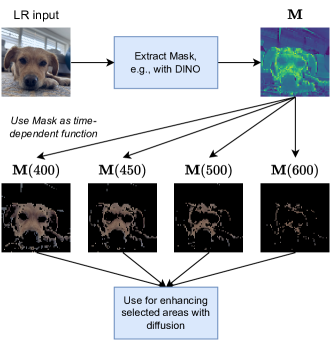
Figure 1: Time-dependent masking using $T=1000$. First, extract $\mathbf{M}$ from the LR input, e.g., with a pre-trained DINO model. Next, use values of the attention map (interval [0, 1]) and $T$ to formulate a time-dependent function. Consequently, the diffusion model can determine which pixels to refine for each time step $t$.

2.2 DINO

DINO, an acronym for DIstillation with NO labels, is a self-supervised learning approach [4]. It involves a teacher and a student network optimized to match the teacher’s output via a cross-entropy loss. Both networks share the same architecture, namely Vision Transformers (ViTs) [10].

During training, each network receives two random views of the same input image: the teacher gets global views, two $224\times 224$ crops of the original image, and the student receives local views, i.e., $96\times 96$ crops.

This setup encourages the student to learn “local-to-global” correspondences. In other words, the student network aims to predict the teacher’s output, which teaches it to infer global information from local patches. The teacher’s parameters are updated as a moving average of the student’s parameters, which helps prevent mode collapse that usually occurs when the teacher and student have identical architectures and produce congruent embeddings.

DINO’s ability to extract meaningful global features from local data is beneficial for our purpose. The self-attention maps generated by the ViTs provide insights into the image’s layout and significant regions, which we leverage to guide the diffusion process in YODA. In another context, DINO’s approach to feature extraction has also been applied to tasks like image compression [3], demonstrating its versatility and capability to capture essential image contents in its attention maps.

3 Methodology

We propose “You Only Diffuse Areas” (YODA), which optimizes the forward and backward diffusion by focusing on key regions of the image in each time step. Thus, YODA enhances overall image quality by pinpointing essential and detail-rich areas for more frequent refinement.

We begin by introducing the concept of time-dependent masking. Next, we explore how this masking can be seamlessly integrated into the training and sampling pipeline of DDPMs.

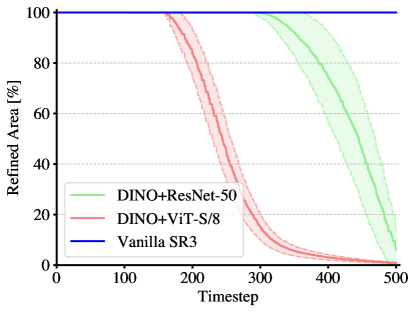
Figure 2: Refined area in percentage across time steps for the MAX combination. Note that the sampling process goes from $T=500$ to $T=0$. ResNet-50 initiates the refinement much earlier, advances more rapidly toward refining the entire image, and has a higher standard deviation.

3.1 Time-Dependent Masking

Let $\mathbf{x}$ be the input LR image, which needs to be enhanced to a SR prediction in $T$ steps. We assume an attention mask $\mathbf{M}$ of the same spatial size as $\mathbf{x}$. The attention mask $\mathbf{M}$ can be generated in various ways, and we evaluate in the experiments section different methods, in which we found that a pre-trained DINO [4] model applied to the LR image $\mathbf{x}$ generates the best attention mask. Each entry of the mask, $0\leq\mathbf{M}_{i,j}\leq 1$, reflects the importance of the corresponding spatial position in $\mathbf{x}$. For two coordinates $(i,j)$ and $(i^{\prime},j^{\prime})$ with $\mathbf{M}_{i,j}>\mathbf{M}_{i^{\prime},j^{\prime}}$, our diffusion method applies more refinement steps to the location $(i,j)$ than to $(i^{\prime},j^{\prime})$, exactly $\mathbf{M}_{i,j}-\mathbf{M}_{i^{\prime},j^{\prime}}$ more iteration steps.

Further, we advance the masking process by introducing a lower bound hyperparameter of $0<l<1$, eliminating areas that would never undergo diffusion (for $\mathbf{M}_{i,j}=0$) and ensuring a minimum number of diffusion steps in each spatial position. Specifically, we ensure that with the lower bound hyperparameter $l$, every spatial position is refined at least $l\cdot T$ times. As a result, we can formulate a time-dependent mask with the following equation:

$$\mathbf{M}(t)_{i,j}=\begin{cases}1\text{, if }T\cdot(\mathbf{M}_{i,j}+l)\geq t\\ 0\text{, otherwise}\end{cases}$$ (8)

Fig. 1 shows an example of our time-dependent masking. For each time step within the range $0\leq t\leq T$, we can logically determine whether a given spatial position $(i,j)$ should be refined. While the forward diffusion remains the same, Equation 8 necessitates a modified training and sampling procedure different from standard DDPMs.

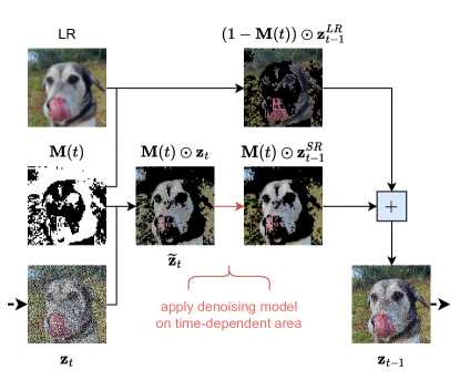
Figure 3: Our sampling process starts with masking areas that need refinement (derived from $\mathbf{z}_{t}$ and $\mathbf{M}(t)$) and LR regions, which retain the noise level needed for the next time step. Finally, the SR and LR areas are combined to form a whole image.

3.2 Optimization

We aim to confine the backward diffusion to specific areas determined by the current time step $0\leq t\leq T$ and the corresponding time-dependent mask $\mathbf{M}(t)$. This leads to a modified version of Eq. 7 as a training objective:

$$\mathcal{L}\left(\theta\right)=\mathop{\mathbb{E}}_{(\mathbf{x},\mathbf{y})}\mathop{\mathbb{E}}_{t}\bigg{\lVert}\mathbf{M}(t)\odot\left[\varepsilon_{t}-f_{\theta}\left(\mathbf{x},\mathbf{z}_{t},\gamma_{t}\right)\right]\bigg{\rVert}_{1}$$ (9)

3.3 Backward Diffusion

The backward diffusion iteratively reverses the forward diffusion, transitioning from the noisy state $\mathbf{z}_{T}$ to the clean state $\mathbf{z}_{0}$. To ensure that masked and non-masked regions are correctly connected between two successive time steps, we formulate the backward diffusion visualized in Fig. 3 similar to related inpainting methods such as RePaint [19].

At time step $t$, we identify areas that require refinement in the next time step $(t-1)$, which are derived from the output of the current iteration $\mathbf{z}_{t}$, and the current mask $\mathbf{M}(t)$:

$$\mathbf{\widetilde{z}}_{t}\leftarrow\mathbf{M}(t)\odot\mathbf{z}_{t}$$ (10)

Next, we divide the image into two components that will later form a dichotomy: $\mathbf{z}^{SR}_{t-1}$, which is the refined image in the next step, and $\mathbf{z}^{LR}_{t-1}$, the complementary LR image that remains unchanged sampled using $\mathbf{x}$ as the mean. Both components acquire the same noise level $\Sigma_{\theta}(\mathbf{\widetilde{z}}_{t},\mathbf{x},\gamma_{t})$, and can be described by:

$$\mathbf{z}^{SR}_{t-1} \sim\mathcal{N}\left(\mu_{\theta}(\mathbf{\widetilde{z}}_{t},\mathbf{x},\gamma_{t}),\Sigma_{\theta}(\mathbf{\widetilde{z}}_{t},\mathbf{x},\gamma_{t})\right)$$ (11)

$$\mathbf{z}^{LR}_{t-1} \sim\mathcal{N}\left(\mathbf{x},\Sigma_{\theta}(\mathbf{\widetilde{z}}_{t},\mathbf{x},\gamma_{t})\right)$$ (12)

The last step combines the complementing, non-overlapping areas to reconstruct a complete image:

$$\mathbf{z}_{t-1}\leftarrow\mathbf{M}(t)\odot\mathbf{z}^{SR}_{t-1}+(1-\mathbf{M}(t))\odot\mathbf{z}^{LR}_{t-1}$$ (13)

This fusion is heavily inspired by RePaint [19], where we handle unknown pixels as SR predictions that undergo diffusion while preserving known pixels as LR parts. Contrary to RePaint, we introduce a time-dependent variation. We dynamically control the spatial expansion of inpainted SR predictions over time, whereas RePaint uses the same masking in all diffusion steps. Consequently, $\mathbf{z}^{SR}_{t}$ expands as $t$ propagates to $0$, whereas $\mathbf{z}^{LR}_{t}$ shrinks in size.

S	Model	PSNR $\uparrow$	SSIM $\uparrow$	LPIPS $\downarrow$
4×	SR3	17.98	0.607	0.138
	SR3 + YODA	26.33	0.838	0.090
8×	SR3	17.44	0.631	0.147
	SR3 + YODA	25.04	0.800	0.126

Table 1: Results on face SR with 4× scaling ($64\times 64\rightarrow 256\times 256$) and 8× scaling ($64\times 64\rightarrow 512\times 512$) on CelebA-HQ. The models were trained for 1M iterations on FFHQ and a reduced batch size of 4 and 8 to fit on a single GPU, respectively.

4 Experiments

We evaluate YODA and compare its performance in tandem with SR3 for face-only, and SRDiff for general SR. We present quantitative and qualitative results for both tasks. Overall, our method achieves high-quality results for both tasks and outperforms using standard metrics such as PSNR, SSIM, and LPIPS [23].

LR

HR

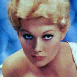
SR3
$\uparrow$ PSNR: 11.811
$\uparrow$ SSIM: ​  0.3311
$\downarrow$ LPIPS: 0.2847

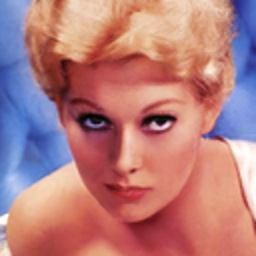
SR3+YODA
$\uparrow$ PSNR: 18.069
$\uparrow$ SSIM: ​  0.6588
$\downarrow$ LPIPS: 0.2628

Figure 4: A comparison of LR, HR, SR3, and SR3+YODA images in the $64\times 64\rightarrow 256\times 256$ setting. The color shift evident in vanilla SR3 is absent in our approach.

4.1 Training Details

The implementation is made publicly available on GitHub, which complements the official implementation of SRDiff and the unofficial implementation of SR3. All experiments were run on a single NVIDIA A100-80GB GPU.

4.1.1 Face Super-Resolution

We use the Flickr-Faces-HQ (FFHQ) dataset [14] for training, which comprises 50,000 high-quality facial images sourced from Flickr. We adopted the AdamW [18] optimizer, using a weight decay of 0.0001 and a learning rate of 5e-5. The number of sampling steps is set to $T_{train}=500$. For evaluation, we use the CelebA-HQ dataset [13], which contains 30,000 facial images. The number of sampling steps is set to $T_{eval}=200$. Furthermore, we employed 1M training iterations as in SR3 [25]. We evaluated three scenarios: $16\times 16\rightarrow 128\times 128$, $64\times 64\rightarrow 256\times 256$, and $64\times 64\rightarrow 512\times 512$. Due to the hardware requirements of SR3 and our available hardware, coupled with the absence of reported quantitative results in the original publication, our experiments with SR3 required a decrease from the originally used batch size of 256: we used a batch size of 8 for the $64\times 64\rightarrow 256\times 256$ and 4 for the $64\times 64\rightarrow 512\times 512$ scenario.

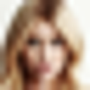
LR

HR

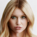
SR3
$\uparrow$ PSNR: 23.061
$\uparrow$ SSIM: ​  0.6208
$\downarrow$ LPIPS: 0.0504

SR3+YODA
$\uparrow$ PSNR: 23.289
$\uparrow$ SSIM: ​  0.6334
$\downarrow$ LPIPS: 0.0502

Figure 5: A comparison of LR, HR, SR3, and SR3+YODA images illustrates the improved quality of our proposed method for the $16\times 16\rightarrow 128\times 128$ CelebA-HQ setting.

4.1.2 General Super-Resolution

We follow the experimental design of SRDiff [15] and its hyperparameters, which are originally based on the experimental design of SRFlow [20]: For training, we employed 800 2K resolution high-quality images from DIV2K [1] and 2,650 2K images from Flickr2K [28]. For testing, we used the DIV2K validation set (100 images). Formally, $\mathbf{z}^{LR}_{t-1}$ in Eq. 13 has a mean value of 0 instead of $\mathbf{x}$ due to SRDiff’s prediction of the residual information between LR and HR.

For additional evaluation, we also tested SR3, which was originally not tested on DIV2K. For this line of experiments, we extracted $40\times 40$ sub-images with a batch size of 16, AdamW [18], a channel size of 64 with channel multipliers [1, 2, 2, 4] and $T=100$ (SRDiff’s setting).

Type	Methods	PSNR $\uparrow$	SSIM $\uparrow$	LPIPS $\downarrow$
Interpolation	Bicubic	26.70	0.77	0.409
Regression	EDSR [17]	28.98	0.83	0.270
	LIIF [5]	29.24	0.84	0.239
	RRDB [30]	29.44	0.84	0.253
GAN	RankSRGAN [32]	26.55	0.75	0.128
	ESRGAN [30]	26.22	0.75	0.124
Flow	SRFlow [20]	27.09	0.76	0.120
	HCFlow [16]	27.02	0.76	0.124
Flow + GAN	HCFlow++ [16]	26.61	0.74	0.110
VAE + AR	LAR-SR [11]	27.03	0.77	0.114
Diffusion	SR3	14.14	0.15	0.753
	SR3+YODA (ours)	27.24	0.77	0.127
	SRDiff [15]	27.41	0.79	0.136
	SRDiff + YODA (ours)	27.62	0.80	0.146

Table 2: Quantitative results of 4× general SR on the DIV2K validation set.

4.2 Results

This section provides the results of YODA. We present quantitative and qualitative results for facial and general SR using DINO to extract the dynamic attention masks for YODA. Lastly, we show our ablation study of different attention maps extracted with DINO alongside deterministic, non-DL methods to derive attention maps. We also examined aggregations of DINO attention maps.

4.2.1 Face Super-Resolution

The results are shown in Tab. 1, where an evident enhancement is observed when SR3 is coupled with YODA across all examined metrics. We explain the significant improvements by YODA with a phenomenon, which is also observed by other authors [29, 6], consistent with most SR predictions: a color shift within the SR3 predictions, which we attribute to the reduced batch size necessitated by hardware limitations. An example is shown in Fig. 4 for 8× scaling. This color shift manifested in a pronounced deviation in pixel-based metrics PSNR and SSIM but did not affect the perceptual metric LPIPS in similar significance.

YODA’s role seems to extend beyond mere performance enhancement. It actively mitigates the color shift phenomenon. This observation underscores the potential of YODA as not merely a performance enhancer but also as a stabilizing factor, particularly when faced with hardware constraints. With YODA, SR3 can be trained with a much smaller batch size and still achieves strong performance.

Fig. 5 offers another 8× scaling qualitative example between SR3 and SR3+YODA, highlighting subtle yet potentially impactful differences, especially for the pixel-based metrics PSNR and SSIM. The most notable differences can be observed around the eyes, mouth, and hair.

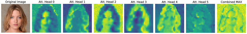
Figure 6: Comparison of attention maps derived from different DINO (ResNet-50 backbone) attention heads 0 to 5 and the combination of all attention maps (MAX). Notably, the total pixel updates of max aggregation are given the highest pixel updates in all attention heads. Blue indicates low attention values, while yellow indicates high attention values.

4.2.2 General Super-Resolution

Tab. 2 shows the 4× scaling general image SR results on the DIV2K validation set. The reported values include regression-based methods, which typically yield higher pixel-based scores (PSNR and SSIM) than generative approaches [25]. This disparity is due to PSNR/SSIM penalizing high-frequency details misaligned with the target image, a significant challenge in SR. Thus, PSNR/SSIM favors regression-based techniques for their conservative generation of high-frequency details, which minimize the risk of misalignment caused by generative hallucinations. When implemented with YODA, SRDiff demonstrates improved performance in PSNR by +0.21db and SSIM by +0.01. However, there is a minor increase in LPIPS by +0.01. Thus, our approach excels in pixel-centric metrics but sees a marginal decline in the perceptual metric.

On the other hand, we can observe a mediocre performance of SR3. Even though the hyperparameters for SR3 were not extensively studied, the integration of YODA still improves its performance notably. We address vanilla SR3’s bad performance due to low diffusion steps, low batch size, and the training on sub-images. Thus, YODA’s strengths appear more significant in SR3 than in SRDiff, as evidenced by the performance improvement. This may stem from SRDiff’s design, which focuses on diffusing within the residual image, i.e., the difference between LR and HR. Unlike SR3’s approach of using the full LR image, SRDiff’s residual image input is relatively sparse. As a result, we surmise that DINO’s attention maps might not accurately capture the essential regions of the input, possibly overvaluing areas that might not be as informative in the residual image.

Another critical distinction between SR3 and SRDiff is their incorporation of conditional information, i.e., the LR image, which we identify as a potential contributor to the reduced perceptual score. SRDiff employs an LR encoder that generates an embedding during the denoising phase. Meanwhile, SR3 directly uses the LR image during the backward diffusion. Another possible reason for the lower perceptual score could be the image size during DINO training, i.e., $224\times 224$ for the teacher network. As such, fine-tuning DINO on larger-scale images might be essential to capture more meaningful semantic features. Yet, YODA’s benefits are still instrumental as it improves pixel-based scores (PSNR and SSIM) and might unlock optimized inference latency based on sparser diffusion steps.

Model	PSNR $\uparrow$	SSIM $\uparrow$	LPIPS $\downarrow$
SR3 (reported)	23.04	0.650	n.a.
SR3 (reproduced)	22.35	0.646	0.082
Gaussian	22.13	0.602	0.260
Edge-based Seg.	22.93	0.648	0.151
SIFT	22.84	0.678	0.095
ViT-S/8 Att.-Head 0	22.91	0.650	0.105
ViT-S/8 Att.-Head 1	22.43	0.616	0.130
ViT-S/8 Att.-Head 2	22.55	0.633	0.111
ViT-S/8 Att.-Head 3	22.73	0.641	0.110
ViT-S/8 Att.-Head 4	22.85	0.645	0.097
ViT-S/8 Att.-Head 5	22.86	0.648	0.101
ViT-S/8 AVG	23.25	0.663	0.122
ViT-S/8 MAX	23.46	0.683	0.103
ResNet-50 Att.-Head 0	22.82	0.649	0.115
ResNet-50 Att.-Head 1	22.54	0.627	0.117
ResNet-50 Att.-Head 2	22.84	0.650	0.107
ResNet-50 Att.-Head 3	22.78	0.645	0.105
ResNet-50 Att.-Head 4	22.38	0.620	0.127
ResNet-50 Att.-Head 5	22.50	0.630	0.119
ResNet-50 AVG	23.55	0.682	0.093
ResNet-50 MAX	23.84	0.695	0.072

Table 3: Ablation study of SR3+YODA using different attention maps for $16\times 16\rightarrow 128\times 128$ on CelebA-HQ. The second block shows the results using non-DL importance masks, while the subsequent blocks show the performance with attention maps derived by DINO (with ViT-S/8 and ResNet-50 backbone).

4.2.3 Ablation of Attention Maps

Despite a pre-trained DINO model, we also evaluated non-deep learning-based methods to derive attention maps for guiding backward diffusion and training:

• Gaussian: Placing a simple 2D Gaussian pattern at the center of the image provides a straightforward approach, which relies on the assumption that the essential parts of an image are centered (center bias).

• Edge-based Segmentation: Using the Canny edge detector, the attention maps are defined by the edges of the image, where adjacent and near edges are connected to create defined and filled regions.

• Scale-Invariant Feature Transform (SIFT): Through Gaussian differences, SIFT provides an attention map characterized by scale invariance. It produces an attention map by applying 2D Gaussian patterns around the points of interest.

Tab. 3 presents the results of our study with several baselines and masking variants for $16\times 16\rightarrow 128\times 128$ scaling on the CelebA-HQ dataset. The evaluation of these deterministic strategies revealed mixed performance results. As expected, the straightforward Gaussian approach yielded the worst performance as it does not adapt to image features. The edge-based segmentation and SIFT methods displayed superior efficacy to the reproduced SR3 under lower batch size. However, they underperformed relative to the reported SR3 results with larger batch size [25].

In contrast, using DINO to extract attention maps improves performance for two types of CNN backbones: ResNet-50 and ViT-S/8. We tested individual attention heads (0 to 5) independently, along with combination strategies that include averaging (AVG) and selecting the maximum value (MAX). The MAX combination surfaced as a distinct method that achieved the best results compared to individual heads or the AVG combination. ResNet-50 performs best for the two backbone architectures, indicating its suitability to guide our time-dependent diffusion approach. Thus, we used the MAX aggregation of attention heads method within DINO and utilized the ResNet-50 backbone for all other experiments.

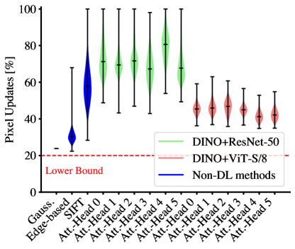
Figure 7: Ratio comparison between diffused pixels using our time-dependent masking approach and the total number of pixel updates in standard diffusion. On average, DINO with a ResNet-50 backbone leads to more pixel updates than the VIT-S/8 backbone. The lower bound $l$ is a threshold to eliminate areas that would never undergo diffusion.

Fig. 7 provides more information on the ratio of diffused pixels using our time-dependent masking and the total number of pixel updates required if diffusion was uniformly applied across all pixel locations throughout every time step (as in standard diffusion). Therefore, any result under 100% shows that not all pixels are diffused during all time steps in the sampling process. As can be seen, DINO coupled with the ResNet-50 architecture requires more total pixel updates than its implementation with ViT-S/8 or deterministic methods. Note that the ResNet-50 backbone can employ 100% of the updates for particularly exceptional scenarios, a characteristic not observed with the combination of DINO and ViT-S/8. Moreover, integrating DINO with ResNet-50 and the MAX combination demands, on average, approximately 70% of the iterative refinement steps in SR3.

The coverage can also be inspected in Fig. 6, where roughly 70% of the image is diffused according to the MAX-combined attention map. Interestingly, areas with better illumination are often weighted higher for the MAX-combined attention map. Fig. 2 illustrates areas refined over time using the MAX-combined attention maps. Here, both ResNet-50 and ViT-S/8 show similar trends in terms of refined area amounts. However, ResNet-50 initiates the refinement process much earlier (because the backward diffusion process starts from $T$ and propagates towards 0), advances more rapidly toward refining the entire image, and has a higher standard deviation, which indicates a much higher individual adaption to specific input samples.

5 Limitations & Future Work

A notable constraint of this study is its dependence on a pre-trained DINO model, thereby inheriting its limitations. For instance, to effectively handle medical image SR, DINO would require fine-tuning tailored to the characteristics of medical imagery. Additionally, DINO is explicitly trained for resolutions such as $224\times 224$, which may not suffice for image SR applications with much higher spatial sizes. An ideal solution would be a scale-invariant extraction of attention maps. Another limitation is that YODA introduces a new hyperparameter: the lower bound, which represents the minimum number of diffusion steps that must be defined before training and should be analyzed in more detail in future work. Also, we linearly correspond the attention mask values to the importance of each pixel, which is not necessarily the best relationship and demands further investigation. For further research, explorations of unconditional image generation with YODA, such as text-to-image translation, and developing other innovative techniques to extract attention maps could be exciting avenues. Moreover, it would be interesting to see YODA perform related image restoration tasks, such as deblurring or unsupervised SR.

6 Conclusion

In this work, we presented a novel ”You Only Diffuse Areas” (YODA) approach for attention-guided diffusion-based image SR that emphasizes specific areas through time-dependent masking. With a pre-trained DINO model, we can generate attention maps that reflect the pixel-wise importance of each scene. As a result, we were able to guide the diffusion process by focusing on key regions in each time step while providing a fusion technique to ensure that masked and non-masked image regions are correctly connected between two successive time steps. This targeting allows for a more efficient transition to high-resolution outputs, prioritizing areas that gain the most from iterative refinements, such as detail-intensive objects.

First, we examined different techniques to derive attention maps, including deterministic methods and the self-supervised method DINO. Our investigation on the $16\times 16\rightarrow 128\times 128$ face SR case led to selecting DINO with a MAX combination of attention maps as the optimal strategy, which we adopted for the following experiments. Our subsequent evaluations compared YODA against vanilla SR3 in face SR tasks ($64\times 64\rightarrow 256\times 256$ and $64\times 64\rightarrow 512\times 512$) and against vanilla SRDiff in general SR with 4x scaling. In both tasks, YODA outperformed the state-of-the-art diffusion-based techniques by extending them with YODA (plug&play), showcasing superiority in core metrics, including PSNR, SSIM, and LPIPS.

Beyond performance enhancement, YODA stabilizes training. It mitigates the color shift phenomenon that emerges when a reduced batch size constrains vanilla SR3 due to hardware limitations. As a result, YODA consistently delivers impressive quality using smaller batch sizes than standard SR3. Therefore, SR3 combined with YODA can be used on more commonly available and possibly less expensive hardware, enhancing accessibility.

References

- [1] Eirikur Agustsson and Radu Timofte. Ntire 2017 challenge on single image super-resolution: Dataset and study. In Proceedings of the IEEE conference on computer vision and pattern recognition workshops, pages 126–135, 2017.
- [2] Saeed Anwar and Nick Barnes. Densely residual laplacian super-resolution. IEEE Transactions on Pattern Analysis and Machine Intelligence, 2020.
- [3] Federico Baldassarre, Alaaeldin El-Nouby, and Hervé Jégou. Variable rate allocation for vector-quantized autoencoders. In ICASSP 2023-2023 IEEE International Conference on Acoustics, Speech and Signal Processing (ICASSP), pages 1–5. IEEE, 2023.
- [4] Mathilde Caron, Hugo Touvron, Ishan Misra, Hervé Jégou, Julien Mairal, Piotr Bojanowski, and Armand Joulin. Emerging properties in self-supervised vision transformers. In Proceedings of the IEEE/CVF international conference on computer vision, pages 9650–9660, 2021.
- [5] Yinbo Chen, Sifei Liu, and Xiaolong Wang. Learning continuous image representation with local implicit image function. In Proceedings of the IEEE/CVF conference on computer vision and pattern recognition, pages 8628–8638, 2021.
- [6] Jooyoung Choi, Jungbeom Lee, Chaehun Shin, Sungwon Kim, H Kim, and S Yoon. Perception prioritized training of diffusion models. 2022 ieee. In CVF Conference on Computer Vision and Pattern Recognition (CVPR), pages 11462–11471, 2022.
- [7] Hyungjin Chung, Eun Sun Lee, and Jong Chul Ye. Mr image denoising and super-resolution using regularized reverse diffusion. IEEE Transactions on Medical Imaging, 2022.
- [8] Hyungjin Chung, Byeongsu Sim, and Jong Chul Ye. Come-closer-diffuse-faster: Accelerating conditional diffusion models for inverse problems through stochastic contraction. In Proceedings of the IEEE/CVF Conference on Computer Vision and Pattern Recognition, pages 12413–12422, 2022.
- [9] Chao Dong, Chen Change Loy, Kaiming He, and Xiaoou Tang. Image super-resolution using deep convolutional networks. IEEE transactions on pattern analysis and machine intelligence, 38(2):295–307, 2015.
- [10] Alexey Dosovitskiy, Lucas Beyer, Alexander Kolesnikov, Dirk Weissenborn, Xiaohua Zhai, Thomas Unterthiner, Mostafa Dehghani, Matthias Minderer, Georg Heigold, Sylvain Gelly, et al. An image is worth 16x16 words: Transformers for image recognition at scale. arXiv preprint arXiv:2010.11929, 2020.
- [11] Baisong Guo, Xiaoyun Zhang, Haoning Wu, Yu Wang, Ya Zhang, and Yan-Feng Wang. Lar-sr: A local autoregressive model for image super-resolution. In Proceedings of the IEEE/CVF Conference on Computer Vision and Pattern Recognition, pages 1909–1918, 2022.
- [12] Jonathan Ho, Ajay Jain, and Pieter Abbeel. Denoising diffusion probabilistic models. Advances in Neural Information Processing Systems, 33:6840–6851, 2020.
- [13] Tero Karras, Timo Aila, Samuli Laine, and Jaakko Lehtinen. Progressive growing of gans for improved quality, stability, and variation. arXiv preprint arXiv:1710.10196, 2017.
- [14] Tero Karras, Samuli Laine, and Timo Aila. A style-based generator architecture for generative adversarial networks. In Proceedings of the IEEE/CVF conference on computer vision and pattern recognition, pages 4401–4410, 2019.
- [15] Haoying Li, Yifan Yang, Meng Chang, Shiqi Chen, Huajun Feng, Zhihai Xu, Qi Li, and Yueting Chen. Srdiff: Single image super-resolution with diffusion probabilistic models. Neurocomputing, 479:47–59, 2022.
- [16] Jingyun Liang, Andreas Lugmayr, Kai Zhang, Martin Danelljan, Luc Van Gool, and Radu Timofte. Hierarchical conditional flow: A unified framework for image super-resolution and image rescaling. In Proceedings of the IEEE/CVF International Conference on Computer Vision, pages 4076–4085, 2021.
- [17] Bee Lim, Sanghyun Son, Heewon Kim, Seungjun Nah, and Kyoung Mu Lee. Enhanced deep residual networks for single image super-resolution. In Proceedings of the IEEE conference on computer vision and pattern recognition workshops, pages 136–144, 2017.
- [18] Ilya Loshchilov and Frank Hutter. Decoupled weight decay regularization. arXiv preprint arXiv:1711.05101, 2017.
- [19] Andreas Lugmayr, Martin Danelljan, Andres Romero, Fisher Yu, Radu Timofte, and Luc Van Gool. Repaint: Inpainting using denoising diffusion probabilistic models. In Proceedings of the IEEE/CVF Conference on Computer Vision and Pattern Recognition, pages 11461–11471, 2022.
- [20] Andreas Lugmayr, Martin Danelljan, Luc Van Gool, and Radu Timofte. Srflow: Learning the super-resolution space with normalizing flow. In Computer Vision–ECCV 2020: 16th European Conference, Glasgow, UK, August 23–28, 2020, Proceedings, Part V 16, pages 715–732. Springer, 2020.
- [21] Brian B. Moser, Stanislav Frolov, Federico Raue, Sebastian Palacio, and Andreas Dengel. Dwa: Differential wavelet amplifier for image super-resolution. In Lazaros Iliadis, Antonios Papaleonidas, Plamen Angelov, and Chrisina Jayne, editors, Artificial Neural Networks and Machine Learning – ICANN 2023, pages 232–243, Cham, 2023. Springer Nature Switzerland.
- [22] Brian B Moser, Stanislav Frolov, Federico Raue, Sebastian Palacio, and Andreas Dengel. Waving goodbye to low-res: A diffusion-wavelet approach for image super-resolution. CoRR, abs/2304.01994, 2023.
- [23] Brian B. Moser, Federico Raue, Stanislav Frolov, Sebastian Palacio, Jörn Hees, and Andreas Dengel. Hitchhiker’s guide to super-resolution: Introduction and recent advances. IEEE Transactions on Pattern Analysis and Machine Intelligence, pages 1–21, 2023.
- [24] Robin Rombach, Andreas Blattmann, Dominik Lorenz, Patrick Esser, and Björn Ommer. High-resolution image synthesis with latent diffusion models. In Proceedings of the IEEE/CVF conference on computer vision and pattern recognition, pages 10684–10695, 2022.
- [25] Chitwan Saharia, Jonathan Ho, William Chan, Tim Salimans, David J Fleet, and Mohammad Norouzi. Image super-resolution via iterative refinement. IEEE Transactions on Pattern Analysis and Machine Intelligence, 2022.
- [26] Jascha Sohl-Dickstein, Eric Weiss, Niru Maheswaranathan, and Surya Ganguli. Deep unsupervised learning using nonequilibrium thermodynamics. In International Conference on Machine Learning, pages 2256–2265. PMLR, 2015.
- [27] Wanjie Sun and Zhenzhong Chen. Learned image downscaling for upscaling using content adaptive resampler. IEEE Transactions on Image Processing, 29:4027–4040, 2020.
- [28] Radu Timofte, Shuhang Gu, Jiqing Wu, and Luc Van Gool. Ntire 2018 challenge on single image super-resolution: Methods and results. In Proceedings of the IEEE conference on computer vision and pattern recognition workshops, pages 852–863, 2018.
- [29] Jianyi Wang, Zongsheng Yue, Shangchen Zhou, Kelvin CK Chan, and Chen Change Loy. Exploiting diffusion prior for real-world image super-resolution. arXiv preprint arXiv:2305.07015, 2023.
- [30] Xintao Wang, Ke Yu, Shixiang Wu, Jinjin Gu, Yihao Liu, Chao Dong, Yu Qiao, and Chen Change Loy. Esrgan: Enhanced super-resolution generative adversarial networks. In Proceedings of the European conference on computer vision (ECCV) workshops, pages 0–0, 2018.
- [31] Jay Whang, Mauricio Delbracio, Hossein Talebi, Chitwan Saharia, Alexandros G Dimakis, and Peyman Milanfar. Deblurring via stochastic refinement. In Proceedings of the IEEE/CVF Conference on Computer Vision and Pattern Recognition, pages 16293–16303, 2022.
- [32] Wenlong Zhang, Yihao Liu, Chao Dong, and Yu Qiao. Ranksrgan: Generative adversarial networks with ranker for image super-resolution. In Proceedings of the IEEE/CVF International Conference on Computer Vision, pages 3096–3105, 2019.
- [33] Kai Zhao, Alex Ling Yu Hung, Kaifeng Pang, Haoxin Zheng, and Kyunghyun Sung. Partdiff: Image super-resolution with partial diffusion models. arXiv preprint arXiv:2307.11926, 2023.