1 Introduction

Light mediators – new massive, unstable particles that couple to the SM – have seen tremendous interest over the past decade (for reviews, see [1, 2]). They are essential to models of light dark matter [3, 4, 5], providing mechanisms that lead to the correct abundance as well as providing detectable signals in the myriad landscape of light dark matter detection experiments. A panoply of experiments have been considered to gain sensitivity to these mediators.

Specializing to light $U(1)$ vector boson mediators, several varieties have been considered: the dark photon (for a recent review, see [6]); $U(1)_{B-L}$ (early discussions include [7, 8, 9] and a review of massive $Z^{\prime}$s [10]), while gauged $U(1)_{B-L}$ as a light mediator has been considered in detail in [11, 12, 13, 14]; $U(1)_{B}$ [15, 16, 17]; and flavor-dependent $U(1)$s such as $U(1)_{\mu-\tau}$ [18, 19, 20] (some recent work [21, 22]). A huge variety of constraints restrict the parameter space of these light vector bosons [11, 12, 13, 14] including colliders, fixed target experiments, energy loss from stars; energy loss from supernovae, changes to big-bang nucleosynthesis; etc.

Our focus in this paper is to calculate the contributions to the effective number of relativistic species, $N_{\rm eff}$, from a light $U(1)_{B-L}$ gauge boson mediator $X$, determining both the existing constraints and prospects for future CMB observatories. Precision determination of $N_{\text{eff}}$, from CMB power spectra [23, 24] and primordial element abundances [25, 26, 27, 28] is in strong agreement with SM prediction [29, 30, 31, 32, 33, 34, 35, 36, 37, 38, 39, 40]. This makes $N_{\text{eff}}$ a powerful tool in testing BSM physics that affects early universe cosmology before recombination [41, 42, 43, 44, 45, 46, 47, 48, 49, 50, 51, 52, 53, 54, 21, 55, 56, 57, 58]. We carry out the full Boltzmann evolution, allowing the $X$ boson to “freeze in” [59], become nonrelativistic, redshift as matter, and then decay back into SM states, modifying $\Delta N_{\rm eff}$. Earlier calculations have considered the contributions to $\Delta N_{\rm eff}$ from the freeze in of a dark photon [55] and $U(1)_{\mu-\tau}$ [21]. The cosmological constraints from $\Delta N_{\rm eff}$ on the dark photon are relatively strong when the dark photon mass is near the temperature of BBN, $\sim 1$ MeV, when the dark photon can interact with the electron plasma and thus (indirectly) affect the neutrino energy density, but weaker below this since the dark photon does not interact with neutrinos. By contrast, mediators that freeze in from their interactions with neutrinos have substantially stronger constraints, e.g., $U(1)_{\mu-\tau}$ [21]. In this paper, we utilize the formalism and approximations outlined in [54, 21, 56], extended and applied to the case of a $U(1)_{B-L}$ gauge boson.

The central observation is that an out-of-equilibrium abundance of new particles that interact with the SM can be well approximated by using equilibrium distributions with nonzero chemical potentials. We will discuss the formalism and approximations in detail, as applied to $U(1)_{B-L}$. The result is that since $U(1)_{B-L}$ has a nonzero coupling to neutrinos, there are strong bounds from $\Delta N_{\rm eff}$ from the CMB that get stronger with decreasing mass of $X$, down to of order $m_{X}\sim 1$ eV. In the regime $m_{X}<2m_{e}$, our results are qualitatively consistent with a similar analysis done for $U(1)_{\mu-\tau}$ [21]. At even smaller masses, $m_{X}\lesssim 1$ eV, fifth force constraints [60, 61, 62, 63] become very strong and dominate the bounds [11]. For gauge boson masses near (and below) $1$ eV, a more sophisticated treatment of the CMB is necessary to fully elucidate cosmological bounds. We will comment on this in the Discussion.

To our knowledge, the first paper that considered constraints on the mass and coupling of a light $U(1)_{B-L}$ gauge boson from its effects on $\Delta N_{\rm eff}$ is [64]. They considered a light $U(1)_{B-L}$ gauge boson with just left-handed neutrinos among the fermionic relativistic degrees of freedom. The critical difference between our study and [64] is that the latter only considered the constraints from $\Delta N_{\rm eff}$ from BBN, using simple thermalization scaling arguments. Ref. [64] found that for $m_{X}\gtrsim 10$ MeV, requiring the scattering process $e^{-}\nu\rightarrow e^{-}\nu$ through off-shell $X$ exchange is not larger than the weak interaction sets a constraint. We verify this constraint also applies to $\Delta N_{\rm eff}$ measured by the CMB, using our Boltzmann equation evolution. Ref. [64] also considered $m_{X}<10$ MeV. In this region, [64] required only that $X\leftrightarrow\nu\bar{\nu}$ did not reach thermal equilibrium at $T\sim 1$ MeV, so that $X$ does not contribute excessively to $\Delta N_{\rm eff}$ during BBN. As we will see, we find much stronger constraints in the region $m_{X}<10$ MeV from detailed numerical calculations of $\Delta N_{\rm eff}$ at the CMB era as well as strong constraints on the helium mass fraction $Y_{p}$, at the BBN era.

There are also constraints on very weakly coupled mediators that are completely out-of-equilibrium, but decay on timescales that can disrupt BBN or to cause spectral distortion in the CMB [49, 65, 57]. We show these constraints on the parameter space of $U(1)_{B-L}$, obtained from [57], that are complementary to our results.

2 Gauged U(1)_B-L: Majorana and Dirac Neutrino Cases

$U(1)_{B-L}$ is among the most interesting possible new forces since it is the only flavor-universal global symmetry of the SM that is gaugeable. All mixed $U(1)_{B-L}\times{\rm SM}^{2}$ anomalies automatically vanish within the SM. The $[U(1)_{B-L}]^{3}$ anomaly remains, requiring additional chiral fermions that transform under just $U(1)_{B-L}$. The simplest solution is to add one chiral fermion per generation with lepton number equal and opposite to $\nu_{L}$, namely, one right-handed neutrino per generation.

To establish notation, gauged $U(1)_{B-L}$ is mediated by a vector boson $X^{\mu}$ that interacts with the SM quarks and leptons with charge

$$q_{f}=(B-L)_{f}=\left\{\begin{array}[]{lcl}+1/3&&Q_{L},\;u_{R},\;d_{R}\\ -1&&L,\;e_{R},\;\nu_{R}\end{array}\right.\,,$$ (1)

where we have written the fermions in four-component notation consistent with [66]. We assume $U(1)_{B-L}$ is broken, and so $X$ acquires a mass $m_{X}$. The spontaneous breaking of $U(1)_{B-L}$ can be accomplished by introducing a complex scalar, $\phi_{X}$, transforming under $B-L$ with charge $q_{X}$, and gauge coupling $g_{X}$, with a potential engineered to spontaneously break the symmetry. The scalar Lagrangian is

$$\mathcal{L}\;=\;(D_{\mu}\phi_{X})^{\dagger}D^{\mu}\phi_{X}-V(\phi_{X})$$ (2)

where $D^{\mu}\equiv\partial^{\mu}-ig_{X}q_{X}X^{\mu}$, with

$$V(\phi_{X})\;=\;\lambda_{X}\left(\phi_{X}^{\dagger}\phi_{X}-\frac{v_{X}^{2}}{2}\right)^{2}$$ (3)

and the minimum of the scalar potential occurs at $\langle\phi_{X}\rangle=v_{X}/\sqrt{2}$. Expanding around the minimum, with $\phi_{X}=(h_{X}+v_{X})/\sqrt{2}$, where $h_{X}$ is the $B-L$ Higgs boson, the physical states in the theory have masses

$$X^{\mu}: m_{X}\,=\,g_{X}q_{X}v_{X}$$ (4)

$$h_{X}: m_{h_{X}}^{2}\,=\,2\lambda_{X}v_{X}^{2}\;.$$ (5)

Throughout the paper, we work in the limit $g_{X}q_{X}\ll\lambda_{X}$, and so, $m_{X}\ll m_{h_{X}}$. Consequently, we will not need to consider the $h_{X}$ participating in the degrees of freedom in the thermal bath for $\Delta N_{\rm eff}$ calculations. The ability to adjust the $B-L$ charge of $\phi_{X}$ implies $m_{X}$ can be made arbitrarily small relative to $g_{X}v_{X}$. That is, from the perspective of the gauge and Higgs sector, one can independently adjust $m_{X}$ and $g_{X}$ (as well as $m_{h_{X}}$, through $\lambda_{X}$).

2.1 Neutrino masses: Majorana and Dirac Cases

We do need to address neutrino masses. Given that $U(1)_{B-L}$ is gauged, the usual dimension-5 Weinberg operator for Majorana neutrino masses, $(LH)^{2}/\Lambda$, is forbidden. Instead, Yukawa couplings of left-handed and right-handed neutrinos are permitted,

$$y_{D}^{ij}\bar{L}_{i}H^{\dagger}\nu_{R,j}+h.c.\,,$$ (6)

giving neutrinos Dirac masses that preserve $U(1)_{B-L}$. This “Dirac case” is one of the two cases we will consider in this paper. In the Dirac case, since neutrinos acquire their mass from Yukawa couplings to the SM Higgs field, there is (still) no restriction on the ability to adjust $m_{X}$ and $g_{X}$ independently.

The alternative, “Majorana case”, is one where the right-handed neutrinos that are required to cancel the $[U(1)_{B-L}]^{3}$ anomaly acquire Majorana masses after $U(1)_{B-L}$ is spontaneously broken. When combined with the Dirac mass terms, Eq. (6), after electroweak symmetry is broken, this leads to the usual see-saw formula that results in left-handed neutrinos acquiring small Majorana masses. Right-handed neutrinos can acquire mass with just one Higgs field transforming under $U(1)_{B-L}$ if the $B-L$ charge is fixed to be $q_{X}=\pm 2$, such that Yukawa-like interactions are permitted,

$$\frac{y_{M}^{ij}}{2}\nu_{R,i}^{c}\nu_{R,j}^{c}\phi_{X}^{(\dagger)}+h.c.\,,$$ (7)

where $\nu_{R,i}^{c}$ are the right-handed neutrinos written with 2-component left-handed fermion notation (in order to avoid Majorana notation). In this scenario, the vev of $\phi_{X}$ not only gives mass to the gauge boson, but it also gives Majorana masses to the right-handed neutrinos, $M_{R}\sim y_{M}v_{X}$.

For us, the key distinction is that in the Majorana case, the right-handed neutrinos can be much heavier, and thus not contribute in any way to $\Delta N_{\rm eff}$. This is in contrast to the Dirac scenario, where if the right-handed neutrinos were ever in equilibrium (through, for example, $X^{\mu}$ exchange), they necessarily contribute to $\Delta N_{\rm eff}$ [67]. The size of the contribution to $\Delta N_{\rm eff}$ is controlled just by the dilution of the number of relativistic degrees of freedom after heavier SM fields annihilate (or decay) and dump their entropy into the photon bath.

It is interesting to consider the bounds on the Majorana masses for right-handed neutrinos from cosmology. Obviously if the right-handed neutrinos were in thermal equilibrium with the SM, they would excessively contribute to $\Delta N_{\rm eff}$ during BBN and CMB if their mass were less than approximately $10$ MeV. Thermal equilibrium is naturally achieved through $X^{\mu}$ exchange, so long as $g_{X}$ is not excessively small. (We’ll quantify this in detail later in the paper.) Once the right-handed neutrinos are heavier than about $10$ MeV, their abundance would be at least somewhat suppressed as they become nonrelativistic once the temperature of the Universe drops well below their mass.

Even if right-handed neutrinos decoupled early in the Universe, they can and will decay to left-handed neutrinos and a (possibly off-shell) Higgs boson, with a significant suppression in the rate due to the smallness of the (Dirac) Yukawa coupling of the right-handed neutrinos to the left-handed neutrinos. In Appendix A, we estimate the rate, and find that for $M_{R}\gtrsim 20$ GeV, the right-handed neutrinos decay before the onset of BBN.

Finally, it is also instructive to consider the case where $U(1)_{B-L}$ is explicitly broken without any scalar sector, i.e., a Stückelberg mass for the $X$ vector field (for a recent detailed discussion of the Stückelberg mechanism, see [68]). In the Dirac scenario, we can stop there, since Dirac masses respect $U(1)_{B-L}$ (see also [12]). (This is equivalent, in the spontaneously broken theory, to holding $m_{X}=q_{X}g_{X}v_{X}$ fixed, $\lambda_{X}$ fixed, but then taking $q_{X}\ll 1$ while $v_{X}$ is taken large. This limit permits any (perturbative) value for $g_{X}$.) In the Majorana case, we must also explicitly break $U(1)_{B-L}$ by $2$ units when writing explicit Majorana masses $(M_{R})_{ij}\nu^{c}_{i}\nu^{c}_{j}+h.c.$. The explicit breaking implies the $[U(1)_{B-L}]^{3}$ anomaly will appear below the scale $M_{R}$. Thus, the right-handed neutrinos induce a 3-loop anomalous contribution to the mass of the (Stückelberg) $X^{\mu}$ vector field. The size of this contribution is easily estimated [69, 70]

$$\Delta m_{X}\simeq\frac{g_{X}^{3}M_{R}}{64\pi^{3}}$$ (8)

which implies a lower bound on the mass of $X^{\mu}$ that decreases rapidly as $g_{X}$ is lowered. This bound is always weaker than Eq. (46), so that if we require right-handed neutrinos decay before BBN, there is no further constraint. Only if $M_{R}$ were large, such as a traditional see-saw mechanism with $y_{D}\sim 1$, with $M_{R}\sim 10^{14-15}$ GeV, would there be any constraint at all on $g_{X}$, though even then this constraint is quite mild.

3 Effective Number of Relativistic Species: $N_{\text{eff}}$

In standard cosmology at temperature $T\sim 10$ MeV [71], electrons, photons, and neutrinos were in thermal equilibrium. As the universe cooled, the weak interaction rate dropped below the Hubble expansion rate and neutrinos decoupled from the electromagnetic plasma around $T\sim 2$ MeV. As the universe continued to cool, the temperature dropped below the electron mass, $e^{+}e^{-}$ annihilation depleted the vast majority of charged leptons. In the limit of instantaneous neutrino decoupling, the electron-positron entropy was transferred solely to photons resulting in a temperature ratio of $T_{\gamma}/T_{\nu}=(11/4)^{1/3}\approx 1.401$ after annihilation completed. However, the weak interaction remained slightly active during $e^{+}e^{-}$ annihilation, resulting in a small but appreciable heating of neutrinos. This gives rise to a small increase to the energy density of neutrinos, conventionally defined by the effective number of relativistic species,

$$N_{\text{eff}}\;=\;\frac{8}{7}\left(\frac{11}{4}\right)^{4/3}\left(\frac{\rho_{\text{rad}}-\rho_{\gamma}}{\rho_{\gamma}}\right),$$ (9)

which is the ratio of non-photon to photon radiation density. Any new BSM radiation density present well before recombination can be treated as an additional contribution to $N_{\text{eff}}$. The normalization in Eq. (9) is chosen such that $N_{\text{eff}}=N_{\nu}=3$ in the instantaneous neutrino decoupling limit.

The state-of-the-art calculation in the SM gives $N_{\text{eff}}^{\text{SM}}=3.045$-$3.046$, that takes into higher order corrections, non-thermal neutrino distribution functions, neutrino oscillations, etc. [30, 29]. In this paper, we have followed Refs. [54, 56] that have provided an efficient calculation of $N_{\rm eff}$ which employs certain approximations that nevertheless result in excellent accuracy, which we will discuss in detail in Sec. 4.1. For instance, using this method, we obtain the photon-to-neutrino temperature ratio, the neutrino chemical potential, and $N_{\rm eff}$ in the SM

$$T_{\gamma}/T_{\nu}=1.3945\,,\quad\quad\quad\mu_{\nu}/T_{\nu}=-4.82\times 10^{-3}\,,\quad\quad N_{\text{eff}}^{\text{SM}}=3.042\,.$$ (10)

The point of re-doing the SM calculation here is to demonstrate that we can achieve reasonable accuracy of $N_{\rm eff}$ even with the approximations that have been employed. The very small $\sim 0.1\%$ discrepancy between our calculation and the precise determination is slightly accidental – some of the effects we have neglected, that contribute at a level of $\sim 0.3\%$, happen to very nearly cancel out when summed together (see [56] for details). In any case, our calculation is able to reproduce the non-instantaneous decoupling of neutrinos in the SM to an accuracy of order $\Delta N_{\rm eff}\sim 0.01$.

After $e^{+}e^{-}$ annihilation is complete, the number of relativistic degrees of freedom remains the same in the SM down to the CMB era. In the presence of physics beyond the SM, there can be new degrees of freedom that appear (or disappear) before or after BBN. This can be characterized by the number of relativistic degrees of freedom at CMB, $N_{\rm eff}^{\rm CMB}$, to be distinguished from the number of relativistic degrees of freedom at BBN, $N_{\rm eff}^{\rm BBN}$. In this paper, $N_{\text{eff}}$ refers exclusively to $N_{\rm eff}^{\rm CMB}$, and hereafter $N_{\text{eff}}$ and $\Delta N_{\text{eff}}$ refer to the quantities at the CMB era. We do, however, calculate the shift to the helium mass fraction $Y_{p}$ at BBN, separately from $\Delta N_{\text{eff}}$. We will present our calculations of $N_{\text{eff}}$ in Sec. 5 and $Y_{p}$ in Sec. 7, and compare to the observational determinations at the end of each of those sections.

4 Early Universe Thermodynamics

Our method to calculate thermodynamic quantities in the early universe utilizes several approximations in order to solve the Boltzmann equations that were described in detail in [54, 56]. The key insight from [54, 56] is that we can approximate the effects of out-of-equilibrium (“freeze-in”) $X$ bosons using equilibrium distributions with nonzero chemical potentials. How this works requires some explanation. At temperatures near BBN, the dominant contributions to the energy density are from electrons (and positions), photons, and neutrinos. In the SM, the annihilation and scattering rates between electrons, positions, and photons is very efficient ensuring $T_{\gamma}=T_{e}$. Since photon number is not conserved, the processes $e^{+}e^{-}\leftrightarrow\gamma$, $e^{+}e^{-}\leftrightarrow\gamma\gamma$, and $e^{+}e^{-}\leftrightarrow\gamma\gamma\gamma$ imply that the chemical potential for photons, electrons and positions vanishes, $\mu_{\gamma}=\mu_{e}=0$ (to a very good approximation [72]). When neutrino-electron scattering is active for temperatures $T\gtrsim 2$ MeV, the processes $e^{+}e^{-}\leftrightarrow\bar{\nu}_{\alpha}\nu_{\alpha}$, $e^{\pm}\nu_{\alpha}\leftrightarrow e^{\pm}\nu_{\alpha}$, and $e^{\pm}\bar{\nu}_{\alpha}\leftrightarrow e^{\pm}\bar{\nu}_{\alpha}$ ensure that $\mu_{\nu}\simeq 0$. Hence, in the SM, chemical potentials do not play a critical role in determining the thermodynamic evolution near and below the BBN era.

When we introduce a light $U(1)_{B-L}$ gauge boson $X$, there are three possible regimes of interest: heavy ($m_{X}\gg 1$ MeV), intermediate ($m_{X}\sim 1$ MeV), and light ($m_{X}\ll 1$ MeV). In all regimes, we assume $\mu_{\gamma}=\mu_{e}=0$ throughout the Boltzmann evolution, given that the electromagnetic interactions will always be much faster than interactions among $X$ bosons. Nevertheless, we allow for chemical potentials for $X$ and neutrinos to develop and evolve with temperature, as $X$ freezes-in through its very weak interactions with the SM. As we will see, the thermodynamic evolution of the SM particles plus $X$ will be quite different in these different regimes.

In the heavy regime, $m_{X}\gg 1$ MeV, as the temperature drops below $m_{X}$, the $X$ bosons become nonrelativistic while the weak interactions that keep electrons and neutrinos in thermal and chemical equilibrium remain active. At these high temperatures, there is competition between $1\leftrightarrow 2$ processes involving $X\leftrightarrow\nu\bar{\nu}$, that will cause $\mu_{X}$ and $\mu_{\nu}$ to develop, and the electroweak-mediated $2\leftrightarrow 2$ processes, that drive $\mu_{\nu}\rightarrow 0$. Initially, $X$ is out-of-equilibrium, and so a chemical potential for $X$ and neutrinos can (and will) develop. As the temperatures decrease, $X$ becomes nonrelativistic, the $2\leftrightarrow 2$ processes dominate, driving $\mu_{\nu}$ (and $\mu_{X}$) to small values. At still larger masses, for temperatures $10\;{\rm MeV}\lesssim T\ll m_{X}$, the $1\leftrightarrow 2$ processes are irrelevant, and instead off-shell $X$-exchange can contribute to $2\leftrightarrow 2$ processes qualitatively similar to electroweak gauge boson exchange. Here, there is a constraint on the strength of the $X$ boson interactions with the SM that arises from delaying neutrino freeze-out, but this is much weaker than the constraints from lighter masses, as we will see below.

In the light regime, when $m_{X}\ll 1$ MeV, electron-position annihilation is fully complete, leaving only photons, neutrinos, and $X$ as the relativistic degrees of freedom. In this regime, neutrinos are out of thermal and chemical equilibrium with the SM, and thus as $X$ freezes-in, the evolution of Boltzmann equations result in a chemical potential for $X$ and neutrinos through the process is $X\leftrightarrow\nu\bar{\nu}$. If this is efficient enough to reach chemical equilibrium, $\mu_{X}=2\mu_{\nu}$. Note that since $U(1)_{\rm B-L}$ is flavor-conserving, we necessarily have $\mu_{\nu}=\mu_{\bar{\nu}}$.

Finally, the intermediate regime, $m_{X}\sim 1$ MeV, is the trickiest one to model. When $T\sim 1$ MeV, the weak interactions have recently decoupled, and so the $2\leftrightarrow 2$ electroweak processes that enforce $\mu_{\nu}\simeq 0$ have just recently shut off. This means that as a chemical potential for $\mu_{X}$ develops from its out-of-equilibrium production, the resulting $\mu_{\nu}$ that also develops, can remain. However, electron-photon interactions are in thermal and chemical equilibrium, and so $\mu_{e}=0$. If $X$ were to be in thermal equilibrium with both electrons and neutrinos, the electron interactions $X\leftrightarrow e^{+}e^{-}$ would bias $\mu_{X}\simeq 0$. Instead, when $X$ is out-of-equilibrium, a chemical potential for $X$ can develop as $X$ freezes-in from both $e^{+}e^{-}\rightarrow X$ and $\nu\bar{\nu}\rightarrow X$ interactions. As the universe cools, more $X$ is produced, but then $e^{+}e^{-}$ annihilation into photons rapidly depletes the electron-positron bath. This means $X$ could reach thermal equilibrium with neutrinos, with a nonzero chemical potential, since the remaining electrons and positions have dropped out of chemical equilibrium.

4.1 Approximations

We assume that all fermions and bosons follow Fermi-Dirac (FD, positive) and Bose-Einstein (BE, negative), $f(E)=[e^{(E-\mu)/T}\pm 1]^{-1}$ distribution functions respectively. This assumption is well-established when the energy and momentum exchange between particles is efficient. If interactions are not fully efficient, i.e. out-of-equilibrium evolution, distributions may obtain spectral distortion corrections. An example of this is shown in Figures $9,10$ of [21] for the case of $U(1)_{L_{\mu}-L_{\tau}}$. These corrections are expected to be small.

We assume, to an excellent approximation, that the electron/positron plasma is highly thermalized with the photon plasma such that $T_{\gamma}=T_{e}$ and $\mu_{\gamma}=\mu_{e}=0$. Here, we leverage the strong annihilation and scattering rate between electrons, positrons, and photons and that the number of photons is not conserved in the early universe. As for neutrinos, we describe a neutrino fluid with a single distribution characterized by $T_{\nu}\equiv T_{\nu_{e}}=T_{\nu_{\mu}}=T_{\nu_{\tau}}$ and $\mu_{\nu}$. Here, we ignored neutrino oscillations which become active for temperatures $T=3$-$5$ MeV, [73, 74], and model this effect by setting the temperature of the different neutrino species equal. The correction due to neutrino oscillations in SM is $\Delta N_{\text{eff}}=0.0007$ [29]. The correction due to evolving distinct neutrino species temperature rather than a single $T_{\nu}$ was found to be $\Delta N_{\text{eff}}=0.001$ using the approximations [54, 56] we employ in this paper.

Finally, for the collision terms we have implemented the correct particle distributions for the $1\leftrightarrow 2$ collision terms, and approximate particle distributions for $2\leftrightarrow 2$ collision terms. For the $1\leftrightarrow 2$ processes, this means we use a Fermi-Dirac distribution for fermions, a Bose-Einstein distribution for bosons, and include Pauli blocking and Bose enhancement. For the $2\leftrightarrow 2$ processes, we use Maxwell-Boltzmann distributions for all particles, which reduces the number of integrations needed for the collision terms and significantly decreases the numerical computation time. Our implementation of using the correct statistics for the $1\leftrightarrow 2$ collision processes is motivated by the relative importance of these processes in determining an accurate calculation of $N_{\text{eff}}$. While the qualitative features of our results remain unaffected even if Maxwell-Boltzmann distributions were used for $1\leftrightarrow 2$ processes, quantitatively we find that the contours of $\Delta N_{\text{eff}}$ shift to slightly overestimate the impact of the $X$ boson within the $(m_{X},g_{X})$ parameter space.

4.2 Boltzmann Equations

The distribution for a particle species $f$ evolves in accordance with the Liouville equation

$$\frac{\partial f}{\partial t}-Hp\frac{\partial f}{\partial p}=\mathcal{C}[f],$$ (11)

for particle momentum $p$, Hubble expansion rate $H=\sqrt{8\pi\rho_{\text{tot}}/(3M_{\rm Pl}^{2})}$, and distribution dependent collision term $\mathcal{C}[f]$. The collision terms account for interactions affecting particle distributions, i.e., decays, annihilations, scattering, and their inverse processes.

With the approximations discussed in Sec. 4.1, the Liouville equation in Eq. (11) can be reformulated in terms of the distribution’s temperature and chemical potential,

$$\frac{dT_{i}}{dt} =\mathbb{D}(T_{i},\mu_{i})\left[-3H\left((\rho_{i}+P_{i})\frac{\partial n_{i}}{\partial\mu_{i}}-n_{i}\frac{\partial\rho_{i}}{\partial\mu_{i}}\right)+\frac{\partial n_{i}}{\partial\mu_{i}}\frac{\delta\rho_{i}}{\delta t}-\frac{\partial\rho_{i}}{\partial\mu_{i}}\frac{\delta n_{i}}{\delta t}\right],$$ (12a)

$$\frac{d\mu_{i}}{dt} =-\mathbb{D}(T_{i},\mu_{i})\left[-3H\left((\rho_{i}+P_{i})\frac{\partial n_{i}}{\partial T_{i}}-n_{i}\frac{\partial\rho_{i}}{\partial T_{i}}\right)+\frac{\partial n_{i}}{\partial T_{i}}\frac{\delta\rho_{i}}{\delta t}-\frac{\partial\rho_{i}}{\partial T_{i}}\frac{\delta n_{i}}{\delta t}\right],$$ (12b)

$$\mathbb{D}(T,\mu) =\left(\frac{\partial n}{\partial\mu}\frac{\partial\rho}{\partial T}-\frac{\partial n}{\partial T}\frac{\partial\rho}{\partial\mu}\right)^{-1}.$$ (12c)

Here $n,\rho,P$ are the number, energy, and pressure densities for a particle $i$ with $d_{i}$ degrees of freedom obtained by integrating $f$ over $d_{i}\,d^{3}p/(2\pi)^{3}$, $d_{i}\,E\,d^{3}p/(2\pi)^{3}$, and $d_{i}\,\frac{p^{2}}{3E}\,d^{3}p/(2\pi)^{3}$ respectively. $\delta n/\delta t$ and $\delta\rho/\delta t$ are the number and energy transfer rates between particle species obtained by integrating $\mathcal{C}[f]$ over the same measures. The formulae for these thermodynamic quantities and their derivatives can be found in Appendix A.6 of [56]. Explicitly, the seven Boltzmann equations parameterizing our system are given by

$$\frac{dT_{X}}{dt} =\mathbb{D}(T_{X},\mu_{X})\left[-3H\left((\rho_{X}+P_{X})\frac{\partial n_{X}}{\partial\mu_{X}}-n_{X}\frac{\partial\rho_{X}}{\partial\mu_{X}}\right)+\frac{\partial n_{X}}{\partial\mu_{X}}\frac{\delta\rho_{X}}{\delta t}-\frac{\partial\rho_{X}}{\partial\mu_{X}}\frac{\delta n_{X}}{\delta t}\right],$$

$$\frac{dT_{\nu_{R}}}{dt} =\mathbb{D}(T_{\nu_{R}},\mu_{\nu_{R}})\left[-3H\left((\rho_{\nu_{R}}+P_{\nu_{R}})\frac{\partial n_{\nu_{R}}}{\partial\mu_{\nu_{R}}}-n_{\nu_{R}}\frac{\partial\rho_{\nu_{R}}}{\partial\mu_{\nu_{R}}}\right)+\frac{\partial n_{\nu_{R}}}{\partial\mu_{\nu_{R}}}\frac{\delta\rho_{\nu_{R}}}{\delta t}-\frac{\partial\rho_{\nu_{R}}}{\partial\mu_{\nu_{R}}}\frac{\delta n_{\nu_{R}}}{\delta t}\right],$$

$$\frac{dT_{\nu_{L}}}{dt} =\mathbb{D}(T_{\nu_{L}},\mu_{\nu_{L}})\left[-3H\left((\rho_{\nu_{L}}+P_{\nu_{L}})\frac{\partial n_{\nu_{L}}}{\partial\mu_{\nu_{L}}}-n_{\nu_{L}}\frac{\partial\rho_{\nu_{L}}}{\partial\mu_{\nu_{L}}}\right)+\frac{\partial n_{\nu_{L}}}{\partial\mu_{\nu_{L}}}\frac{\delta\rho_{\nu_{L}}}{\delta t}-\frac{\partial\rho_{\nu_{L}}}{\partial\mu_{\nu_{L}}}\frac{\delta n_{\nu_{L}}}{\delta t}\right],$$

$$\frac{dT_{\gamma}}{dt} =\left(\frac{\partial\rho_{\gamma}}{\partial T_{\gamma}}+\frac{\partial\rho_{e}}{\partial T_{\gamma}}\right)^{-1}\left[4H\rho_{\gamma}+3H(\rho_{e}+P_{e})+\frac{\delta\rho_{e}}{\delta t}\right],$$

$$\frac{d\mu_{X}}{dt} =-\mathbb{D}(T_{X},\mu_{X})\left[-3H\left((\rho_{X}+P_{X})\frac{\partial n_{X}}{\partial T_{X}}-n_{X}\frac{\partial\rho_{X}}{\partial T_{X}}\right)+\frac{\partial n_{X}}{\partial T_{X}}\frac{\delta\rho_{X}}{\delta t}-\frac{\partial\rho_{X}}{\partial T_{X}}\frac{\delta n_{X}}{\delta t}\right],$$

$$\frac{d\mu_{\nu_{R}}}{dt} =-\mathbb{D}(T_{\nu_{R}},\mu_{\nu_{R}})\left[-3H\left((\rho_{\nu_{R}}+P_{\nu_{R}})\frac{\partial n_{\nu_{R}}}{\partial T_{\nu_{R}}}-n_{\nu_{R}}\frac{\partial\rho_{\nu_{R}}}{\partial T_{\nu_{R}}}\right)+\frac{\partial n_{\nu_{R}}}{\partial T_{\nu_{R}}}\frac{\delta\rho_{\nu_{R}}}{\delta t}-\frac{\partial\rho_{\nu_{R}}}{\partial T_{\nu_{R}}}\frac{\delta n_{\nu_{R}}}{\delta t}\right],$$

$$\frac{d\mu_{\nu_{L}}}{dt} =-\mathbb{D}(T_{\nu_{L}},\mu_{\nu_{L}})\left[-3H\left((\rho_{\nu_{L}}+P_{\nu_{L}})\frac{\partial n_{\nu_{L}}}{\partial T_{\nu_{L}}}-n_{\nu_{L}}\frac{\partial\rho_{\nu_{L}}}{\partial T_{\nu_{L}}}\right)+\frac{\partial n_{\nu_{L}}}{\partial T_{\nu_{L}}}\frac{\delta\rho_{\nu_{L}}}{\delta t}-\frac{\partial\rho_{\nu_{L}}}{\partial T_{\nu_{L}}}\frac{\delta n_{\nu_{L}}}{\delta t}\right].$$ (13)

The $\nu_{R}$ equations are included only in the Dirac case. The transfer rates $\delta n_{i}/\delta t$ and $\delta\rho_{i}/\delta t$ will be discussed in the next section.

4.3 Collision Terms

Figure 1: Summary of the processes considered in deriving the collision terms that relate different thermodynamic sectors in our model. All of the $1\leftrightarrow 2$ processes are renormalizable contact interactions, while the $2\leftrightarrow 2$ processes include all $s$,$t$, and $u$-channel exchange diagrams that preserve lepton number, electric charge, and flavor. Arrow color implies the mediator (or absence thereof): $X$ (black); $W$, $Z$ (light blue); $\nu_{L}^{i}$ (red); $\nu_{R}^{i}$ (yellow); and $1\leftrightarrow 2$ contact interaction (grey).

4.3.1 Electron-Neutrino Interactions

In the SM, the relevant interactions between electrons and left-handed neutrinos are the weak interactions $e^{+}e^{-}\leftrightarrow\bar{\nu}_{\alpha}\nu_{\alpha},\;e^{\pm}\nu_{\alpha}\leftrightarrow e^{\pm}\nu_{\alpha}$, and $e^{\pm}\bar{\nu}_{\alpha}\leftrightarrow e^{\pm}\bar{\nu}_{\alpha}$. The transfer rates for these processes are given by [56]

$$\frac{\delta\rho^{\text{SM}}_{e-\nu}}{\delta t} =2\frac{G_{F}^{2}}{3\pi^{5}}\left[C_{V}^{2}+C_{A}^{2}+2\left(\tilde{C}_{V}^{2}+\tilde{C}_{A}^{2}\right)\right]F_{\rho}(T_{\gamma},T_{\nu},\mu_{\nu})$$ (14a)

$$\frac{\delta n^{\text{SM}}_{e-\nu}}{\delta t} =16\frac{G_{F}^{2}}{3\pi^{5}}\left[C_{V}^{2}+C_{A}^{2}+2\left(\tilde{C}_{V}^{2}+\tilde{C}_{A}^{2}\right)\right]F_{n}(T_{\gamma},T_{\nu},\mu_{\nu})\,.$$ (14b)

Here we defined

$$F_{\rho}(T_{\gamma},T_{\nu},\mu_{\nu}) =32\,(T_{\gamma}^{9}-T_{\nu}^{9}e^{\frac{2\mu_{\nu}}{T_{\nu}}})+56\,T_{\gamma}^{4}T_{\nu}^{4}e^{\frac{\mu_{\nu}}{T_{\nu}}}\left(T_{\gamma}-T_{\nu}\right),$$ (15a)

$$F_{n}(T_{\gamma},T_{\nu},\mu_{\nu}) =T_{\gamma}^{8}-T_{\nu}^{8}e^{\frac{2\mu_{\nu}}{T_{\nu}}}.$$ (15b)

with $C_{V}=g^{\nu_{e}}_{L}+g^{\nu_{e}}_{R}=\frac{1}{2}+2s_{W}^{2}$, $C_{A}=g^{\nu_{e}}_{L}-g^{\nu_{e}}_{R}=\frac{1}{2}$, $\tilde{C}_{V}=g^{\nu_{\mu,\tau}}_{L}+g^{\nu_{\mu,\tau}}_{R}=-\frac{1}{2}+2s_{W}^{2}$, and $\tilde{C}_{A}=g^{\nu_{\mu,\tau}}_{L}-g^{\nu_{\mu,\tau}}_{R}=-\frac{1}{2}$ being the weak vector and axial couplings, $s_{W}^{2}\simeq 0.223$ is the weak mixing angle, and $G_{F}\simeq 1.16\times 10^{-11}\,\text{MeV}^{-2}$ is the Fermi constant.

These interactions mediated by weak boson exchange can also be mediated by $X$-exchange. Since the weak interactions drop out-of-equilibrium near $T\sim 1$ MeV, we are interested in the strength of $X$-exchange interactions when $X$ can also be integrated out. For $m_{X}\gtrsim 10$ MeV, we can write the effective interaction Lagrangian

$$\mathcal{L}_{\text{int}}\;=\;-\frac{g_{X}^{2}}{m_{X}^{2}}\left[\left(\bar{\nu}_{L}\gamma^{\alpha}\nu_{L}+\bar{\nu}_{R}\gamma^{\alpha}\nu_{R}\right)\right](\bar{e}\gamma_{\alpha}e)\,.$$ (16)

The transfer rates now have the same form as Eq. (14) that only differs by the overall coefficient. Given that $\tilde{C}_{V}$ and $\tilde{C}_{A}$ correspond to the coefficients for just $Z$-exchange in the SM, we can obtain the transfer rate for $X$-exchange by setting $C_{V}=C_{A}=0$ and $2(\tilde{C}_{V}^{2}+\tilde{C}_{A}^{2})\rightarrow 3q_{X}^{2}$, where $X$-exchange proceeds through a purely vector interaction with charge $q_{X}^{2}=1$ for each lepton flavor, and $G_{F}\rightarrow\frac{g_{X}^{2}}{2\sqrt{2}m_{X}^{2}}$. The full $e-\nu$ transfer rates are

$$\frac{\delta\rho_{e-\nu}}{\delta t} =\frac{1}{3\pi^{5}}\left[G_{F}^{2}\left(3-4\,s_{W}^{2}+24\,s_{W}^{4}\right)+\frac{3}{4}\frac{g_{X}^{4}}{m_{X}^{4}}\right]F_{\rho}(T_{\gamma},T_{\nu},\mu_{\nu})$$ (17a)

$$\frac{\delta n_{e-\nu}}{\delta t} =\frac{8}{3\pi^{5}}\left[G_{F}^{2}\left(3-4\,s_{W}^{2}+24\,s_{W}^{4}\right)+\frac{3}{4}\frac{g_{X}^{4}}{m_{X}^{4}}\right]F_{n}(T_{\gamma},T_{\nu},\mu_{\nu})\,.$$ (17b)

The $X$-exchange interaction can overpower the SM weak process when $g_{X}^{2}/m_{X}^{2}\sim\mathcal{O}(G_{F})\sim 10^{-11}\,\text{MeV}^{-2}$. In this case, electron-neutrino (proton-neutron) decoupling is delayed to temperatures lower than that predicted in standard cosmology. As an extreme example, if the neutrino decoupling temperature was pushed below the electron-positron annihilation regime, then $T_{\nu}=T_{\gamma}$ today [as opposed to $T_{\nu}\sim\left(4/11\right)^{1/3}T_{\gamma}$], which would result in $N_{\text{eff}}\simeq 3(11/4)^{4/3}\simeq 11.6$

4.3.2 Decays and Inverse Decays

When kinematically accessible, the dominant BSM processes are $X\leftrightarrow e^{+}e^{-}$, $X\leftrightarrow\nu_{L}\bar{\nu}_{L}$, and $X\leftrightarrow\nu_{R}\bar{\nu}_{R}$. The partial decay widths of $X$ to electron-positron or neutrino pair (left- or right-handed, one generation) is given by

$$\Gamma_{X\rightarrow e^{+}e^{-}}=\frac{g_{X}^{2}}{12\pi}m_{X}\left(1+2\frac{m_{e}^{2}}{m_{X}^{2}}\right)\sqrt{1-4\frac{m_{e}^{2}}{m_{X}^{2}}}\quad\quad\quad\quad\Gamma_{X\rightarrow\nu_{i}\bar{\nu}_{i}}=\frac{g_{X}^{2}}{24\pi}m_{X}.$$ (18)

The collision term for the decay and inverse decay $X\leftrightarrow a\bar{a}$ is

$$\mathcal{C}_{X\rightarrow a\bar{a}}(p_{X})=-\Gamma_{X\rightarrow a\bar{a}}\frac{m_{X}}{m_{*}}\frac{m_{X}}{E_{X}p_{X}}\int^{E_{+}}_{E_{-}}dE_{a}\left[f_{X}(1-f_{a})(1-f_{a})-f_{a}f_{a}(1+f_{X})\right]$$ (19)

with $E_{X}^{2}=p_{X}^{2}+m_{X}^{2}$, $m_{*}^{2}=m_{X}^{2}-4m_{a}^{2}$ and the bounds $E_{\pm}=\frac{1}{2}[E_{X}\pm(p_{X}m_{*})/m_{X}]$. For example in $X\leftrightarrow\nu\bar{\nu}$, the first term in Eq. (19) is explicitly

$$f_{X}(1-f_{a})(1-f_{a})\longrightarrow f_{X}(E_{X},T_{X},\mu_{X})\left[1-f_{\nu}(E_{\nu},T_{\nu},\mu_{\nu})\right]\left[1-f_{\nu}(E_{X}-E_{\nu},T_{\nu},\mu_{\nu})\right].$$ (20)

The integral in Eq. (19), can be solved analytically taking a Bose-Einstein distribution for $X$ and a Fermi-Dirac distribution for neutrinos and electrons, giving

$$\mathcal{C}_{X\rightarrow a\bar{a}}=-\Gamma_{X}\frac{m_{X}}{m_{*}}\frac{m_{X}T_{a}}{E_{X}p_{X}}\frac{e^{\frac{E_{X}}{T_{a}}+\frac{\mu_{X}}{T_{X}}}-e^{\frac{E_{X}}{T_{X}}+\frac{2\mu_{a}}{T_{a}}}}{\left(e^{\frac{E_{X}}{T_{a}}}-e^{\frac{2\mu_{a}}{T_{a}}}\right)\left(e^{\frac{E_{X}}{T_{X}}}-e^{\frac{\mu_{X}}{T_{X}}}\right)}\log\left[\frac{\left(e^{\frac{E_{X}}{T_{a}}}+e^{\frac{E_{-}+\mu_{a}}{T_{a}}}\right)\left(e^{\frac{E_{+}}{T_{a}}}+e^{\frac{\mu_{a}}{T_{a}}}\right)}{\left(e^{\frac{E_{X}}{T_{a}}}+e^{\frac{E_{+}+\mu_{a}}{T_{a}}}\right)\left(e^{\frac{E_{-}}{T_{a}}}+e^{\frac{\mu_{a}}{T_{a}}}\right)}\right].$$ (21)

Finally, the decay and inverse decay transfer terms are

$$\frac{\delta\rho_{X\leftrightarrow a\bar{a}}}{\delta t} =\frac{d_{X}}{(2\pi)^{3}}\int d^{3}p_{X}E_{X}\mathcal{C}_{X\rightarrow a\bar{a}}(p_{X})$$ (22a)

$$\frac{\delta n_{X\leftrightarrow a\bar{a}}}{\delta t} =\frac{d_{X}}{(2\pi)^{3}}\int d^{3}p_{X}\;\mathcal{C}_{X\rightarrow a\bar{a}}(p_{X})$$ (22b)

where $d_{X}=3$ is the number of spin degrees of freedom of $X$.

4.3.3 Electron-X Interactions

When $m_{X}<2m_{e}$, the $X\leftrightarrow e^{+}e^{-}$ process is kinematically forbidden, and so the available $e$-$X$ interactions are $\gamma X\leftrightarrow e^{+}e^{-}$ and $e^{\pm}X\leftrightarrow e^{\pm}\gamma$. These transfer rates can be derived following Appendix A.7 of [56] giving,

$$\frac{\delta\rho_{2\leftrightarrow 2}}{\delta t} =-\frac{d_{1}d_{2}}{64\pi^{4}}\int^{\infty}_{s_{\text{min}}}ds\;s\,\sigma_{2\leftrightarrow 2}(s)\left[s\,T_{\gamma}\,K_{2}\left(\frac{\sqrt{s}}{T_{\gamma}}\right)-\mathcal{A}(s,T_{\gamma},T_{X},\mu_{X})\right],$$ (23a)

$$\frac{\delta n_{2\leftrightarrow 2}}{\delta t} =-\frac{d_{1}d_{2}}{64\pi^{4}}\int^{\infty}_{s_{\text{min}}}ds\;s\,\sigma_{2\leftrightarrow 2}(s)\left[2\sqrt{s}\,T_{\gamma}\,K_{1}\left(\frac{\sqrt{s}}{T_{\gamma}}\right)-\mathcal{B}(s,T_{\gamma},T_{X},\mu_{X})\right],$$ (23b)

where $d_{1},d_{2}$ are the number of spin degrees of freedom of incoming particles $1$ and $2$, and $\sigma_{2\leftrightarrow 2}$ is the cross section of the aforementioned interactions given in Appendix C of [75], and

$$\mathcal{A}(s) =e^{\frac{\mu_{X}}{T_{X}}}\int dE_{+}dE_{-}\frac{E_{+}+E_{-}}{2}\exp\left[{-\frac{E_{+}-E_{-}}{2T_{\gamma}}}\right]\exp\left[{-\frac{E_{+}+E_{-}}{2T_{X}}}\right]$$ (24a)

$$\mathcal{B}(s) =e^{\frac{\mu_{X}}{T_{X}}}\int dE_{+}dE_{-}\exp\left[{-\frac{E_{+}-E_{-}}{2T_{\gamma}}}\right]\exp\left[{-\frac{E_{+}+E_{-}}{2T_{X}}}\right]$$ (24b)

with $|E_{-}-E_{+}(m_{2}^{2}-m_{1}^{2})/s|\leq 2p_{12}\sqrt{(E_{+}^{2}-s)/s}$, $p_{12}=[s-(m_{1}+m_{2})^{2}]^{1/2}[s-(m_{1}-m_{2})^{2}]^{1/2}/(2\sqrt{s})$, and $E_{+}\geq\sqrt{s}$. Part of Eqs. (23),(24) can be evaluated analytically, while the remainder must be done numerically. To further simply our evaluation of the phase space integrals Eq. (24), we have taken $m_{X}=0$, thereby slightly overestimating the integration region. In practice, this overestimate is only possibly relevant when $m_{X}\sim 2m_{e}$, and in this region, the $2\rightarrow 2$ processes do not set the strongest bounds.

4.3.4 Suppressed Interactions

In Table 1, we have shown several other interactions between $X$ and the SM as well as interactions mediated by (virtual) $X$-exchange. We now briefly summarize the suppressions that these interactions have, and why we can neglect them in our evaluation of the Boltzmann evolution.

The interaction $e^{+}e^{-}\leftrightarrow XX$ is suppressed by a factor of $g_{X}^{2}/e^{2}$ compared to $e^{+}e^{-}\leftrightarrow\gamma X$. For the neutrino-mediated processes $\nu_{L}\bar{\nu}_{L}\leftrightarrow XX$ and $\nu_{R}\bar{\nu}_{R}\leftrightarrow XX$, the interaction rate $n_{\nu}\langle\sigma v\rangle_{\nu_{i}\bar{\nu}_{i}\leftrightarrow XX}$ is suppressed by an additional power of $g_{X}^{2}$ as compared to equivalent decay channels $X\leftrightarrow\nu_{i}\bar{\nu}_{i}$. Similarly, $Xe^{\pm}\leftrightarrow Xe^{\pm},\;\;X\nu_{L}\leftrightarrow X\nu_{L},\;\;X\nu_{R}\leftrightarrow X\nu_{R}$ are also suppressed by $g_{X}^{2}$ compared to the (inverse) decay processes, but in addition, also do not contribute to the change in number density of individual particle species. These interactions can be safely neglected.

In the Dirac neutrino case, there are additional processes involving right-handed neutrinos that arise, similar to the ones discussed in Sec. 4.3.1. These include $e^{+}e^{-}\leftrightarrow\bar{\nu}_{R}\nu_{R},\;e^{\pm}\nu_{R}\leftrightarrow e^{\pm}\nu_{R}$, $e^{\pm}\bar{\nu}_{R}\leftrightarrow e^{\pm}\bar{\nu}_{R}$ in the $e$-$\nu_{R}$ system and $\nu_{L}\bar{\nu}_{L}\leftrightarrow\nu_{R}\bar{\nu}_{R},\;\;\nu_{L}\bar{\nu}_{R}\leftrightarrow\nu_{L}\bar{\nu}_{R}$, and $\nu_{L}\nu_{R}\leftrightarrow\nu_{L}\nu_{R}$ in the $\nu_{L}$-$\nu_{R}$ system. We did not include $X$-exchange to right-handed neutrinos for the same reasons as above, namely, they are further suppressed by an additional power of $g_{X}^{2}$.

4.4 Summary of Transfer Rates

Following the discussion of the collision terms, Sec. 4.3, we now explicitly provide the transfer rates $\delta\rho_{i}/\delta t$ that we use in Eq. (4.2):

$$\frac{\delta\rho_{X}}{\delta t} =\frac{\delta\rho_{X\leftrightarrow e^{+}e^{-}}}{\delta t}+\frac{\delta\rho_{2\leftrightarrow 2}}{\delta t}+N_{\nu}\left[\frac{\delta\rho_{X\leftrightarrow\nu_{L}\bar{\nu}_{L}}}{\delta t}+\left\{\frac{\delta\rho_{X\leftrightarrow\nu_{R}\bar{\nu}_{R}}}{\delta t}\right\}\right],$$ (25a)

$$\frac{\delta\rho_{\nu_{R}}}{\delta t} =\left\{-\frac{1}{2}\frac{\delta\rho_{X\leftrightarrow\nu_{R}\bar{\nu}_{R}}}{\delta t}\right\},$$ (25b)

$$\frac{\delta\rho_{\nu_{L}}}{\delta t} =\frac{1}{2}\left[\frac{\delta\rho_{e-\nu}}{\delta t}-\frac{\delta\rho_{X\leftrightarrow\nu_{L}\bar{\nu}_{L}}}{\delta t}\right],$$ (25c)

$$\frac{\delta\rho_{\gamma}}{\delta t} =-N_{\nu}\frac{\delta\rho_{e-\nu}}{\delta t}-\frac{\delta\rho_{X\leftrightarrow e^{+}e^{-}}}{\delta t}-\frac{\delta\rho_{2\leftrightarrow 2}}{\delta t}\,.$$ (25d)

Note that the neutrino Boltzmann equations in Eq. (4.2) evolve a single neutrino species (rather neutrino and anti-neutrino) which accounts for the factor of $1/2$ in Eqs. (25b)-(25c). The $\delta n_{i}/\delta t$ rates can be straightforwardly deduced from Eqs. (25).

5 Numerical Evolution of the Boltzmann Equations and $N_{\rm eff}$

We now discuss the details of solving the Boltzmann equations Eq. (4.2) in order to determine the thermodynamic evolution of the universe with $X$ interactions. The final result from this section, calculating the contours of $\Delta N_{\rm eff}$ in the $(m_{X},g_{X})$ parameter space, is the central result of this paper.

5.1 Initial Conditions

We start with the initial condition $T_{0}\equiv T_{\gamma}=T_{\nu_{L}}=\,{\rm Max}[10\;\text{MeV},\;10\,m_{X}]$. and $\mu_{\nu_{L}}=-10^{-5}\,T_{0}$. This ensures that all the dynamics before neutrino decoupling are captured. Furthermore, we start $T_{X}=T_{\nu_{R}}=10^{-2}\,T_{0}$ and $\mu_{X}=\mu_{\nu_{R}}=-10^{-5}\,T_{0}$, so that both $X$ and $\nu_{R}$ begin with a negligible abundance compared to the SM bath, $\rho_{X}/\rho_{\nu}\sim 10^{-8}$. The specific (small) initial values of $T_{X},\mu_{X}$ and their relation to $T_{\nu_{R}},\mu_{\nu_{R}}$ do not impact the evolution, since the Boltzmann equations quickly evolve these quantities to their correct values.

The evolution of particle distributions is often shown as $\rho_{i}/T_{\gamma}^{4}$, using $T_{\gamma}$ to show dimensionless ratios of energy densities of difference species. This is useful because in evolving over several orders of magnitude in temperature, a relativistic species energy density spans many orders of magnitude. Moreover, in cases where new physics does not affect photons, e.g. [21, 56], the evolution of $T_{\gamma}$ can be used to provide a convenient measure of time that is independent of the new physics dynamics.

In our case, $X$ interactions affect the evolution of photons, electrons, and neutrinos distributions. This means that in trying to compare the energy densities and number densities of different species with different choices of parameters ($m_{X},g_{X}$), there can be differential effects on the evolution of $T_{\gamma}$, and thus both the numerator $\rho_{i}$ and the denominator $T_{\gamma}^{4}$. We therefore introduce a “reference” temperature, $T_{\xi}$, obtained by solving the Boltzmann equation $dT_{\xi}/dt=-HT_{\xi}$ with $T_{\xi}(t_{0})=T_{0}$. In the following, we show energy and number densities scaled by $T_{\xi}^{4}$ or $T_{\xi}^{3}$ respectively, and this allows us to much more easily compare different choices of $(m_{X},g_{X})$ with each other.

5.2 Evolution of Boltzmann Equations

In this section, we discuss the solution to the Boltzmann equations in Eq. (4.2) at representative points in the parameter space. To do so, we examine the evolution of density and effective interaction rate for the particles in our system. The effective interaction rate is defined as

$$\frac{\langle\Gamma_{i}\rangle}{H}\equiv\frac{1}{HT_{\xi}^{3}}\frac{\delta n_{i}}{\delta t}$$ (26)

where $\delta n_{i}/\delta t$ is the sum of all number density transfer rates (Sec. 4.4) for interactions between two species $i=X\leftrightarrow e$ or $X\leftrightarrow\nu$. This is the rate to which the forward or backward interaction dominate the other as compared to Hubble expansion rate. For example, a positive $\langle\Gamma_{X\leftrightarrow\nu}\rangle/H$ means the $\nu_{i}\bar{\nu}_{i}\rightarrow X$ dominates the backward rate and the neutrinos number density is decreasing in favor of $X$. Similarly, zero means forward/backward rates are equal and a zero plateau implies that $X$ and neutrinos are thermalized while $X$ is relativistic.

We first consider an example of an $X$ boson that is light, $m_{X}=10$ keV, that is representative of the light regime $m_{X}\ll 2m_{e}$. This is the simplest case since the $X\leftrightarrow e^{+}e^{-}$ process is kinematically forbidden and for low coupling the only relevant interaction is $X\leftrightarrow\nu_{L}\bar{\nu}_{L}$. In Fig. 2, we show the scaled density and effective interaction rates for several values of $g_{X}=10^{-9}$ to $10^{-12}$. At the smaller end of the couplings, $g_{X}=10^{-11}$ and $g_{X}=10^{-12}$, neutrinos populate $X$ without fully thermalizing (at $g_{X}=10^{-11}$, $X\leftrightarrow\nu_{L}\bar{\nu}_{L}$ is almost thermalized). $X$ then proceeds to evolve as matter $\rho_{X}\propto a^{-3}$ before dumping its entropy back into neutrinos. The nonrelativistic $X$’s decay into neutrinos that are now more energetic than the primordial neutrino plasma that evolves as radiation $\rho_{\nu}\propto a^{-4}$. Therefore, the resulting neutrino energy density is larger than it would have been in the SM. This implies a positive $N_{\text{eff}}$ is generated, as shown in the figure caption. For $g_{X}=10^{-10}$, the $\nu_{L}^{i}\bar{\nu}_{L}^{i}\rightarrow X$ becomes efficient at an earlier time, and so neutrinos and $X$ become thermalized at $T_{\xi}\simeq m_{X}$ as shown in the figure.

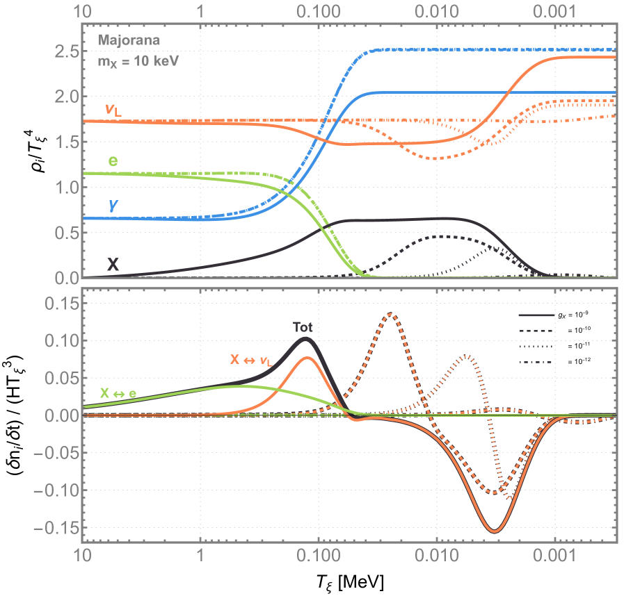
Figure 2: Top: The scaled density and bottom: and effective interaction rate for $m_{X}=10\,\text{keV}$ for couplings $g_{X}=10^{-9}$ (solid, $\Delta N_{\text{eff}}=2.2$), $g_{X}=10^{-10}$ (dashed, $\Delta N_{\text{eff}}=0.38$), $g_{X}=10^{-11}$ (dotted, $\Delta N_{\text{eff}}=0.29$), and $g_{X}=10^{-12}$ (dot-dashed, $\Delta N_{\text{eff}}=0.08$).

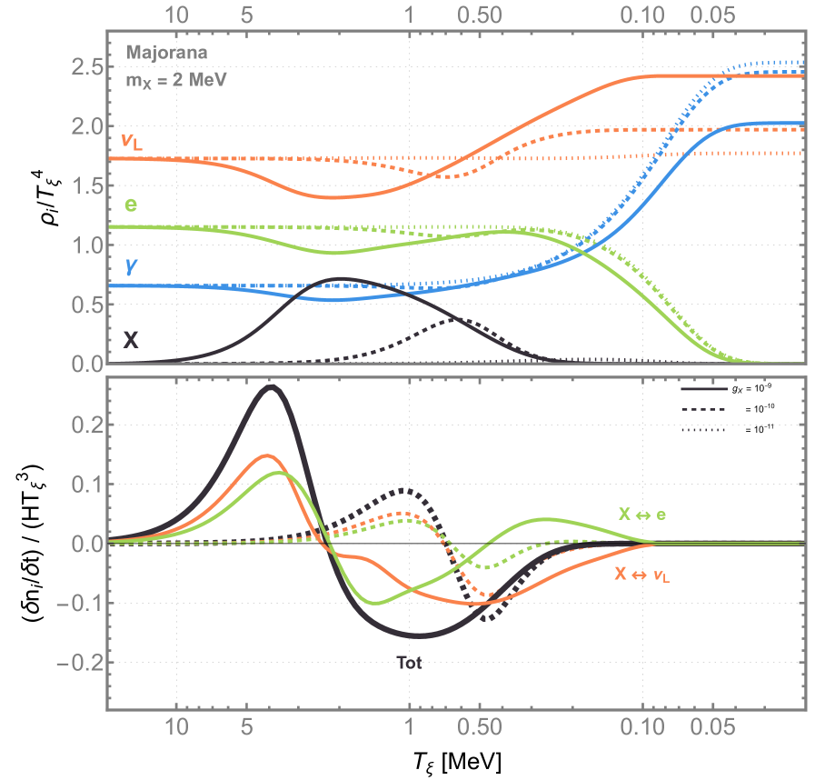
Figure 3: Top: The scaled density and bottom: and effective interaction rate for $m_{X}=2\,\text{MeV}$ for couplings $g_{X}=10^{-9}$ (solid, $\Delta N_{\text{eff}}=2.22$), $g_{X}=10^{-10}$ (dashed, $\Delta N_{\text{eff}}=0.49$), and in the upper figure only, $g_{X}=10^{-11}$ (dotted, $\Delta N_{\text{eff}}=0.03$).

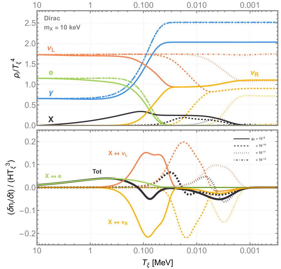
Figure 4: Top: The scaled density and bottom: and effective interaction rate for $m_{X}=10\,\text{keV}$ with Dirac neutrinos for couplings $g_{X}=10^{-9}$ (solid, $\Delta N_{\text{eff}}=1.75$), $g_{X}=10^{-10}$ (dashed, $\Delta N_{\text{eff}}=0.12$), $g_{X}=10^{-11}$ (dotted, $\Delta N_{\text{eff}}=0.12$), and in the upper figure only, $g_{X}=10^{-12}$ (dot-dashed, $\Delta N_{\text{eff}}=0.05$).

Next, for $g_{X}=10^{-9}$ as shown in Fig. 2, the coupling becomes strong enough for $\gamma X\leftrightarrow e^{+}e^{-}$ and $e^{\pm}X\leftrightarrow e^{\pm}\gamma$ to be efficient. Here, both electrons and neutrinos contribute to the population of $X$ with the electron interaction becoming efficient earlier. Note that the $X\leftrightarrow e$ effective interaction rate is always positive since $m_{e}>m_{X}$ and electron-positron annihilation occurs before $X$ decay. This means that the forward reactions ($\gamma X\rightarrow e^{+}e^{-}$ and $e^{\pm}X\rightarrow e^{\pm}\gamma$) never dominates over the backward reactions. So while electrons transfer their energy to $X$, the energy is never returned (unlike the case with neutrinos). This affects the evolution two-fold: (i) electron-positron annihilation dumps less entropy into photon plasma, decreasing $\rho_{\gamma}$; (ii) entropy stolen from electrons/positrons is later dumped into neutrinos, further increasing $\rho_{\nu}$. Both effects result in a larger value of $N_{\text{eff}}$.

In Fig. 3, we show the same plot for $m_{X}=2$ MeV. In this case, the $X\leftrightarrow e^{+}e^{-}$ process is active and the population of $X$ particles is depleted the decays of $X$s before electron-positron annihilation has completed. For $g_{X}=10^{-10}$, electrons and neutrinos populate a distribution of $X$ until $T_{\xi}\simeq 0.7$ MeV, then $X$ decay takes over and dumps its entropy back into both electrons and neutrinos. However for this mass, both $e^{\pm}$ and $X$ become non-relativistic and evolve as matter around roughly the same time. This means that the back and forth exchange in energy does not comparatively increase the energy density of electrons as it does for neutrinos. Another effect shown in Fig. 3 (lower) is the evolution of the effective $X\leftrightarrow e$ interaction rate from positive to negative, and then back to positive; this is most prominently shown in the $g_{X}=10^{-9}$ case. The first positive bump is the forward reaction $e^{+}e^{-}\rightarrow X$, followed by $X$ going nonrelativistic, with $X$ decaying into $e^{+}e^{-}$ and $\nu_{L}\bar{\nu}_{L}$, and then finally $e^{+}e^{-}\rightarrow X$ occurs on the Boltzmann tail of the electron distribution, and this small regenerated population of $X$ decays mostly back into neutrinos.

In Fig. 4, we show the evolution for $m_{X}=10$ keV with Dirac neutrinos. For low couplings, $\nu_{L}^{i}\bar{\nu}_{L}^{i}\rightarrow X$ populates $X$ and $X\rightarrow\nu_{R}^{i}\bar{\nu}_{R}^{i}$ populates right-handed neutrinos driving $X-{\nu_{L}}-{\nu_{R}}$ system into thermal equilibrium. The energy density of primordial left-handed neutrinos is now distributed among $X$, ${\nu_{L}}$, and ${\nu_{R}}$. Hence, the maximum energy density that $X$ can achieve is smaller than in the Majorana neutrino case. Increasing the coupling from $g_{X}=10^{-12}$ to $g_{X}=10^{-10}$ shows the trend towards thermalization of ${\nu_{L}}$ with ${\nu_{R}}$ as the interaction rate becomes efficient. For $g_{X}=10^{-10}$, the initial distribution of left-handed neutrinos has been converted to an equal distribution of left- and right-handed neutrinos. If this were to happen instantaneously, there would be no effect on $N_{\text{eff}}\propto(\rho_{\nu_{L}}+\rho_{\nu_{R}})/\rho_{\gamma}$. However, since this thermalization process generates an abundance of $X$, which then becomes nonrelativistic, evolves as matter, and then decays, there is an increase in $N_{\rm eff}$ just as occurred in the Majorana case in Fig. 2.

5.3 Numerical Results for $N_{\rm eff}$

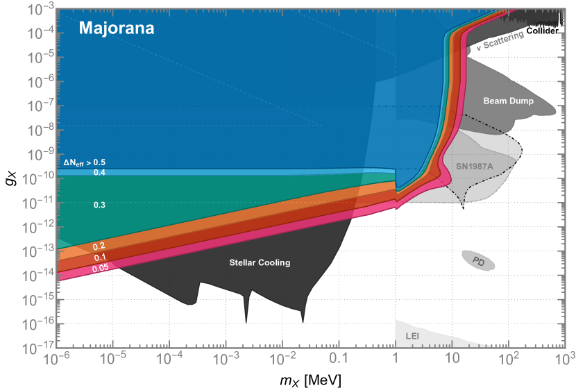
Figure 5: Calculations of $\Delta N_{\text{eff}}$ for the “Majorana” neutrino case. The regions correspond to $\Delta N_{\rm eff}>$ $0.05$ (pink), $0.1$ (red), $0.2$ (orange), $0.3$ (green), $0.4$ (light blue), and $0.5$ (dark blue). The dashed gray and dot-dashed black lines show the constraints from SN1987A from [76] and [77] respectively. See Sec. 5.4 for a discussion of SN1987A and other background constraints. Current constraints from Planck data exclude $\Delta N_{\text{eff}}\gtrsim 0.3$-$0.4$ (depending on the choice of dataset) [24], while future CMB observatories, such as CMB-S4, are expected to reach $\Delta N_{\text{eff}}\sim 0.06$ [67]. See Sec. 5.5 for further discussion of current and future constraints.

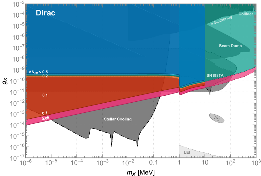
Figure 6: Same as Fig. 5, but for the “Dirac” neutrino case. As before, the regions correspond to $\Delta N_{\rm eff}>$ $0.05$ (pink), $0.1$ (red), $0.2$ (orange), $0.3$ (green), $0.4$ (light blue), and $0.5$ (dark blue). The dashed pink and green contours correspond to $\Delta N_{\text{eff}}=0.06\,\{0.3\}$ in [78] respectively. The dashed gray and dot-dashed black lines show the constraints from SN1987A from [76] and [77] respectively. See Sec. 5.4 for a discussion of SN1987A and other background constraints.

We now show the full results of our evaluation of $N_{\text{eff}}$ in the $(m_{X},g_{X})$ plane in Fig. 5 (Majorana neutrino case) and Fig. 6 (Dirac neutrino case).

Let’s first discuss the Majorana neutrino case, Fig. 5. This is a contour plot in $\Delta N_{\text{eff}}$, where colored regions provide our result for $\Delta N_{\text{eff}}$ as shown in the plot. In each colored region, $\Delta N_{\text{eff}}$ is greater than the value as shown, and less than its nearest neighboring region. For the dark blue region, $\Delta N_{\text{eff}}>0.5$, and we did not delineate any larger values, for reasons that we will discuss shortly.

There are three regimes of $m_{X}$ that reveal the qualitatively different processes that are occurring to determine the contribution to $\Delta N_{\text{eff}}$. In the low mass region, $m_{X}<2m_{e}$, with $\Delta N_{\text{eff}}\sim 0.05$ to $0.2$, the process $X\leftrightarrow\nu_{L}\bar{\nu}_{L}$ is approaching thermal equilibrium. The shape of the contour in $(m_{X},g_{X})$ space, $g_{X}\sim\sqrt{(24\pi m_{X})/M_{\text{Pl}}}$, can be obtained from $\Gamma_{X\leftrightarrow\nu_{L}\bar{\nu}_{L}}/H\sim 1$ and $T=m_{X}$. The precise value of $N_{\text{eff}}$ requires the numerical modeling of the Boltzmann evolution. (However, as we will see in Sec. 6, we can also estimate the value of $\Delta N_{\text{eff}}$ using semi-analytic arguments.) We see that in this region, the bounds on $g_{X}$ strengthen with decreasing $m_{X}$. Also in this region, there is a change in the shape of the $\Delta N_{\text{eff}}$ contours near $0.4$-$0.5$ that arises from $e^{+}e^{-}\rightarrow X\gamma$ becoming efficient near temperatures $T\simeq 2m_{e}$. Since this process depends on just $g_{X}$ (with $m_{X}<2m_{e}$), the contours are horizontal, approximately $g_{X}\sim\sqrt{2m_{e}/(\alpha M_{\text{Pl}})}\sim 10^{-10}$, independent of $m_{X}$.

In the intermediate mass region, $1\;{\rm MeV}\;\lesssim m_{X}\lesssim 20\;{\rm MeV}$, the contours in $\Delta N_{\text{eff}}$ rise rapidly in $g_{X}$ as $m_{X}$ increases. The major contributor to the rapid rise of $\Delta N_{\text{eff}}$ contours in $g_{X}$ as $m_{X}$ increases is that as $X$ becomes more massive, it becomes nonrelativistic earlier in the universe, and most of its decays back into SM matter occurs before neutrino decoupling. The SM processes rapidly equilibrate the relativistic species, erasing the effect of $X$ production and decay. There is detailed structure, such as the shape of the contours near $\Delta N_{\text{eff}}\sim 0.05$ and masses $m_{X}\sim 10$ MeV, that is a more complicated interplay between $X$, electrons, and neutrinos.

Finally, in high mass region, $m_{X}>20$ MeV, the Boltzmann evolution is calculated only involving photons, electrons, and neutrinos, with virtual $X$-exchange in the $2\leftrightarrow 2$ processes $e^{+}e^{-}\leftrightarrow\bar{\nu}_{\alpha}\nu_{\alpha}$, $e^{\pm}\nu_{\alpha}\leftrightarrow e^{\pm}\nu_{\alpha}$, and $e^{\pm}\bar{\nu}_{\alpha}\leftrightarrow e^{\pm}\bar{\nu}_{\alpha}$. The $\Delta N_{\text{eff}}$ contours in this region have a shape that can be determined by requiring $X$-exchange is no larger than $W$,$Z$ exchange. This occurs when $g_{X}\sim m_{X}\sqrt{G_{F}}$, providing an excellent characterization of the shape. The physics of this process is that if $X$ exchange exceeds the weak interaction rate, this delays neutrino decoupling in the evolution of the universe, which has the effect of increasing $\Delta N_{\text{eff}}$. Our contour shape agrees with that shown in [64].

Now, let’s discuss the contours in the Dirac neutrino case, Fig. 6, comparing and contrasting with the Majorana neutrino case. In the low mass region, $m_{X}<2m_{e}$, the shape of the $\Delta N_{\text{eff}}$ contours is the same as the Majorana case, with the only difference being that the contour values of $\Delta N_{\text{eff}}$ are somewhat lower. As we discussed in Sec. 5.2, what is happening is that the the energy density of primordial left-handed neutrinos is now distributed among $X$, ${\nu_{L}}$, and ${\nu_{R}}$. Hence, the maximum energy density that $X$ can achieve is smaller than in the Majorana case, and so the entropy dump of $X$ into neutrinos is smaller. Later in Sec. 6 we will verify this with a semi-analytic analysis. We also see that the constraint from $e^{+}e^{-}\rightarrow X\gamma$ becoming efficient near temperatures $T\simeq 2m_{e}$ remains.

At intermediate masses, $m_{X}\gtrsim 1$ MeV, as $X$ is populated, then becomes nonrelativistic, it decays into both left-handed and right-handed neutrinos. Hence, it contributes significantly to $\Delta N_{\rm eff}$ because $X$ is providing a mechanism to siphon off energy density from left-handed neutrinos into a “new” species, right-handed neutrinos, that are completely decoupled from the SM. This is unlike the Majorana case, where again for $m_{X}\gtrsim~{}{\rm few}$ MeV, $X$ decays back entirely into SM states that equilbriate with the SM through electromagnetic or weak interactions. This effect of populating right-handed neutrinos implies the contours in $\Delta N_{\text{eff}}$ are at much smaller values of $g_{X}$ when $m_{X}\gg 1$ MeV. We have calculated the result to $m_{X}=10$ MeV, and then we show the contours obtained by [78] for larger masses. In particular, the dashed pink and green contours, that correspond to $\Delta N_{\text{eff}}=0.06\,\{0.3\}$, match well onto our calculations for $m_{X}<10$ MeV.

There is one last issue to discuss. At the very smallest masses that we consider, the lifetime of $X$ becomes comparable to the time of recombination

$$\tau=\frac{c}{\Gamma} \simeq 330\;{\rm kyr}\times\left(\frac{1\;{\rm eV}}{m_{X}}\right)\left(\frac{4\times 10^{-14}}{g_{X}}\right)^{2}\,,$$ (27)

for the Majorana neutrino case (for the Dirac case the lifetime is $1/2$ of this). This means not all of the $X$ bosons that freeze-in have decayed back to relativistic neutrino degrees of freedom. This effect was taken into account in [58], in the context of a model with a $U(1)_{\mu-\tau}$ gauge boson. There, it was shown that the $\Delta N_{\text{eff}}$ constraint can be applied down to approximately $\mathcal{O}({\rm few}\;{\rm eV})$. Given that for $U(1)_{B-L}$, both the Majorana (Dirac) case we have a factor $3/2$ ($3$) more degrees of freedom to decay into, and so the lifetime is shorter by the same factor, the effects of the long lifetime of $X$ is not expected to shift our contours by any significant fraction.

5.4 Other Constraints

In Figs. 5,6, we have also shown several other constraints on the mass and coupling of a $U(1)_{B-L}$ gauge boson. An overview of previously obtained constraints can be found from [11, 12, 13, 14, 57].

Supernova 1987A (SN1987A) provides well-known constraints on the emission of light mediators [79]. The presence of a light vector mediator provides an additional cooling mechanism in the proto-neutron star that competes with electroweak interactions and alters its neutrino luminosity. Constraints on a variety of gauged $U(1)$ bosons have been derived in [80, 81, 77, 76]. The constraints for $U(1)_{B-L}$ in [77] and [76] are derived using slightly different methods and arrive at slightly different constraints. For completeness, we show both of these in the figures, and we will return to this issue in future work.

Similarly, constraints can be set if the energy loss rate due to light gauge boson emission from the sun, red giants (RG), and horizontal branch (HB) stars exceeds a maximally allowed limit [82, 81, 83]. Note both constraints from stellar cooling and SN1987A are derived explicitly for the case where right-handed neutrinos are heavy and do no contribute to the dynamics (“Majorana case”). To the best of our knowledge, a similar derivation has not been done in the literature for the Dirac case, though we do not suspect major differences in the results. So, we have included these constraints in Fig. 6, though denoted as dashed to remind the reader of this subtlety.

We also show the constraints from photodissociation (PD) of light elements, and separately, late energy injection (LEI) at the CMB era, that were obtained for $U(1)_{B-L}$ in [57]. These constraints are at much smaller coupling, where $X$ was very far from reaching thermal equilibrium, and for masses $m_{X}>2m_{e}$ so that the decay $X\rightarrow e^{+}e^{-}$ is kinematically available. In Figs. 5,6 we show only the upper part of the LEI contour; we refer readers to [57] for the full region that extends to couplings values $g_{X}<10^{-17}$.

Neutrino experiments that probe electron-neutrino or coherent elastic neutrino-nucleus scattering (CE$\nu$NS) are sensitive to the contribution of $X$ to their amplitudes [84, 85, 86, 87, 88, 89, 90, 91]. Experiments searching decays into invisible final states can also be used to set constraints with the assumption that invisible states can be treated as decays to neutrino final states [92, 93, 94, 95, 96]. In beam dump experiments [97, 98, 99, 100, 101, 102, 103, 104, 105, 106, 107], $X$ is produced via the bremsstrahlung process where a beam of electron/protons is dumped on some target material; $X$ then travels through shielding material before decaying into SM particles that can be observed in the detector. Constraints are derived by comparing the number of expected and observed events in the detector. Finally, colliders set constraints on promptly decaying $X$ [108, 109, 14]. These beam dump and collider constraints apply to both the Majorana and Dirac case. However in the Dirac case, collider and beam dump and neutrino scattering constraints have been recast to account for the additional branching fraction of $X\rightarrow\nu_{R}\bar{\nu}_{R}$ [12].

5.5 Constraints from Existing CMB Observations and Prospects for Future Observatories

We have presented our results in Figs. 5,6 with our calculated contours of $\Delta N_{\text{eff}}$ as would be measured by the CMB within the $(m_{X},g_{X})$ model parameter space. Determining the current and future constraints on $\Delta N_{\text{eff}}$ requires significant care with regard to two critical issues. First, the era at which new physics modifies $N_{\text{eff}}$, and what other cosmological parameters are also modified, particularly between BBN and CMB. Second, the datasets used to constrain the cosmological parameters, and the potential correlations among observables. In this section, our focus is on the CMB determination of $N_{\text{eff}}$.

Nevertheless, we can consider two proxies for BBN constraints on new physics that are potentially different from $N_{\text{eff}}$. One is the helium mass fraction $Y_{p}$, that we consider in detail in Sec. 7. A second quantity is the baryon-to-photon ratio, $\eta$. In general, new physics can contribute to a shifts in $\eta^{CMB}$ relative to $\eta^{BBN}$ when, for example, there is a period of late energy injection into photons well after the temperature of helium synthesis, $T\sim 0.07$ MeV [110, 27]. In the SM, there is negligible energy injection into photons at this temperature because $e^{+}e^{-}$ annihilation is virtually complete, and so $\eta^{CMB}\simeq\eta^{BBN}$. Considering $U(1)_{B-L}$, we also do not have late energy injection directly into photons. We do have energy injection into $e^{+}e^{-}$ from $X\rightarrow e^{+}e^{-}$, but since $e^{+}e^{-}$ annihilation did not affect $\eta$ in the SM, we do not expect these contributions from $X\rightarrow e^{+}e^{-}$ to shift $\eta$ from BBN to the CMB era either.

Focusing on $N_{\rm eff}^{\rm CMB}$, we can now turn to the current constraints and future prospects for cosmological measurements of $N_{\rm eff}^{\rm CMB}$. The Planck collaboration (PCP18) have set the best bounds thus far, with various combinations of datasets [23, 24]:

$$N_{\text{eff}}^{\text{CMB}}|^{\text{PCP18}}_{1\,\text{pe}} =2.99\,^{+0.34}_{-0.33}\; (95\%,\,\text{TT, TE, EE+lowE+ lensing+BAO})$$ (28a)

$$N_{\text{eff}}^{\text{CMB}}|^{\text{PCP18}}_{+Y_{p}} =2.99\,^{+0.43}_{-0.40}\; (95\%,\,\text{TT, TE, EE+lowE+ lensing+BAO+Aver \cite[cite]{[\@@bibref{}{Aver:2015iza}{}{}]}})$$ (28b)

$$N_{\text{eff}}^{\text{CMB}}|^{\text{PCP18}}_{+H_{0}} =3.27\,^{+0.30}_{-0.30}\; (95\%,\,\text{TT, TE, EE+lowE+ lensing+BAO+R18 \cite[cite]{[\@@bibref{}{Riess:2018uxu}{}{}]}}).$$ (28c)

The first value, $N_{\text{eff}}^{\text{CMB}}|^{\text{PCP18}}_{1\,\text{pe}}$, is the on 1-parameter extension to the base-$\Lambda\text{CDM}$ model six parameter fit. However, the primordial helium mass fraction $Y_{p}$ and $N_{\text{eff}}$ are partially degenerate as they both affect the CMB damping tail (i.e. [113]). Allowing $Y_{p}$ to vary with $N_{\text{eff}}$ gives a value of $N_{\text{eff}}^{\text{CMB}}|^{\text{PCP18}}_{+Y_{p}}$ and $Y_{p}^{\text{BBN}}|^{\text{PCP18}}_{+Y_{p}}=0.2437\,\pm 0.0080$ at $95\%$ C.L.. The combined fit eases the constraint on both $N_{\text{eff}}$ and $Y_{p}$ which has a PDG recommended value of $Y_{p}|^{\text{PDG}}=0.245\,\pm 0.006$ at $95\%$ C.L. [28] based on the analyses in [114, 115, 116, 117, 118]. Finally, the $N_{\text{eff}}^{\text{CMB}}|^{\text{PCP18}}_{+H_{0}}$ partially addresses the $\sim 3\sigma$ tension in the Hubble constant, $H_{0}$, between CMB and local observation determinations [112, 119, 120] by including the analysis in R18 [112]. This fit could potentially increase the tension with weak galaxy lensing and (possibly) cluster count data since it requires an increase in the $\sigma_{8}$ and a decrease in $\Omega_{m}$ values.

After the PCP18 data release and analysis, Yeh2022 [27] presents independent BBN and CMB limits on $N_{\text{eff}}$ and $\eta$ using likelihood analyses and updated evaluations for nuclear rates. The BBN likelihood functions are obtained by varying nuclear reaction rates within their uncertainties via a Monte Carlo, while the CMB likelihoods are derived from PCP18 and marginalized over $Y_{p}$. With various combinations of datasets,

$$N_{\text{eff}}^{\text{BBN}}|^{\text{Yeh2022}}_{\text{BBN only}} =2.889\,\pm\,0.229\; (68.3\%,Y_{p}+\text{D})$$ (29a)

$$N_{\text{eff}}^{\text{CMB}}|^{\text{Yeh2022}}_{\text{CMB only}} =2.800\,\pm\,0.294\; (68.3\%,\text{TT, TE, EE+lowE+ lensing})$$ (29b)

$$N_{\text{eff}}|^{\text{Yeh2022}}_{\text{BBN+CMB}} =2.898\,\pm\,0.141\; (68.3\%,\text{TT, TE, EE+lowE+ lensing}+Y_{p}+\text{D}).$$ (29c)

The first value, $N_{\text{eff}}^{\text{BBN}}|^{\text{Yeh2022}}_{\text{BBN only}}$, shows limits on $N_{\text{eff}}$ at BBN where the BBN likelihood is convolved with the observation determination of $Y_{p}$ and deuterium abundance D [121, 122, 123, 124, 125, 126, 127, 128] likelihoods. The second value, $N_{\text{eff}}^{\text{CMB}}|^{\text{Yeh2022}}_{\text{CMB only}}$, differs from Eq. (28a) as the Yeh2022 analysis does not assume any relation between the ${}^{4}\text{He}$ abundance and the baryon density. The third value is the limit set by combining BBN and the CMB assuming no new physics after nucleosynthesis, however this value is not applicable here since $X$ interactions can affect $\Delta N_{\text{eff}}$ between BBN and CMB.

Comparing these observations to our results, Figs. 5,6, a conservative analysis suggests $\Delta N_{\text{eff}}^{\rm CMB}\lesssim 0.3$-$0.4$ to 95% C.L., and hence the regions labeled dark and light blue are ruled out, with the green region strongly disfavored. If the ultimate resolution of the Hubble tension involves a slightly larger value of $N_{\text{eff}}^{\rm CMB}\simeq 3.27$, consistent with Eq. (28c), then the orange region is favored. Future observatories, including SPT-3G [129], CORE [130], Simons Observatory [131], PICO [132], CMB-S4 [67], CMB-HD [133], are anticipated to reach much smaller values, for example CMB-S4 is anticipated to ultimately obtain $\Delta N_{\text{eff}}\simeq 0.06$ at 95% C.L. [67]. Here we see these future experiments are capable of probing a significantly larger fraction of the $(m_{X},g_{X})$ parameter space in both the Majorana and Dirac neutrino cases. The future CMB observations will be the most sensitive to the presence of a gauged $U(1)_{B-L}$ boson in the regions $1\;{\rm eV}\lesssim m_{X}\lesssim 20\;{\rm eV}$, $0.2\;{\rm MeV}\lesssim m_{X}\lesssim 20\;{\rm MeV}$, and in the Dirac case, $m_{X}\gtrsim 200$ MeV [78].

6 Semi-Analytic Estimates of $\Delta N_{\text{eff}}$

There is an interesting way to cross-check our results in the regime $m_{X}\ll m_{e}$, where the only interactions of $X$ are with neutrinos. This semi-analytic approach involves two steps. First, we calculate the energy densities and number densities of $X$, assuming thermalization occurs at a temperature $T>m_{X}$. For the purposes of this estimate, we assume that thermalization occurs when $X$ is relativistic and can be treated as massless. The key nontrivial part of this first step is that we are solving for not only the energy densities but also the chemical potentials as $X$ is frozen-in to equilibrium with neutrinos. Next, we use entropy conservation to determine the net effect of $X$ decaying back into neutrinos. Again, this step is nontrivial because we also must take into account the nonzero chemical potentials of $X$ and the various neutrino species that (were) in equilibrium.

Given these assumptions, we are able to semi-analytically calculate the contribution to $\Delta N_{\rm eff}$. We now present the calculation in two regimes: first, the Majorana case, to get a clear sense of the method and its result. Next, the Dirac case, however we will generalize this to include an arbitrary number of additional species of (right-handed) fermions that carry lepton number. This case will allow us to provide semi-analytic estimates of $\Delta N_{\rm eff}$ in a wider range of models that may be relevant for dark matter and cosmology.

6.1 Majorana Case

An initial density of left-handed neutrinos with temperature $T_{\nu_{L}}$ is converted to a density of left-handed neutrinos and $X$,

$$\rho_{\nu_{L}}(T_{\nu_{L}},0) = \rho_{\nu_{L}}(T_{\text{eq}},\mu_{\text{eq}})+\rho_{X}(T_{\text{eq}},2\mu_{\text{eq}})$$ (30a)

$$n_{\nu_{L}}(T_{\nu_{L}},0) = n_{\nu_{L}}(T_{\text{eq}},\mu_{\text{eq}})+2n_{X}(T_{\text{eq}},2\mu_{\text{eq}}),$$ (30b)

with $T_{\text{eq}},\mu_{\text{eq}}$ thermal equilibrium temperature and chemical potential. In the second equation, the factor of $2$ arises because one $X$ is produced at the expense of two neutrinos in $\nu_{L}^{i}\bar{\nu}_{L}^{i}\rightarrow X$. These conditions give,

$$T_{\text{eq}}=1.208\,T_{\nu_{L}}\;,\quad\quad\mu_{\text{eq}}=-1.166\,T_{\nu_{L}}$$ (31)

which gives a maximum density ratio $\varrho_{X}\equiv\rho_{X}/(\rho_{\nu_{L}}+\rho_{X})=0.1642$. Had we neglected chemical potential, Eq. (30a) becomes a degree of freedom counting argument which yields $\varrho_{X}=3/(6\times\frac{7}{8}+3)=\frac{4}{11}=0.3636$ significantly overestimating the maximum $X$ abundance. Instead, the chemical potential appears as $\varrho_{X}=3\,\text{Li}_{4}(x)/[6\,\text{Li}_{4}(-x)+3\,\text{Li}_{4}(x)]$ with $x\equiv e^{\mu/T}$ and $\,\text{Li}_{4}$ is the $4^{\text{th}}$ order polylogarithm.

After thermal equilibrium is reached, we use entropy conservation to write,

$$\left[s_{\nu_{L}}(T_{\text{eq}},\mu_{\text{eq}})+s_{X}(T_{\text{eq}},2\mu_{\text{eq}})\right]a^{\prime 3} = s_{\nu_{L}}(T_{\nu},\mu_{\nu})a^{3}$$ (32a)

$$\left[n_{\nu_{L}}(T_{\text{eq}},\mu_{\text{eq}})+2n_{X}(T_{\text{eq}},2\mu_{\text{eq}})\right]a^{\prime 3} = n_{\nu_{L}}(T_{\nu},\mu_{\nu})a^{3}.$$ (32b)

The left-hand side starts at scale factor $a^{\prime}$ with equilibrium abundance of all relevant particles, while the right-hand side ends at a scale factor $a$ with $T_{\nu}\ll m_{X}$, where the entire distribution of $X$ bosons has decayed into neutrinos. We can relate the scale factors through $T_{\gamma}^{\prime}a^{\prime}=T_{\gamma}a$, since the photon plasma is decoupled from neutrinos. Solving Eq. (32) gives,

$$T_{\gamma}/T_{\nu}=1.278\,,\quad\quad T_{\nu}/\mu_{\nu}=-3.486$$ (33)

which can be used to calculate

$$\Delta N_{\text{eff}}=N_{\text{eff}}-N_{\text{eff}}^{\text{SM}}=0.25\,.$$ (34)

As we discussed in Sec. 5.3, the diagonal contours of $\Delta N_{\text{eff}}$ in the light regime $m_{X}\ll 2m_{e}$ correspond to when the $1\leftrightarrow 2$ process $X\leftrightarrow\nu\bar{\nu}$ approximately reaches thermal equilibrium. The highest contour shown is $0.3$, that is quite close to our semi-analytic estimate Eq. (34). Of course the semi-analytic method required certain approximations to be taken. Namely, in solving Eq. (32) we used the SM value of $T_{\gamma}/T_{\nu}$ in Eq. (10) to relate the scale factors $T_{\gamma}^{\prime}a^{\prime}=T_{\gamma}a$; and using the numerical value obtaining by solving the Boltzmann equations in Eq. (4.2) reproduces the correct value of $\Delta N_{\text{eff}}$.

6.2 Dirac and Generalized Cases

We now redo the analysis of Sec. 6.1 by adding into the thermal bath an arbitrary number $N_{R}$ of (Weyl) fermion species. As a slight abuse of notation, we will refer to these fermions as “right-handed neutrinos” below, but it should be understood that these fermion fields have $L=\pm 1$ and may or may not pair up with the left-handed neutrinos to gain Dirac masses. All of these right-handed neutrinos will be considered to be either (i) massless, or (ii) having a mass $m_{\nu_{R}}\lesssim m_{X}/2$. The Dirac case follows as a special case of this generalization where $N_{R}=3$, $m_{\nu_{R}}=0$, and two (or three) of these fermion species pair up with left-handed neutrinos.

Following Eqs. (30), an initial density of left-handed neutrinos with temperature $T_{\nu_{L}}$ is converted to a energy (number) density of left- and right-handed neutrinos [denote collectively by $\rho_{\nu}$ ($n_{\nu}$)] and $X$,

$$\rho_{\nu_{L}}(T_{\nu_{L}},0) = \left(1+\frac{N_{R}}{3}\right)\rho_{\nu}(T_{\text{eq}},\mu_{\text{eq}})+\rho_{X}(T_{\text{eq}},2\mu_{\text{eq}})$$ (35a)

$$n_{\nu_{L}}(T_{\nu_{L}},0) = \left(1+\frac{N_{R}}{3}\right)n_{\nu}(T_{\text{eq}},\mu_{\text{eq}})+2n_{X}(T_{\text{eq}},2\mu_{\text{eq}})$$ (35b)

with $T_{\text{eq}},\mu_{\text{eq}}$ thermal equilibrium temperature and chemical potential.

After thermal equilibrium is reached, we can again utilize entropy conservation to write,

$$\left[\left(1+\frac{N_{R}}{3}\right)s_{\nu}(T_{\text{eq}},\mu_{\text{eq}})+s_{X}(T_{\text{eq}},2\mu_{\text{eq}})\right]a^{\prime 3} = \left[\left(1+\frac{N_{R}}{3}\right)s_{\nu}(T_{\nu},\mu_{\nu})\right]a^{3}$$ (36a)

$$\left[\left(1+\frac{N_{R}}{3}\right)n_{\nu}(T_{\text{eq}},\mu_{\text{eq}})+2n_{X}(T_{\text{eq}},2\mu_{\text{eq}})\right]a^{\prime 3} = \left[\left(1+\frac{N_{R}}{3}\right)n_{\nu}(T_{\nu},\mu_{\nu})\right]a^{3}\,.$$ (36b)

Again, the left-hand side starts at scale factor $a^{\prime}$ with equilibrium abundance of all relevant particles and the right-hand side ends at scale factor $a$ with $T_{\nu}\ll m_{X}$ where all $X$ distribution has decayed into neutrinos.

6.2.1 Dirac case

In the Dirac case ($N_{R}=3$; $m_{\nu_{R}}=0$), Eqs. (35) give

$$T_{\text{eq}}=1.1088\,T_{\nu_{L}}\,,\quad\quad\mu_{\text{eq}}=-1.3485\,T_{\nu_{L}}\quad\quad\mbox{(Dirac case)}$$ (37)

which gives a maximum density ratio $\varrho_{X}\equiv\rho_{X}/(\rho_{\nu_{L}}+\rho_{X}+\rho_{\nu_{R}})=0.07049$. (Again, had we neglected chemical potential, Eq. (35a) becomes $\varrho_{X}=3/(12\times\frac{7}{8}+3)=\frac{2}{9}=0.2222$, overestimating the maximum $X$ abundance.) Solving Eq. (36) gives,

$$T_{\gamma}/T_{\nu}=1.322\,,\quad\quad T_{\nu}/\mu_{\nu}=-1.093\quad\quad\mbox{(Dirac case)}$$ (38)

which can be used to calculate

$$\Delta N_{\text{eff}}=N_{\text{eff}}-N_{\text{eff}}^{\text{SM}}=0.09\,.$$ (39)

Like our discussion above in the Majorana case, in Fig. 6 the highest contour consistent with approximate thermalization of $X\leftrightarrow\nu\bar{\nu}$ is $0.1$, that agrees with the semi-analytic estimate Eq. (39).

6.2.2 Large Number of Massless Species

Now let’s utilize the generalized results in Eqs. (35) and (36) to apply to the case where there is a large number of massless species $N_{R}\gg 1$ that $X$ can decay into. Once $X$ and the $1+N_{R}/3$ neutrinos have thermalized, it is clear from Eqs. (35) that the energy and number density of $X$ is suppressed by the same factor, $1/(1+N_{R}/3)$. Most of the energy and number density of left-handed neutrinos is transferred into the larger number of right-handed neutrinos. Then, following Eqs. (36), the effect of the small number of $X$ gauge bosons is negligible. That is, in the limit $N_{R}\gg 1$, there is negligible entropy dumping of $X$ into neutrinos, and so $\Delta N_{\rm eff}\rightarrow 0$. For smaller values of $N_{R}$, we find, for example $\Delta N_{\text{eff}}=0.12$ ($N_{R}=2$), $\Delta N_{\text{eff}}=0.07$ ($N_{R}=4$) and $\Delta N_{\text{eff}}=0.03$ ($N_{R}=8$). Here we do need to emphasize that while the number of relativistic degrees of freedom nearly matches the SM, the flavor of these degrees of freedom is overwhelmingly in the form of the (sterile) neutral fermion species carrying lepton number.

6.2.3 Massive Species

An alternative scenario occurs if the $N_{R}$ species are massive, and thus are able to annihilate through $X$ back into (massless) left-handed neutrinos species. Here what happens is that the large entropy of the right-handed neutrinos siphons off virtually all of the entropy in left-handed neutrinos. In the limit $N_{R}\gg 1$, with $m_{\nu_{R}}\lesssim m_{X}/2$, the overwhelming majority of the original energy density of left-handed neutrinos end up as nonrelativistic, massive (sterile) neutral fermion species. This leaves a negligible amount of left-handed neutrinos, and so in this limit, $\Delta N_{\rm eff}\rightarrow-3$, i.e., $N_{\rm eff}\rightarrow 0$. As a few examples where all $N_{R}$ species are massive, we find $\Delta N_{\text{eff}}=-0.64$ ($N_{R}=1$), $\Delta N_{\text{eff}}=-1.15$ ($N_{R}=2$) and $\Delta N_{\text{eff}}=-1.48$ ($N_{R}=3$). Notice that $N_{R}\geq 1$ is already completely excluded by the Planck constraints on the CMB, i.e., Eq. (28).

7 BBN $Y_{p}$

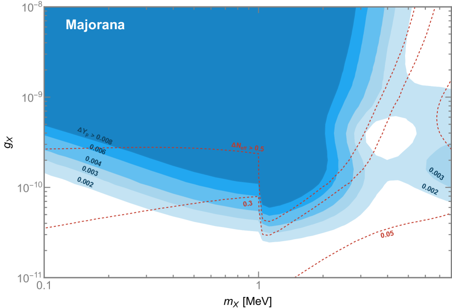
Figure 7: $\Delta Y_{p}$ contours for “Majorana” neutrino case. The dashed red lines show the contours from our calculation of $\Delta N_{\rm eff}$ observed by the CMB, from Fig. 5. A conservative upper bound is $\Delta Y_{p}=0.008$ at $95\%$ C.L. [27], see Sec. 7 for further discussion.

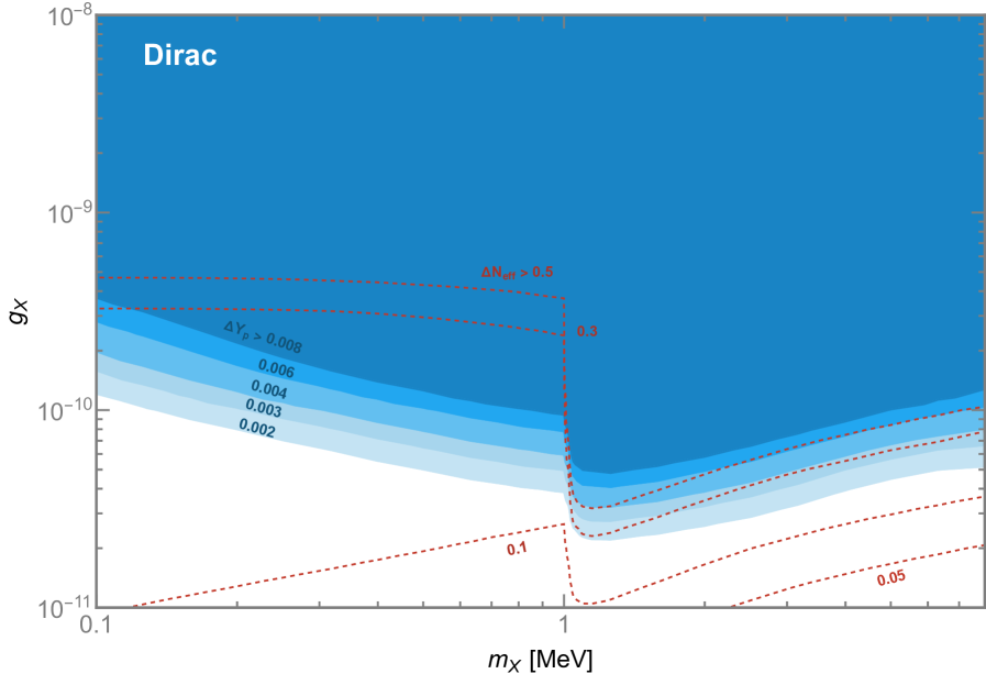
Figure 8: Same as Fig. 7, but for the “Dirac” neutrino case. The dashed red lines show the contours from our calculation of $\Delta N_{\rm eff}$ observed by the CMB, from Fig. 6.

The primordial abundances of nuclide species are critically sensitive to the expansion history leading up to nucleosynthesis. Precise determinations of these abundances requires solving Boltzmann equations describing the density evolution of each nuclide species $({}^{2}\text{H},{}^{3}\text{He},{}^{4}\text{He}...)$ (i.e. [42]). This can be done using publicly available BBN code such as PArthENoPE [134, 135], AlterBBN [136, 137], or PRIMAT [138]; however, this is beyond the scope of this paper.

Instead, we follow an approximation employed in Appendix A.4 of [54], that involves modifying the neutron-to-proton conversion rate to include a neutrino chemical potential following the derivation in [32, 34]. The Boltzmann equation describing the evolution of neutron fraction $X_{n}=\frac{n_{n}}{n_{n}+n_{p}}$ is [41]:

$$\frac{dX_{n}}{dt} =\Gamma_{pn}(1-X_{n})-\Gamma_{np}X_{n},$$ (40a)

$$\Gamma_{np} =K\int_{1}^{\infty}d\epsilon\left[\frac{(\epsilon-q)^{2}(\epsilon^{2}-1)^{1/2}\epsilon}{(1+e^{-\epsilon z_{\gamma}})(1+e^{(\epsilon-q-\tilde{\mu}_{\nu})z_{\nu}})}+\frac{(\epsilon+q)^{2}(\epsilon^{2}-1)^{1/2}\epsilon}{(1+e^{\epsilon z_{\gamma}})(1+e^{-(\epsilon-q-\tilde{\mu}_{\nu})z_{\nu}}}\right],$$ (40b)

$$\Gamma_{pn} =\Gamma_{np}(-q),$$ (40c)

where $z_{i}=m_{e}/T_{i}$, $\tilde{\mu}_{\nu}=\mu_{\nu}/m_{e}$, $q=(m_{n}-m_{p})/m_{e}$, and $K\simeq(1.939\tau_{n})^{-1}$. We take $m_{n}-m_{p}=1.2933$ MeV and neutron lifetime $\tau_{n}=878.4$ s [28]. Here $\Gamma_{np}$ is the rate for neutron to proton conversion through the weak interactions $n+\nu_{e}\leftrightarrow p+e^{-}$, $n+e^{+}\leftrightarrow p+\bar{\nu}_{e}$, and $n\leftrightarrow p+e^{-}+\bar{\nu}_{e}$. The evolution of $T_{\gamma},\,T_{\nu}$ and $\mu_{\nu}$ are obtained separately, by solving Eq. (4.2) as described in Sec. 4.2. To estimate the helium abundance $Y_{p}$, we take the limit where all remaining neutrons form helium around the temperature where photons no longer dissociate deuterium $T_{D}=0.073$ MeV; in other words,

$$Y_{p}\simeq 2X_{n}|_{T=T_{D}}\,.$$ (41)

In the SM, applying this procedure yields $Y_{p}|^{\text{Eq. }\ref{YpEqn}}_{\text{SM}}=0.248$ in agreement with $Y_{p}|^{\text{PDG}}=0.245\,\pm 0.006$ at $95\%$ C.L. [28]. We define the BSM deviation of helium abundance as

$$\Delta Y_{p}=Y_{p}|^{\text{Eq. }\ref{YpEqn}}_{\text{BSM}}-Y_{p}|^{\text{Eq. }\ref{YpEqn}}_{\text{SM}}.$$ (42)

The $\Delta Y_{p}$ contours for the Majorana and Dirac case are shown in Figs. 7,8, along with overlays of the respective $\Delta N_{\text{eff}}$ contours in red. In accordance with the discussion in Sec. 5.5, a conservative upper bound is $\Delta Y_{p}=0.008$ at $95\%$ C.L. In both the Majorana and Dirac cases, $\Delta N_{\text{eff}}$ constraints are stronger for $m_{X}>2m_{e}$. However, in the Dirac case, we find $\Delta Y_{p}>0.008$ in the mass region $0.1\;{\rm MeV}\lesssim m_{X}\lesssim 2m_{e}$, where the Planck constraint from the CMB, $\Delta N_{\text{eff}}\lesssim 0.3$ is currently weaker. Once the future CMB observatories reach $\Delta N_{\text{eff}}\lesssim 0.15$, their constraints will exceed what can be set by this analysis of BBN.

8 Discussion

In this paper we calculated the contributions of a light $U(1)_{B-L}$ gauge boson mediator to $\Delta N_{\rm eff}$ as measured by the CMB and $Y_{p}$ from BBN. Our main result is Figs. 5,6, where we show our predictions for $\Delta N_{\rm eff}$ as a function of of the $U(1)_{B-L}$ gauge boson mass $m_{X}$ and coupling strength $g_{X}$, along with Figs. 7,8 where we show our predictions for the shift in the helium mass fraction $\Delta Y_{p}$, in the same parameter space. While substantial portions of the ($m_{X}$, $g_{X}$) parameter space have overlapping constraints from other astrophysical or terrestrial experiments, we find there are several regions where future CMB observatories [129, 130, 131, 132, 67, 133], have the opportunity to gain sensitivity to a very weakly coupled $U(1)_{B-L}$ gauge boson in certain mass and coupling ranges that is not accessible by any other method.

We have also calculated $\Delta Y_{p}$, the helium abundance, which serves as a proxy for $\Delta N_{\rm eff}$ as observed by BBN. This result utilized an approximation from Ref. [54] to estimate the change in the helium abundance that follows from a nonzero neutrino chemical potential, as occurs with a freeze-in abundance of a $U(1)_{B-L}$ gauge boson. In Fig. 7, we find that for the Majorana case, the Planck constraints on the CMB are generally stronger than the BBN constraints on $Y_{p}$ throughout the $(m_{X},g_{X})$ plane. For the Dirac case shown in Fig. 8, however, there is a nontrivial region of parameter space (approximately $0.1\;{\rm MeV}\lesssim m_{X}\lesssim 1~{}{\rm MeV}$, $g_{X}\lesssim 4\times 10^{-9}$), where the BBN constraints are stronger than the constraints from $\Delta N_{\rm eff}$ from Planck data. However, future CMB observatories [129, 130, 131, 132, 67, 133], will be able to fully cover this region, and probe considerably smaller couplings, once they achieve $\Delta N_{\rm eff}\lesssim 0.15$ sensitivity.

We also considered semi-analytic estimates of our $\Delta N_{\rm eff}$ results. Our focus for these estimates was the region $m_{X}\ll 2m_{e}$, where the only species interacting with $X$ are neutrinos. The semi-analytic estimates allow us to obtain an approximate value for $\Delta N_{\rm eff}$ in the region $m_{X}\ll 2m_{e}$. In this region, $X$ approaches thermal equilibrium with neutrinos. The reason our contours of $\Delta N_{\rm eff}$ are parallel lines that strengthen as $g_{X}$ is increased can be understood as the $X$ bosons achieving “asymptotic thermal equilibrium”. By this we mean that the $X$ bosons would have achieved thermal equilibrium had they not decayed. Said differently, holding $g_{X}$ fixed, as $m_{X}$ is increased, we quickly encounter the smaller contours in $\Delta N_{\rm eff}$ because a smaller fraction of $X$ bosons live long enough to achieve thermal equilibrium with neutrinos.

The semi-analytic estimates also permit us to determine how our results change if there are additional degrees of freedom, beyond the SM, that the $X$ boson is able to populate. The physical picture is that $X$ slowly freezes in, becomes nonrelativistic, and then decays into SM states plus the additional degrees of freedom beyond the SM. For this analysis, we considered a set $N_{R}$ of fermions carrying lepton number (right-handed neutrinos with $L=\pm 1$), in two scenarios: the additional fermions stay relativistic (at least until recombination), or the additional fermions have masses and become nonrelativistic matter. If the fermions stay relativistic, $\Delta N_{\rm eff}\rightarrow 0$ as $N_{R}$ becomes large, essentially because they dominate the relativistic degrees of freedom after entropy equilibration. On the other hand, if they become nonrelativistic before recombination, they siphon off most of the relativistic degrees of freedom into matter, and so $N_{\rm eff}\rightarrow 0$ ($\Delta N_{\rm eff}\rightarrow-3$).

Our results have interesting implications on other scenarios considered in the literature:

Ref. [139] considered light new vectors produced gravitationally during inflation that also couple to neutrinos. The coupling to neutrinos imply the inflationary produced vector can decay into neutrinos, giving additional contributions to $\Delta N_{\rm eff}$, that led to constraints in the $(m_{X},g_{X})$ plane. These contributions to $\Delta N_{\rm eff}$ rely on a primordial abundance of vector bosons from inflation, and thus constitute a contribution that is in addition to the freeze-in abundance of a massive vector that couples to neutrinos. On comparing our bounds to those from [139], we find our constraints would appear to place significant restrictions on the scale of inflation and hence the inflationary production of vector bosons that couple to neutrinos.

One of the additional effects of a light $X$ boson, with a mass well below the neutrino decoupling temperature, $m_{X}\ll 2$ MeV, is that the interactions with $X$ can suppress the free streaming of neutrinos, and this has independent constraints from the suppression of small scale structure [140] that results in shifts in the phase and a decrease in the amplitude of the acoustic peaks of the CMB [141, 52, 142, 143]. Recently, [58] analyzed the suppression of neutrino free streaming resulting from neutrino interactions within the context of a model with a very light $U(1)_{\mu-\tau}$ gauge boson. By implementing these interactions into the modeling of the CMB, they were able to use Planck data to constrain a broad range of $U(1)_{\mu-\tau}$ gauge boson masses between $10^{-3}$ eV to $10^{3}$ eV, with the strongest bound on $g_{\mu-\tau}$ near $1$ eV, and rapidly decreasing bounds as the mass moved away from this value. Nevertheless, for masses $1$ eV and larger, [58] found that the bounds from $\Delta N_{\rm eff}$ are still stronger than those from the suppression of the free streaming of neutrinos. This is strongly suggestive that the bounds from $\Delta N_{\rm eff}$ are very likely stronger than constraints from the suppression of neutrino free streaming in the model considered in this paper, $U(1)_{B-L}$, though we leave a detailed analysis of this point to future work.

Several other papers have considered a light $U(1)_{B-L}$ gauge boson’s effects in various contexts. For example, our work complements and extends the analysis of [12] and [78], who considered bounds on a $U(1)_{B-L}$ model in which neutrinos acquire Dirac masses. Our work rules out substantial parts of previously allowed parameter space in [144], who considered constraints on $U(1)_{B-L}$ from neutrino-electron and neutrino-nucleon scattering. As can be seen in Fig. 5, the remaining region that is more strongly constrained by neutrino-nucleon scattering occurs only when $m_{X}\gtrsim 10$ MeV in the Majorana case. By contrast, when neutrinos have Dirac masses, the CMB constraints completely dominate the bounds even at larger masses as shown in Fig. 6 (that includes the results from [78]). Ref. [145] considered sterile neutrino dark matter arising from interactions with $U(1)_{B-L}$. While our analysis of the CMB constraints does not rule out the main region favored by [145], essentially all of their parameter space $m_{X}\lesssim 10$ MeV would be in conflict with the CMB that extends and compliments the existing constraints from beam dump experiments.

Beyond $U(1)_{B-L}$, there has also been extensive discussion of equilibration of a dark sector with neutrinos well after BBN [146, 147, 110]. The motivation of this work is to obtain thermal dark matter below an MeV [146, 147]. There are commonalities between this work and ours, specifically the observation that if a light state couples only to neutrinos, equilibration with neutrinos draws heat from the SM, and only after the species decouples, the neutrino bath is heated, contributing to $\Delta N_{\text{eff}}$. The distinction between our work and [146, 147, 110] is that we find the Boltzmann equations require the presence of a nonzero chemical potential for $X$ as well as neutrinos, in order to properly track the evolution of the energy densities of the various species, and therefore to accurately calculate $\Delta N_{\text{eff}}$. For instance, when our $X$ boson can decay into just one massive species (one massive “sterile” Majorana neutrino), this siphons off a sufficient amount of entropy from the left-handed neutrinos of the SM to already be excluded by Planck data. It would be very interesting to apply our analysis to the specific scenarios of [146, 147], to determine if including a chemical potential for the mediators and DM has an effect on the results, but we leave for future work.

Note added: As this work was being completed [148] appeared that also discussed the bounds on a model with a light $U(1)_{B-L}$ (with Majorana neutrino masses) and $U(1)_{\mu-\tau}$ boson from $\Delta N_{\rm eff}$. Among the differences between their work and ours, we include the coupling of the $U(1)_{B-L}$ mediator to charged leptons (electrons), and the associated $1\leftrightarrow 2$, $2\leftrightarrow 2$ processes that are essential to determining the effects on $\Delta N_{\text{eff}}$ for temperatures near and above BBN.

Appendix A Right-handed Neutrino Decay in Majorana Case

In the regime $M_{R}>m_{h}+m_{\nu}$, the 2-body decay is rapid, and the right-handed neutrinos will have completely decayed well prior to BBN. When $M_{R}<m_{h}$, the decay is 3-body, with an off-shell Higgs that will also be suppressed by the small Yukawa coupling $y_{\rm SM}$ of the Higgs to lighter SM fermions. An estimate of this 3-body width to one SM fermion pair is sufficient for our purposes,

$$\Gamma(\nu_{R}\rightarrow\nu_{L}f\bar{f}) \sim \frac{y_{D}^{2}y_{\rm SM}^{2}M_{R}^{5}}{128\pi^{3}m_{h}^{4}}\,,$$ (43)

where we have neglected the final state phase space. If a SM neutrino species has a mass $m_{\nu}\sim(y_{D}v)^{2}/M_{R}$, the width becomes

$$\Gamma(\nu_{R}\rightarrow\nu_{L}f\bar{f}) \sim \frac{m_{\nu}y_{\rm SM}^{2}M_{R}^{6}}{128\pi^{3}v^{2}m_{h}^{4}}$$ (44)

leading to a lifetime

$$\tau(\nu_{R}\rightarrow\nu_{L}f\bar{f}) \sim (1\;{\rm s})\times\left(\frac{10\;{\rm GeV}}{M_{R}}\right)^{6}\times\left(\frac{0.1\;{\rm eV}}{m_{\nu}}\right)\times\left(\frac{y_{b}}{y_{\rm SM}}\right)^{2}\,,$$ (45)

where we have normalized the Yukawa coupling $y_{\rm SM}$ to the $b$-quark Yukawa coupling. If $M_{R}\gtrsim 2m_{b}$, we expect $\nu_{R}$ to decay predominantly a $b\bar{b}$ pair since this is the heaviest SM fermions that are kinematically available for the 2-body decay. If $M_{R}$ is slightly less than the $2m_{b}$ threshold, decays to $c\bar{c}$ and $\tau^{+}\tau^{-}$ would be present, with $y_{\rm SM}$ slightly smaller than $y_{b}$.

In any case, the above estimate demonstrates that for $M_{R}\lesssim 10$ GeV, $\nu_{R}$ are comparatively long-lived and can disrupt BBN light element abundance predictions due to the electromagnetic energy deposition [149]. Given that the width, Eq. (44), depends on the 6th power of $M_{R}$, one only needs slightly larger masses, $M_{R}\gtrsim 20$ GeV, to cause $\nu_{R}$ to decay sufficiently fast to completely avoid BBN constraints.

This leads to two possibilities in the Majorana scenario:

If $\nu_{R}$ was in thermal equilibrium in the early Universe, $M_{R}\gtrsim 20$ GeV is required to avoid BBN constraints, and thus $v_{X}\gtrsim(20\;{\rm GeV})/y_{M}$. If $X^{\mu}$ acquires all of its mass from just the $\phi_{X}$ vev, then $m_{X}$ is determined once $g_{X}$ is specified, specifically, $m_{X}=2g_{X}v_{X}$. The scalar Higgs sector of $U(1)_{B-L}$ need not be minimal. There could be other scalars with $B-L$ charge that differ $\phi_{X}$, i.e., $\phi_{X^{\prime}}$ with $q_{X^{\prime}}\not=\pm 2$. These do not lead to contributions to the Majorana masses, but will lead to an additional contribution to the $X^{\mu}$ gauge boson mass, $m_{X}^{2}=g_{X}^{2}\left(4v_{X}^{2}+q_{X^{\prime}}^{2}v_{X^{\prime}}^{2}\right)$. Hence, we see that the minimal case $m_{X}=2g_{X}v_{X}$ is a lower bound on $m_{X}$ for a generic $U(1)_{B-L}$ breaking sector. Said directly, the bound $M_{R}\gtrsim 20$ GeV implies

$$g_{X} < \frac{m_{X}}{2v_{X}}$$ (46)

$$\lesssim 2.5\times 10^{-5}\frac{m_{X}}{1\;{\rm MeV}}\qquad\mbox{(if $\nu_{R}$ in early thermal equilibrium).}$$

On the other hand, it could be that $\nu_{R}$ was never in thermal equilibrium in the early universe. In this case, no population of $\nu_{R}$’s were generated, and there is no bound on $g_{X}$ from $\nu_{R}$ decay.

References

- [1] J. Alexander et al., “Dark Sectors 2016 Workshop: Community Report,” 8, 2016. arXiv:1608.08632 [hep-ph].
- [2] M. Battaglieri et al., “US Cosmic Visions: New Ideas in Dark Matter 2017: Community Report,” in U.S. Cosmic Visions: New Ideas in Dark Matter. 7, 2017. arXiv:1707.04591 [hep-ph].
- [3] N. Arkani-Hamed, D. P. Finkbeiner, T. R. Slatyer, and N. Weiner, “A Theory of Dark Matter,” Phys. Rev. D 79 (2009) 015014, arXiv:0810.0713 [hep-ph].
- [4] M. Pospelov and A. Ritz, “Astrophysical Signatures of Secluded Dark Matter,” Phys. Lett. B 671 (2009) 391–397, arXiv:0810.1502 [hep-ph].
- [5] M. Pospelov, “Secluded U(1) below the weak scale,” Phys. Rev. D 80 (2009) 095002, arXiv:0811.1030 [hep-ph].
- [6] M. Fabbrichesi, E. Gabrielli, and G. Lanfranchi, “The Dark Photon,” arXiv:2005.01515 [hep-ph].
- [7] R. E. Marshak and R. N. Mohapatra, “Quark - Lepton Symmetry and B-L as the U(1) Generator of the Electroweak Symmetry Group,” Phys. Lett. B 91 (1980) 222–224.
- [8] R. N. Mohapatra and R. E. Marshak, “Local B-L Symmetry of Electroweak Interactions, Majorana Neutrinos and Neutron Oscillations,” Phys. Rev. Lett. 44 (1980) 1316–1319. [Erratum: Phys.Rev.Lett. 44, 1643 (1980)].
- [9] C. Wetterich, “Neutrino Masses and the Scale of B-L Violation,” Nucl. Phys. B 187 (1981) 343–375.
- [10] P. Langacker, “The Physics of Heavy Gauge Bosons,” Rev. Mod. Phys. 81 (2009) 1199–1228, arXiv:0801.1345 [hep-ph].
- [11] R. Harnik, J. Kopp, and P. A. N. Machado, “Exploring nu Signals in Dark Matter Detectors,” JCAP 07 (2012) 026, arXiv:1202.6073 [hep-ph].
- [12] J. Heeck, “Unbroken B – L symmetry,” Phys. Lett. B 739 (2014) 256–262, arXiv:1408.6845 [hep-ph].
- [13] M. Bauer, P. Foldenauer, and J. Jaeckel, “Hunting All the Hidden Photons,” JHEP 07 (2018) 094, arXiv:1803.05466 [hep-ph].
- [14] P. Ilten, Y. Soreq, M. Williams, and W. Xue, “Serendipity in dark photon searches,” JHEP 06 (2018) 004, arXiv:1801.04847 [hep-ph].
- [15] A. E. Nelson and N. Tetradis, “CONSTRAINTS ON A NEW VECTOR BOSON COUPLED TO BARYONS,” Phys. Lett. B 221 (1989) 80–84.
- [16] C. D. Carone and H. Murayama, “Possible light U(1) gauge boson coupled to baryon number,” Phys. Rev. Lett. 74 (1995) 3122–3125, arXiv:hep-ph/9411256.
- [17] P. Fileviez Perez and M. B. Wise, “Baryon and lepton number as local gauge symmetries,” Phys. Rev. D 82 (2010) 011901, arXiv:1002.1754 [hep-ph]. [Erratum: Phys.Rev.D 82, 079901 (2010)].
- [18] R. Foot, “New Physics From Electric Charge Quantization?,” Mod. Phys. Lett. A 6 (1991) 527–530.
- [19] X. G. He, G. C. Joshi, H. Lew, and R. R. Volkas, “NEW Z-prime PHENOMENOLOGY,” Phys. Rev. D 43 (1991) 22–24.
- [20] X.-G. He, G. C. Joshi, H. Lew, and R. R. Volkas, “Simplest Z-prime model,” Phys. Rev. D 44 (1991) 2118–2132.
- [21] M. Escudero, D. Hooper, G. Krnjaic, and M. Pierre, “Cosmology with A Very Light Lμ Lτ Gauge Boson,” JHEP 03 (2019) 071, arXiv:1901.02010 [hep-ph].
- [22] J. A. Dror, “Discovering leptonic forces using nonconserved currents,” Phys. Rev. D 101 no. 9, (2020) 095013, arXiv:2004.04750 [hep-ph].
- [23] Planck Collaboration, N. Aghanim et al., “Planck 2018 results. I. Overview and the cosmological legacy of Planck,” Astron. Astrophys. 641 (2020) A1, arXiv:1807.06205 [astro-ph.CO].
- [24] Planck Collaboration, N. Aghanim et al., “Planck 2018 results. VI. Cosmological parameters,” Astron. Astrophys. 641 (2020) A6, arXiv:1807.06209 [astro-ph.CO]. [Erratum: Astron.Astrophys. 652, C4 (2021)].
- [25] R. H. Cyburt, B. D. Fields, K. A. Olive, and T.-H. Yeh, “Big Bang Nucleosynthesis: 2015,” Rev. Mod. Phys. 88 (2016) 015004, arXiv:1505.01076 [astro-ph.CO].
- [26] T.-H. Yeh, K. A. Olive, and B. D. Fields, “The impact of new 3 rates on Big Bang Nucleosynthesis,” JCAP 03 (2021) 046, arXiv:2011.13874 [astro-ph.CO].
- [27] T.-H. Yeh, J. Shelton, K. A. Olive, and B. D. Fields, “Probing physics beyond the standard model: limits from BBN and the CMB independently and combined,” JCAP 10 (2022) 046, arXiv:2207.13133 [astro-ph.CO].
- [28] Particle Data Group Collaboration, R. L. Workman et al., “Review of Particle Physics,” PTEP 2022 (2022) 083C01.
- [29] P. F. de Salas and S. Pastor, “Relic neutrino decoupling with flavour oscillations revisited,” JCAP 07 (2016) 051, arXiv:1606.06986 [hep-ph].
- [30] G. Mangano, G. Miele, S. Pastor, T. Pinto, O. Pisanti, and P. D. Serpico, “Relic neutrino decoupling including flavor oscillations,” Nucl. Phys. B 729 (2005) 221–234, arXiv:hep-ph/0506164.
- [31] A. D. Dolgov, “Neutrinos in cosmology,” Phys. Rept. 370 (2002) 333–535, arXiv:hep-ph/0202122.
- [32] D. A. Dicus, E. W. Kolb, A. M. Gleeson, E. C. G. Sudarshan, V. L. Teplitz, and M. S. Turner, “Primordial Nucleosynthesis Including Radiative, Coulomb, and Finite Temperature Corrections to Weak Rates,” Phys. Rev. D 26 (1982) 2694.
- [33] S. Hannestad and J. Madsen, “Neutrino decoupling in the early universe,” Phys. Rev. D 52 (1995) 1764–1769, arXiv:astro-ph/9506015.
- [34] S. Dodelson and M. S. Turner, “Nonequilibrium neutrino statistical mechanics in the expanding universe,” Phys. Rev. D 46 (1992) 3372–3387.
- [35] A. D. Dolgov, S. H. Hansen, and D. V. Semikoz, “Nonequilibrium corrections to the spectra of massless neutrinos in the early universe,” Nucl. Phys. B 503 (1997) 426–444, arXiv:hep-ph/9703315.
- [36] S. Esposito, G. Miele, S. Pastor, M. Peloso, and O. Pisanti, “Nonequilibrium spectra of degenerate relic neutrinos,” Nucl. Phys. B 590 (2000) 539–561, arXiv:astro-ph/0005573.
- [37] G. Mangano, G. Miele, S. Pastor, and M. Peloso, “A Precision calculation of the effective number of cosmological neutrinos,” Phys. Lett. B 534 (2002) 8–16, arXiv:astro-ph/0111408.
- [38] J. Birrell, C.-T. Yang, and J. Rafelski, “Relic Neutrino Freeze-out: Dependence on Natural Constants,” Nucl. Phys. B 890 (2014) 481–517, arXiv:1406.1759 [nucl-th].
- [39] E. Grohs, G. M. Fuller, C. T. Kishimoto, M. W. Paris, and A. Vlasenko, “Neutrino energy transport in weak decoupling and big bang nucleosynthesis,” Phys. Rev. D 93 no. 8, (2016) 083522, arXiv:1512.02205 [astro-ph.CO].
- [40] M. Cielo, M. Escudero, G. Mangano, and O. Pisanti, “Neff in the Standard Model at NLO is 3.043,” arXiv:2306.05460 [hep-ph].
- [41] S. Sarkar, “Big bang nucleosynthesis and physics beyond the standard model,” Rept. Prog. Phys. 59 (1996) 1493–1610, arXiv:hep-ph/9602260.
- [42] F. Iocco, G. Mangano, G. Miele, O. Pisanti, and P. D. Serpico, “Primordial Nucleosynthesis: from precision cosmology to fundamental physics,” Phys. Rept. 472 (2009) 1–76, arXiv:0809.0631 [astro-ph].
- [43] M. Pospelov and J. Pradler, “Big Bang Nucleosynthesis as a Probe of New Physics,” Ann. Rev. Nucl. Part. Sci. 60 (2010) 539–568, arXiv:1011.1054 [hep-ph].
- [44] M. Blennow, E. Fernandez-Martinez, O. Mena, J. Redondo, and P. Serra, “Asymmetric Dark Matter and Dark Radiation,” JCAP 07 (2012) 022, arXiv:1203.5803 [hep-ph].
- [45] C. Boehm, M. J. Dolan, and C. McCabe, “Increasing Neff with particles in thermal equilibrium with neutrinos,” JCAP 12 (2012) 027, arXiv:1207.0497 [astro-ph.CO].
- [46] C. Boehm, M. J. Dolan, and C. McCabe, “A Lower Bound on the Mass of Cold Thermal Dark Matter from Planck,” JCAP 08 (2013) 041, arXiv:1303.6270 [hep-ph].
- [47] C. Brust, D. E. Kaplan, and M. T. Walters, “New Light Species and the CMB,” JHEP 12 (2013) 058, arXiv:1303.5379 [hep-ph].
- [48] H. Vogel and J. Redondo, “Dark Radiation constraints on minicharged particles in models with a hidden photon,” JCAP 02 (2014) 029, arXiv:1311.2600 [hep-ph].
- [49] A. Fradette, M. Pospelov, J. Pradler, and A. Ritz, “Cosmological Constraints on Very Dark Photons,” Phys. Rev. D 90 no. 3, (2014) 035022, arXiv:1407.0993 [hep-ph].
- [50] K. M. Nollett and G. Steigman, “BBN And The CMB Constrain Neutrino Coupled Light WIMPs,” Phys. Rev. D 91 no. 8, (2015) 083505, arXiv:1411.6005 [astro-ph.CO].
- [51] M. A. Buen-Abad, G. Marques-Tavares, and M. Schmaltz, “Non-Abelian dark matter and dark radiation,” Phys. Rev. D 92 no. 2, (2015) 023531, arXiv:1505.03542 [hep-ph].
- [52] Z. Chacko, Y. Cui, S. Hong, and T. Okui, “Hidden dark matter sector, dark radiation, and the CMB,” Phys. Rev. D 92 (2015) 055033, arXiv:1505.04192 [hep-ph].
- [53] R. J. Wilkinson, A. C. Vincent, C. Bœhm, and C. McCabe, “Ruling out the light weakly interacting massive particle explanation of the Galactic 511 keV line,” Phys. Rev. D 94 no. 10, (2016) 103525, arXiv:1602.01114 [astro-ph.CO].
- [54] M. Escudero, “Neutrino decoupling beyond the Standard Model: CMB constraints on the Dark Matter mass with a fast and precise evaluation,” JCAP 02 (2019) 007, arXiv:1812.05605 [hep-ph].
- [55] M. Ibe, S. Kobayashi, Y. Nakayama, and S. Shirai, “Cosmological constraint on dark photon from Neff,” JHEP 04 (2020) 009, arXiv:1912.12152 [hep-ph].
- [56] M. Escudero Abenza, “ Precision Early Universe Thermodynamics Made Simple: and Neutrino Decoupling in the Standard Model and Beyond,” JCAP 05 (2020) 048, arXiv:2001.04466 [hep-ph].
- [57] J. Coffey, L. Forestell, D. E. Morrissey, and G. White, “Cosmological Bounds on sub-GeV Dark Vector Bosons from Electromagnetic Energy Injection,” JHEP 07 (2020) 179, arXiv:2003.02273 [hep-ph].
- [58] S. Sandner, M. Escudero, and S. J. Witte, “Precision CMB constraints on eV-scale bosons coupled to neutrinos,” arXiv:2305.01692 [hep-ph].
- [59] L. J. Hall, K. Jedamzik, J. March-Russell, and S. M. West, “Freeze-In Production of FIMP Dark Matter,” JHEP 03 (2010) 080, arXiv:0911.1120 [hep-ph].
- [60] M. Bordag, U. Mohideen, and V. M. Mostepanenko, “New developments in the Casimir effect,” Phys. Rept. 353 (2001) 1–205, arXiv:quant-ph/0106045.
- [61] M. Bordag, G. L. Klimchitskaya, U. Mohideen, and V. M. Mostepanenko, Advances in the Casimir effect, vol. 145. Oxford University Press, 2009.
- [62] E. G. Adelberger, B. R. Heckel, S. A. Hoedl, C. D. Hoyle, D. J. Kapner, and A. Upadhye, “Particle Physics Implications of a Recent Test of the Gravitational Inverse Sqaure Law,” Phys. Rev. Lett. 98 (2007) 131104, arXiv:hep-ph/0611223.
- [63] E. G. Adelberger, J. H. Gundlach, B. R. Heckel, S. Hoedl, and S. Schlamminger, “Torsion balance experiments: A low-energy frontier of particle physics,” Prog. Part. Nucl. Phys. 62 (2009) 102–134.
- [64] S. Knapen, T. Lin, and K. M. Zurek, “Light Dark Matter: Models and Constraints,” Phys. Rev. D 96 no. 11, (2017) 115021, arXiv:1709.07882 [hep-ph].
- [65] J. Berger, K. Jedamzik, and D. G. E. Walker, “Cosmological Constraints on Decoupled Dark Photons and Dark Higgs,” JCAP 11 (2016) 032, arXiv:1605.07195 [hep-ph].
- [66] M. E. Peskin and D. V. Schroeder, An Introduction to quantum field theory. Addison-Wesley, Reading, USA, 1995.
- [67] K. Abazajian et al., “CMB-S4 Science Case, Reference Design, and Project Plan,” arXiv:1907.04473 [astro-ph.IM].
- [68] G. D. Kribs, G. Lee, and A. Martin, “Effective field theory of Stückelberg vector bosons,” Phys. Rev. D 106 no. 5, (2022) 055020, arXiv:2204.01755 [hep-ph].
- [69] J. Preskill, “Gauge anomalies in an effective field theory,” Annals Phys. 210 (1991) 323–379.
- [70] N. Craig, I. Garcia Garcia, and G. D. Kribs, “The UV fate of anomalous U(1)s and the Swampland,” JHEP 11 (2020) 063, arXiv:1912.10054 [hep-ph].
- [71] S. Weinberg, Cosmology. 2008.
- [72] L. C. Thomas, T. Dezen, E. B. Grohs, and C. T. Kishimoto, “Electron-Positron Annihilation Freeze-Out in the Early Universe,” Phys. Rev. D 101 no. 6, (2020) 063507, arXiv:1910.14050 [hep-ph].
- [73] S. Hannestad, “Oscillation effects on neutrino decoupling in the early universe,” Phys. Rev. D 65 (2002) 083006, arXiv:astro-ph/0111423.
- [74] A. D. Dolgov, S. H. Hansen, S. Pastor, S. T. Petcov, G. G. Raffelt, and D. V. Semikoz, “Cosmological bounds on neutrino degeneracy improved by flavor oscillations,” Nucl. Phys. B 632 (2002) 363–382, arXiv:hep-ph/0201287.
- [75] J. Redondo and M. Postma, “Massive hidden photons as lukewarm dark matter,” JCAP 02 (2009) 005, arXiv:0811.0326 [hep-ph].
- [76] C. S. Shin and S. Yun, “Dark gauge boson production from neutron stars via nucleon-nucleon bremsstrahlung,” JHEP 02 (2022) 133, arXiv:2110.03362 [hep-ph].
- [77] D. Croon, G. Elor, R. K. Leane, and S. D. McDermott, “Supernova Muons: New Constraints on ’ Bosons, Axions and ALPs,” JHEP 01 (2021) 107, arXiv:2006.13942 [hep-ph].
- [78] P. Adshead, P. Ralegankar, and J. Shelton, “Dark radiation constraints on portal interactions with hidden sectors,” JCAP 09 (2022) 056, arXiv:2206.13530 [hep-ph].
- [79] G. Raffelt and D. Seckel, “Bounds on Exotic Particle Interactions from SN 1987a,” Phys. Rev. Lett. 60 (1988) 1793.
- [80] J. H. Chang, R. Essig, and S. D. McDermott, “Revisiting Supernova 1987A Constraints on Dark Photons,” JHEP 01 (2017) 107, arXiv:1611.03864 [hep-ph].
- [81] E. Hardy and R. Lasenby, “Stellar cooling bounds on new light particles: plasma mixing effects,” JHEP 02 (2017) 033, arXiv:1611.05852 [hep-ph].
- [82] H. An, M. Pospelov, J. Pradler, and A. Ritz, “Direct Detection Constraints on Dark Photon Dark Matter,” Phys. Lett. B 747 (2015) 331–338, arXiv:1412.8378 [hep-ph].
- [83] S.-P. Li and X.-J. Xu, “Production rates of dark photons and in the Sun and stellar cooling bounds,” arXiv:2304.12907 [hep-ph].
- [84] TEXONO Collaboration, M. Deniz et al., “Measurement of Nu(e)-bar -Electron Scattering Cross-Section with a CsI(Tl) Scintillating Crystal Array at the Kuo-Sheng Nuclear Power Reactor,” Phys. Rev. D 81 (2010) 072001, arXiv:0911.1597 [hep-ex].
- [85] S. Bilmis, I. Turan, T. M. Aliev, M. Deniz, L. Singh, and H. T. Wong, “Constraints on Dark Photon from Neutrino-Electron Scattering Experiments,” Phys. Rev. D 92 no. 3, (2015) 033009, arXiv:1502.07763 [hep-ph].
- [86] Borexino Collaboration, M. Agostini et al., “First Simultaneous Precision Spectroscopy of , 7Be, and Solar Neutrinos with Borexino Phase-II,” Phys. Rev. D 100 no. 8, (2019) 082004, arXiv:1707.09279 [hep-ex].
- [87] M. Lindner, F. S. Queiroz, W. Rodejohann, and X.-J. Xu, “Neutrino-electron scattering: general constraints on Z’ and dark photon models,” JHEP 05 (2018) 098, arXiv:1803.00060 [hep-ph].
- [88] COHERENT Collaboration, D. Akimov et al., “First Measurement of Coherent Elastic Neutrino-Nucleus Scattering on Argon,” Phys. Rev. Lett. 126 no. 1, (2021) 012002, arXiv:2003.10630 [nucl-ex].
- [89] COHERENT Collaboration, D. Akimov et al., “Measurement of the Coherent Elastic Neutrino-Nucleus Scattering Cross Section on CsI by COHERENT,” Phys. Rev. Lett. 129 no. 8, (2022) 081801, arXiv:2110.07730 [hep-ex].
- [90] S. K. A., A. Majumdar, D. K. Papoulias, H. Prajapati, and R. Srivastava, “Implications of first LZ and XENONnT results: A comparative study of neutrino properties and light mediators,” Phys. Lett. B 839 (2023) 137742, arXiv:2208.06415 [hep-ph].
- [91] P. Coloma, P. Coloma, M. C. Gonzalez-Garcia, M. C. Gonzalez-Garcia, M. Maltoni, M. Maltoni, J. a. P. Pinheiro, J. a. P. Pinheiro, S. Urrea, and S. Urrea, “Constraining new physics with Borexino Phase-II spectral data,” JHEP 07 (2022) 138, arXiv:2204.03011 [hep-ph]. [Erratum: JHEP 11, 138 (2022)].
- [92] P. J. Fox, R. Harnik, J. Kopp, and Y. Tsai, “LEP Shines Light on Dark Matter,” Phys. Rev. D 84 (2011) 014028, arXiv:1103.0240 [hep-ph].
- [93] BaBar Collaboration, J. P. Lees et al., “Measurement of the cross section using initial-state radiation at BABAR,” Phys. Rev. D 96 no. 9, (2017) 092009, arXiv:1709.01171 [hep-ex].
- [94] NA64 Collaboration, D. Banerjee et al., “Search for vector mediator of Dark Matter production in invisible decay mode,” Phys. Rev. D 97 no. 7, (2018) 072002, arXiv:1710.00971 [hep-ex].
- [95] NA62 Collaboration, E. Cortina Gil et al., “Search for production of an invisible dark photon in decays,” JHEP 05 (2019) 182, arXiv:1903.08767 [hep-ex].
- [96] Belle-II Collaboration, I. Adachi et al., “Search for an Invisibly Decaying Boson at Belle II in Plus Missing Energy Final States,” Phys. Rev. Lett. 124 no. 14, (2020) 141801, arXiv:1912.11276 [hep-ex].
- [97] G. Bernardi et al., “Search for Neutrino Decay,” Phys. Lett. B 166 (1986) 479–483.
- [98] CHARM Collaboration, F. Bergsma et al., “Search for Axion Like Particle Production in 400-GeV Proton - Copper Interactions,” Phys. Lett. B 157 (1985) 458–462.
- [99] A. Konaka et al., “Search for Neutral Particles in Electron Beam Dump Experiment,” Phys. Rev. Lett. 57 (1986) 659.
- [100] E. M. Riordan et al., “A Search for Short Lived Axions in an Electron Beam Dump Experiment,” Phys. Rev. Lett. 59 (1987) 755.
- [101] J. D. Bjorken, S. Ecklund, W. R. Nelson, A. Abashian, C. Church, B. Lu, L. W. Mo, T. A. Nunamaker, and P. Rassmann, “Search for Neutral Metastable Penetrating Particles Produced in the SLAC Beam Dump,” Phys. Rev. D 38 (1988) 3375.
- [102] A. Bross, M. Crisler, S. H. Pordes, J. Volk, S. Errede, and J. Wrbanek, “A Search for Shortlived Particles Produced in an Electron Beam Dump,” Phys. Rev. Lett. 67 (1991) 2942–2945.
- [103] M. Davier and H. Nguyen Ngoc, “An Unambiguous Search for a Light Higgs Boson,” Phys. Lett. B 229 (1989) 150–155.
- [104] NOMAD Collaboration, P. Astier et al., “Search for heavy neutrinos mixing with tau neutrinos,” Phys. Lett. B 506 (2001) 27–38, arXiv:hep-ex/0101041.
- [105] J. Blumlein and J. Brunner, “New Exclusion Limits for Dark Gauge Forces from Beam-Dump Data,” Phys. Lett. B 701 (2011) 155–159, arXiv:1104.2747 [hep-ex].
- [106] S. N. Gninenko, “Stringent limits on the decay from neutrino experiments and constraints on new light gauge bosons,” Phys. Rev. D 85 (2012) 055027, arXiv:1112.5438 [hep-ph].
- [107] S. N. Gninenko, “Constraints on sub-GeV hidden sector gauge bosons from a search for heavy neutrino decays,” Phys. Lett. B 713 (2012) 244–248, arXiv:1204.3583 [hep-ph].
- [108] BaBar Collaboration, J. P. Lees et al., “Search for a Dark Photon in Collisions at BaBar,” Phys. Rev. Lett. 113 no. 20, (2014) 201801, arXiv:1406.2980 [hep-ex].
- [109] LHCb Collaboration, R. Aaij et al., “Search for Dark Photons Produced in 13 TeV Collisions,” Phys. Rev. Lett. 120 no. 6, (2018) 061801, arXiv:1710.02867 [hep-ex].
- [110] A. Berlin, N. Blinov, and S. W. Li, “Dark Sector Equilibration During Nucleosynthesis,” Phys. Rev. D 100 no. 1, (2019) 015038, arXiv:1904.04256 [hep-ph].
- [111] E. Aver, K. A. Olive, and E. D. Skillman, “The effects of He I 10830 on helium abundance determinations,” JCAP 07 (2015) 011, arXiv:1503.08146 [astro-ph.CO].
- [112] A. G. Riess et al., “New Parallaxes of Galactic Cepheids from Spatially Scanning the Hubble Space Telescope: Implications for the Hubble Constant,” Astrophys. J. 855 no. 2, (2018) 136, arXiv:1801.01120 [astro-ph.SR].
- [113] Z. Hou, R. Keisler, L. Knox, M. Millea, and C. Reichardt, “How Massless Neutrinos Affect the Cosmic Microwave Background Damping Tail,” Phys. Rev. D 87 (2013) 083008, arXiv:1104.2333 [astro-ph.CO].
- [114] E. Aver, D. A. Berg, K. A. Olive, R. W. Pogge, J. J. Salzer, and E. D. Skillman, “Improving helium abundance determinations with Leo P as a case study,” JCAP 03 (2021) 027, arXiv:2010.04180 [astro-ph.CO].
- [115] M. Valerdi, A. Peimbert, M. Peimbert, and A. Sixtos, “Determination of the Primordial Helium Abundance Based on NGC 346, an H ii Region of the Small Magellanic Cloud,” Astrophys. J. 876 no. 2, (2019) 98, arXiv:1904.01594 [astro-ph.GA].
- [116] V. Fernández, E. Terlevich, A. I. Díaz, and R. Terlevich, “A Bayesian direct method implementation to fit emission line spectra: Application to the primordial He abundance determination,” Mon. Not. Roy. Astron. Soc. 487 no. 3, (2019) 3221–3238, arXiv:1905.09215 [astro-ph.GA].
- [117] O. A. Kurichin, P. A. Kislitsyn, V. V. Klimenko, S. A. Balashev, and A. V. Ivanchik, “A new determination of the primordial helium abundance using the analyses of H II region spectra from SDSS,” Mon. Not. Roy. Astron. Soc. 502 no. 2, (2021) 3045–3056, arXiv:2101.09127 [astro-ph.CO].
- [118] T. Hsyu, R. J. Cooke, J. X. Prochaska, and M. Bolte, “The PHLEK Survey: A New Determination of the Primordial Helium Abundance,” Astrophys. J. 896 no. 1, (2020) 77, arXiv:2005.12290 [astro-ph.GA].
- [119] A. G. Riess et al., “A 2.4% Determination of the Local Value of the Hubble Constant,” Astrophys. J. 826 no. 1, (2016) 56, arXiv:1604.01424 [astro-ph.CO].
- [120] A. G. Riess et al., “Milky Way Cepheid Standards for Measuring Cosmic Distances and Application to Gaia DR2: Implications for the Hubble Constant,” Astrophys. J. 861 no. 2, (2018) 126, arXiv:1804.10655 [astro-ph.CO].
- [121] M. Pettini and R. Cooke, “A new, precise measurement of the primordial abundance of Deuterium,” Mon. Not. Roy. Astron. Soc. 425 (2012) 2477–2486, arXiv:1205.3785 [astro-ph.CO].
- [122] R. Cooke, M. Pettini, R. A. Jorgenson, M. T. Murphy, and C. C. Steidel, “Precision measures of the primordial abundance of deuterium,” Astrophys. J. 781 no. 1, (2014) 31, arXiv:1308.3240 [astro-ph.CO].
- [123] S. Riemer-Sørensen, J. K. Webb, N. Crighton, V. Dumont, K. Ali, S. Kotuš, M. Bainbridge, M. T. Murphy, and R. Carswell, “A robust deuterium abundance; Re-measurement of the z=3.256 absorption system towards the quasar PKS1937-1009,” Mon. Not. Roy. Astron. Soc. 447 (2015) 2925, arXiv:1412.4043 [astro-ph.CO].
- [124] R. J. Cooke, M. Pettini, K. M. Nollett, and R. Jorgenson, “The primordial deuterium abundance of the most metal-poor damped Ly system,” Astrophys. J. 830 no. 2, (2016) 148, arXiv:1607.03900 [astro-ph.CO].
- [125] S. A. Balashev, E. O. Zavarygin, A. V. Ivanchik, K. N. Telikova, and D. A. Varshalovich, “The primordial deuterium abundance: subDLA system at towards the QSO J 1444+2919,” Mon. Not. Roy. Astron. Soc. 458 no. 2, (2016) 2188–2198, arXiv:1511.01797 [astro-ph.GA].
- [126] S. Riemer-Sørensen, S. Kotuš, J. K. Webb, K. Ali, V. Dumont, M. T. Murphy, and R. F. Carswell, “A precise deuterium abundance: remeasurement of the z = 3.572 absorption system towards the quasar PKS1937–101,” Mon. Not. Roy. Astron. Soc. 468 no. 3, (2017) 3239–3250, arXiv:1703.06656 [astro-ph.CO].
- [127] E. O. Zavarygin, J. K. Webb, S. Riemer-Sørensen, and V. Dumont, “Primordial deuterium abundance at = 2:504 towards Q1009+2956,” J. Phys. Conf. Ser. 1038 no. 1, (2018) 012012, arXiv:1801.04704 [astro-ph.CO].
- [128] R. J. Cooke, M. Pettini, and C. C. Steidel, “One Percent Determination of the Primordial Deuterium Abundance,” Astrophys. J. 855 no. 2, (2018) 102, arXiv:1710.11129 [astro-ph.CO].
- [129] SPT-3G Collaboration, B. A. Benson et al., “SPT-3G: A Next-Generation Cosmic Microwave Background Polarization Experiment on the South Pole Telescope,” Proc. SPIE Int. Soc. Opt. Eng. 9153 (2014) 91531P, arXiv:1407.2973 [astro-ph.IM].
- [130] CORE Collaboration, E. Di Valentino et al., “Exploring cosmic origins with CORE: Cosmological parameters,” JCAP 04 (2018) 017, arXiv:1612.00021 [astro-ph.CO].
- [131] Simons Observatory Collaboration, P. Ade et al., “The Simons Observatory: Science goals and forecasts,” JCAP 02 (2019) 056, arXiv:1808.07445 [astro-ph.CO].
- [132] NASA PICO Collaboration, S. Hanany et al., “PICO: Probe of Inflation and Cosmic Origins,” arXiv:1902.10541 [astro-ph.IM].
- [133] N. Sehgal et al., “CMB-HD: An Ultra-Deep, High-Resolution Millimeter-Wave Survey Over Half the Sky,” arXiv:1906.10134 [astro-ph.CO].
- [134] R. Consiglio, P. F. de Salas, G. Mangano, G. Miele, S. Pastor, and O. Pisanti, “PArthENoPE reloaded,” Comput. Phys. Commun. 233 (2018) 237–242, arXiv:1712.04378 [astro-ph.CO].
- [135] S. Gariazzo, P. F. de Salas, O. Pisanti, and R. Consiglio, “PArthENoPE revolutions,” Comput. Phys. Commun. 271 (2022) 108205, arXiv:2103.05027 [astro-ph.IM].
- [136] A. Arbey, “AlterBBN: A program for calculating the BBN abundances of the elements in alternative cosmologies,” Comput. Phys. Commun. 183 (2012) 1822–1831, arXiv:1106.1363 [astro-ph.CO].
- [137] A. Arbey, J. Auffinger, K. P. Hickerson, and E. S. Jenssen, “AlterBBN v2: A public code for calculating Big-Bang nucleosynthesis constraints in alternative cosmologies,” Comput. Phys. Commun. 248 (2020) 106982, arXiv:1806.11095 [astro-ph.CO].
- [138] C. Pitrou, A. Coc, J.-P. Uzan, and E. Vangioni, “Precision big bang nucleosynthesis with improved Helium-4 predictions,” Phys. Rept. 754 (2018) 1–66, arXiv:1801.08023 [astro-ph.CO].
- [139] G. Krnjaic, “Dark Radiation from Inflationary Fluctuations,” Phys. Rev. D 103 no. 12, (2021) 123507, arXiv:2006.13224 [hep-ph].
- [140] F.-Y. Cyr-Racine and K. Sigurdson, “Limits on Neutrino-Neutrino Scattering in the Early Universe,” Phys. Rev. D 90 no. 12, (2014) 123533, arXiv:1306.1536 [astro-ph.CO].
- [141] S. Bashinsky and U. Seljak, “Neutrino perturbations in CMB anisotropy and matter clustering,” Phys. Rev. D 69 (2004) 083002, arXiv:astro-ph/0310198.
- [142] D. Baumann, D. Green, J. Meyers, and B. Wallisch, “Phases of New Physics in the CMB,” JCAP 01 (2016) 007, arXiv:1508.06342 [astro-ph.CO].
- [143] G. Choi, C.-T. Chiang, and M. LoVerde, “Probing Decoupling in Dark Sectors with the Cosmic Microwave Background,” JCAP 06 (2018) 044, arXiv:1804.10180 [astro-ph.CO].
- [144] T. Schwemberger and T.-T. Yu, “Detecting beyond the standard model interactions of solar neutrinos in low-threshold dark matter detectors,” Phys. Rev. D 106 no. 1, (2022) 015002, arXiv:2202.01254 [hep-ph].
- [145] K. J. Kelly, M. Sen, W. Tangarife, and Y. Zhang, “Origin of sterile neutrino dark matter via secret neutrino interactions with vector bosons,” Phys. Rev. D 101 no. 11, (2020) 115031, arXiv:2005.03681 [hep-ph].
- [146] A. Berlin and N. Blinov, “Thermal Dark Matter Below an MeV,” Phys. Rev. Lett. 120 no. 2, (2018) 021801, arXiv:1706.07046 [hep-ph].
- [147] A. Berlin and N. Blinov, “Thermal neutrino portal to sub-MeV dark matter,” Phys. Rev. D 99 no. 9, (2019) 095030, arXiv:1807.04282 [hep-ph].
- [148] S.-P. Li and X.-J. Xu, “ constraints on light mediators coupled to neutrinos: the dilution-resistant effect,” arXiv:2307.13967 [hep-ph].
- [149] K. Jedamzik, “Big bang nucleosynthesis constraints on hadronically and electromagnetically decaying relic neutral particles,” Phys. Rev. D 74 (2006) 103509, arXiv:hep-ph/0604251.