Uncovering New Higgses in the LHC Analyses of Differential $t\bar{t}$ Cross Sections

Abstract

Statistically significant tensions between the Standard Model (SM) predictions and the measured lepton distributions in differential top cross-sections emerged in LHC Run 1 data and became even more pronounced in Run 2 analyses. Due to the level of sophistication of the SM predictions and the performance of the ATLAS and CMS detectors, this is very remarkable. Therefore, one should seriously consider the possibility that these measurements are contaminated by beyond-the-SM contributions. In this article, we use differential lepton distributions from the latest ATLAS $t\bar{t}$ analysis to study a new physics benchmark model motivated by existing indications for new Higgses: a new scalar $H$ is produced via gluon fusion and decays to $S^{\prime}$ ($95\,$GeV) and $S$ ($152\,$GeV), which subsequently decay to $b\bar{b}$ and $WW$, respectively. In this setup, the total $\chi^{2}$ is reduced, compared to the SM, resulting in $\Delta\chi^{2}=34$ to $\Delta\chi^{2}=158$, depending on the SM simulation used. Notably, allowing $m_{S}$ to vary, the combination of the distributions points towards $m_{S}\!\approx\!150\,$GeV which is consistent with the existing $\gamma\gamma$ and $WW$ signals, rendering a mismodelling of the SM unlikely. Averaging the results of the different SM predictions, a non-vanishing cross-section for $pp\to H\to SS^{\prime}\to b\bar{b}WW$ of $\approx\!13$pb is preferred. If $S^{\prime}$ is SM-like, this cross-section, at the same time explains the $95\,$GeV $\gamma\gamma$ excess, while the dominance of $S\to WW$ suggests that $S$ is the neutral component of the $SU(2)_{L}$ triplet with hypercharge 0.

I Introduction

The known fundamental constituents of matter and their interactions (excluding gravity) are described by the Standard Model (SM) of particle physics. It has been successfully tested and verified by a plethora of measurements Zyla et al. (2020) with the discovery of the Brout-Englert-Higgs boson Higgs (1964a); Englert and Brout (1964); Higgs (1964b); Guralnik et al. (1964) at the LHC Aad et al. (2012); Chatrchyan et al. (2012a) providing its last missing ingredient. Furthermore, this 125 GeV boson has properties and decay rates Langford (2021); ATL (2021) in agreement with the SM expectations.

Nonetheless, a multitude of new physics models predicts the existence of new Higgses (i.e. scalars that are uncharged under the strong force). Such models are viable if the SM Higgs signal strengths are not significantly altered and their contribution to the $\rho$ parameter ($\rho=m_{Z}^{2}/(m_{W}^{2}/\cos^{2}\theta_{W})$) is sufficiently small (i.e. custodial symmetry is approximately respected). In fact, the global average of the $W$-boson mass measurements Schael et al. (2013); Aaij et al. (2022); Aaltonen et al. (2022); ATL (2023) even points to a small additional violation of custodial symmetry with a significance of $3.7\sigma$ de Blas et al. (2022). This can be explained by various extensions of the SM scalar sector Strumia (2022). In particular, the $SU(2)_{L}$ triplet with hypercharge 0 Konetschny and Kummer (1977); Cheng and Li (1980); Lazarides et al. (1981); Schechter and Valle (1980); Magg and Wetterich (1980); Mohapatra and Senjanovic (1981) is an interesting option for explaining the $W$ mass Fileviez Perez et al. (2022); Cheng et al. (2023); Chen et al. (2022); Rizzo (2022); Chao et al. (2022); Wang et al. (2022); Shimizu and Takeshita (2023); Lazarides et al. (2022); Senjanović and Zantedeschi (2023); Crivellin et al. (2023); Chen et al. (2023); Ashanujjaman et al. (2023) since it predicts a necessarily positive shift, in agreement data.

Searches for additional Higgs bosons at the LHC have been mostly performed inclusively or with a limited number of topologies, such that significant regions of the phase space remain unexplored. In particular, associated production received relatively little attention. Nonetheless, indications for new Higgses at the electroweak (EW) scale with masses around 95 GeV Barate et al. (2003); Sirunyan et al. (2019a); CMS (2022a, b) and 152 GeV Aad et al. (2021) arose, with global significances of $3.8\sigma$ and $4.9\sigma$ Bhattacharya et al. (2023), respectively. In particular, the existence of a 152 GeV boson is also motivated by the “multi-lepton anomalies” Buddenbrock et al. (2019); von Buddenbrock et al. (2020); Hernandez et al. (2021); Fischer et al. (2022). These are processes involving multiple leptons, with and without ($b$-)jets, where deviations from the SM expectations have been observed over the last years. Processes with such signatures (in the SM) include $WW$, $WWW$, $Wh$, $tW$, $t\bar{t}$, $t\bar{t}W$ and $t\bar{t}t\bar{t}$ (see Ref. Fischer et al. (2022) and references therein). In particular, $WW$ signals are compatible with, or even suggest, a mass of $\approx\!150\,$GeV von Buddenbrock et al. (2018); Coloretti et al. (2023).

Figure 1: Feynman diagrams showing the leading SM contribution to top pair production and decay as well as the NP signal in our benchmark model contaminating the measurement of $t\bar{t}$ differential distributions.

Here, we will study the statistically most significant multi-lepton excess encoded in the latest ATLAS analysis of the $t\bar{t}$ differential cross-sections Aad et al. (2023). Differential lepton distributions (from leptonic $W$ decays) are advantageous in this context, since the total $t\bar{t}$ cross-section is large and very sensitive to QCD corrections Beneke et al. (2012); Bärnreuther et al. (2012); Czakon and Mitov (2012), including parton distribution functions Botje et al. (2011); Martin et al. (2009); Ball et al. (2013); Gao et al. (2014); Lai et al. (2010). Such differential measurements have been performed by ATLAS Aaboud et al. (2017, 2017); Aad et al. (2020, 2023) and CMS Sirunyan et al. (2019b, 2020a, 2020b). The ATLAS analysis Aad et al. (2023) of $t\bar{t}$ which does not only provide the invariant di-lepton mass ($m^{e\mu}$) and the angle between the leptons ($\Delta\phi^{e\mu}$), but also contains an extensive analysis of the different SM predictions using various combinations of Monte Carlo (MC) simulators. Importantly, Ref. Aad et al. (2023) concluded that: “No model (SM simulation) can describe all measured distributions within their uncertainties.” Due to the level of rigour and sophistication of the LHC simulations Aad et al. (2010); Sirunyan et al. (2020c) and the performance of the ATLAS and CMS detectors Aad et al. (2019); Aaboud et al. (2018); Khachatryan et al. (2015); Chatrchyan et al. (2012b), this very significant disagreement in a high-statistics measurement including leptons is remarkable.

Therefore, the possibility that NP contaminates the measurement of this SM process should be considered seriously. For the decay $t\to Wb$ with $W\to\ell\nu$, the experimental signature of top pair production is opposite-sign different-flavour (to reduce the $Z,\gamma$ induced background) di-leptons with one or more $b$-jets. Because the deviations from the SM predictions are most pronounced at low invariant masses of the $e$–$\mu$ system ($m^{e\mu}$) and small transverse momenta, this points towards an electroweak (EW) scale extension of the SM. For such a beyond-the-SM explanation, light new particles are needed which are both the source of bottom quarks and of opposite-sign different flavour di-leptons (or are at least produced in association with them). Since the excess is not localized in $m^{e\mu}$, this excludes the direct decay of a new particle to $e\mu$. Furthermore, the broad excess in $WW$ at low masses Tumasyan et al. (2023); ATL (2022); Coloretti et al. (2023) suggests a new scalar decaying to $W$ bosons. Finally, since a SM-like Higgs with a mass below $\approx 100\,$GeV naturally decays dominantly to bottom quarks, this hints towards the decay chain $pp\to H\to SS^{\prime}$ with $S\to WW$ and $S^{\prime}\to b\bar{b}$ with $m_{S^{\prime}}=95\,$GeV and $m_{S}=152\,$GeV, motivated by the respective hints for narrow resonances. The Feynman diagram giving the leading contribution in the SM and the one generating the potential NP contamination are shown in Fig. 1.

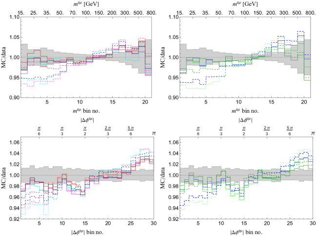
Figure 2: The dashed colored lines show six different SM predictions (MC) normalized to data given in Ref. Aad et al. (2023). The solid lines include the NP contribution from our benchmark model obtained by a combined global fit to $m^{e\mu}$ and $\Delta\phi^{e\mu}$ data. The black lines are obtained by averaging the six predictions and the grey band shows the total uncertainty (systematic and statistical). One can see that the agreement between theory and experiment is significantly increased by adding a NP effect.

In the next section, we will study the ATLAS analysis with six different MC predictions provided by ATLAS and set up our framework for the NP fit. We will then consider our benchmark scenario for the simplified model $pp\to H\to SS^{\prime}\to WWb\bar{b}$, with $m_{S}=152\,$GeV and $m_{S^{\prime}}=95\,$GeV in Sec. III and conclude in Sec. IV.

II Data and Fit

The latest ATLAS analysis of differential $t\bar{t}$ cross-section Aad et al. (2023) presents several distributions for the leptons, including the invariant mass of the electron-muon pair ($m^{e\mu}$), the sum of the energies $E^{e}+E^{\mu}$, the angle between the leptons ($|\Delta\phi^{e\mu}|$), the sum of transverse momentum of the leptons ($p_{T}^{e}+p_{T}^{\mu}$) and the pseudo-rapidity of the lepton system ($\eta$). Here, we will focus on $m^{e\mu}$ and $|\Delta\phi^{e\mu}|$, as they have a fine binning and show the most significant deviations from the SM predictions. However, we will later predict the other different distributions to show the consistency of the NP explanation.

The main input for our analysis is thus Fig. 10 and 11 in Ref. Aad et al. (2023), showing the ratio of expected events within the SM (MC) over measured events (data) per bin $i$, ${\rm MC}|_{i}/{\rm data}|_{i}=x_{i}$, as well as the corresponding Tables 21 and 24 where the normalized cross sections and the (relative) systematic and statistical uncertainties for each bin ($\delta_{i}$) are given. Note that ATLAS normalized the differential cross-section to the total one such that the resulting $\chi^{2}$ value is minimized. In particular, $m^{e\mu}$ is given in 21 bins between {0.0, 15.0, 20.0, 25.0, 30.0, 35.0, 40.0, 50.0, 60.0, 70.0, 85.0, 100.0, 120.0, 150.0, 175.0, 200.0, 250.0, 300.0, 400.0, 500.0, 650.0, 800.0} GeV. As the binning for low values of $m_{e\mu}$ is relatively thin, we display the data in Fig. 2 with equal size for all bins to give also optically equal weight to each of them. For $|\Delta\phi^{e\mu}|$ each bin corresponds to an angle of $\pi/30$ and we therefore have 30 bins.

In order to obtain the SM prediction for each bin (and thus $x_{i}$) for the different distributions, ATLAS generated $t\bar{t}$ samples with several different matrix element generators, parton shower, and fragmentation simulations. In particular, the nominal sample was obtained using Powheg Box Frixione et al. (2007a); Alioli et al. (2010); Frixione et al. (2007b) with NNPDF3.0 PDF Ball et al. (2015) interfaced with Pythia 8.230 Sjostrand et al. (2006); Sjöstrand et al. (2015). Alternative simulations used MADGRAPH_AMC$@$NLO Alwall et al. (2014) (aMC$@$NLO) with NNPDF2.3 PDF Ball et al. (2013) for the event generation or Powheg Box interfaced with Herwig 7.0.4 Bahr et al. (2008); Bellm et al. (2016) or 7.1.3 Bellm et al. (2017). In the relevant plots the following six different options are shown (using the same colour coding as in Ref. Aad et al. (2023)):

• aMC$@$NLO+Herwig7.1.3

• Powheg+Herwig7.0.4

• Powheg+Pythia8

• Powheg+Herwig7.1.3

• aMC$@$NLO+Pythia8

• Powheg+Pythia8 (rew.)

In the last case, the $p_{T}$ of the top quark was reweighted using the kinematics of the top quarks after initial- and final-state radiation using next-to-next-to-leading order QCD with next-to-leading EW corrections Czakon et al. (2017). The values of $x_{i}$, are unfortunately not yet available in numerical form and we thus obtained them by digitizing the lower panels of Fig. 10 and 11 using WebPlotDigitizer v4.6 Rohatgi (2022) with the integrated automatic tool. The results of this extraction for $m^{e\mu}$ and $|\Delta\phi^{e\mu}|$ are shown in Fig. 2 as dashed lines.

rowsep=0.1cm

	${m^{e\mu}}$				$\Delta{\phi^{e\mu}}$				${m^{e\mu}}+\Delta{\phi^{e\mu}}$
	$\chi_{{\rm{SM}}}^{2}$	$\chi_{{\rm{NP}}}^{2}$	$\sigma_{{\rm{NP}}}$	Sig.	$\chi_{{\rm{SM}}}^{2}$	$\chi_{{\rm{NP}}}^{2}$	$\sigma_{{\rm{NP}}}$	Sig.	$\chi_{{\rm{SM}}}^{2}$	$\chi_{{\rm{NP}}}^{2}$	$\sigma_{{\rm{NP}}}$	Sig.	$m_{S}$[GeV]
Powheg+Pyhtia8	146	50	10pb	9.8$\sigma$	183	73	11pb	10.5$\sigma$	213	102	9pb	10.5$\sigma$	$143-156$
aMC@NLO+Herwig7.1.3	31	13	4pb	4.2$\sigma$	96	38	8pb	7.6$\sigma$	102	68	5pb	5.8$\sigma$	$--$
aMC@NLO+Pythia8	89	14	9pb	8.7$\sigma$	277	83	15pb	14.0$\sigma$	291	163	10pb	11.3$\sigma$	148-157
Powheg+Herwig7.1.3	138	32	10pb	10.3$\sigma$	245	93	13pb	12.3$\sigma$	261	126	10pb	11.6$\sigma$	149-156
Powheg+Pythia8 (rew)	40	12	5pb	5.3$\sigma$	54	26	6pb	5.3$\sigma$	69	35	5pb	5.8$\sigma$	$--$
Powheg+Herwig7.0.4	186	41	12pb	12.0$\sigma$	263	99	14pb	12.8$\sigma$	294	126	12pb	13.0$\sigma$	149-156
Average	93	23	8pb	8.4$\sigma$	172	63	11pb	10.4$\sigma$	182	88	9pb	9.6$\sigma$	143-157

Table 1: $\chi^{2}$ values, preferred cross section ($\sigma_{\rm NP}$) sigifcance (Sig.) etc. for the individual $m^{e\mu}$ and $|\Delta\phi^{e\mu}|$ distributions and the combined fit to them for the six different SM simulations and their average. The $\chi^{2}_{\rm NP}$ is for our benchmark scenario with $m_{S}\approx 152\,$GeV while the $m_{S}$ gives the preferred rage of it from the fit, assuming it to be a free parameter. A dash in the $m_{S}$ column means that the preferred $1\sigma$ rage is wider than $140\,$GeV–$160\,$GeV. Note that the cross section preferred by $m^{e\mu}$ and $|\Delta\phi^{e\mu}|$ individually are in very good agreement with each other. The preferred NP cross-section $\sigma_{\rm NP}$ is given for Br$S^{\prime}\to b\bar{b}\approx 100\%$ and Br$S\to WW\approx 100\%$.

There are two main sources of correlations. First, there is the correlation between events in $m^{e\mu}$ bins and in $|\Delta\phi^{e\mu}|$ bins since they are overlapping (i.e. not mutually exclusive). To estimate this, we simulated 1600k events of $pp\to t\bar{t}$ in the SM with MadGraph5aMC@NLO Alwall et al. (2014), Pythia8.3 Sjöstrand et al. (2015), and Delphes de Favereau et al. (2014). Let $N_{i}^{m}$ ($N_{\alpha}^{\Delta\phi}$) be the number of events in the bin $i^{\rm th}$ ($\alpha^{\rm th}$) of $m^{e\mu}$ ($\Delta\phi^{e\mu}$), disregarding the $\Delta\phi^{e\mu}$ ($m^{e\mu}$) values. $N_{i\alpha}$ denotes the number of events that are both within $i^{\rm th}$ bin of $m^{e\mu}$ and the $\alpha^{\rm th}$ bin of $\Delta\phi^{e\mu}$. The correlation matrix between $m^{e\mu}$ and $\Delta\phi^{e\mu}$ is then given by

$${\rho_{i\alpha}}=\frac{{{N_{i\alpha}}}}{{\sqrt{\sum\limits_{j}{N_{j}^{m}}}\sqrt{\sum\limits_{\beta}{N_{\beta}^{\phi}}}}}\,.$$ (1)

The second source leading to a correlation is due to the normalization of the distributions to the total cross-section. Within a single distribution ($m^{e\mu}$ or $\Delta\phi^{e\mu}$), one has

$${\rho_{ij}}={\delta_{ij}}-\frac{{2{N_{i}}{N_{j}}}}{{N^{2}}}\,,$$ (2)

i.e. an anti-correlation. With this at hand, we can calculate the $\chi^{2}$ for the different SM predictions given by ATLAS, see Table 1, in the standard way.

Next, we can inject an arbitrary NP signal which we normalize to the corresponding total NP cross-section as well as the (normalized) SM cross-section. This means for each (normalized) value of bin $i$ of a given distribution we add a normalized cross-section of

$$r_{i}=\frac{\sigma_{i}^{\rm NP}/\sigma^{\rm NP}}{\sigma_{i}^{\rm SM}/\sigma^{\rm SM}}\,,$$ (3)

with $\sum_{i}\sigma_{i}^{\rm NP,SM}=\sigma^{\rm NP,SM}$. We can now calculate the $\chi^{2}$ including the NP contribution. Treating NP linearly as a small perturbation we have

$$\chi_{{\rm{NP}}}^{2}=\sum\limits_{i,j=1}{\frac{{\left({a{x_{i}}+{\varepsilon_{{\rm{NP}}}}{r_{i}}-1}\right){\rho_{ij}}\left({a{x_{j}}+{\varepsilon_{{\rm{NP}}}}{r_{j}}-1}\right)}}{{\delta_{i}\delta_{j}}}}.$$ (4)

In order to find the best fit, the $\chi^{2}$ function is minimized with respect to $\epsilon_{\rm NP}$ and $a$, the latter taking into account the possible rescaling of the total cross-section (as done in the ATLAS analysis). Importantly, this means that even if the NP contribution is localized at low $m^{e\mu}$ or $|\Delta\phi^{e\mu}|$ values, higher values are affected since the (predicted) values of $x_{i}$ are lowered for a non-vanishing NP effect. The values of $r_{i}$ must now be determined from a NP and SM simulation and the total NP cross-section can be approximated by

$$\sigma_{\rm NP}\approx\varepsilon_{{\rm{NP}}}\sum_{i}r_{i}\sigma^{\rm EXP}_{i}\,,$$ (5)

if the NP is a small correction to the SM.

III Benchmark Model

Let us now consider a simplified model in which $H$ is produced via gluon fusion and decays into two lighter scalars $S$ and $S^{\prime}$. We use the hints for di-photon resonances to fix $m_{S}=152\,$GeV (for now) and $m_{S^{\prime}}=95\,$GeV and assume $m_{H}>m_{S}+m_{S\prime}$ such that an on-shell decay is possible. For concreteness, we will fix $m_{H}=270\,$GeV but we checked that varying its mass has a negligible impact on the fit. Furthermore, we will assume that the dominant decay of $S$ is into pairs of $W$ bosons while $S^{\prime}$ decays dominantly to $b\bar{b}$. Note that this is naturally the case if $S$ is a SM-like Higgs and $S^{\prime}$ is the neutral component of an $SU(2)_{L}$ triplet with hypercharge 0.

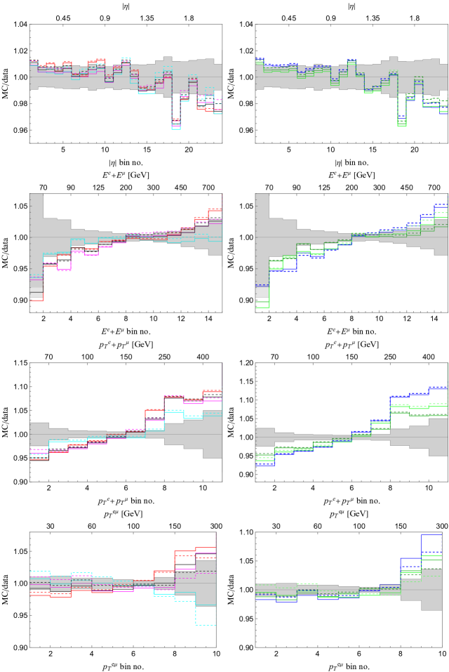
Figure 4: SM values (dashed) and NP predictions (solid), using the best fit from $m^{e\mu}$ and $|\Delta\phi^{e\mu}|$, for six other differential distributions given in the ATLAS paper and their average (black). One can see that while NP improves the agreement of theory with data, the effect is not as significant as in $m^{e\mu}$ and $|\Delta\phi^{e\mu}|$, justifying our input choice. Only $y^{e\mu}$ and $p_{T}^{e\mu}$ are not shown since here both the tensions within the SM as well as the NP effect are very small.

We simulated in this setup the process $pp\to H\to SS^{\prime}\to(WW^{(*)}\to\ell^{+}\nu\ell^{-}\nu)b\bar{b}$, with $\ell=e,\mu,\tau$, and the tau lepton subsequently decaying, using MadGraph5aMC@NLO Alwall et al. (2014), Pythia8.3 Sjöstrand et al. (2015), and Delphes de Favereau et al. (2014). Note that since our NP contribution is a small perturbation compared to the SM cross-section, the dependence on the MC generators used is small. This now determines the shape of the NP contribution to the differential lepton distributions. As outlined in the introduction, we will focus on $m^{e\mu}$ and $|\Delta\phi^{e\mu}|$, including the correlations among them as described in the previous section. The results are shown as solid lines in Fig. 2. One can see that for all SM simulations used by ATLAS, the agreement with data is significantly improved. In fact, as given in Table. 1, the $\chi^{2}$ is reduced between $\Delta\chi^{2}=34$ and $\Delta\chi^{2}=158$, corresponding to a preference of the NP model over the SM hypothesis by $5.8\sigma$–$13.0\sigma$ while the average of the SM predictions results in $9.6\sigma$. In the appendix, we use the best-fit points for the various SM predictions and their combination to predict the differential distributions. We find in Fig. 4 that while also here the agreement with data is improved, the effect (reduction of the $\chi^{2}$) is much less significant than for $m^{e\mu}$ and $|\Delta\phi^{e\mu}|$, justifying our choice of input for the global fit.

So far, we fixed the masses of $S$ and $S^{\prime}$ by using the hints for narrow di-photon resonances and took $m_{H}=270\,$GeV as a benchmark point which avoids constraints from SUSY and non-resonant di-Higgs searches. Let us now discuss the dependence on the masses. First of all, we checked that the effect of changing either the mass of $H$ or of ${S^{\prime}}$ is very small. This means that one can pick any value for $m_{H}$ so that this does not need to be counted as a degree of freedom in the statistical analysis. Now we can find the best-fit value in the $m_{S}$-$\epsilon_{\rm NP}$ plane by averaging the $x_{i}$ values of the six different MC simulations. For this, we generated 500k events each for $m_{S}$ between 140 GeV and 160 GeV in 2 GeV steps and interpolated. As one can see from Fig. 3 the result is perfectly consistent with a mass of $152\,$GeV as suggested by the invariant mass of the di-photon system Aad et al. (2021).

Finally, let us consider the consistency of the preferred signal strength for $pp\to H\to SS^{\prime}$ with the di-photon excess at 95 GeV. The branching ratio to photons of an SM-like Higgs with $95\,$GeV is $\approx\!1.4\times 10^{-3}$, Br$[S^{\prime}\to b\bar{b}]\approx\!0.86$ de Florian et al. (2016); Braaten and Leveille (1980); Sakai (1980); Inami and Kubota (1981); Gorishnii et al. (1984, 1991a, 1990, 1991b); Djouadi et al. (1998); Degrassi and Maltoni (2005); Passarino et al. (2007); Actis et al. (2009); Djouadi et al. (1991); Chetyrkin (1997); Baikov et al. (2006); Spira et al. (1992) and the production cross section at $13\,$TeV via gluon fusion is $\approx\!68$pb de Florian et al. (2016); Graudenz et al. (1993); Spira et al. (1995); Anastasiou and Melnikov (2002); Harlander and Kilgore (2002, 2001); Aglietti et al. (2007); Li et al. (2016); Anastasiou et al. (2007); Harlander and Kant (2005); Ravindran et al. (2003). Given that the preferred $\gamma\gamma$ signal at $95\,$GeV, with respect to a (hypothetical) SM-like Higgs with a mass of $95\,$GeV, is $\mu_{\gamma\gamma}=0.24^{+0.09}_{-0.08}$ Biekötter et al. (2023) we can see in Fig. 3 that, under the assumption that $S^{\prime}$ is SM-like and Br$[S\to WW^{*}]\approx 100\%$, the associated production of $S^{\prime}$, determined by the preferred signal strength from $t\bar{t}$, perfectly explains the excess.

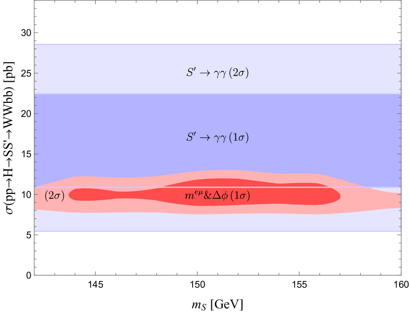
Figure 3: Preferred regions from the $t\bar{t}$ differential distributions (red) as a function of $m_{S}$ and the total cross section $pp\to H\to SS^{\prime}\to WWbb$ assuming $S^{\prime}$ to be SM-like and Br$[S\to WW]=100\%$. The blue region is preferred by the $95\,$GeV $\gamma\gamma$ signal strength.

IV Conclusions

ATLAS found that the measured differential lepton distributions in its $t\bar{t}$ analysis significantly deviate from the SM predictions obtained for different combinations of simulators: “No model (simulation) can describe all measured distributions within their uncertainties.” Taking into account the performance of the ATLAS detector w.r.t. leptons and the level of sophistication of the SM simulations, this suggests that the measurement is contaminated by NP contributions.

In this article, we propose that the process $pp\to H\to SS^{\prime}\to WWb\bar{b}$ constitutes a NP background to the measurements of $t\bar{t}$ differential lepton distributions. Motivated by the hints for di-photon resonances $\approx\!95\,$GeV and $\approx\!152$GeV we considered the benchmark point with $S^{\prime}$ and $S$ having the corresponding masses and decaying to $b\bar{b}$ and $WW$, respectively (with $m_{H}=270\,$GeV). We find that this NP hypothesis is preferred over the SM one by $5.8\sigma$ to $13\sigma$, depending on which of the six SM simulations employed by ATLAS is considered. In fact, all differential distributions, in particular $m^{e\mu}$ and $|\Delta\phi^{e\mu}|$, are well described once NP is included and averaging the SM predictions a significance of $9.6\sigma$ is found (see Table 1).

Varying $m_{S}$, to which the distributions are most sensitive among the new scalar masses, we showed that the preferred range is compatible with $m_{S}\approx 152\,$GeV, as motivated by the $\gamma\gamma$ and $WW$ excesses. Since the latter analysis employs a jet veto, this further disfavours the possibility of that higher order QCD corrections of the tension in the $t\bar{t}$ differential distributions. Furthermore, averaging the six different SM predictions $\sigma(pp\to H\to SS^{\prime}\to WWb\bar{b})\approx 9$pb is preferred by $t\bar{t}$ data. Assuming that $S^{\prime}$ is SM-like, this results in a di-photon signal strength in agreement with the $\gamma\gamma$ excess. This provides further support for the emerging excess at $\approx\,$95 GeV which naturally has a large $b\bar{b}$ branching ratio and opens a window of opportunity to further explore this boson in associated production. Finally, since for $S$ a dominant decay to $W$ bosons is needed while the $ZZ$ rate should be low to respect the limits from inclusive $4\ell$ searches. This suggests that it could be the neutral component of the $SU(2)_{L}$ triplet with hypercharge 0, as also motivated by the $W$-mass average.

References

- Zyla et al. (2020) P. A. Zyla et al. (Particle Data Group), PTEP 2020, 083C01 (2020).
- Higgs (1964a) P. W. Higgs, Phys. Lett. 12, 132 (1964a).
- Englert and Brout (1964) F. Englert and R. Brout, Phys. Rev. Lett. 13, 321 (1964).
- Higgs (1964b) P. W. Higgs, Phys. Rev. Lett. 13, 508 (1964b).
- Guralnik et al. (1964) G. S. Guralnik, C. R. Hagen, and T. W. B. Kibble, Phys. Rev. Lett. 13, 585 (1964).
- Aad et al. (2012) G. Aad et al. (ATLAS), Phys. Lett. B 716, 1 (2012), arXiv:1207.7214 [hep-ex] .
- Chatrchyan et al. (2012a) S. Chatrchyan et al. (CMS), Phys. Lett. B 716, 30 (2012a), arXiv:1207.7235 [hep-ex] .
- Langford (2021) J. M. Langford (ATLAS, CMS), PoS LHCP2020, 136 (2021).
- ATL (2021) (2021).
- Schael et al. (2013) S. Schael et al. (ALEPH, DELPHI, L3, OPAL, LEP Electroweak), Phys. Rept. 532, 119 (2013), arXiv:1302.3415 [hep-ex] .
- Aaij et al. (2022) R. Aaij et al. (LHCb), JHEP 01, 036 (2022), arXiv:2109.01113 [hep-ex] .
- Aaltonen et al. (2022) T. Aaltonen et al. (CDF), Science 376, 170 (2022).
- ATL (2023) (2023).
- de Blas et al. (2022) J. de Blas, M. Pierini, L. Reina, and L. Silvestrini, Phys. Rev. Lett. 129, 271801 (2022), arXiv:2204.04204 [hep-ph] .
- Strumia (2022) A. Strumia, JHEP 08, 248 (2022), arXiv:2204.04191 [hep-ph] .
- Konetschny and Kummer (1977) W. Konetschny and W. Kummer, Phys. Lett. B 70, 433 (1977).
- Cheng and Li (1980) T. P. Cheng and L.-F. Li, Phys. Rev. D 22, 2860 (1980).
- Lazarides et al. (1981) G. Lazarides, Q. Shafi, and C. Wetterich, Nucl. Phys. B 181, 287 (1981).
- Schechter and Valle (1980) J. Schechter and J. W. F. Valle, Phys. Rev. D 22, 2227 (1980).
- Magg and Wetterich (1980) M. Magg and C. Wetterich, Phys. Lett. B 94, 61 (1980).
- Mohapatra and Senjanovic (1981) R. N. Mohapatra and G. Senjanovic, Phys. Rev. D 23, 165 (1981).
- Fileviez Perez et al. (2022) P. Fileviez Perez, H. H. Patel, and A. D. Plascencia, Phys. Lett. B 833, 137371 (2022), arXiv:2204.07144 [hep-ph] .
- Cheng et al. (2023) Y. Cheng, X.-G. He, F. Huang, J. Sun, and Z.-P. Xing, Nucl. Phys. B 989, 116118 (2023), arXiv:2208.06760 [hep-ph] .
- Chen et al. (2022) T.-K. Chen, C.-W. Chiang, and K. Yagyu, Phys. Rev. D 106, 055035 (2022), arXiv:2204.12898 [hep-ph] .
- Rizzo (2022) T. G. Rizzo, Phys. Rev. D 106, 035024 (2022), arXiv:2206.09814 [hep-ph] .
- Chao et al. (2022) W. Chao, M. Jin, H.-J. Li, and Y.-Q. Peng, (2022), arXiv:2210.13233 [hep-ph] .
- Wang et al. (2022) J.-W. Wang, X.-J. Bi, P.-F. Yin, and Z.-H. Yu, Phys. Rev. D 106, 055001 (2022), arXiv:2205.00783 [hep-ph] .
- Shimizu and Takeshita (2023) Y. Shimizu and S. Takeshita, Nucl. Phys. B 994, 116290 (2023), arXiv:2303.11070 [hep-ph] .
- Lazarides et al. (2022) G. Lazarides, R. Maji, R. Roshan, and Q. Shafi, Phys. Rev. D 106, 055009 (2022), arXiv:2205.04824 [hep-ph] .
- Senjanović and Zantedeschi (2023) G. Senjanović and M. Zantedeschi, Phys. Lett. B 837, 137653 (2023), arXiv:2205.05022 [hep-ph] .
- Crivellin et al. (2023) A. Crivellin, M. Kirk, and A. Thapa, (2023), arXiv:2305.03081 [hep-ph] .
- Chen et al. (2023) T.-K. Chen, C.-W. Chiang, and K. Yagyu, JHEP 06, 069 (2023), [Erratum: JHEP 07, 169 (2023)], arXiv:2303.09294 [hep-ph] .
- Ashanujjaman et al. (2023) S. Ashanujjaman, S. Banik, G. Coloretti, A. Crivellin, B. Mellado, and A.-T. Mulaudzi, (2023), arXiv:2306.15722 [hep-ph] .
- Barate et al. (2003) R. Barate et al. (LEP Working Group for Higgs boson searches, ALEPH, DELPHI, L3, OPAL), Phys. Lett. B 565, 61 (2003), arXiv:hep-ex/0306033 .
- Sirunyan et al. (2019a) A. M. Sirunyan et al. (CMS), Phys. Lett. B 793, 320 (2019a), arXiv:1811.08459 [hep-ex] .
- CMS (2022a) (2022a).
- CMS (2022b) (2022b).
- Aad et al. (2021) G. Aad et al. (ATLAS), JHEP 10, 013 (2021), arXiv:2104.13240 [hep-ex] .
- Bhattacharya et al. (2023) S. Bhattacharya, G. Coloretti, A. Crivellin, S.-E. Dahbi, Y. Fang, M. Kumar, and B. Mellado, (2023), arXiv:2306.17209 [hep-ph] .
- Buddenbrock et al. (2019) S. Buddenbrock, A. S. Cornell, Y. Fang, A. Fadol Mohammed, M. Kumar, B. Mellado, and K. G. Tomiwa, JHEP 10, 157 (2019), arXiv:1901.05300 [hep-ph] .
- von Buddenbrock et al. (2020) S. von Buddenbrock, R. Ruiz, and B. Mellado, Phys. Lett. B 811, 135964 (2020), arXiv:2009.00032 [hep-ph] .
- Hernandez et al. (2021) Y. Hernandez, M. Kumar, A. S. Cornell, S.-E. Dahbi, Y. Fang, B. Lieberman, B. Mellado, K. Monnakgotla, X. Ruan, and S. Xin, Eur. Phys. J. C 81, 365 (2021), arXiv:1912.00699 [hep-ph] .
- Fischer et al. (2022) O. Fischer et al., Eur. Phys. J. C 82, 665 (2022), arXiv:2109.06065 [hep-ph] .
- von Buddenbrock et al. (2018) S. von Buddenbrock, A. S. Cornell, A. Fadol, M. Kumar, B. Mellado, and X. Ruan, J. Phys. G 45, 115003 (2018), arXiv:1711.07874 [hep-ph] .
- Coloretti et al. (2023) G. Coloretti, A. Crivellin, S. Bhattacharya, and B. Mellado, (2023), arXiv:2302.07276 [hep-ph] .
- Aad et al. (2023) G. Aad et al. (ATLAS), JHEP 07, 141 (2023), arXiv:2303.15340 [hep-ex] .
- Beneke et al. (2012) M. Beneke, P. Falgari, S. Klein, and C. Schwinn, Nucl. Phys. B 855, 695 (2012), arXiv:1109.1536 [hep-ph] .
- Bärnreuther et al. (2012) P. Bärnreuther, M. Czakon, and A. Mitov, Phys. Rev. Lett. 109, 132001 (2012), arXiv:1204.5201 [hep-ph] .
- Czakon and Mitov (2012) M. Czakon and A. Mitov, JHEP 12, 054 (2012), arXiv:1207.0236 [hep-ph] .
- Botje et al. (2011) M. Botje et al., (2011), arXiv:1101.0538 [hep-ph] .
- Martin et al. (2009) A. D. Martin, W. J. Stirling, R. S. Thorne, and G. Watt, Eur. Phys. J. C 63, 189 (2009), arXiv:0901.0002 [hep-ph] .
- Ball et al. (2013) R. D. Ball et al., Nucl. Phys. B 867, 244 (2013), arXiv:1207.1303 [hep-ph] .
- Gao et al. (2014) J. Gao, M. Guzzi, J. Huston, H.-L. Lai, Z. Li, P. Nadolsky, J. Pumplin, D. Stump, and C. P. Yuan, Phys. Rev. D 89, 033009 (2014), arXiv:1302.6246 [hep-ph] .
- Lai et al. (2010) H.-L. Lai, M. Guzzi, J. Huston, Z. Li, P. M. Nadolsky, J. Pumplin, and C. P. Yuan, Phys. Rev. D 82, 074024 (2010), arXiv:1007.2241 [hep-ph] .
- Aaboud et al. (2017) M. Aaboud et al. (ATLAS), Eur. Phys. J. C 77, 804 (2017), arXiv:1709.09407 [hep-ex] .
- Aad et al. (2020) G. Aad et al. (ATLAS), Eur. Phys. J. C 80, 528 (2020), arXiv:1910.08819 [hep-ex] .
- Sirunyan et al. (2019b) A. M. Sirunyan et al. (CMS), JHEP 02, 149 (2019b), arXiv:1811.06625 [hep-ex] .
- Sirunyan et al. (2020a) A. M. Sirunyan et al. (CMS), Eur. Phys. J. C 80, 658 (2020a), arXiv:1904.05237 [hep-ex] .
- Sirunyan et al. (2020b) A. M. Sirunyan et al. (CMS), Phys. Rev. D 102, 092013 (2020b), arXiv:2009.07123 [hep-ex] .
- Sirunyan et al. (2018) A. M. Sirunyan et al. (CMS), JHEP 10, 117 (2018), arXiv:1805.07399 [hep-ex] .
- Aad et al. (2010) G. Aad et al. (ATLAS), Eur. Phys. J. C 70, 823 (2010), arXiv:1005.4568 [physics.ins-det] .
- Sirunyan et al. (2020c) A. M. Sirunyan et al. (CMS), Eur. Phys. J. C 80, 4 (2020c), arXiv:1903.12179 [hep-ex] .
- Aad et al. (2019) G. Aad et al. (ATLAS), JINST 14, P12006 (2019), arXiv:1908.00005 [hep-ex] .
- Aaboud et al. (2018) M. Aaboud et al. (ATLAS), Eur. Phys. J. C 78, 903 (2018), arXiv:1802.08168 [hep-ex] .
- Khachatryan et al. (2015) V. Khachatryan et al. (CMS), JINST 10, P06005 (2015), arXiv:1502.02701 [physics.ins-det] .
- Chatrchyan et al. (2012b) S. Chatrchyan et al. (CMS), JINST 7, P10002 (2012b), arXiv:1206.4071 [physics.ins-det] .
- Tumasyan et al. (2023) A. Tumasyan et al. (CMS), Eur. Phys. J. C 83, 667 (2023), arXiv:2206.09466 [hep-ex] .
- ATL (2022) (2022), arXiv:2207.00338 [hep-ex] .
- Ježo et al. (2023) T. Ježo, J. M. Lindert, and S. Pozzorini, (2023), arXiv:2307.15653 [hep-ph] .
- Frixione et al. (2007a) S. Frixione, P. Nason, and C. Oleari, JHEP 11, 070 (2007a), arXiv:0709.2092 [hep-ph] .
- Alioli et al. (2010) S. Alioli, P. Nason, C. Oleari, and E. Re, JHEP 06, 043 (2010), arXiv:1002.2581 [hep-ph] .
- Frixione et al. (2007b) S. Frixione, P. Nason, and G. Ridolfi, JHEP 09, 126 (2007b), arXiv:0707.3088 [hep-ph] .
- Ball et al. (2015) R. D. Ball et al. (NNPDF), JHEP 04, 040 (2015), arXiv:1410.8849 [hep-ph] .
- Sjostrand et al. (2006) T. Sjostrand, S. Mrenna, and P. Z. Skands, JHEP 05, 026 (2006), arXiv:hep-ph/0603175 .
- Sjöstrand et al. (2015) T. Sjöstrand, S. Ask, J. R. Christiansen, R. Corke, N. Desai, P. Ilten, S. Mrenna, S. Prestel, C. O. Rasmussen, and P. Z. Skands, Comput. Phys. Commun. 191, 159 (2015), arXiv:1410.3012 [hep-ph] .
- Alwall et al. (2014) J. Alwall, R. Frederix, S. Frixione, V. Hirschi, F. Maltoni, O. Mattelaer, H. S. Shao, T. Stelzer, P. Torrielli, and M. Zaro, JHEP 07, 079 (2014), arXiv:1405.0301 [hep-ph] .
- Bahr et al. (2008) M. Bahr et al., Eur. Phys. J. C 58, 639 (2008), arXiv:0803.0883 [hep-ph] .
- Bellm et al. (2016) J. Bellm et al., Eur. Phys. J. C 76, 196 (2016), arXiv:1512.01178 [hep-ph] .
- Bellm et al. (2017) J. Bellm et al., (2017), arXiv:1705.06919 [hep-ph] .
- Czakon et al. (2017) M. Czakon, D. Heymes, A. Mitov, D. Pagani, I. Tsinikos, and M. Zaro, JHEP 10, 186 (2017), arXiv:1705.04105 [hep-ph] .
- Rohatgi (2022) A. Rohatgi, “Webplotdigitizer: Version 4.6,” (2022).
- de Favereau et al. (2014) J. de Favereau, C. Delaere, P. Demin, A. Giammanco, V. Lemaître, A. Mertens, and M. Selvaggi (DELPHES 3), JHEP 02, 057 (2014), arXiv:1307.6346 [hep-ex] .
- de Florian et al. (2016) D. de Florian et al. (LHC Higgs Cross Section Working Group), 2/2017 (2016), 10.23731/CYRM-2017-002, arXiv:1610.07922 [hep-ph] .
- Braaten and Leveille (1980) E. Braaten and J. P. Leveille, Phys. Rev. D 22, 715 (1980).
- Sakai (1980) N. Sakai, Phys. Rev. D 22, 2220 (1980).
- Inami and Kubota (1981) T. Inami and T. Kubota, Nucl. Phys. B 179, 171 (1981).
- Gorishnii et al. (1984) S. G. Gorishnii, A. L. Kataev, and S. A. Larin, Sov. J. Nucl. Phys. 40, 329 (1984).
- Gorishnii et al. (1991a) S. G. Gorishnii, A. L. Kataev, S. A. Larin, and L. R. Surguladze, Phys. Lett. B 256, 81 (1991a).
- Gorishnii et al. (1990) S. G. Gorishnii, A. L. Kataev, S. A. Larin, and L. R. Surguladze, Mod. Phys. Lett. A 5, 2703 (1990).
- Gorishnii et al. (1991b) S. G. Gorishnii, A. L. Kataev, S. A. Larin, and L. R. Surguladze, Phys. Rev. D 43, 1633 (1991b).
- Djouadi et al. (1998) A. Djouadi, P. Gambino, and B. A. Kniehl, Nucl. Phys. B 523, 17 (1998), arXiv:hep-ph/9712330 .
- Degrassi and Maltoni (2005) G. Degrassi and F. Maltoni, Nucl. Phys. B 724, 183 (2005), arXiv:hep-ph/0504137 .
- Passarino et al. (2007) G. Passarino, C. Sturm, and S. Uccirati, Phys. Lett. B 655, 298 (2007), arXiv:0707.1401 [hep-ph] .
- Actis et al. (2009) S. Actis, G. Passarino, C. Sturm, and S. Uccirati, Nucl. Phys. B 811, 182 (2009), arXiv:0809.3667 [hep-ph] .
- Djouadi et al. (1991) A. Djouadi, M. Spira, J. J. van der Bij, and P. M. Zerwas, Phys. Lett. B 257, 187 (1991).
- Chetyrkin (1997) K. G. Chetyrkin, Phys. Lett. B 390, 309 (1997), arXiv:hep-ph/9608318 .
- Baikov et al. (2006) P. A. Baikov, K. G. Chetyrkin, and J. H. Kuhn, Phys. Rev. Lett. 96, 012003 (2006), arXiv:hep-ph/0511063 .
- Spira et al. (1992) M. Spira, A. Djouadi, and P. M. Zerwas, Phys. Lett. B 276, 350 (1992).
- Graudenz et al. (1993) D. Graudenz, M. Spira, and P. M. Zerwas, Phys. Rev. Lett. 70, 1372 (1993).
- Spira et al. (1995) M. Spira, A. Djouadi, D. Graudenz, and P. M. Zerwas, Nucl. Phys. B 453, 17 (1995), arXiv:hep-ph/9504378 .
- Anastasiou and Melnikov (2002) C. Anastasiou and K. Melnikov, Nucl. Phys. B 646, 220 (2002), arXiv:hep-ph/0207004 .
- Harlander and Kilgore (2002) R. V. Harlander and W. B. Kilgore, Phys. Rev. Lett. 88, 201801 (2002), arXiv:hep-ph/0201206 .
- Harlander and Kilgore (2001) R. V. Harlander and W. B. Kilgore, Phys. Rev. D 64, 013015 (2001), arXiv:hep-ph/0102241 .
- Aglietti et al. (2007) U. Aglietti, R. Bonciani, G. Degrassi, and A. Vicini, JHEP 01, 021 (2007), arXiv:hep-ph/0611266 .
- Li et al. (2016) H.-L. Li, P.-C. Lu, Z.-G. Si, and Y. Wang, Chin. Phys. C 40, 063102 (2016), arXiv:1508.06416 [hep-ph] .
- Anastasiou et al. (2007) C. Anastasiou, S. Beerli, S. Bucherer, A. Daleo, and Z. Kunszt, JHEP 01, 082 (2007), arXiv:hep-ph/0611236 .
- Harlander and Kant (2005) R. Harlander and P. Kant, JHEP 12, 015 (2005), arXiv:hep-ph/0509189 .
- Ravindran et al. (2003) V. Ravindran, J. Smith, and W. L. van Neerven, Nucl. Phys. B 665, 325 (2003), arXiv:hep-ph/0302135 .
- Biekötter et al. (2023) T. Biekötter, S. Heinemeyer, and G. Weiglein, (2023), arXiv:2306.03889 [hep-ph] .