Inductive Knowledge Graph Completion with GNNs and Rules: An Analysis

Abstract.

The task of inductive knowledge graph completion requires models to learn inference patterns from a training graph, which can then be used to make predictions on a disjoint test graph. Rule-based methods seem like a natural fit for this task, but in practice they significantly underperform state-of-the-art methods based on Graph Neural Networks (GNNs), such as NBFNet. We hypothesise that the underperformance of rule-based methods is due to two factors: (i) implausible entities are not ranked at all and (ii) only the most informative path is taken into account when determining the confidence in a given link prediction answer. To analyse the impact of these factors, we study a number of variants of a rule-based approach, which are specifically aimed at addressing the aforementioned issues. We find that the resulting models can achieve a performance which is close to that of NBFNet. Crucially, the considered variants only use a small fraction of the evidence that NBFNet relies on, which means that they largely keep the interpretability advantage of rule-based methods. Moreover, we show that a further variant, which does look at the full KG, consistently outperforms NBFNet.
Code is available at https://github.com/anilakash/IndKGC

1. Introduction

The aim of Knowledge Graph (KG) completion is to find plausible (entity,relation,entity) triples which are missing from a given KG. Standard KG completion models are best suited for densely connected static knowledge graphs. To encourage the study of KG completion methods that can be applied more widely, Teru et al. (2020) introduced the task of inductive KG completion (where the usual setting is then referred to as transductive). In the inductive setting, we have one knowledge graph for training and a separate knowledge graph for testing. Similar as for the transductive setting, the main evaluation task consists in answering link prediction queries of the form $(x,r,?)$, which require us to identify entities $y$ that make $(x,r,y)$ a valid triple. Crucially, in the inductive setting, the entities in the training and test KGs are different, so the model has to make predictions about entities that were not seen during training. Intuitively, we would thus expect that capturing inference patterns becomes crucial, which suggests that rule-based methods should be a natural fit for this setting. However, the literature on inductive KG completion is currently dominated by GNN models.

The aim of this paper is to analyse the reasons why rule-based methods underperform GNNs in inductive KG completion, and to suggest strategies for mitigating the underlying issues. We focus in particular on NBFNet (Zhu et al., 2021), as a state-of-the-art GNN model, and AnyBURL (Meilicke et al., 2019), as a state-of-the-art rule-based method. We start from the observation that standard rule-based methods have two key limitations, irrespective of the quality of the learned rules:

L1 (Zero-confidence entities):

For a link prediction query of the form $(x,r,?)$, rule-based methods only assign a non-zero confidence to entities that can be linked to $x$ by a rule. This means that the majority of entities will typically receive a confidence of 0. Rule-based methods thus make no attempt to rank entities which do not seem plausible.

L2 (Aggregation of evidence):

For most rule-based methods, the confidence in an answer candidate is essentially based on the confidence of a single rule. Intuitively, however, the more (ground) rules predict an answer candidate $y$, the more confident we should be in that candidate.

We analyse the effect of these issues by comparing the performance of AnyBURL and NBFNet with a hybrid approach. To address limitation L1, we simply rank the entities that receive a confidence of 0 with a different method, which is essentially used as a tie breaker. To facilitate the analysis, we use NBFNet for this purpose. By comparing the performance of this hybrid method with the standard AnyBURL set-up, we can evaluate the impact of ignoring zero-confidence entities on the overall performance.

To address L2, we essentially want to combine the confidence scores of all the ground rules that predict a given answer candidate. Doing this effectively is challenging, however, because we need to distinguish between cases where different rules provide independent evidence and cases where different variations of the same argument are found (Ott et al., 2021; Betz et al., 2022). To address this challenge, we experiment with a GNN-based strategy for aggregating the evidence provided by different rules. In particular, given a query $(x,r,?)$ and an answer candidate $y$, we determine all triples that appear in the ground rules that predict the triple $(x,r,y)$. We then consider the resulting sub-graph of the KG. We refer to this sub-graph as the rule instantiation graph. Essentially, rule instantiation graphs encode (i) which ground rules predict the triple $(x,r,y)$ and (ii) to what extent different rules depend on the same triples. We then use a GNN to predict the confidence in a triple $(x,r,y)$ from the corresponding rule instantiation graph. Since rule instantiation graphs are small, the proposed strategy largely keeps the interpretability advantage of rule-based methods, as we can easily inspect the full evidence that was taken into account for making a given prediction. Moreover, the focused nature of rule instantiation graphs also makes it less likely that the GNN will learn spurious correlations.

By combining the strategies for addressing L1 and L2, we achieve results which are close to those of NBFNet. As a final variant, we use NBFNet to re-rank the entities predicted by AnyBURL. When also using NBFNet for re-ranking the zero-confidence entities, we end up with a hybrid strategy which consistently outperforms the standard NBFNet, although without the interpretability advantage of rule-based methods. Note that in the this variant, AnyBURL is only used to partition to set of candidate answers into those with zero confidence and those that can be predicted by some rule. The fact that this variant outperforms NBFNet suggests that the latter is prone to learn spurious correlations.

Our main findings can be summarised as follows. (1) We confirm that the underperformance of AnyBURL indeed largely comes from limitations L1 and L2. (2) We introduce a new strategy for aggregating AnyBURL rules which consistently outperforms existing rule aggregation strategies. (3) We improve the state-of-the-art in inductive KG completion by using a simple hybrid strategy, in which AnyBURL is used to identify all the candidates with non-zero confidence, and NBFNet is then used for reranking these entities.

2. Related Work

In the last decade, several neural methods for transductive knowledge graph completion (KGC) have been proposed. Commonly used paradigms for KGC are GNN-based (Vashishth et al., 2020; Schlichtkrull et al., 2018), rule-based (Meilicke et al., 2019; Qu et al., 2021; Wu et al., 2022) and embedding-based approaches. Within the latter paradigm, various methods have been proposed, which differ among others in the considered embedding space, e.g. point-wise embeddings (Bordes et al., 2013; Lin et al., 2015; Zhang et al., 2020), complex embeddings (Trouillon et al., 2016; Sun et al., 2019; Zhang et al., 2019), or manifold embeddings (Balazevic et al., 2019; Chami et al., 2020). A shortcoming of these approaches is that, since they basically encode the connectivity patterns of specific entities, it is not straightforward to use them for newly emerging entities. Methods that rely on the textual descriptions of entities and relations (Yao et al., 2019; Liu et al., 2022; Markowitz et al., 2022) can overcome this limitation to some extent, but textual descriptions are not available in all domains, which limits their applicability.

Inductive Knowledge Graph Completion.

Most real-world KGs are dynamic, with new information being continuously added (e.g. new items or customers in recommendation systems). It is thus paramount to have methods that can make predictions about new entities, without relying on costly retraining. To be entity-agnostic, methods for inductive KGC have to capture the dependencies that hold between the different relations in the input KG. Inductive KGC methods currently fall into two main categories: rule-based methods and GNN-based methods. Classical rule learners, such as AnyBURL (Meilicke et al., 2019) and AMIE (Galárraga et al., 2015), explore paths in the KG to discover common patterns, and thus induce (weighted) Horn rules (Omran et al., 2018; Pirrò, 2020). Inspired by these classical methods, differentiable variants, approximating the search of rules, have recently also been studied (Yang et al., 2017; Sadeghian et al., 2019; Neelakantan et al., 2015; Das et al., 2017, 2018; Qu et al., 2021). On the other hand, GNNs have become a popular architecture for modelling the topological structure of graphs in different application domains (Hamilton, 2020). Indeed, the inherent capability of GNNs to describe subgraph patterns has led to the development of state-of-the-art GNN-based inductive KGC methods (Teru et al., 2020; Mai et al., 2021; Zhu et al., 2021; Liu et al., 2021; Yan et al., 2022; Zhang and Yao, 2022; Galkin et al., 2022). These methods vary in the way that graph information is used and generated. For example, GraIL (Teru et al., 2020) and CoMPILE (Mai et al., 2021) explicitly encode the subgraph enclosing the pair of nodes in a triple to predict whether that triple is plausible. Such methods are very expensive as a different subgraph has to be generated for each answer candidate, which is not feasible in large KGs. By contrast, NBFNet (Zhu et al., 2021) and RED-GNN (Zhang and Yao, 2022) dynamically generate the set of relational paths between the entity from the query and the different candidate answers. Variants of NBFNet which only expand the most promising paths between two nodes have also been investigated (Zhu et al., 2022; Zhang et al., 2022). The CBGNN model (Zhang and Yao, 2022) uses GNNs to learn the representation of cycles, which is inspired by the close connection between cycles and rules. RefactorGNN (Chen et al., 2022) is a GNN-based model for inductive KG completion, which is designed to mimic the gradient descent training dynamic of transductive methods such as DistMult. (Yang et al., 2015). As an alternative to GNNs, NodePiece (Galkin et al., 2022) uses transformers to learn entity representations from a fixed-size vocabulary of tokens, which can refer to anchor nodes in a graph or relation types.

To the best of our knowledge, this paper is the first attempt to analyse the performance of rule-based methods for inductive KGC, and to develop strategies to integrate them with GNNs. The closest to our paper is the work by Meilicke et al. (2021), which analyses the performance of AnyBURL in the transductive setting and introduces a hybrid method that combines AnyBURL with KG embeddings.

3. Background

In this section, we recall the inductive KG completion setting (Section 3.1), and provide some background on the two methods we will focus on: AnyBURL (Section 3.2) and NBFNet (Section 3.3).

3.1. Inductive KG Completion

We recall the inductive KG completion setting that was introduced by Teru et al. (2020). In this setting, we are given two knowledge graphs: $\mathcal{G}_{\textit{train}}$ and $\mathcal{G}_{\textit{test}}$. None of the entities from $\mathcal{G}_{\textit{test}}$ appears in $\mathcal{G}_{\textit{train}}$. However, we are guaranteed that every relation that appears in $\mathcal{G}_{\textit{test}}$ also appears in $\mathcal{G}_{\textit{train}}$. The aim is to learn the parameters $\theta$ of a link prediction model using $\mathcal{G}_{\textit{train}}$ only. Given a link prediction query $(x,r,?)$, this model assigns as score $f_{\theta}(y|x,r,\mathcal{G})$ to candidate answers $y$, reflecting its confidence that $(x,r,y)$ is a valid triple, given the information encoded in $\mathcal{G}$. To train the parameters of the model, for each triple $(x,r,y)\in\mathcal{G}_{\textit{train}}$, one or more corrupted triples $(x,r,y^{\prime})$ are generated, and the model is trained to score $f_{\theta}(y|x,r,\mathcal{G}_{\textit{train}}\setminus\{(x,r,y)\})$ higher than $f_{\theta}(y^{\prime}|x,r,\mathcal{G}_{\textit{train}}\setminus\{(x,r,y)\})$, which can be implemented using binary cross-entropy, among others. Once the parameters $\theta$ have been learned, the model is used for link prediction on $\mathcal{G}_{\textit{test}}$. To this end, 10% of the edges in $\mathcal{G}_{\textit{test}}$ are held out as test triples. Given a test triple $(x,r,y)$, the model is used to score all candidate answers against the query $(x,r,?)$. These scores are then used to rank the candidates. The same process is also used for queries of the form $(?,r,y)$.

In the experiments reported in (Teru et al., 2020), the set of candidate answers consisted of the answer $y$, along with 50 randomly chosen entities from $\mathcal{G}_{\textit{test}}$. This choice was made because of the limited scalability of their model. In line with standard practice for transductive KG completion, papers on inductive KG completion have recently started to report results for the more natural setting where every entity in $\mathcal{G}_{\textit{test}}$ is considered as a candidate answer (Zhang and Yao, 2022; Chen et al., 2022).

3.2. AnyBURL

AnyBURL (Meilicke et al., 2019) has been designed to work as a rule learner for KGs. First note that a triple $(x,r,y)$ can be seen as a first-order atom of the form $r(x,y)$. A ground path rule of length $n$ is a rule of the form $b_{1}(e_{1},e_{2})\wedge\dots\wedge b_{n}(e_{n},e_{n+1})\rightarrow h(e_{1},e_{n+1})$, where each $e_{i}$ is an entity from the KG. Note how the body of such a rule corresponds to a path in the knowledge graph. The rule expresses that when the triples $(e_{1},b_{1},e_{2}),\dots,(e_{n},b_{n},e_{n+1})$ all belong to the KG, we would expect the triple $(e_{1},h,e_{n+1})$ to be included as well. A closed path rule is a rule of the form $b_{1}(X_{1},X_{2})\wedge\dots\wedge b_{n}(X_{n},X_{n+1})\rightarrow h(X_{1},X_{n+1})$, where the arguments of each relation are now variables. The groundings of such a rule are all the ground path rules that can be obtained by replacing all variables with specific entities. The aim of AnyBURL is to learn a set of closed path rules, along with their confidence, which intuitively reflects how many of its groundings are satisfied in the given KG. Once the rules have been learned, they can be used for answering link prediction queries of the form $(x,r,?)$. The confidence of an answer candidate $y$ is given by the most confident rule which can predict the fact $r(x,y)$. Entities which are not predicted by any of the rules receive a confidence degree of 0. In principle, the answer candidates are ranked according to their confidence degree. However, when a tie between two entities $y_{1}$ and $y_{2}$ occurs, their relative position is decided by looking at the second-most confident rule that predicts $r(x,y_{1})$ and $r(x,y_{2})$, if any. This process can be repeated, by looking at more rules until the tie is broken.

A number of approaches have already been considered for improving AnyBURL by aggregating the confidence scores of different rules that predict the same triple. The most straightforward solution is noisy-or: if a fact is predicted by rules with confidence scores $c_{1},...,c_{n}$ then the overall confidence could be computed as $1-\prod_{i}(1-c_{i})$. However, this ignores the dependencies between the rules and performs poorly in practice (Ott et al., 2021). More recently, a strategy based on rule embeddings was proposed in (Betz et al., 2022). Essentially, each rule $r$ is represented by an embedding $\mathbf{r}\in\mathbb{R}^{d}$. The overall confidence is then obtained by max-pooling the embeddings of the rules that predict a given fact and applying noisy-or to the coordinates of the resulting vector. This strategy was found to outperform AnyBURL, but the improvements were small for standard KGs.

3.3. NBFNet

Given a query of the form $(x,r,?)$, NBFNet  (Zhu et al., 2021) learns an embedding $\mathbf{h_{x,y}}$ for each entity $y$ in the knowledge graph. The underlying intuition is to compute+ the generalised sum ($\oplus$) of the representations of all paths between $x$ and $y$, with each path representation being computed as the generalised product ($\otimes$) of the representations of the edges in the path. The approach takes inspiration of the Bellman-Ford algorithm for computing the shortest paths from a node in graph to all the other nodes. Crucially, for a given head entity $x$ and a given query relation $r$, NBFNet computes the embeddings $\mathbf{h_{x,y}}$ for all entities $y$ in the graph in a single pass. This makes it significantly more scalable than methods such as GraIL (Teru et al., 2020), which construct a different graph for each possible entity $y$ and need to apply a GNN model to each of these graphs. Note that despite the intuitive link with Bellman-Ford, the $\mathbf{h_{x,y}}$ can depend on nodes which are not part of any path between $x$ and $y$ (let alone the shortest path).

4. Hybrid Link Prediction Strategies

Our focus in this paper is on analysing Limitations L1 and L2 from the introduction. In this section, we propose GNN-based strategies to specifically address each of these limitations. For a query $q=(x,r,?)$, we write $\mathcal{A}_{q}$ for the set of entities which are predicted by AnyBURL with non-zero confidence, and $\mathcal{B}_{q}$ for the remaining set of entities. Let us consider the Hits@k evaluation metric, i.e. we are interested in whether the correct answer $y$ is among the $k$ highest ranked entities. When AnyBURL is used, there are three cases where this may not be the case:

1. We have $y\in\mathcal{B}_{q}$ and $|\mathcal{A}_{q}|<k$. In this case, the error comes from the fact that the entities in $\mathcal{B}_{q}$ are not ranked when using AnyBURL.

2. We have $y\in\mathcal{B}_{q}$ and $|\mathcal{A}_{q}|\geq k$. In other words, AnyBURL predicts at least $k$ plausible entities, but none of them are the correct answer.

3. We have $y\in\mathcal{A}_{q}$, but there are at least $k$ other entities in $\mathcal{A}_{q}$ which are ranked higher than $y$. In this case, AnyBURL identifies $y$ as a plausible candidate, but the confidence it assigns to $y$ is too low.

To address Case (1), which corresponds to Limitation L1, we need to introduce a strategy for ranking the entities in $\mathcal{B}_{q}$. Since these entities are deemed to be implausible by AnyBURL, we need a strategy which does not rely on rule-like inference patterns. We would expect GNNs to be well-suited for this purpose. For instance, GNNs can learn representations of the head entity $x$ and an answer candidate $y$ based on their general context in the graph, and use these representations to assess the plausibility of the triple $(x,r,y)$. We will use NBFNet for ranking the entities in $\mathcal{B}_{q}$. Case (2) covers a variety of failures, including situations where the KG simply does not provide sufficient evidence for identifying the correct answer $y$. We are particularly interested in situations where NBFNet correctly predicts $y$ among the top-$k$ entities. As we will see in Section 5, such situations are in fact rare. We therefore focus on Case (3) in the remainder of this section. First, in Section 4.1, we discuss strategies for reranking the entities in $\mathcal{A}_{q}$ by addressing limitation L2. In Section 4.2 we propose a simple strategy in which NBFNet is used for reranking the entities in $\mathcal{A}_{q}$.

4.1. Reranking Plausible Entities with GNNs

Many of the rules which are learned by AnyBURL are soft rules, in the sense that they do not necessarily imply that the predicted relation is valid, but rather provide some degree of evidence in support of that prediction. Intuitively, the number of different rules that predict a given answer candidate thus also matters. As we discussed in Section 3.2, the problem of rule aggregation was already addressed in (Betz et al., 2022). However, their approach is essentially aimed at modelling whether two rules capture a similar argument. For instance, if we want to predict whether $X$ speaks language $Z$, then $\textit{livesIn}(X,Y)\wedge\textit{hasLanguage}(Y,Z)\rightarrow\textit{speaks}(X,Z)$ captures a similar argument to $\textit{worksIn}(X,Y)\wedge\textit{hasLanguage}(Y,Z)\rightarrow\textit{speaks}(X,Z)$. Knowing that both rules are satisfied therefore does not add much evidence compared to only knowing that one of the rules is satisfied. However, their method does not take into account how many groundings of each rule are satisfied, which can be important. For instance, knowing that one team-mate of $X$ speaks German does not allow us to predict that $X$ speaks German with much confidence; knowing that five team-mates speak German makes this much more likely. Another issue with the method from (Betz et al., 2022) is that it does not take into account whether different ground rules rely on the same triples or not, while this can also be important for determining whether rules provide independent evidence. Finally, and perhaps most crucially, the latent rule embedding approach from (Betz et al., 2022) requires sufficient training data to learn an embedding of each rule. In our experiments, we did not manage to achieve non-trivial results with this method, due to the small size of the training graphs in the inductive KG completion benchmarks. To address these issues, we propose a strategy which aggregates AnyBURL rules using a GNN.

4.1.1. Rule Instantiation Graphs

Each rule that predicts the entity $y$ corresponds to a path in the KG from the head entity $x$ to $y$. The set of rules that predict $y$ can thus be viewed as a graph, which we call the rule instantiation graph. More formally, let $\mathcal{G}$ be the given knowledge graph. Let $\rho_{1},...,\rho_{k}$ be the ground rules that predict some answer candidate $y$. Each rule $\rho_{i}$ has the following form:

$$r_{(i,0)}(x,y_{(i,1)})\wedge...\wedge r_{(i,n_{i})}(y_{(i,n_{i})},y)\rightarrow r(x,y)$$

Since $\rho_{i}$ allows us to predict the answer candidate $y$, the body of the rule must be satisfied in $\mathcal{G}$. In other words, the triples $(x,r_{(i,0)},y_{(i,1)}),\allowbreak...,\allowbreak(y_{(i,n_{i})},r_{(i,n_{i})},y)$ must be included in $\mathcal{G}$. The rule instantiation graph is the union of these triples for the different rules $\rho_{1},...,\rho_{k}$. Note how rule instantiation graphs thus summarise which rules apply, and how the evidence that is used by these rules overlaps.

When a given answer is predicted by a large number of ground rules, we only include the most confident rules when creating the rule instantiation graph. By doing this, we ensure that the rule instantiation graph is focused on the most reliable evidence. Specifically, we limit the rule instantiation graphs to the five ground rules with the highest confidence. In the case of ties, we include all ground rules with the same confidence degree as the fifth most confident ground rule. Another reason to consider only a subset of the rules it to keep our method efficient. Since we need to run the GNN for each entity in $\mathcal{A}_{q}$, it is important that the rule instantiation graphs remain sufficiently small. For instance, we want to ensure that the rule instantiation graphs for all entities in $\mathcal{A}_{q}$ can be evaluated in the same mini-batch.

4.1.2. Confidence Estimation

We use a GNN to predict the plausibility of an answer candidate $y$ from their corresponding rule instantiation graphs. Compared to standard GNN models for link prediction, such as GraIL (Teru et al., 2020), this approach has a number of important advantages. First, we only apply this strategy to the entities in $\mathcal{A}_{q}$, which is typically much smaller than the full set of entities. Rule instantiation graphs are also much smaller than the graphs that are normally considered (which typically contain all $k$-hop paths between the head and tail entity). Our strategy thus avoids the computational inefficiency of GraIL. Furthermore, rule instantiation graphs are focused on evidence that was already uncovered by AnyBURL. In our case, the GNN thus merely needs to learn how to aggregate this evidence. In contrast, in standard approaches, the GNN is presented with a large graph, where only a small fragment of that graph is actually relevant. Our hypothesis is that GNNs are more likely to learn spurious patterns in this standard setting.

While various types of GNNs can be used for predicting confidence degrees from rule instantiation graphs, we will experiment with the R-GCN (Schlichtkrull et al., 2018) and CompGCN (Vashishth et al., 2020) architectures. We include R-GCN because it is one of the most commonly used models for multi-relational graphs. However, R-GCNs are prone to overfitting and are relatively inefficient. For this reason, we also include results for CompGCN, which addresses these issues. In both cases, we compute the initial node embeddings in the same way as GraIL. In particular, for a given node $n$ we compute its distance to the head entity $x$ and the tail entity $y$ (where we identify nodes with the entities they refer to for the ease of presentation). As the input embedding $\mathbf{n^{(0)}}$, we then simply concatenate the one-hot encoding of both distances. These node embeddings are then updated using standard R-GCN or CompGCN layers. We assume that for each triple $(x,r,y)$ a corresponding inverse triple $(y,r^{-1},x)$ is also included. To prevent overfitting, for the R-GCN model, we apply basis-decomposition (Schlichtkrull et al., 2018). All weight matrices are then learned as a linear combination of $\ell$ base matrices.

The confidence in the answer candidate $y$ for a link prediction query of the form $q=(x,r,?)$ is computed as follows:

$$\textit{conf}(y;q)=\sigma\left(\mathbf{A}(\mathbf{y}\oplus\mathbf{r})+b\right)$$

Here $\mathbf{r}$ is a learned embedding for relation $r$, $\mathbf{y}$ is the embedding of $y$ in the final layer of the GNN, $\oplus$ denotes vector concatenation, $\mathbf{A}$ is a learned linear transformation, and $b$ is a bias term. The model is trained using binary cross-entropy.

4.2. Reranking with NBFNet

As already mentioned, we can use NBFNet for ranking the entities in $\mathcal{B}_{q}$ to address Limitation L1. As a simple hybrid strategy, we will evaluate a method which also uses NBFNet for reranking the entities in $\mathcal{A}_{q}$. We will refer to this method as NBFNet + NBFNet, since it relies on the application of NBFNet to two disjoint sets of entities (i.e. $\mathcal{A}_{q}$ and $\mathcal{B}_{q}$). Different from the method based on rule instantiation graphs, NBFNet + NBFNet can take into account all the available evidence. By comparing this strategy with the method from Section 4.1.1, we will thus be able to assess to what extent important information is missing from the rule instantiation graph. By comparing the NBFNet + NBFNet method with the standard NBFNet, we will be able to assess to what extent AnyBURL is capable of identifying the most plausible entities.

Figure 1. Schematic overview of the considered strategies.

This figure visually explains the differences between the considered strategy.

Table 1. Statistics for the considered datasets, showing the number of relations in the training ($|\mathcal{R}_{\textit{train}}|$) and test graph ($|\mathcal{R}_{\textit{test}}|$), the number of entities in the training ($|\mathcal{E}_{\textit{train}}|$) and test graph ($|\mathcal{E}_{\textit{test}}|$), the number of triples in the training ($|\mathcal{G}_{\textit{train}}|$) and test graph ($|\mathcal{G}_{\textit{test}}|$), the number of rules learned by AnyBURL (#Rules), the percentage of link prediction queries in the test set for which $\mathcal{A}_{q}$ contains 0, 1, and more 10 entities, and the average number of rule instantiations for the correct answer (Rule inst.).

		$|\mathcal{R}_{\textit{train}}|$	$|\mathcal{E}_{\textit{train}}|$	$|\mathcal{G}_{\textit{train}}|$	$|\mathcal{R}_{\textit{test}}|$	$|\mathcal{E}_{\textit{test}}|$	$|\mathcal{G}_{\textit{test}}|$	#Rules	$|\mathcal{A}_{q}|=0$	$|\mathcal{A}_{q}|=1$	$|\mathcal{A}_{q}|>10$	Rule inst.
FB15k-237	v1	180	1594	5226	142	1093	2404	10575	30.5	11.0	35.6	1.60
	v2	200	2608	12085	172	1660	5092	19097	8.4	9.4	60.5	5.54
	v3	215	3668	22394	183	2501	9137	18445	5.5	7.2	70.5	7.38
	v4	219	4707	33916	200	3051	14554	16803	6.3	5.2	76.8	8.72
WN18RR	v1	9	2746	6678	8	922	1991	1816	3.7	1.6	79.5	2.52
	v2	10	6954	18968	10	2757	4863	2075	4.3	4.4	53.9	2.15
	v3	11	12078	32150	11	5084	7470	2273	18.2	7.0	40.0	1.33
	v4	9	3861	9842	9	7084	15157	2104	2.7	1.7	76.1	2.23
NELL-995	v1	14	3103	5540	14	225	1034	1940	0.5	12.5	78.0	41.57
	v2	88	2564	10109	79	2086	5521	6187	13.4	8.6	62.8	9.99
	v3	142	4647	20117	122	3566	9668	8953	14.6	6.9	68.5	13.85
	v4	76	2092	9289	61	2795	8520	6009	20.5	11.8	21.8	1.65

Table 2. Overview of the results for the full evaluation setting, where all entities are ranked, on FB15k-237. Results are reported in terms of Mean Reciprocal Rank, Hits@1, Hits@3 and Hits@10.

	FB15k-237
	v1				v2				v3				v4
	MRR	H@1	H@3	H@10	MRR	H@1	H@3	H@10	MRR	H@1	H@3	H@10	MRR	H@1	H@3	H@10
NBFNet	45.4	35.1	52.7	61.6	50.0	38.3	57.7	69.6	47.5	37.3	54.1	65.3	44.7	33.5	51.8	65.4
AnyBURL	35.5	30.1	39.3	43.6	43.7	33.7	49.8	60.9	33.8	25.5	37.7	49.6	31.8	23.3	35.8	48.1
Noisy-or	34.2	27.3	39.7	46.1	39.9	28.5	45.5	62.8	38.3	27.7	43.8	58.6	34.8	24.6	39.3	55.0
R-GCN	35.7	29.3	40.4	45.3	42.7	32.7	49.8	59.5	39.8	30.7	46.0	55.4	36.4	27.4	42.0	52.3
CompGCN	37.0	31.4	41.3	45.6	45.1	36.2	50.3	60.4	40.7	31.5	47.3	55.8	38.3	29.5	43.4	53.3
AnyBURL + NBFNet	42.9	33.3	48.9	59.0	47.3	35.8	54.2	67.0	36.5	27.2	40.7	53.8	34.7	25.4	38.9	52.8
Noisy-or + NBFNet	41.6	30.5	49.3	61.8	43.4	30.6	49.9	68.9	40.9	29.4	46.7	62.8	37.7	26.7	42.5	59.7
R-GCN + NBFNet	43.1	32.5	50.1	61.0	46.2	34.8	54.1	65.6	42.4	32.4	48.9	59.6	39.3	29.5	45.2	57.0
CompGCN + NBFNet	44.4	34.5	50.8	61.1	48.7	38.3	54.6	66.6	43.3	33.2	50.2	60.0	41.1	31.6	46.6	58.0
NBFNet + NBFNet	46.8	37.7	52.4	61.9	52.1	40.9	59.3	70.7	49.2	39.3	55.7	66.3	46.9	36.0	53.6	66.4

Table 3. Overview of the results for the full evaluation setting, where all entities are ranked, on WN18RR. Results are reported in terms of Mean Reciprocal Rank, Hits@1, Hits@3 and Hits@10.

	WN18RR
	v1				v2				v3				v4
	MRR	H@1	H@3	H@10	MRR	H@1	H@3	H@10	MRR	H@1	H@3	H@10	MRR	H@1	H@3	H@10
NBFNet	70.2	61.7	77.2	83.2	66.3	57.7	73.4	79.2	42.7	35.3	46.9	55.0	60.0	52.7	65.6	71.0
AnyBURL	39.1	23.3	44.8	76.2	54.8	41.7	66.1	77.4	34.0	26.4	39.4	46.0	55.0	45.8	62.0	70.5
Noisy-or	57.3	46.0	65.6	77.4	63.2	55.0	70.3	77.2	39.7	34.7	42.3	48.6	54.6	45.7	61.2	71.2
R-GCN	68.1	60.7	73.8	80.3	66.1	60.3	70.0	76.4	40.9	36.8	43.0	48.1	60.7	55.2	64.3	70.5
CompGCN	68.1	62.0	72.1	78.4	65.3	59.0	69.9	76.3	40.7	36.0	43.4	48.5	60.3	54.5	64.1	70.1
AnyBURL + NBFNet	39.5	23.4	44.9	76.9	55.4	41.9	66.4	79.0	36.0	27.1	41.2	50.4	55.3	45.9	62.2	71.0
Noisy-or + NBFNet	57.7	46.1	65.7	78.2	63.8	55.1	70.7	78.8	41.7	35.4	44.1	53.1	54.9	45.7	61.4	71.7
RGCN + NBFNet	68.5	60.7	74.0	81.1	66.7	60.5	70.3	77.9	42.9	37.5	44.8	52.6	61.0	55.2	64.5	71.0
CompGCN + NBFNet	68.5	62.0	72.3	79.1	65.9	59.2	70.2	77.9	42.6	36.7	45.1	52.8	60.6	54.6	64.3	70.6
NBFNet + NBFNet	72.5	65.8	77.4	82.2	68.7	61.4	74.4	79.4	44.8	38.5	47.9	56.1	63.2	57.0	68.0	73.0

Table 4. Overview of the results for the full evaluation setting, where all entities are ranked, on NELL-995. Results are reported in terms of Mean Reciprocal Rank, Hits@1, Hits@3 and Hits@10.

	NELL-995
	v1				v2				v3				v4
	MRR	H@1	H@3	H@10	MRR	H@1	H@3	H@10	MRR	H@1	H@3	H@10	MRR	H@1	H@3	H@10
NBFNet	52.8	48.8	52.5	58.5	43.7	31.7	50.4	66.9	45.2	34.7	50.4	65.9	34.5	23.3	39.4	58.1
AnyBURL	47.7	38.6	49.9	61.4	43.1	33.0	48.4	61.2	39.1	30.7	43.3	55.0	33.2	23.6	39.8	51.3
Noisy-or	53.5	47.0	54.2	64.2	39.6	29.0	44.9	60.8	31.0	23.4	34.5	44.7	33.8	24.1	40.9	52.7
R-GCN	50.8	39.2	57.1	65.9	38.5	28.6	43.9	55.8	32.1	23.2	35.5	49.6	33.9	24.6	40.2	51.4
CompGCN	48.7	38.5	53.6	63.5	40.3	30.9	47.1	55.2	34.7	25.3	39.9	52.6	33.3	23.6	40.0	51.3
AnyBURL + NBFNet	48.2	39.1	50.4	61.8	46.0	34.4	52.4	67.5	45.5	35.5	50.3	64.5	38.4	26.7	45.3	60.2
Noisy-or + NBFNet	54.0	47.5	54.7	64.6	42.7	30.5	48.9	67.1	37.4	28.2	41.5	54.2	39.3	27.1	46.3	61.6
R-GCN + NBFNet	51.2	39.7	57.6	66.4	41.3	30.0	47.9	62.1	38.4	28.0	42.5	59.0	39.2	27.7	45.6	60.3
CompGCN + NBFNet	49.2	39.0	54.1	64.0	43.5	32.4	51.1	61.5	41.2	30.1	46.9	62.1	38.5	26.7	45.4	60.2
NBFNet + NBFNet	56.7	50.8	55.7	68.2	50.1	37.8	57.4	72.3	48.3	37.7	53.6	68.6	39.9	28.0	47.2	62.2

Table 5. Overview of the results for the reduced evaluation setting, where only 50 negatives are considered for each query. Results are reported in terms of Hits@10.

	FB15k-237				WN18RR				NELL-995
	v1	v2	v3	v4	v1	v2	v3	v4	v1	v2	v3	v4
GraIL (Teru et al., 2020)	64.2	81.8	82.8	89.3	82.5	78.7	58.4	73.4	59.5	93.3	91.4	73.2
CoMPILE (Mai et al., 2021)	67.6	82.9	84.6	87.4	83.6	79.8	60.6	75.4	58.3	93.8	92.7	75.1
NBFNet (Zhu et al., 2021)	83.4	94.9	95.1	96.0	94.8	90.5	89.3	89.0	-	-	-	-
NBFNet	84.5	94.9	94.6	94.7	94.6	89.7	90.4	88.9	64.4	95.3	96.7	92.8
AnyBURL	60.4	82.3	84.7	84.9	86.7	82.8	65.6	79.6	68.3	83.5	79.8	65.2
Noisy-or	59.9	82.2	84.9	85.2	86.5	82.6	66.5	79.8	71.8	83.7	80.1	65.7
R-GCN	61.0	82.4	82.6	84.2	86.9	82.6	65.0	79.9	71.7	83.5	79.8	65.2
CompGCN	60.4	82.0	83.1	84.7	86.4	82.5	65.5	79.7	67.9	83.3	80.0	65.8
AnyBURL + NBFNet	84.5	95.4	95.2	95.6	94.9	89.8	90.5	89.1	68.7	96.2	97.3	92.5
Noisy-or + NBFNet	84.5	95.4	95.3	95.7	94.9	89.8	90.5	89.1	72.2	96.2	97.3	92.9
R-GCN + NBFNet	84.5	95.4	93.3	94.7	94.9	89.8	90.5	89.1	72.1	96.2	97.3	92.5
CompGCN + NBFNet	84.5	95.4	93.6	95.0	94.9	89.9	90.5	89.1	68.3	96.2	97.3	92.5
NBFNet + NBFNet	84.5	95.4	95.3	95.6	94.9	89.8	90.5	89.1	79.0	96.2	97.3	92.9

5. Experiments

We now experimentally analyse the strategies from Section 4.

Datasets

We use the benchmarks for inductive KG completion that were introduced by Teru et al. (2020). These benchmarks were derived from three well-known benchmarks for transductive KG completion: FB15k-237, WN18RR and NELL-995. Specifically, starting from a given knowledge graph, they randomly select a number of entities and take their $k$-hop neighbourhoods. The resulting subgraph is used as the training graph $\mathcal{G}_{\textit{train}}$. Then they remove the entities from this training graph and repeat the same process to sample a disjoint test graph $\mathcal{G}_{\textit{test}}$. The parameters of the sampling strategy are varied to obtain graphs of various sizes. Four variants were obtained for each of the three knowledge graphs. For each of the resulting graphs, 10% of the triples are removed as a validation split and another 10% of the edges are removed as a test split. For each of the 12 datasets, we thus have 6 graphs: the training, validation and test splits of $\mathcal{G}_{\textit{train}}$, and the training, validation and test splits of $\mathcal{G}_{\textit{test}}$.

Some statistics of the datasets are shown in Table 1. Apart from the number of relations, entities and triples in the training and test graphs, we also report some statistics which depend on the AnyBURL rules. First, we report the total number of rules that were learned (#Rules). We furthermore report statistics on the size of $\mathcal{A}_{q}$. In particular, we show how often $|\mathcal{A}_{q}|=0$, which is important because using AnyBURL makes no difference in those cases. We also show how often $|\mathcal{A}_{q}|=1$, which is important because then it does not matter which strategy is used for ranking the entities in $\mathcal{A}_{q}$. Next, we show how often $|\mathcal{A}_{q}|>10$, because in those cases reranking the entities in $\mathcal{B}_{q}$ does not affect the Hits@10 evaluation metric. Finally, we also report the average number of rule instantiations we have for the correct answer (Rule inst.).

Experimental Setup

In the experiments by Teru et al. (2020), the test split of $\mathcal{G}_{\textit{train}}$ and the validation split of $\mathcal{G}_{\textit{test}}$ are not used: the models are trained on the training split of $\mathcal{G}_{\textit{train}}$ and the validation split of $\mathcal{G}_{\textit{train}}$ is used for tuning. The trained models are then tested on the test split of $\mathcal{G}_{\textit{test}}$, using the training split of $\mathcal{G}_{\textit{test}}$ as the fact graph. We follow the same approach, which was also adopted for NBFNet (Zhu et al., 2021). We noticed that for several other methods, including RED-GNN (Zhang and Yao, 2022), CBGNN (Yan et al., 2022), NodePiece (Galkin et al., 2022) and RefactorGNN (Chen et al., 2022), a different methodology was used, which means that their published results are not comparable to the numbers we report in this paper. In particular, Zhang and Yao (2022) use the test split of $\mathcal{G}_{\textit{train}}$ during training (as a validation set) and evaluate on both the validation and test splits of $\mathcal{G}_{\textit{test}}$; Yan et al. (2022) use the training split of $\mathcal{G}_{\textit{test}}$ for validation; and Galkin et al. (2022) use the validation split of $\mathcal{G}_{\textit{test}}$ for validation. For RefactorGNN, we were not able to determine the methodology that was used based on the publicly available code. Another difference in the literature concerns the negative examples in the test set. Teru et al. (2020) only considered 50 randomly sampled entities as negative examples, whereas more recent papers considered the setting where all entities from the KG are candidates (see Section 3.1). We will consider both settings.

Strategies

Our focus is on comparing the proposed hybrid strategies with AnyBURL and NBFNet. As alternatives to AnyBURL, we use the confidence scores of the R-GCN or CompGCN model for ranking the entities in $\mathcal{A}_{q}$. We also experiment with Noisy-or as a rule aggregation strategy. We tried to use the sparse Rule embedding strategy from (Betz et al., 2022) but it could not learn anything meaningful because of the size of the training set. For AnyBURL and the aforementioned variants, only the entities from $\mathcal{A}_{q}$ are ranked. To allow for a fair comparison, we append the entities from $\mathcal{B}_{q}$ at the bottom of the ranking, in a randomly shuffled order. Finally, we consider a number of variants in which the entities in $\mathcal{B}_{q}$ are ranked with NBFNet. For instance, we write AnyBURL + NBFNet for the strategy where the entities from $\mathcal{A}_{q}$ are ranked by their AnyBURL confidence, and then the entities from $\mathcal{B}_{q}$ are appended, ranked according to their NBFNet confidence. In the same way, we consider Noisy-or + NBFNet, R-GCN + NBFNet, CompGCN + NBFNet and NBFNet + NBFNet. Figure 1 provides a schematic overview of these different strategies. Given the aforementioned methodological differences, we cannot compare with the published results of many baselines. Furthermore, the NBFNet paper only reported results for the setting with 50 randomly sampled negatives, so we have re-evaluated that model on the full setting. For the setting with 50 randomly sampled negatives, we also compare with the published results of GraIL (Teru et al., 2020) and CoMPILE (Mai et al., 2021), which use the same setting.

Figure 2. Hits@3 performance for frequent (10% most frequent), common (10-50% most frequent) and rare (50% least frequent) relations.

Training Details

To train the R-GCN and CompGCN models, we iterate over all the triples in the training split of $\mathcal{G}_{\textit{train}}$. Each triple $(x,r,y)$ is used to create two link prediction queries, namely $(x,r,?)$ and $(?,r,y)$. For each query, we also need one or more negative examples. Randomly chosen negative examples often have an empty rule instantiation graph, which makes them unsuitable for training. Therefore, we select two negative examples, but remove all negative examples with an empty rule instantiation graph. This results in a more balanced training set. AnyBURL is an anytime algorithm, which continues to learn rules for a fixed amount of time. For our experiments, we set this time limit to 10 seconds. We learn rules with up to four body atoms. For the R-GCN, we set the size of the basis $\ell$ to 4, and the number of layers to 4. The model is trained using Adam. The initial learning rate is set to 0.004. We use early stopping with a patience of 3. For the CompGCN model, we used a learning rate of 0.001 and otherwise used the same values as for the R-GCN. We rely on the original implementations of AnyBURL and NBFNet. The reported results are averaged over 5 different runs. For NBFNet, we used the same hyperparameter values as (Zhu et al., 2021) for WN18RR. For FB15k-237, we also used the same values as (Zhu et al., 2021), except that remove_one_hop was set to False, as this provides the best results. For NELL-995, we used the same hyperparameter values as for FB15k-237, after finding them to perform well on the validation data.

5.1. Results

Tables 2–4 show the results for the full evaluation setting, where all entities from the test graph are considered as candidates. In Table 5 we show the results of the reduced setting, with 50 randomly sampled negatives. As can be seen in Table 5, the results for this latter setting are less informative, with many of our hybrid strategies achieving nearly identical results. This is due to the fact that Hits@10 is a very loose evaluation metric when only 50 negatives are considered. We include these results to allow for a comparison with published results of baselines such as GraIL. For the remainder of this section, we will focus on the full evaluation setting.

Reranking the entities in $\mathcal{A}_{q}$ is helpful

Comparing AnyBURL with the the GNN strategies (R-GCN and CompGCN), we can see that the latter overall perform better. The clearest improvements can be seen on FB15k-237 v3 and v4, WN18RR (all versions), and NELL-995 v1. These are the datasets with the highest amount of training data per relation, i.e. they either have large training sets or a small number of relations. This means that a larger number of high-quality rules per relation can typically be learned, which makes it more likely that multiple relevant rules can be found for a given prediction. For the same reason, we can also see that Noisy-or performs well on these datasets. Noisy-or overall achieves surprisingly strong results for H@10, where it often outperforms the GNN-based models. For the other metrics, the GNN-based models are better, but Noisy-or often still manages to outperform AnyBURL. In the case of NELL-995, the GNN models are less successful, performing slightly better than AnyBURL on v1 and v4 but clearly worse on v2 and v3. NELL-995 is far noisier than the other KGs, having been extracted from text, which seems to affect the GNN-based models.

Reranking the entities in $\mathcal{B}_{q}$ is helpful

We now look at the impact of reranking the entities in $\mathcal{B}_{q}$ using NBFNet, which we can see, e.g., by comparing AnyBURL + NBFNet with AnyBURL. We find that reranking the entities in $\mathcal{B}_{q}$ consistently improves the results, especially for FB15k-237 and NELL-995. For the WN18RR datasets, however, the impact of this reranking step is marginal.

L1 and L2 largely explain the underperformance of AnyBURL

The R-GCN + NBFNet and CompGCN + NBFNet strategies were specfically designed to address limitations L1 and L2 of AnyBURL. These models largely keep the interpretability advantage of rule-base methods, at least when it comes to how the entities in $\mathcal{A}_{q}$ are ranked, given that our rule instantiation graphs cover at most five rules. Moreover, their performance is close to that of NBFNet, which supports the hypothesis that L1 and L2 are mostly responsible for the underperformance of AnyBURL. NBFNet generally still outperforms R-GCN + NBFNet and CompGCN + NBFNet, but the latter methods also outperform NBFNet in a few cases.

NBFNet + NBFNet outperforms NBFNet

The only exceptions are H@3 for FB15k-237 v1, H@10 for WN18RR v1 and H@3 for NELL-995 v1. This supports the idea that NBFNet is prone to pick up spurious correlations, which rule-based methods can help to address. Note that the outperformance over NBFNet is particularly pronounced for the NELL-995 datasets. These datasets are much noisier, making it more likely for NBFNet to learn such spurious correlations. As mentioned before, the GNN-based rule aggregation strategies struggle on the NELL-995 datasets for a similar reason. From a practical point of view, NBFNet + NBFNet is essentially as efficient as NBFNet, since the overhead of running AnyBURL is negligible. This strategy thus offers an effective and easy-to-use approach for improving state-of-the-art GNN models.

Figure 3. Example of a rule instantiation graph from WN18RR v1, corresponding to the prediction of (unsimilarity, derivationally related form, unlike).

Example of a rule instantiation graph from WN18RR.

Figure 4. Example of a rule instantiation graph from NELL-995 v2, corresponding to the prediction of (guide, organization dissolved at date, may).

Example of a rule instantiation graph from NELL-995.

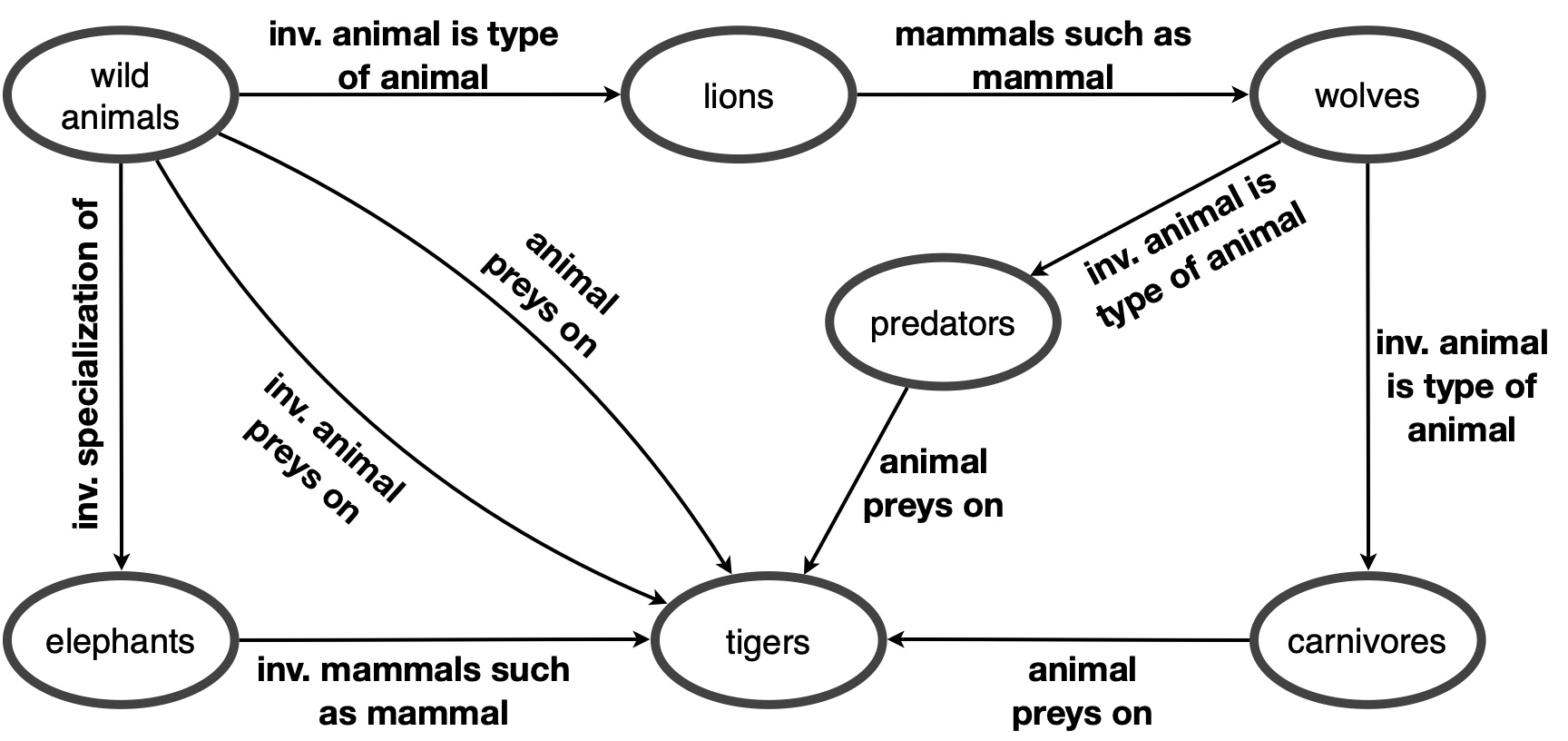
Figure 5. Example of a rule instantiation graph from NELL-995 v3, corresponding to the prediction of (wild animals, inv. animal is type of animal, tigers).

Example of a rule instantiation graph from NELL-995.

5.2. Analysis

Rare vs frequent relations

We found that the GNN-based aggregation methods can underperform when insufficient training data is available. A similar issue arises for relations that are too rare, even when the overall training graph is larger. To illustrate this, Figure 2 shows a break-down of the results (on the test set) for the 10% most frequent relations in the training graph (frequent) the next 40% most frequent relations (common) and the 50% least frequent relations (rare). We can see that the outperformance of CompGCN over AnyBURL is generally far more pronounced for frequent relations. This is as expected, since we need sufficient training data to learn the GNN models. However, for NELL-995 v2 and v3, we see the opposite behaviour, with CompGCN clearly underperforming AnyBURL for frequent relations. This discrepancy arises from the noisy nature of these datasets, which means that a high number of unreliable rules are being learned. A particularly clear-cut examples is provided in Figure 4, which shows a rule instantiation graph where the rules involved are essentially non-sensical. As another notable observation in Figure 2, we can see that the outperformance of CompGCN + NBFNet over CompGCN is most pronounced for rare relations (especially for the FB15k-237 and NELL-995 datasets). This is also as expected, since we have fewer rules for rare relations, making it more likely that the correct answer ends up in $\mathcal{B}_{q}$.

Rules offer weak evidence for WN18RR

For the WN18RR datasets, we found that the GNN-based rule aggregation strategies were able to outperform AnyBURL by a considerably margin. This reflects the fact that the available rules for these datasets offer relatively weak evidence. It therefore becomes more important to aggregate the evidence from multiple rule instantiations. The weak nature of the individual rules is illustrated in Figure 3, where we show a rule instantiation graph from WN18RR v1. Each of the rules individually only gives weak evidence, but the information encoded in the full rule instantiation graph nonetheless strongly suggests that there is a link between the two entities.

Rule aggregation is less successful for NELL-995

As we already mentioned, NELL-995 is much noisier than the other KGs, due to the fact that this dataset was extracted from text. Figure 5 illustrates this with an example from NELL-995 v3. In this case, most of the paths in the rule instantiation graph are not actually predictive (e.g. the fact that wild animals prey on tigers does not imply that tigers are a kind of wild animal). However, there are also rules which are somewhat more informative. For instance, the path in the bottom left corner expresses that tigers have something in common with elephants and that elephants are wild animals; this indeed provides us with some evidence for the inference that tigers could be wild animals. Due to the noisy nature of such rule instantiation graphs, focusing on the most reliable evidence (as done by AnyBURL) leads to better results than taking into account the entire rule instantiation graph.

6. Conclusions

We have analysed the performance gap between rule-based methods and GNNs for inductive KG completion. One important finding is that by reranking the entities which receive zero confidence by AnyBURL, we can significantly improve the performance of this rule-based method. We have also proposed to use a GNN to rerank the candidates predicted by AnyBURL. Rather than using the full knowledge graph, our GNN models only see the ground rules that predict each answer candidate. As such, their sole purpose is to aggregate the evidence provided by different AnyBURL rules. We found this strategy to be highly effective on several datasets. Together, these two modifications enable results which are close to those of NBFNet, while largely keeping the interpretability advantage of rule-based methods. We also analysed a variant in which NBFNet was used to rerank the candidated predicted by AnyBURL. This simple strategy allowed us to consistently outperform NBFNet. Finally, we have uncovered important methodological differences in how different inductive KG completion methods have been evaluated, meaning that published results are often incomparable.

References

- (1)
- Balazevic et al. (2019) Ivana Balazevic, Carl Allen, and Timothy M. Hospedales. 2019. TuckER: Tensor Factorization for Knowledge Graph Completion. In Proceedings of the 2019 Conference on Empirical Methods in Natural Language Processing and the 9th International Joint Conference on Natural Language Processing, EMNLP-IJCNLP 2019, Hong Kong, China, November 3-7, 2019, Kentaro Inui, Jing Jiang, Vincent Ng, and Xiaojun Wan (Eds.). Association for Computational Linguistics, 5184–5193. https://doi.org/10.18653/v1/D19-1522
- Betz et al. (2022) Patrick Betz, Christian Meilicke, and Heiner Stuckenschmidt. 2022. Supervised Knowledge Aggregation for Knowledge Graph Completion. In The Semantic Web - 19th International Conference, ESWC 2022, Hersonissos, Crete, Greece, May 29 - June 2, 2022, Proceedings (Lecture Notes in Computer Science, Vol. 13261), Paul Groth, Maria-Esther Vidal, Fabian M. Suchanek, Pedro A. Szekely, Pavan Kapanipathi, Catia Pesquita, Hala Skaf-Molli, and Minna Tamper (Eds.). Springer, 74–92. https://doi.org/10.1007/978-3-031-06981-9_5
- Bordes et al. (2013) Antoine Bordes, Nicolas Usunier, Alberto García-Durán, Jason Weston, and Oksana Yakhnenko. 2013. Translating Embeddings for Modeling Multi-relational Data. In Advances in Neural Information Processing Systems 26: 27th Annual Conference on Neural Information Processing Systems 2013. Proceedings of a meeting held December 5-8, 2013, Lake Tahoe, Nevada, United States, Christopher J. C. Burges, Léon Bottou, Zoubin Ghahramani, and Kilian Q. Weinberger (Eds.). 2787–2795. https://proceedings.neurips.cc/paper/2013/hash/1cecc7a77928ca8133fa24680a88d2f9-Abstract.html
- Chami et al. (2020) Ines Chami, Adva Wolf, Da-Cheng Juan, Frederic Sala, Sujith Ravi, and Christopher Ré. 2020. Low-Dimensional Hyperbolic Knowledge Graph Embeddings. In Proceedings of the 58th Annual Meeting of the Association for Computational Linguistics, ACL 2020, Online, July 5-10, 2020, Dan Jurafsky, Joyce Chai, Natalie Schluter, and Joel R. Tetreault (Eds.). Association for Computational Linguistics, 6901–6914. https://doi.org/10.18653/v1/2020.acl-main.617
- Chen et al. (2022) Yihong Chen, Pushkar Mishra, Luca Franceschi, Pasquale Minervini, Pontus Stenetorp, and Sebastian Riedel. 2022. ReFactor GNNs: Revisiting Factorisation-based Models from a Message-Passing Perspective. In NeurIPS. http://papers.nips.cc/paper_files/paper/2022/hash/66f7a3df255c47b2e72f30b310a7e44a-Abstract-Conference.html
- Das et al. (2018) Rajarshi Das, Shehzaad Dhuliawala, Manzil Zaheer, Luke Vilnis, Ishan Durugkar, Akshay Krishnamurthy, Alex Smola, and Andrew McCallum. 2018. Go for a Walk and Arrive at the Answer: Reasoning Over Paths in Knowledge Bases using Reinforcement Learning. In ICLR (Poster). OpenReview.net.
- Das et al. (2017) Rajarshi Das, Arvind Neelakantan, David Belanger, and Andrew McCallum. 2017. Chains of Reasoning over Entities, Relations, and Text using Recurrent Neural Networks. In EACL (1). Association for Computational Linguistics, 132–141.
- Galárraga et al. (2015) Luis Galárraga, Christina Teflioudi, Katja Hose, and Fabian M. Suchanek. 2015. Fast rule mining in ontological knowledge bases with AMIE+. VLDB J. 24, 6 (2015), 707–730.
- Galkin et al. (2022) Mikhail Galkin, Etienne G. Denis, Jiapeng Wu, and William L. Hamilton. 2022. NodePiece: Compositional and Parameter-Efficient Representations of Large Knowledge Graphs. In The Tenth International Conference on Learning Representations, ICLR 2022, Virtual Event, April 25-29, 2022. OpenReview.net. https://openreview.net/forum?id=xMJWUKJnFSw
- Hamilton (2020) William L. Hamilton. 2020. Graph Representation Learning. Morgan & Claypool Publishers.
- Lin et al. (2015) Yankai Lin, Zhiyuan Liu, Maosong Sun, Yang Liu, and Xuan Zhu. 2015. Learning Entity and Relation Embeddings for Knowledge Graph Completion. In Proceedings of the Twenty-Ninth AAAI Conference on Artificial Intelligence, January 25-30, 2015, Austin, Texas, USA, Blai Bonet and Sven Koenig (Eds.). AAAI Press, 2181–2187. http://www.aaai.org/ocs/index.php/AAAI/AAAI15/paper/view/9571
- Liu et al. (2021) Shuwen Liu, Bernardo Cuenca Grau, Ian Horrocks, and Egor V. Kostylev. 2021. INDIGO: GNN-Based Inductive Knowledge Graph Completion Using Pair-Wise Encoding. In NeurIPS. 2034–2045.
- Liu et al. (2022) Yang Liu, Zequn Sun, Guangyao Li, and Wei Hu. 2022. I Know What You Do Not Know: Knowledge Graph Embedding via Co-distillation Learning. In Proceedings of the 31st ACM International Conference on Information & Knowledge Management, Atlanta, GA, USA, October 17-21, 2022, Mohammad Al Hasan and Li Xiong (Eds.). ACM, 1329–1338. https://doi.org/10.1145/3511808.3557355
- Mai et al. (2021) Sijie Mai, Shuangjia Zheng, Yuedong Yang, and Haifeng Hu. 2021. Communicative Message Passing for Inductive Relation Reasoning. In AAAI. AAAI Press, 4294–4302.
- Markowitz et al. (2022) Elan Markowitz, Keshav Balasubramanian, Mehrnoosh Mirtaheri, Murali Annavaram, Aram Galstyan, and Greg Ver Steeg. 2022. StATIK: Structure and Text for Inductive Knowledge Graph Completion. In Findings of the Association for Computational Linguistics: NAACL 2022, Seattle, WA, United States, July 10-15, 2022, Marine Carpuat, Marie-Catherine de Marneffe, and Iván Vladimir Meza Ruíz (Eds.). Association for Computational Linguistics, 604–615. https://doi.org/10.18653/v1/2022.findings-naacl.46
- Meilicke et al. (2021) Christian Meilicke, Patrick Betz, and Heiner Stuckenschmidt. 2021. Why a Naive Way to Combine Symbolic and Latent Knowledge Base Completion Works Surprisingly Well. In AKBC.
- Meilicke et al. (2019) Christian Meilicke, Melisachew Wudage Chekol, Daniel Ruffinelli, and Heiner Stuckenschmidt. 2019. Anytime Bottom-Up Rule Learning for Knowledge Graph Completion. In Proceedings of the Twenty-Eighth International Joint Conference on Artificial Intelligence, IJCAI 2019, Macao, China, August 10-16, 2019, Sarit Kraus (Ed.). ijcai.org, 3137–3143. https://doi.org/10.24963/ijcai.2019/435
- Neelakantan et al. (2015) Arvind Neelakantan, Benjamin Roth, and Andrew McCallum. 2015. Compositional Vector Space Models for Knowledge Base Completion. In ACL (1). The Association for Computer Linguistics, 156–166.
- Omran et al. (2018) Pouya Ghiasnezhad Omran, Kewen Wang, and Zhe Wang. 2018. Scalable Rule Learning via Learning Representation. In IJCAI. ijcai.org, 2149–2155.
- Ott et al. (2021) Simon Ott, Christian Meilicke, and Matthias Samwald. 2021. SAFRAN: An interpretable, rule-based link prediction method outperforming embedding models. In 3rd Conference on Automated Knowledge Base Construction, AKBC 2021, Virtual, October 4-8, 2021, Danqi Chen, Jonathan Berant, Andrew McCallum, and Sameer Singh (Eds.). https://doi.org/10.24432/C5MK57
- Pirrò (2020) Giuseppe Pirrò. 2020. Relatedness and TBox-Driven Rule Learning in Large Knowledge Bases. In AAAI. AAAI Press, 2975–2982.
- Qu et al. (2021) Meng Qu, Junkun Chen, Louis-Pascal A. C. Xhonneux, Yoshua Bengio, and Jian Tang. 2021. RNNLogic: Learning Logic Rules for Reasoning on Knowledge Graphs. In 9th International Conference on Learning Representations, ICLR 2021, Virtual Event, Austria, May 3-7, 2021. OpenReview.net. https://openreview.net/forum?id=tGZu6DlbreV
- Sadeghian et al. (2019) Ali Sadeghian, Mohammadreza Armandpour, Patrick Ding, and Daisy Zhe Wang. 2019. DRUM: End-To-End Differentiable Rule Mining On Knowledge Graphs. In NeurIPS. 15321–15331.
- Schlichtkrull et al. (2018) Michael Sejr Schlichtkrull, Thomas N. Kipf, Peter Bloem, Rianne van den Berg, Ivan Titov, and Max Welling. 2018. Modeling Relational Data with Graph Convolutional Networks. In The Semantic Web - 15th International Conference, ESWC 2018, Heraklion, Crete, Greece, June 3-7, 2018, Proceedings (Lecture Notes in Computer Science, Vol. 10843), Aldo Gangemi, Roberto Navigli, Maria-Esther Vidal, Pascal Hitzler, Raphaël Troncy, Laura Hollink, Anna Tordai, and Mehwish Alam (Eds.). Springer, 593–607. https://doi.org/10.1007/978-3-319-93417-4_38
- Sun et al. (2019) Zhiqing Sun, Zhi-Hong Deng, Jian-Yun Nie, and Jian Tang. 2019. RotatE: Knowledge Graph Embedding by Relational Rotation in Complex Space. In 7th International Conference on Learning Representations, ICLR 2019, New Orleans, LA, USA, May 6-9, 2019. OpenReview.net. https://openreview.net/forum?id=HkgEQnRqYQ
- Teru et al. (2020) Komal K. Teru, Etienne G. Denis, and William L. Hamilton. 2020. Inductive Relation Prediction by Subgraph Reasoning. In Proceedings of the 37th International Conference on Machine Learning, ICML 2020, 13-18 July 2020, Virtual Event (Proceedings of Machine Learning Research, Vol. 119). PMLR, 9448–9457. http://proceedings.mlr.press/v119/teru20a.html
- Trouillon et al. (2016) Théo Trouillon, Johannes Welbl, Sebastian Riedel, Éric Gaussier, and Guillaume Bouchard. 2016. Complex Embeddings for Simple Link Prediction. In Proceedings of the 33nd International Conference on Machine Learning, ICML 2016, New York City, NY, USA, June 19-24, 2016 (JMLR Workshop and Conference Proceedings, Vol. 48), Maria-Florina Balcan and Kilian Q. Weinberger (Eds.). JMLR.org, 2071–2080. http://proceedings.mlr.press/v48/trouillon16.html
- Vashishth et al. (2020) Shikhar Vashishth, Soumya Sanyal, Vikram Nitin, and Partha P. Talukdar. 2020. Composition-based Multi-Relational Graph Convolutional Networks. In 8th International Conference on Learning Representations, ICLR 2020, Addis Ababa, Ethiopia, April 26-30, 2020. OpenReview.net. https://openreview.net/forum?id=BylA_C4tPr
- Wu et al. (2022) Hong Wu, Zhe Wang, Kewen Wang, and Yi-Dong Shen. 2022. Learning Typed Rules over Knowledge Graphs. In Proceedings of the 19th International Conference on Principles of Knowledge Representation and Reasoning, KR 2022, Haifa, Israel. July 31 - August 5, 2022, Gabriele Kern-Isberner, Gerhard Lakemeyer, and Thomas Meyer (Eds.). https://proceedings.kr.org/2022/51/
- Yan et al. (2022) Zuoyu Yan, Tengfei Ma, Liangcai Gao, Zhi Tang, and Chao Chen. 2022. Cycle Representation Learning for Inductive Relation Prediction. In ICML (Proceedings of Machine Learning Research, Vol. 162). PMLR, 24895–24910.
- Yang et al. (2015) Bishan Yang, Wen-tau Yih, Xiaodong He, Jianfeng Gao, and Li Deng. 2015. Embedding Entities and Relations for Learning and Inference in Knowledge Bases. In 3rd International Conference on Learning Representations, ICLR 2015, San Diego, CA, USA, May 7-9, 2015, Conference Track Proceedings, Yoshua Bengio and Yann LeCun (Eds.). http://arxiv.org/abs/1412.6575
- Yang et al. (2017) Fan Yang, Zhilin Yang, and William W. Cohen. 2017. Differentiable Learning of Logical Rules for Knowledge Base Reasoning. In NIPS. 2319–2328.
- Yao et al. (2019) Liang Yao, Chengsheng Mao, and Yuan Luo. 2019. KG-BERT: BERT for Knowledge Graph Completion. CoRR abs/1909.03193 (2019). arXiv:1909.03193 http://arxiv.org/abs/1909.03193
- Zhang et al. (2019) Shuai Zhang, Yi Tay, Lina Yao, and Qi Liu. 2019. Quaternion Knowledge Graph Embeddings. In Advances in Neural Information Processing Systems 32: Annual Conference on Neural Information Processing Systems 2019, NeurIPS 2019, December 8-14, 2019, Vancouver, BC, Canada, Hanna M. Wallach, Hugo Larochelle, Alina Beygelzimer, Florence d’Alché-Buc, Emily B. Fox, and Roman Garnett (Eds.). 2731–2741. https://proceedings.neurips.cc/paper/2019/hash/d961e9f236177d65d21100592edb0769-Abstract.html
- Zhang and Yao (2022) Yongqi Zhang and Quanming Yao. 2022. Knowledge Graph Reasoning with Relational Digraph. In WWW. ACM, 912–924.
- Zhang et al. (2022) Yongqi Zhang, Zhanke Zhou, Quanming Yao, Xiaowen Chu, and Bo Han. 2022. Learning Adaptive Propagation for Knowledge Graph Reasoning. CoRR abs/2205.15319 (2022).
- Zhang et al. (2020) Zhanqiu Zhang, Jianyu Cai, Yongdong Zhang, and Jie Wang. 2020. Learning Hierarchy-Aware Knowledge Graph Embeddings for Link Prediction. In The Thirty-Fourth AAAI Conference on Artificial Intelligence, AAAI 2020, The Thirty-Second Innovative Applications of Artificial Intelligence Conference, IAAI 2020, The Tenth AAAI Symposium on Educational Advances in Artificial Intelligence, EAAI 2020, New York, NY, USA, February 7-12, 2020. AAAI Press, 3065–3072. https://ojs.aaai.org/index.php/AAAI/article/view/5701
- Zhu et al. (2022) Zhaocheng Zhu, Xinyu Yuan, Louis-Pascal A. C. Xhonneux, Ming Zhang, Maxime Gazeau, and Jian Tang. 2022. Learning to Efficiently Propagate for Reasoning on Knowledge Graphs. CoRR abs/2206.04798 (2022).
- Zhu et al. (2021) Zhaocheng Zhu, Zuobai Zhang, Louis-Pascal A. C. Xhonneux, and Jian Tang. 2021. Neural Bellman-Ford Networks: A General Graph Neural Network Framework for Link Prediction. In Advances in Neural Information Processing Systems 34: Annual Conference on Neural Information Processing Systems 2021, NeurIPS 2021, December 6-14, 2021, virtual, Marc’Aurelio Ranzato, Alina Beygelzimer, Yann N. Dauphin, Percy Liang, and Jennifer Wortman Vaughan (Eds.). 29476–29490. https://proceedings.neurips.cc/paper/2021/hash/f6a673f09493afcd8b129a0bcf1cd5bc-Abstract.html