Understanding the Nature of the Optical Emission in Gamma-Ray Bursts: Analysis from TAROT, COATLI, and RATIR Observations

Abstract

We collected the optical light curve data of 227 gamma-ray bursts (GRBs) observed with the TAROT, COATLI, and RATIR telescopes. These consist of 133 detections and 94 upper limits. We constructed average light curves in the observer and rest frames in both X-rays (from Swift/XRT) and in the optical. Our analysis focused on investigating the observational and intrinsic properties of GRBs. Specifically, we examined observational properties, such as the optical brightness function of the GRBs at $T=1000$ seconds after the trigger, as well as the temporal slope of the afterglow. We also estimated the redshift distribution for the GRBs within our sample. Of the 227 GRBs analysed, we found that 116 had a measured redshift. Based on these data, we calculated a local rate of $\rho_{0}=0.2$ Gpc^-3 yr^-1 for these events with $z<1$. To explore the intrinsic properties of GRBs, we examined the average X-ray and optical light curves in the rest frame. We use the afterglowpy library to generate synthetic curves to constrain the parameters typical of the bright GRB jet, such as energy (${\langle}{E_{0}}{\rangle}\sim 10^{53.6}$ erg), opening angle (${\langle}\theta_{\mathrm{core}}{\rangle}\sim 0.2$ rad), and density (${\langle}n_{\mathrm{0}}{\rangle}\sim 10^{-2.1}$ cm^-3). Furthermore, we analyse microphysical parameters, including the fraction of thermal energy in accelerated electrons (${\langle}\epsilon_{e}{\rangle}\sim 10^{-1.37}$) and in the magnetic field (${\langle}\epsilon_{B}{\rangle}\sim 10^{-2.26}$), and the power-law index of the population of non-thermal electrons (${\langle}p{\rangle}\sim 2.2$).

1 Introduction

Gamma-ray bursts (GRBs) are the brightest electromagnetic events observed in the universe (O’Connor et al., 2023; Atteia et al., 2017). These bursts can be classified into two distinct populations: long GRBs (LGRBs) and short GRBs (SGRBs) (Kouveliotou et al., 1993). This classification is based primarily on the duration $T_{90}$, which represents the time interval that encompasses 90% of the total observed counts in gamma rays. LGRBs (with $T_{90}\gtrsim 2$ s) are associated with the collapse of massive stars (e.g., Woosley, 1993; MacFadyen & Woosley, 1999) whereas SGRBs (with $T_{90}\lesssim 2$ s) are believed to result from the coalescence of two compact objects (e.g., Paczynski, 1986, 1991; Lee & Ramirez-Ruiz, 2007; Abbott et al., 2017).

The fireball model (Sari et al., 1998) is the standard theory used to explain most of the features observed in the GRB light curves. This model describes both the prompt emission and the afterglow phase. During the prompt phase, the rapid variability is produced by internal shocks in the jet (Rees & Meszaros, 1994; Kobayashi et al., 1997), by photospheric emission (Thompson, 1994; Eichler & Levinson, 2000), or by magnetic reconnection (Zhang & Yan, 2011; Metzger et al., 2011). As the jet interacts with the circumburst medium, it decelerates, generating the afterglow phase. This phase is characterised by synchrotron emission, where relativistic electrons are continuously accelerated by an ongoing shock that interacts with the surrounding medium (Granot et al., 2002). This blast wave creates a forward shock that propagates through the surrounding medium and a reverse shock that propagates through the shell (Sari et al., 1998).

The emission of the afterglow can be described by power-law segments of the flux $F\propto t^{-\alpha}\nu^{-\beta}$, where $T$, $\nu$, $\alpha$, and $\beta$ represent time, frequency, temporal index, and spectral index (Granot et al., 2002; Sari et al., 1998).

With the launch of the Swift mission in 2004, our understanding of afterglows has greatly expanded (Gehrels et al., 2004). This is largely due to the monitoring provided by the X-Ray Telescope (XRT), which has provided an abundance of data from the very beginning of the afterglow. Unlike lower frequencies, the large amount of X-ray data has enabled both statistical studies and a in-depth investigations of the light curves of GRBs at these energies (Burrows et al., 2005).

The observational phases of X-ray afterglows can generally be identified as follows: a steep decay phase related to the end of the prompt emission phase; a shallow decay phase (or plateau) commonly interpreted as a signature of late-time energy injection; a normal decay phase; and a jet-break steepening given by a geometric effect related with the observer seeing the edge of the jet at late times. Additionally, flares are sometimes observed (see, e.g. Zhang et al., 2006; Nousek et al., 2006; Evans et al., 2009). These flares are believed to be produced by the central engine in a manner analogous to the prompt emission (Burrows et al., 2005).

However, observing the GRB early optical emission by ground telescopes is not an easy task. This is because gamma-ray bursts (in their prompt emission phase) are short-lived, lasting only a few seconds to a few minutes, and most ground-based telescopes simply cannot respond quickly enough to capture their first seconds. Moreover, the telemetry delays in receiving alerts from the General Coordinates Network/Transient Astronomy Network (GCN/TAN), result in the loss of early information from GRBs at these frequencies.

Therefore, the sample size of the early optical phases of the GRB remains considerably smaller compared to the later afterglows (see e.g. Wang et al., 2013; Li et al., 2012; Kann et al., 2010). Despite this limitation, these samples provide valuable insight into the diverse range of apparent brightness values observed during the early phases of GRBs. In some cases, extremely faint nearby GRBs have been observed (see e.g. Liang et al., 2007) while, in other cases, the observed brightness is much higher than expected (see e.g. Perley et al., 2014; O’Connor et al., 2023; Becerra et al., 2023), reaching apparent magnitudes of approximately $r=14$–16 (see e.g. Pereyra et al., 2022; Klotz et al., 2009). This suggests that the observed brightness is not solely dependent on the distance.

Moreover, not all GRBs have an optical counterpart, and the reason for this darkness has been widely discussed (see e.g. Greiner et al., 2011). Possible explanations have been proposed by Lang et al. (2010): i) the intrinsically low luminosity of the GRB; ii) the environment surrounding the GRB; and iii) the high absorption of intergalactic medium due to large distances ($z>6$).

Small aperture, fast slewing telescopes are usually used for observations of optical counterparts of GRBs (see e.g. Klotz et al., 2006; Becerra et al., 2019a), whereas larger aperture telescopes are necessary for detecting the afterglow when it has faded. In this paper, following this pattern, we use early optical data from the COATLI and TAROT telescopes and late data from RATIR (see, e.g. Becerra et al., 2019b). We aim to describe the observational properties of a sample of early optical afterglows followed by COATLI, TAROT, and RATIR. We describe each of them in § 2 and the complete sample in § 3. We present the phenomenological results in § 4: the brightness function at $T+1000$ s and the subsequent analysis at the early phases of the afterglow. In this section, we also compare the X-ray and optical flux to classify the events of our sample as dark or not. Additionally, we analyse the redshift distribution of our sample in § 5. Finally, we discuss and summarise our conclusions in § 6.

2 Telescopes

2.1 TAROT

The Télescopes à Action Rapide pour les Objets Transitoires (TAROT) are an automated telescope network located at different sites around the world with automated observations (without human interaction). TAROT was first designed as a robotic observatory in 1995. The Calern (TCA) observatory in France hosted the first TAROT, and its first light was in 1998. TAROT subsequently expanded to two other sites: La Silla, Chile (TCH) and La Reunión (TRE). TCA and TCH have a FoV 1.8$\times$ 1.8 square degrees, whereas the FoV of TRE is 4.2$\times$ 4.2 square degrees. TCA and TCH have a limiting $R$ magnitude of $R=18.2$ at 5$\sigma$ for unfiltered exposures of one minute, whereas the limiting magnitude of TRE is magnitudes of $R=17$. The goal of this consortium is the very early observations of GRB optical counterparts (Klotz et al., 2006). TAROT is connected to the GCN/TAN alert system and its first exposure is trailed with a duration of 60 seconds to allow continuous monitoring of the light curve. For these exposure, the tracking the hour-angle motor was adapted to give a drift of 0.30 pixels/s. As a consequence, stars trail with a length of about 18 pixels on the image and the flux is recorded continuously without dead time (Klotz et al., 2006). Subsequent exposures are typically conventional and do have a small amount of dead time.

2.2 COATLI

COATLI is an ASTELCO 50-cm Richey-Crétien telescope on a fast ASTELCO NTM-500 German equatorial mount at the Observatorio Astronómico Nacional on Sierra de San Pedro Mártir in Baja California, Mexico (Watson et al., 2016; Cuevas et al., 2016).

COATLI is connected to the GCN/TAN alert system and observes GRBs autonomously. The reduction pipeline (Becerra et al., 2019a) performs bias subtraction, dark subtraction, flat-field correction, and cosmic ray cleaning with the cosmicrays task in iraf (Tody, 1986). We perform astrometric calibration of our images using the astrometry.net software (Lang et al., 2010). We calibrate against USNO-B1 (Monet et al., 2003) and Pan-STARRS DR1 (Magnier et al., 2020).

The COATLI $w$ photometry is well described by $(w-r^{\prime})=0.353(g^{\prime}-r^{\prime})-0.243{(g^{\prime}-r^{\prime})}^{2}$ where the apostrophes in $g^{\prime}$ and $r^{\prime}$ refer to SDSS magnitudes (Becerra et al., 2019a).

2.3 RATIR

The Reonization and Transients Infrared/Optical Project (RATIR) was a four-channel simultaneous optical and near-infrared imager mounted on the 1.5 meters Harold L. Johnson Telescope at the Observatorio Astronómico Nacional in Sierra San Pedro Mártir in Baja California, Mexico. It was operated from 2012 April to 2022 June. RATIR responded autonomously to GRB triggers from the Swift/BAT instrument and obtained simultaneous photometry in $riZJ$ or $riYH$ (Butler et al., 2012; Watson et al., 2012; Littlejohns et al., 2015; Becerra et al., 2017).

The reduction pipeline (Littlejohns et al., 2015) performs bias subtraction and flat-field correction, followed by astrometric calibration using the astrometry.net software (Lang et al., 2010), iterative sky subtraction, co-addition using swarp (Bertin, 2010), and source detection using sextractor (Bertin & Arnouts, 1996). We calibrate against SDSS DR9 (Ahn et al., 2012) and 2MASS (Skrutskie et al., 2006).

3 Data sample

We used all available optical photometric data from TAROT, RATIR, and COATLI. TAROT and COATLI use clear filters, whereas the RATIR griZYJH photometry system. For typical GRBs, the AB magnitudes in the TAROT and COATLI clear filters ($w$-filters) are approximately the same as those in the RATIR $r$-filter (see e.g. Becerra et al., 2019b, c, 2021).

The complete information for each event is described in Table 3. The first column shows the name of the GRB, the second the Swift/BAT trigger, and the third, fourth, and fifth columns list the redshift z, the extinction value $E(B-V)$, and the duration $T_{90}$, respectively. The information on the redshift $z$, reddening $E(B-V)$, and duration $T_{90}$ was retrieved from the GCN/TAN circulars and the Swift/BAT repository. To calculate the extinction $A_{r}$, we use the relationship $A_{V}=3.1\times$$E(B-V)$ and (Schlegel et al., 1998) and $A_{r}/A_{V}\approx 0.9$ (Gordon et al., 2003). We illustrate the histograms of duration and redding in Figure 1. We include new COATLI photometry of GRB 180706A (see Table Understanding the Nature of the Optical Emission in Gamma-Ray Bursts: Analysis from TAROT, COATLI, and RATIR Observations) and GRB 180812A (see Table Understanding the Nature of the Optical Emission in Gamma-Ray Bursts: Analysis from TAROT, COATLI, and RATIR Observations).

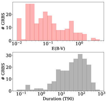
Figure 1: Histograms of reddening values $E(B-V)$ (top panel), and duration $T_{90}$ (bottom panel).

For the sample used in this study, we have 13 SGRBs and 205 LGRBs according to the parameter $T_{90}$. Furthermore, the Swift catalog gives redshifts for 116 out of 227 events, that is, 51% of the sample. To find out if this sample is representative of the total population of GRBs, we compared the cumulative distribution of the redshifts of GRBs detected in our sample (see Table 3) and the redshift values in the catalogue of all GRBs detected by the Swift/BAT instrument. We plot this comparison in Figure 2. The similarity between the two curves was quantified by a Kolmogorov-Smirnov test, which gavea p-value of 0.69. Therefore, we conclude that the two distributions are similar and that the results obtained in this work the population studied here is not biased in redshift with respect to the whole Swift sample. This distribution is analysed in detail in § 5.1.

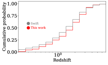
Figure 2: Comparison between the cumulative probability distribution of redshifts for the events in the sample used in this work and the redshifts of all GRBs in the Swift/BAT catalog.

4 Phenomenological Results

A total of 227 events were collected from the COATLI, RATIR and TAROT databases, of which 133 were detections, and the remaining 94 were only upper limits, all of which are shown in Figure 3. The first image was captured, on average, about 150 s after the trigger, with an initial AB magnitude of around $r=16.5$. In Figure 3, we also show the average optical light curve of prompt emission and early afterglow for GRBs (black line) with the corresponding $1\sigma$ deviation (grey regions).

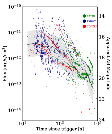
Figure 3: Optical detections and upper limits from TAROT (blue), RATIR (red) and COATLI (green) GRBs in the observed frame. Gray regions represent the 1$\sigma$ dispersion from the average curve (black line).

4.1 Brightness function

Akerlof & Swan (2007) and Klotz et al. (2009) investigated the brightness function of GRBs at $T=1000$ s. We adopt a similar approach here for the bright. We use only data between $T+500$ s and $T+2000$ s for interpolation (31 detections and 15 upper limits),compared to Akerlof & Swan (2007) who used the photometric information between $T+100$ s and $T+10000$ s, we refined our fit . For the cases where only a single data point (either detection or upper limit) was available, we estimate the magnitude at $T=1000$s using a power-law function $F\propto t^{-\alpha}$, with $\alpha=1$ (Gehrels et al., 2004). In the case where multiple upper limits were available for the same event, we use the deepest upper limit for the calculation.

Figure 4 presents the normalised cumulative probability histogram resulting from our analysis. We compare against a similar analysis performed with the data presented by Akerlof & Swan (2007) (see their Tables 1 and 2) . However, to account for the difference with the limiting magnitudes of the facilities involved in our and their analyses, we only consider their data when the detections or upper limits are brighter than $r=18.5$, which is the limiting magnitude of COATLI and TAROT with stacked images.

Following Klotz et al. (2009), we considered two scenarios for the upper limits: i) an optimistic scenario, in which we assume that the non-detections lie just below the observed limiting magnitude (continuous lines in Figure 4); ii) a pessimistic scenario, in which we assume that the non-detections are even fainter than the faintest detected afterglow (dashed lines in Figure 4). We also plot the average of these two scenarios (continuous thick lines in Figure 4).

Under these assumptions, by comparing our result with that obtained by Akerlof & Swan (2007) we see a striking similarity in the brightness distribution. We estimate that about 20% of the GRBs observed with telescopes such as COATLI or TAROT exhibit optical magnitude $r<$16 and 75% $r<$18.

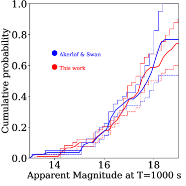
Figure 4: Cumulative optical brightness function obtained in this work at $T+1000$ seconds for the detections and upper limits. We used the same criteria for pessimistic (dashed lines) and optimistic (solid lines) scenarios described by Klotz et al. (2009) for this work Akerlof & Swan (2007) (blue). We also plot the mean distribution, for both samples in thicker solid lines.

4.2 Slope distribution

To gain further insight into the nature of the brightness function, we analyse the temporal index of the light curve determined for GRBs with more than one single point detected between $T+500$ s and $T+2000$ s. We fit a single power-law function to find the temporal index and the apparent magnitude at $T=1000$ s. We illustrate this in the left panel of Figure 5. We found that the average $\alpha$ for detections is $0.80\pm 0.61$ whereas the average apparent magnitude at 1000 s is $16.72\pm 1.36$. The uncertanities refer to the $1\sigma$ deviation from the average. The value of the temporal index is slightly larger than the one reported by Dainotti et al. (2022) and Srinivasaragavan et al. (2020) (at the end of the plateau phase). This is explained by the presence of flares, reverse shocks and optical rebrightenings that can be found at earlier times. Figure  5 shows no clear correlation, indicating that the afterglow decay rate is not a dominant parameter in the brightness of the early afterglow. We also determined in which phase of the light curve the GRBs are at time $T+1000$ s, in order to distinguish the origin of the brightness, i.e., if the emission is produced by the typical decay of an afterglow or instead is due to an additional component (reverse shock, late central activity, etc.). For subsequent analysis and discussion, we distinguish events with previously identified reverse shock (stars) or late central activity components (squares).The figure shows that there is no clear correlation between the phase of the light curve and and the observed magnitude.

The next step was to investigate the correlation between the apparent magnitude and the distance of the GRB. This is shown in the right panel of Figure 5. As might be expected, a slight trend is observed between the faintest and most distant GRBs. Nevertheless, the dispersion in the graph is too large to find a conclusive empirical relationship.

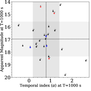
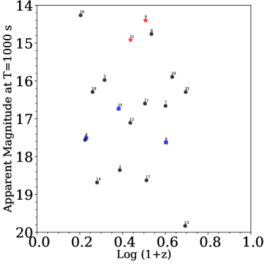
Figure 5: Left: Apparent optical magnitude vs temporal index $\alpha$ at $T+1000$ s. We plot the mean values for the apparent magnitude and the temporal index at that time (dashed black lines) and the $1\sigma$ dispersion (grey area). Right: Apparent optical magnitude at $T+1000$ s vs redshift. We distinguish the events with previously identified reverse shocks (red stars) or late central activity (blue squares). The numbers in the figure identify each GRB: 1. GRB 160127A, 2. GRB 180314A, 3. GRB 111209A, 4. GRB 060904B, 5. GRB 201021C, 6. GRB 070420, 7. GRB 141109A, 8. GRB 080413A, 9. GRB 110205A, 10. GRB 120913B, 11. GRB 210222B, 12. GRB 120119A, 13. GRB 120909A, 14. GRB 141225A, 15. GRB 130605A, 16. GRB 130215A, 17. GRB 180325A, 18. GRB 170519A, 19. GRB 180418A, 20. GRB 191016A, 21. GRB 210822A, 22. GRB 140419A, 23. GRB 150811A, 24. GRB 180812A, 25. GRB 180205A.

4.3 Dark GRBs

Since the first detections of the afterglows in the 1990s, it has been evident that X-rays and optical light curves do not follow a canonical pattern or exhibit a standard relationship. The GRBs which are bright in X-rays and subluminous in optical, or even completely lacking the optical counterpart are called dark GRBs. Fynbo et al. (2001); Lazzati et al. (2002) showed that a large fraction, about 60%-70%, of well-localised GRBs, has detections at optical wavelengths.

Lang et al. (2010) discussed three scenarios in which the optical emission is not present or is very weak compared to typical events: i) absorption by the host galaxy or the surrounding gas (e.g. see Djorgovski et al., 2001; Fynbo et al., 2001), ii) galactic absorption due to a high redshift, and iii) intrinsic faintness of some GRBs.

While instruments such as COATLI (and even more TAROT) do not have the sensitivity to detect dark GRBs, they can constrain the X-ray-to-optical flux ratio at early times. The comparison of this ratio with the bright-dark limit defined by Jakobsson et al. (2004) may indicate if early measurements with instruments like COALI or TAROT can quickly identify dark GRBs that require specific follow-up.

Jakobsson et al. (2004) proposed a definition of dark bursts based on the optical-to-X-ray spectral index $\beta_{\mathrm{ox}}<0.5$. This criterion has the advantage over others of leaving aside many of the factors, such as the collimation of the outflow and its density and depends on distance-independent properties of the burst rather than distance-dependent ones (see e.g. Djorgovski et al., 2001) and only considers how the optical counterpart is compared to the fireball model.

We used this criterion for our sample. Using the Swift/XRT light curve repository (Evans et al., 2007, 2009) hosted at the UK Swift Science Data Centre (UK SSDC), we selected only GRBs for which the X-ray data had a signal-to-noise ratio $S/N>3$ at $T=1000$ s. This cuts the sample from 227 to 34. For these, our optical photometry gives 21 detections and 13 upper limits at $T+1000$ s. These data are shown in Figure 6. We also identified the better constraint events (with an evident temporal evolution) with filled markers and suspicious ones with unfilled markers, whose behaviour in the interpolation is ambiguous because of the presence of a plateau, reverse shock, flare, etc. We also plot different dashed lines showing the corresponding spectral index between the optical and X-rays. The dark region, in which $\beta_{\mathrm{ox}}<0.5$, is shown in grey in the figure.

Figure 6 shows that all but one of the 34 GRBs lie above the bright-dark boundary, showing that the early identification of dark GRBs require instruments that are more sensitive than COATLI or TAROT. This will, however, become possible with COLIBRÍ, which reaches a limiting magnitude $R=22$ in 1000 s (Basa et al., 2022).

In our sample, the distance (and therefore the hydrogen absorption in the optical bands due to high redshifts) is not a problem. Likewise, only one of the GRBs in the sample (the ultra long GRB 111205A) is indisputably dark under this criterion (whereas the upper limits for GRB 141031A and GRB 070508 make them likely candidates). This GRB shows a very different duration and energy-fluence than any other observed (Gendre et al., 2013; Greiner et al., 2015). Therefore, it supports the idea that is had a different origin from the populations that produce the common long and short GRBs (Levan et al., 2014; Gendre et al., 2013; Greiner et al., 2015).

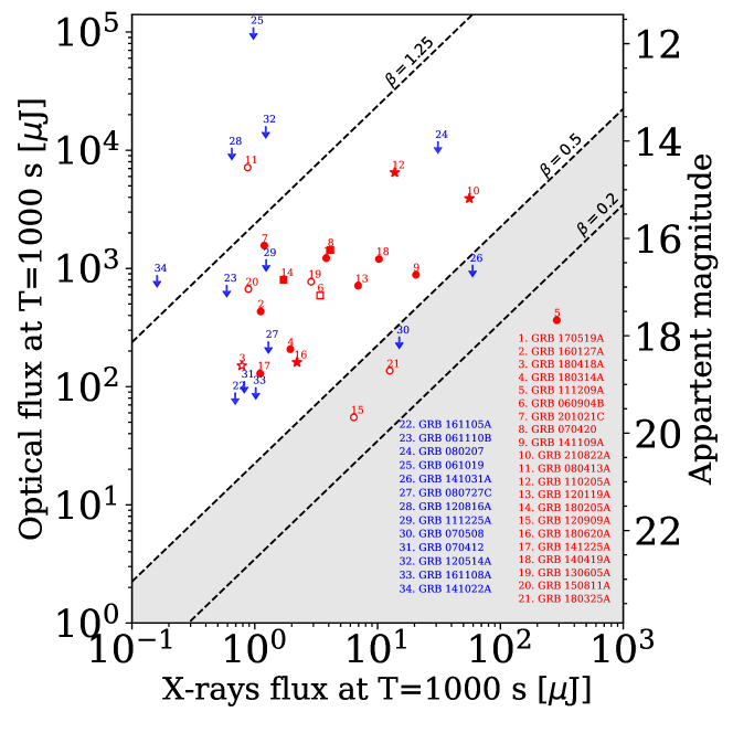
Figure 6: X-ray and optical fluxes at $T+1000$ s. We show detections (red) and the upper limits (blue). The empty markers refer to events whose interpolation in the X-ray time range is uncertain. We illustrate the criteria proposed by Jakobsson et al. (2004) to identify dark GRBs (dashed black lines) and the dark GRBs region (grey area). The dashed lines, in particular, correspond to different values of the optical-to-X-ray spectral index $\beta$.

5 Physical Results

5.1 Redshift distribution

We calculate the redshift distribution for those GRBS in our sample that have redshift determinations following Porciani & Madau (2001). The number density of GRBs at redshift z about z+dz is given by:

$$n(z)=\frac{dN}{dz}=\frac{R_{\mathrm{GRB}}(z)}{1+z}\frac{dV(z)}{dz}$$ (1)

where $R_{\mathrm{GRB}}(z)$ is the comoving GRB rate as a function of z, the factor $1/(1+z)$ accounts for the cosmological time dilation of the observed rate, and $\frac{dV(z)}{dz}$ is the comoving volume element. Assuming the star metallicity history from Kistler et al. (2008); Li (2008); Virgili et al. (2011),

$$R_{\mathrm{GRB}}(z)=\rho_{0}R_{\mathrm{SFR}}(z){(1+z)}^{\delta}\Theta(\epsilon,z)$$ (2)

where $\rho_{0}$ is the local GRB rate (in units of Gpc^-3yr^-1), $(1+z)^{\delta}$ accounts for the possible effect of evolution of the GRB rate exceeding the SFR rate, $\Theta(\epsilon,z)$ is the fractional mass density belonging to the metallicity below $\epsilon(Z_{\odot})$ at a given z and $(Z_{\odot})$ refers to the solar metal abundance). We use the star-forming rate $R_{\mathrm{SFR}}(z)$ reported by Porciani & Madau (2001) and Guetta & Piran (2007).

$${R_{\mathrm{SFR}}(z)=\rho_{0}\frac{23\exp{(3.4z)}}{\exp{(3.4z)}+22}}$$ (3)

$\Theta(\epsilon,z)$ is parameterized as Hopkins & Beacom (2006); Langer & Norman (2006)

$$\Theta(\epsilon,z)=\frac{\widehat{\Gamma}(\alpha+2,\epsilon^{\beta}10^{0.15\beta z})}{\Gamma(\alpha+2)}$$ (4)

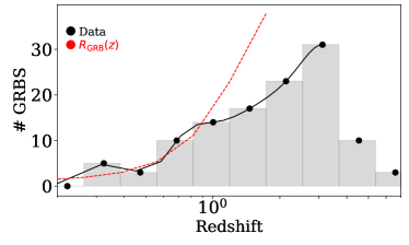
Figure 7: Histogram of the redshift distribution of our sample (gray bars) with the median data of each bin (black points) and a smoothing function for better visualization (black line). We fit a $R_{\mathrm{GRB}}(z)$ function (see in § 5.1) obtaining a $\rho_{0}=0.2$ Gpc^-3yr^-1 (dashed red line) with a $\chi^{2}=2.63$ for GRBs with redshift $z<1$. The information of redshifts was obtained from the Swift catalog.

where $\alpha=~{}-1.16$ is the power law index in the Schechter distribution function of galaxy stellar masses (Panter et al., 2004) and $\beta=~{}2$ is the slope in the linear bisector fit to the galaxy stellar mass-metallicity relation (Savaglio, 2006; Li, 2008), $\widehat{\Gamma}$ and $\Gamma$ the incomplete and complete gamma function, respectively, $\epsilon=0.4$, and $\delta=0.4$ (Li, 2008; Modjaz et al., 2008).

We fit equation 2 using TAROT, RATIR and COATLI data and the values/functions described previously. We estimate a GRB rate of $\rho_{0}=0.2$ Gpc^-3yr^-1 (dashed red line in Figure 7) with a $\chi^{2}=2.63$ for GRB with redshift $z<1$. This is only about 40% of the total number of GRBs expected to be detected per year $\rho_{0}=0.5-1.0$ (Zhang, 2018).

Previous studies have estimated the redshift-luminosity distribution of observed long Swift GRBs to obtain their rate and luminosity function. Wanderman & Piran (2010) described their sample with an increase for $0<z<3$ and a decrease for $z>3$. The same qualitative behaviour was obtained by Petrosian et al. (2015) using a non-parametric determination for 200 Swift long GRBs with known redshifts and by Yu et al. (2015) using Monte Carlo simulations.

Our results are consistent with the fact of COATLI and TAROT can only observe a fraction of GRBs because of factors such as weather, maintenance, and observatory closures. Furthermore, we sometimes do not observe GRBs that have previously reported magnitudes or upper limits that are below our sensitivity.

Our estimation illustrates the difficulties present in these predictions based on biased samples with uncertain selection effects, as has been discussed by Dainotti et al. (2021, 2015).

5.2 Canonical optical light curve

For each GRB in our sample with a redshift determination, we produced a rest-frame light curve, averaging the photometric information for each event over 20 equally spaced logarithmic intervals between the minimum and maximum values (see Figure 3). We corrected for Galactic extinction. To account for cosmological effects in our sample, we use the Cosmology calculator of Ned Wright (Wright, 2006). We assume a $\Lambda$CDM model with a $H_{0}=67.8$ $\mathrm{km\ s^{-1}\ Mpc^{-1}}$ (Planck Collaboration et al., 2014).

Figure 8 shows the rest-frame light curves. It also shows the average light curve as a solid line and the $1\sigma$ dispersion about this average. the $1\sigma$ error area in grey regions.

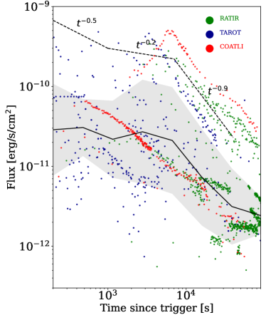
Figure 8: Optical detections from TAROT (blue), RATIR (green) and COATLI (red) GRBs in the rest frame and corrected for Galactic extinction. Gray regions represent the 1$\sigma$ dispersion about the average curve (black line). We also plot the canonical behaviour and the corresponding temporal indices (dashed line) estimated in this work.

Zhang et al. (2006) studies the X-ray light curves of GRBs and identified the different stages described in § 1. According to Zhang et al. (2006), the first part of the X-ray curve is likely related to tail emission of the prompt phase. After this initial decay, there is a plateau phase decay between $T=200$ s and $T=5000$ s. This segment suggests the presence of a continuing power source for the forward shock, which keeps being refreshed for some time. The most popular scenario is late central activity, that is, reactivation of the central engine. Nevertheless, it is not possible to reject other models such as a wide distribution of the shell Lorentz factors or the deceleration of a Poynting flux-dominated flow. That said, the presence of X-ray flares, around $T+1000$ s, suggests that the central engine is the source responsible for this continuing energy supply (Zhang et al., 2006). For $T>10000$, we observe the theoretically predicted normal decay.

Similarly, the optical light curve obtained in this study can be interpreted as follows:

• $T<1000$ seconds: Beginning of the optical emission. Compared with x-rays, the early times of the optical emission suggests a different origin for this phase and is therefore not linked to the end of the prompt phase or internal shocks. We observe the signature of a shallow decay with an average temporal index of $\alpha=-0.5$ for $T<1000$. This has been proposed to be the combination of reverse and forward shocks, such as in the cases of GRB 180418A (Becerra et al., 2019b), GRB 180620A (Becerra et al., 2019c) GRB 060904B, GRB 070420 (Klotz et al., 2008) GRB 110205 (Gendre et al., 2013; Steele et al., 2017).

• $1000<T<7000$ s: We find a shallow temporal decay with $\alpha=-0.2$ in this interval. Nevertheless, the large dispersion illustrates the variety of features present. This might have its origin in the energy released by late central engine activity that produces a plateau phase or an optical flare (see e.g. Kumar & Zhang, 2015; Zhang, 2018; Becerra et al., 2019a; Pereyra et al., 2022).

• $T>7000$ s: Optical counterpart of the normal decay observed in the X-ray canonical light curve, which is expected from the interaction between the head of the jet and the circumstellar medium. This has an average temporal index of $\alpha=-0.9$ (Kumar & Zhang, 2015; Zhang, 2018; Becerra et al., 2019c).

The phases identified here show the variety of processes and components that may be involved in early optical emission.

5.3 Parameters of the fireball model

The fireball model is typically used to describe the general behaviour of a GRB (Sari et al., 1998). This model relies on physical parameters of the jet such as energy $E_{0}$, angle of aperture $\theta_{\mathrm{core}}$, electron index $p$, and thermal energy fractions in electrons $\epsilon_{e}$ and in the magnetic field $\epsilon_{B}$ (Sari et al., 1998). Additionally, the density $n_{0}$ of the medium surrounding the progenitor must also be considered (Sari et al., 1998; Granot et al., 2002).

These variables are often degenerate and there are numerous combinations that could produce a given light curve. To constrain the physics of the jet, we used the library Afterglowpy (Ryan et al., 2020) to generate 100,000 different models with uniform random distributions of the parameters mentioned above. We assumed a structured jet for all the models (Urrutia et al., 2021; O’Connor et al., 2023) and compare with synthetic light curves that simultaneously deviated no more than $2\sigma$ from the average X-ray and optical light curves (see Figure 8) in the range between $T+200$ s and $T+50000$ s. The cumulative distribution functions of these constrained parameters are presented in Figure 9.

We determined the median values (corresponding to a cumulative probability of 0.5 in Figure 9) for these parameters as follows: the energy $E_{0}\approx 10^{53.6}$ erg, an opening angle $\theta_{\mathrm{core}}\sim 0.2$ rad, the density $n_{\mathrm{0}}\sim 10^{-2.1}$ cm^-3, $\epsilon_{e}\sim 10^{-1.37}$, magnetic field $\epsilon_{B}\sim 10^{-2.26}$, and the index of electrons $p\sim 2.2$, which are typical values for GRBs (see e.g. Fong et al., 2015; Santana et al., 2014; Berger, 2014; Levan et al., 2016) but the $\epsilon_{B}$ which is quite larger than previously measured (Santana et al., 2014).

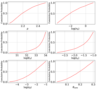
Figure 9: Cummultive distribution function (CDF) of the parameters obtained by simultaneously fitting the average X-ray and optical light curves (shown in Figure 8) using the AFTERGLOWPY (Ryan et al., 2020) library.

6 Discussion and summary

We presented optical photometry of the prompt emission and afterglow of GRBs that were observed by TAROT, COATLI, and RATIR up to 2022. We obtained an average light curve in both the observer frame and the rest frame. We divided the results into two main categories: phenomenological and physical.

For the first part, a brightness distribution of our sample is calculated and compared to the values reported by Akerlof & Swan (2007); Klotz et al. (2009) at $T+1000$ s. Nevertheless, the number of GRBs with reverse shock components or rebrightenings caused by late central activity makes it necessary to understand the behaviour of light curves beyond a simple decay. Therefore, we analyse the behaviour of the temporal indices for each GRB at this time. We observe a typical temporal index of $\alpha=0.80\pm 0.61$ for most of GRBs, but there are some cases where at that time a steeper decay (GRB 141225A) or a rapid rise (GRB 160127A and GRB 191016A) has been observed.

To investigate the nature of dark GRBs, we used the criterion proposed by Jakobsson et al. (2004), comparing the X-rays (from the Swift/XRT database) and optical fluxes at $T+1000$ s to evaluate how many of the optical fluxes correspond to those predicted under the fireball model.

Physically, using an analysis of the redshift distribution of our sample, we found a local GRB rate of $\rho_{0}=0.2$ Gpc^-3yr^-1 for GRBs with redshift $z<1$. Therefore, compared to the lowest theoretical predictions, these collaborations were only able to observe about 40% of the nearest GRBs.

Additionally, using the Afterglowpy library, we have determined a set of parameters (energy, opening angle, etc.) that deviate by a maximum of $2\sigma$ from the average canonical curve in X-rays and optical frequencies.

Although in this analysis we have worked with GRBs with cosmological and extinction corrections, this sample is limited by the instrumental characteristics of the instruments involved. For example, using photometry from other networks such as the Rapid Telescopes for Optical Response (RAPTOR) (Vestrand et al., 2002), the Mobile Astronomical System of TElescope Robots (MASTER) (Lipunov et al., 2010, 2022), the Katzman Automatic Imaging Telescope (KAIT) (Li et al., 2003) and the Burst Observer and Optical Transient Exploring System (BOOTES) (Castro-Tirado et al., 1999), we might have better coverage in terms of follow-up. Furthermore, given the sensitivities of each of these instruments, the databases could complement each other very well. In the future, we plan to expand this study using data available from these collaborations. Moreover, the community will also have the possibility to expand the understanding of earlier stages of GRBs with the arrival of the COLIBRÍ telescope (Fuentes-Fernández et al., 2020; Basa et al., 2022; Nouvel de la Flèche et al., 2022, 2023). This optical-infrared telescope will offer significantly improved sensitivity compared to COATLI or TAROT but a similarly fast response. This will enable the estimation of GRB’s redshift within minutes, making the upcoming years crucial for advancing our understanding of the GRB phenomenon.

Data availability

The data underlying this article will be shared on reasonable request to the corresponding author.

Table 1: COATLI Observations of GRB 180706A

$T$ ($s$)	Exposure ($s$)	$w$ (AB)
615	5	17.07$\pm$ 0.14
624	5	17.17$\pm$ 0.13
634	5	17.11$\pm$ 0.13

Table 2: COATLI Observations of GRB 180812A

References

- Abbott et al. (2017) Abbott B. P., et al., 2017, ApJ, 848, L13
- Ahn et al. (2012) Ahn C. P., et al., 2012, ApJS, 203, 21
- Akerlof & Swan (2007) Akerlof C. W., Swan H. F., 2007, ApJ, 671, 1868
- Anderson et al. (2018) Anderson M. M., et al., 2018, ApJ, 864, 22
- Atteia et al. (2017) Atteia J. L., et al., 2017, ApJ, 837, 119
- Basa et al. (2022) Basa S., et al., 2022, in Marshall H. K., Spyromilio J., Usuda T., eds, Society of Photo-Optical Instrumentation Engineers (SPIE) Conference Series Vol. 12182, Ground-based and Airborne Telescopes IX. p. 121821S, doi:10.1117/12.2627139
- Becerra et al. (2017) Becerra R. L., et al., 2017, ApJ, 837, 116
- Becerra et al. (2019a) Becerra R. L., et al., 2019a, ApJ, 872, 118
- Becerra et al. (2019b) Becerra R. L., et al., 2019b, ApJ, 881, 12
- Becerra et al. (2019c) Becerra R. L., et al., 2019c, ApJ, 887, 254
- Becerra et al. (2021) Becerra R. L., et al., 2021, ApJ, 908, 39
- Becerra et al. (2023) Becerra R. L., et al., 2023, MNRAS, 522, 5204
- Berger (2014) Berger E., 2014, ARA&A, 52, 43
- Bertin (2010) Bertin E., 2010, SWarp: Resampling and Co-adding FITS Images Together, Astrophysics Source Code Library, record ascl:1010.068 (ascl:1010.068)
- Bertin & Arnouts (1996) Bertin E., Arnouts S., 1996, A&AS, 117, 393
- Burrows et al. (2005) Burrows D. N., et al., 2005, Science, 309, 1833
- Butler et al. (2012) Butler N., et al., 2012, in McLean I. S., Ramsay S. K., Takami H., eds, Society of Photo-Optical Instrumentation Engineers (SPIE) Conference Series Vol. 8446, Ground-based and Airborne Instrumentation for Astronomy IV. p. 844610, doi:10.1117/12.926471
- Castro-Tirado et al. (1999) Castro-Tirado A. J., et al., 1999, A&AS, 138, 583
- Cuevas et al. (2016) Cuevas S., et al., 2016, in Evans C. J., Simard L., Takami H., eds, Society of Photo-Optical Instrumentation Engineers (SPIE) Conference Series Vol. 9908, Ground-based and Airborne Instrumentation for Astronomy VI. p. 99085Q, doi:10.1117/12.2234200
- Dainotti et al. (2015) Dainotti M. G., Del Vecchio R., Shigehiro N., Capozziello S., 2015, ApJ, 800, 31
- Dainotti et al. (2021) Dainotti M. G., Petrosian V., Bowden L., 2021, ApJ, 914, L40
- Dainotti et al. (2022) Dainotti M. G., Levine D., Fraija N., Warren D., Sourav S., 2022, ApJ, 940, 169
- Djorgovski et al. (2001) Djorgovski S. G., Frail D. A., Kulkarni S. R., Bloom J. S., Odewahn S. C., Diercks A., 2001, ApJ, 562, 654
- Eichler & Levinson (2000) Eichler D., Levinson A., 2000, ApJ, 529, 146
- Evans et al. (2007) Evans P. A., et al., 2007, A&A, 469, 379
- Evans et al. (2009) Evans P. A., et al., 2009, MNRAS, 397, 1177
- Fong et al. (2015) Fong W., Berger E., Margutti R., Zauderer B. A., 2015, ApJ, 815, 102
- Fuentes-Fernández et al. (2020) Fuentes-Fernández J., et al., 2020, Journal of Astronomical Instrumentation, 9, 2050001
- Fynbo et al. (2001) Fynbo J. U., et al., 2001, A&A, 369, 373
- Gehrels et al. (2004) Gehrels N., et al., 2004, ApJ, 611, 1005
- Gendre et al. (2013) Gendre B., et al., 2013, ApJ, 766, 30
- Gordon et al. (2003) Gordon K. D., Clayton G. C., Misselt K. A., Landolt A. U., Wolff M. J., 2003, ApJ, 594, 279
- Granot et al. (2002) Granot J., Panaitescu A., Kumar P., Woosley S. E., 2002, ApJ, 570, L61
- Greiner et al. (2011) Greiner J., et al., 2011, A&A, 526, A30
- Greiner et al. (2015) Greiner J., et al., 2015, Nature, 523, 189
- Guetta & Piran (2007) Guetta D., Piran T., 2007, J. Cosmology Astropart. Phys., 2007, 003
- Hopkins & Beacom (2006) Hopkins A. M., Beacom J. F., 2006, ApJ, 651, 142
- Jakobsson et al. (2004) Jakobsson P., Hjorth J., Fynbo J. P. U., Watson D., Pedersen K., Björnsson G., Gorosabel J., 2004, ApJ, 617, L21
- Kann et al. (2010) Kann D. A., et al., 2010, ApJ, 720, 1513
- Kistler et al. (2008) Kistler M. D., Yüksel H., Beacom J. F., Stanek K. Z., 2008, ApJ, 673, L119
- Klotz et al. (2006) Klotz A., Gendre B., Stratta G., Atteia J. L., Boër M., Malacrino F., Damerdji Y., Behrend R., 2006, A&A, 451, L39
- Klotz et al. (2008) Klotz A., Boër M., Eysseric J., Damerdji Y., Laas–Bourez M., Pollas C., Vachier F., 2008, PASP, 120, 1298
- Klotz et al. (2009) Klotz A., Boër M., Atteia J. L., Gendre B., 2009, AJ, 137, 4100
- Kobayashi et al. (1997) Kobayashi S., Piran T., Sari R., 1997, ApJ, 490, 92
- Kouveliotou et al. (1993) Kouveliotou C., Meegan C. A., Fishman G. J., Bhat N. P., Briggs M. S., Koshut T. M., Paciesas W. S., Pendleton G. N., 1993, ApJ, 413, L101
- Kumar & Zhang (2015) Kumar P., Zhang B., 2015, Phys. Rep., 561, 1
- Lang et al. (2010) Lang D., Hogg D. W., Mierle K., Blanton M., Roweis S., 2010, AJ, 139, 1782
- Langer & Norman (2006) Langer N., Norman C. A., 2006, ApJ, 638, L63
- Lazzati et al. (2002) Lazzati D., Covino S., Ghisellini G., 2002, MNRAS, 330, 583
- Lee & Ramirez-Ruiz (2007) Lee W. H., Ramirez-Ruiz E., 2007, New Journal of Physics, 9, 17
- Levan et al. (2014) Levan A. J., et al., 2014, ApJ, 781, 13
- Levan et al. (2016) Levan A., Crowther P., de Grijs R., Langer N., Xu D., Yoon S.-C., 2016, Space Sci. Rev., 202, 33
- Li (2008) Li L.-X., 2008, MNRAS, 388, 1487
- Li et al. (2003) Li W., Filippenko A. V., Chornock R., Jha S., 2003, PASP, 115, 844
- Li et al. (2012) Li L., et al., 2012, ApJ, 758, 27
- Liang et al. (2007) Liang E., Zhang B., Virgili F., Dai Z. G., 2007, ApJ, 662, 1111
- Lipunov et al. (2010) Lipunov V., et al., 2010, Advances in Astronomy, 2010, 349171
- Lipunov et al. (2022) Lipunov V. M., et al., 2022, Universe, 8, 271
- Littlejohns et al. (2015) Littlejohns O. M., et al., 2015, MNRAS, 449, 2919
- MacFadyen & Woosley (1999) MacFadyen A. I., Woosley S. E., 1999, ApJ, 524, 262
- Magnier et al. (2020) Magnier E. A., et al., 2020, ApJS, 251, 6
- Metzger et al. (2011) Metzger B. D., Giannios D., Thompson T. A., Bucciantini N., Quataert E., 2011, MNRAS, 413, 2031
- Modjaz et al. (2008) Modjaz M., et al., 2008, AJ, 135, 1136
- Monet et al. (2003) Monet D. G., et al., 2003, AJ, 125, 984
- Nousek et al. (2006) Nousek J. A., et al., 2006, ApJ, 642, 389
- Nouvel de la Flèche et al. (2022) Nouvel de la Flèche A., et al., 2022, in Holland A. D., Beletic J., eds, Society of Photo-Optical Instrumentation Engineers (SPIE) Conference Series Vol. 12191, X-Ray, Optical, and Infrared Detectors for Astronomy X. p. 121910Q (arXiv:2209.00386), doi:10.1117/12.2627826
- Nouvel de la Flèche et al. (2023) Nouvel de la Flèche A., et al., 2023, arXiv e-prints, p. arXiv:2306.03716
- O’Connor et al. (2023) O’Connor B., et al., 2023, arXiv e-prints, p. arXiv:2302.07906
- Paczynski (1986) Paczynski B., 1986, ApJ, 308, L43
- Paczynski (1991) Paczynski B., 1991, Acta Astron., 41, 257
- Panter et al. (2004) Panter B., Heavens A. F., Jimenez R., 2004, MNRAS, 355, 764
- Pereyra et al. (2022) Pereyra M., et al., 2022, MNRAS, 511, 6205
- Perley et al. (2014) Perley D. A., et al., 2014, ApJ, 781, 37
- Petrosian et al. (2015) Petrosian V., Kitanidis E., Kocevski D., 2015, ApJ, 806, 44
- Planck Collaboration et al. (2014) Planck Collaboration et al., 2014, A&A, 571, A1
- Porciani & Madau (2001) Porciani C., Madau P., 2001, ApJ, 548, 522
- Rees & Meszaros (1994) Rees M. J., Meszaros P., 1994, ApJ, 430, L93
- Ryan et al. (2020) Ryan G., van Eerten H., Piro L., Troja E., 2020, ApJ, 896, 166
- Santana et al. (2014) Santana R., Barniol Duran R., Kumar P., 2014, ApJ, 785, 29
- Sari et al. (1998) Sari R., Piran T., Narayan R., 1998, ApJ, 497, L17
- Savaglio (2006) Savaglio S., 2006, New Journal of Physics, 8, 195
- Schlegel et al. (1998) Schlegel D. J., Finkbeiner D. P., Davis M., 1998, ApJ, 500, 525
- Skrutskie et al. (2006) Skrutskie M. F., et al., 2006, AJ, 131, 1163
- Smith et al. (2021) Smith K. L., et al., 2021, ApJ, 911, 43
- Srinivasaragavan et al. (2020) Srinivasaragavan G. P., Dainotti M. G., Fraija N., Hernandez X., Nagataki S., Lenart A., Bowden L., Wagner R., 2020, ApJ, 903, 18
- Steele et al. (2017) Steele I. A., et al., 2017, ApJ, 843, 143
- Thompson (1994) Thompson C., 1994, MNRAS, 270, 480
- Tody (1986) Tody D., 1986, in Crawford D. L., ed., Society of Photo-Optical Instrumentation Engineers (SPIE) Conference Series Vol. 627, Instrumentation in astronomy VI. p. 733, doi:10.1117/12.968154
- Urrutia et al. (2021) Urrutia G., De Colle F., Murguia-Berthier A., Ramirez-Ruiz E., 2021, MNRAS, 503, 4363
- Vestrand et al. (2002) Vestrand W. T., et al., 2002, in Kibrick R. I., ed., Society of Photo-Optical Instrumentation Engineers (SPIE) Conference Series Vol. 4845, Advanced Global Communications Technologies for Astronomy II. pp 126–136 (arXiv:astro-ph/0209300), doi:10.1117/12.459515
- Virgili et al. (2011) Virgili F. J., Zhang B., Nagamine K., Choi J.-H., 2011, MNRAS, 417, 3025
- Wanderman & Piran (2010) Wanderman D., Piran T., 2010, MNRAS, 406, 1944
- Wang et al. (2013) Wang X.-G., Liang E.-W., Li L., Lu R.-J., Wei J.-Y., Zhang B., 2013, ApJ, 774, 132
- Watson et al. (2012) Watson A. M., et al., 2012, in Stepp L. M., Gilmozzi R., Hall H. J., eds, Society of Photo-Optical Instrumentation Engineers (SPIE) Conference Series Vol. 8444, Ground-based and Airborne Telescopes IV. p. 84445L, doi:10.1117/12.926927
- Watson et al. (2016) Watson A. M., et al., 2016, in Evans C. J., Simard L., Takami H., eds, Society of Photo-Optical Instrumentation Engineers (SPIE) Conference Series Vol. 9908, Ground-based and Airborne Instrumentation for Astronomy VI. p. 99085O (arXiv:1606.00690), doi:10.1117/12.2233000
- Woosley (1993) Woosley S. E., 1993, ApJ, 405, 273
- Wright (2006) Wright E. L., 2006, PASP, 118, 1711
- Yu et al. (2015) Yu H., Wang F. Y., Dai Z. G., Cheng K. S., 2015, ApJS, 218, 13
- Zhang (2018) Zhang B., 2018, The Physics of Gamma-Ray Bursts. Cambridge University Press, doi:10.1017/9781139226530
- Zhang & Yan (2011) Zhang B., Yan H., 2011, ApJ, 726, 90
- Zhang et al. (2006) Zhang B., Fan Y. Z., Dyks J., Kobayashi S., Mészáros P., Burrows D. N., Nousek J. A., Gehrels N., 2006, ApJ, 642, 354