Clusters in randomly-coloured spatial networks

Abstract

The behaviour and functioning of a variety of complex physical and biological systems depend on the spatial organisation of their constituent units, and on the presence and formation of clusters of functionally similar or related individuals. Here we study the properties of clusters in spatially-embedded networks where nodes are coloured according to a given colouring process. This characterisation will allow us to use spatial networks with uniformly-coloured nodes as a null-model against which the importance, relevance, and significance of clusters of related units in a given real-world system can be assessed. We show that even a uniform and uncorrelated random colouring process can generate coloured clusters of substantial size and interesting shapes, which can be distinguished by using some simple dynamical measures, like the average time needed for a random walk to escape from the cluster. We provide a mean-field approach to study the properties of those clusters in large two-dimensional lattices, and we show that the analytical treatment agrees very well with the numerical results.

I Introduction

The characterisation of spatial patterns, and the quantification of their significance, has pivotal importance in a variety of research and application fields, from urban studies to biology and ecology Papadimitriou2020 ; Barthelemy2022 . Indeed, the functioning of many physical and biological systems is intimately connected with their spatial organisation, and the emergence of certain characteristics and behaviours is almost inevitably underpinned or fostered by the presence (or development) of specific spatial patterns Traveset2012 ; Louf2014 ; Bassel2014 . One example is the emergence of social, economic, and ethnic segregation in urban areas Batty2005 ; Batty2013 ; Barthelemy2017 . The spatial arrangement of classes or categories throughout a city is normally far from uniform, and individuals belonging to the same social, economic, or ethnic group are very often found clustered in specific areas. As a result of these biases, modern cities normally look pretty fragmented or segregated at several meaningful scales, a condition that is often connected to social deprivation, uneven access to resources and services, and heterogeneous distribution of certain kinds of crimes  Bassolas2021 ; Bassolas2021bis . Another interesting example is the emergence of clusters in the development of mutants in biological systems, as in the case of cancerous masses, where the distribution, shape, and spatial organisation of those masses has been consistently associated with the aggressiveness of the tumour  Haughey2023 .

The presence of spatially-segregated clusters of units belonging to a certain class is normally seen as an interesting property of spatial complex systems per-se, under the assumption that a cluster is something that does not emerge naturally in a random, unorganised system. However, this hypothesis is seldom (if ever) tested against a suitable null-model, in order to associate a significance to the observed spatial fragmentation of a system under study. So we would generally accept that a city like London is segregated with respect to ethnicity, as we observe a quite uneven distribution of spatially-segregated ethnic groups across its metropolitan area, but there is no agreement about whether the situation in London is any better, or worse, or even comparable to the ethnic segregation observed, say, in Los Angeles or in San Francisco. This problem has been tackled in a series of recent works on the subject, which have striven to improve the objectivity of comparisons of structural indicators across different spatial systems Sousa2022 ; Bassolas2021 .

The aim of this paper is to characterise the shape, size, and geometric properties of the clusters of units emerging in spatial networks with coloured nodes. Because of their emergence from a similar random stochastic process, these clusters can be related to percolation clusters, and fall into a larger category of objects that are normally studied in different areas of mathematics and physics, such as polyominoes and lattice animals Golomb1994 ; Whittington1990 ; Xu2014 . The rationale behind our study is that the significance of an observed spatial pattern can only be assessed with respect to a sound null-model, and uniform random colourings provide a first-order null-model for that purpose. Our results show that relatively large connected clusters of nodes of a single colour are not at all that rare, even in the case of random uniform colouring processes. This means that the sheer size of a cluster might not be a good proxy for its significance, unless a proper comparison with a uniform random colouring process is carried out. We also show that the typical clusters emerging in random colourings are in general tree-like and very elongated, thus allowing us to employ the mean time needed for a random walk to exit a cluster as a proxy of its randomness. We also provide a mean-field theory that allows us to predict the expected size of clusters as the size of the underlying lattice increases.

II Clusters in coloured lattices

II.1 Notation

We call $\mathcal{G}$ a graph, or a network, defined as a pair ($\mathcal{N}$, $\mathcal{E}$) of the set of nodes $\mathcal{N}$ and the set $\mathcal{E}$ of pairs of nodes $(i,j)$, where each of these pairs represents an edge, i.e. a relationship, or a link, between the nodes $i$ and $j$ Latora2017 . For the purpose of this study, we only take into consideration spatial graphs Barthelemy2022 , whose nodes are associated with specific points in a given space and edges represent the connections or relationships among those locations, typically in terms of spatial proximity, adjacency, connectivity or transfer cost between the two corresponding points. We start by considering infinite two-dimensional square lattices, that are infinite graphs where each node $i$ is placed at one of the intersections $(x_{i},y_{i})$ of the grid of integer coordinates (i.e., $x_{i},y_{i}$ are integer numbers, for all values of $i$), and is connected to the four immediately adjacent nodes placed at a distance $1$ from it, i.e., the nodes at coordinates $(x_{i}-1,y_{i})$, $(x_{i}+1,y_{i})$, $(x_{i},y_{i}-1)$, and $(x_{i},y_{i}+1)$. Square lattices are widely used as a convenient model for studying spatial phenomena Kawano2019 ; Grujic2012 , and are largely studied also in the case of pattern analysis Meakin1986 ; Dill1995 . The main reason behind this choice is that, although they are a simple model of real-world spatial systems, square lattices are one of the most straightforward discretizations of the plane.

Since our main motivation is to provide a suitable and sound null-model for patterns observed in real-world spatial networks, we will consider in the following two concrete finite lattice geometries, namely grids and tori. A grid is a square lattice that has a finite size and a finite boundary. Nodes that are not in the boundary are connected to four neighbours, while nodes on the boundary will lack one or two neighbours (depending on whether they are placed on the side or on the corner of the lattice). As a result, not all nodes in a grid are structurally indistinguishable, and this fact has an impact on the estimation of the average properties of the system, especially when the size of the lattice is small. On the other hand, a torus is still a lattice with finite size, but it has periodic boundary conditions, effectively making all the nodes indistinguishable and eliminating heterogeneities due to boundary effects.

Each node $i$ of $\mathcal{G}$ is assigned a colour $c_{i}$, chosen from a set $C$ of available colours. In order to describe coloured patterns, we define a free cluster $\mathcal{C}$ as a maximal connected subgraph of $\mathcal{G}$ characterised by nodes of the same colour $c$. We call the size, or dimension, of a free cluster the number $N$ of nodes in $\mathcal{C}$. The shape of free clusters having the same size $N$ can vary considerably, depending on the relative position of the nodes belonging to it. We call cluster configuration, or simply cluster, a specific spatial arrangement of nodes of a free cluster at a given size $N$ (see Fig. 1(a)). In the case of lattices, we state that two clusters are distinct if their node positions cannot be obtained one from the other by translation, reflections, or rotation of node positions (or any combination of these spatial transformations). Notice that the number of different configurations of a free cluster with $N$ nodes is obviously finite, but still unknown in the case of clusters on square lattices for relatively small values of $N$ Silva2007 ; Shirakawa2012 ; Mason2023 .

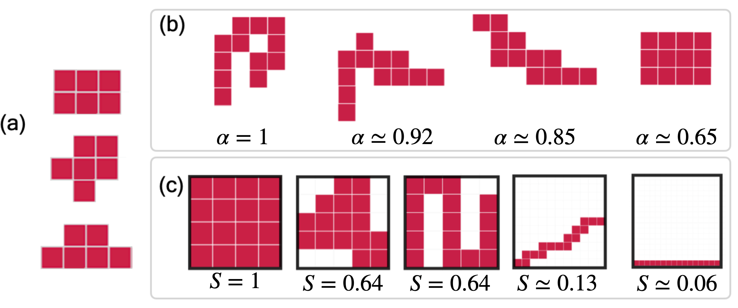
Figure 1: (a) Three distinct cluster configurations of the free cluster with $6$ nodes, where the edges of the cluster are represented by adjacency between nodes. (b) Four different cluster configurations of a free cluster with size $N=12$. The corresponding value of tree-likeness $\alpha$ is shown right beneath each configuration, and the configurations are ordered accordingly to their $\alpha$: the leftmost configuration is the one with the highest value of tree-likeness in the set. (c) Five different cluster configurations for the same free cluster with dimension $N=16$, along with their shape factor $S$. The configuration with the largest value of $S$ in the set is the leftmost one.

The different cluster configurations associated with a free cluster of size $N$ can be distinguished by a variety of structural properties. The most basic one is the number $e$ of edges connecting all the nodes of a cluster configuration, which obviously depends on the relative positions of the nodes belonging to the cluster. We define the surface $\sigma$ of a cluster the number of edges between the nodes in the cluster and the rest of the graph, i.e., all the nodes adjacent to nodes of the cluster that are of a different colour from that of the cluster. Among all the possible cluster configurations with a given size $N$, clusters with a small surface are indeed the more compact ones, i.e., whose nodes are more frequently connected to nodes in the cluster, rather than outside of the cluster. This preference has an obvious impact on the shape of a cluster configuration.

Another property of a cluster configuration that is connected to its structure and geometry is the so-called tree-likeness Cook1970 ; Potebnia2018 . For the purpose of this work, we define the tree-likeness $\alpha$ of a cluster configuration as the ratio between $N-1$ and the number $e$ of its edges. Indeed, the maximum value of $\alpha$ is $1$, as the cluster is by definition connected, and the minimum number of edges in a connected graph of $N$ nodes is $N-1$.

It is easy to show that $\alpha>0.5$ in the case of square lattice grids and tori. Since we are in a 2D lattice, which is obviously a planar graph Trudeau1993 ; Barthelemy2017b , there is exactly one edge between any pair of nodes that are adjacent on the lattice (and only among those nodes that are adjacent in the lattice). The consideration of finite lattices implies a finite number of edges, bounded by a value dependent on the lattice’s size, and it is related to the number of edges in the largest possible cluster within that lattice. For a torus with size $N$, the largest cluster that we can imagine has a size equal to that of the entire torus, and the number of edges in this cluster is precisely $2N$. For a grid with the same size, the largest possible cluster also covers the entire lattice. However, at difference with the torus, we need to consider the edges that were excluded from the count due to the torus boundary conditions. So in the end, for the largest cluster in the grid we have $2N-2\sqrt{N}$ edges. Since $2N-2\sqrt{N}<2N$, we have that the tree-likeness of a generic cluster with size smaller or equal to $N$ is bounded from below as follows:

$$\alpha\geq\frac{N-1}{2N}$$ (1)

and for $N\to\infty$ this lower bounds tends to $0.5$. So, in the case of finite square lattice grids and tori, for a cluster with size $N$, $\alpha$ takes values in the range $[\frac{1}{2}-\frac{1}{2N},1]$. In Fig. 1(b) we show some cluster configurations and the associated values of $\alpha$ for $N=12$. Note that values of tree-likeness close to $1$ indicate stripy or pitted clusters, while more compact configurations have a value of $\alpha$ close to $0.5$.

Finally, we define the shape factor $S$ of a cluster configuration as the ratio between the number of nodes in the cluster and the number of nodes in a pre-defined convex bounding box that contains the cluster completely Harris1964 ; Polsby1991 ; Wenwen2022 ; Montero2020 ; Wirth2020 . In this study, we consider as a bounding box the square with side equal to $D_{S}=1+\max\left\{\max_{i,j}\left\{|x_{i}-x_{j}|\right\},\max_{i,j}\left\{|y_{i}-y_{j}|\right\}\right\}$, where $(x_{i},y_{i})$ are the lattice coordinates of all the nodes $i$ belonging to the cluster. In Fig. 1(c) we show different cluster configurations for $N=16$ with their bounding box and shape factor. At fixed $N$, the more elongated the cluster, the larger its bounding box and the smaller the shape factor. For our definition of shape factor, the configuration with the highest $S$ is indeed the one corresponding to a square with side $\sqrt{N}$. We loosely call dense a cluster with a shape factor close to $1$, while clusters with a shape factor close to zero are called elongated, for obvious reasons. Similarly, for a fixed value of $N$, the cluster with the smallest possible shape factor in a square lattice (i.e., the most elongated one), is a line of nodes all having the same $x$ or $y$ coordinates, which yields $S=1/N$ (see the rightmost sub-plot of Fig. 1(c). This means that the shape factor of such lines effectively tends to $0$ as $N$ grows.

III Colouring processes

Graph colouring is a topic that affects many different scientific areas, including computer science, operations research, scheduling, and biology Kubale2004 ; Behnamian2016 ; Sudev2020 . Indeed, it is only by colouring or labelling nodes according to their function that we can often recognise the emergence of interesting patterns in a complex system, where interesting is any structure that hints to the emergence of a spontaneous or orchestrated organisation Papadimitriou2020 . A colouring over the set of nodes of a graph $\mathcal{G}$ is a function that assigns to each node one of the available colours or labels in a set $C$ of discrete elements, with size $|C|$. The assignment can be performed in many different (and arbitrary) ways and is often a random process associated with an underlying colour distribution IP .

III.1 The Uniform Random Colouring Process and the Random Growth Model.

We consider here the Uniform Random Colouring (URC ) process, as a specific colouring process that assigns to each node of the network $\mathcal{G}$ one of the available colours by randomly sampling it from a pre-determined colour distribution IP . In the URC process, the colour assigned to each node is independent from the colour of any other node of the graph: given a set $C$ of available colours, the distribution IP defines the probability for a node in the network to be coloured with the colour $c\in C$. The URC process is indeed the simplest stochastic process that preserves a given distribution of colours, without introducing correlations among colours. Since we are interested in assessing the significance of coloured clusters in a spatial network, and how the formation of spatial clusters entails the creation of some degree of correlation in the colours of adjacent nodes, we propose to use the URC process as a minimalist null-model against which the importance of correlations and heterogeneity in a spatial network with coloured nodes can be quantified.

In the following, we study how the structural properties of an URC cluster, including its size, shape, and compactness, depend on the size of the underlying graph $\mathcal{G}$ and on the number of available colours. To this aim, it is convenient to consider an analogous of the URC model as a growth process that obtains coloured clusters one by one, starting from an initial seed. In this way, we can obtain many clusters of prescribed size at the same time. We call this growing process the Random Growth Model (RGM ). Growth models are commonly used in many areas of applied mathematics and physics Eden1998 ; Turner2019 ; Candia2001 ; Jiang1989 ; Damron2018 , and can provide a framework for understanding how complex systems evolve and change over time, e.g., in response to external changes or stimuli. We call a cluster growth process a specific colouring over $\mathcal{G}$, where the assignment of colours over the nodes follows a specific colouring function, i.e. a growth rule, and the growth starts from a single node, or seed, assigned with a specific colour $c$, where we mark the seed with the label "$\times$", and all the other nodes are $blank$, i.e. nodes that have not yet been coloured. A cluster growth process starts from the first growth step, i.e. $t=0$, ad it proceeds by applying the growth rules for $t>0$ until the process stops. Usually, the rule specifies which adjacent blank nodes are eligible to be coloured at the next step $t$ by the colouring function, and we call random growth models such growth processes that assign colours to nodes in $\mathcal{G}$ following a stochastic colouring function.

In RGM the growth starts from a graph $\mathcal{G}$ where only one node is assigned with colour $c\in C$, as shown in Fig. 2(a) in the case where the graph $\mathcal{G}$ is a squared lattice. This single first node is the seed of our growing cluster. At each subsequent step $t$, we sample a colour from $C$ for each of the nodes adjacent to nodes in the cluster, according to the pre-determined colour distribution IP . If at least one of the adjacent nodes of the current cluster is assigned colour $c$, then the cluster has grown (since it has acquired at least one node), and the process can continue. Otherwise, there is no possibility for the cluster to grow further, as all the neighbours of the seed are assigned a colour different from $c$, and the process terminates. Notice that, since the assignment of colours to nodes is performed in a random and independent way, still according to the underlying colour distribution IP , the ensemble of clusters generated by RGM is equivalent to the ensemble of clusters generated by the URC process in a lattice whose size $N$ goes to infinity. As we will see in the following, RGM is a computationally more convenient way to study the behaviour of uniform random colouring as their sizes increases, so we will refer to URC and RGM interchangeably, as the only difference between the two models is the actual algorithm used to generate clusters with them.

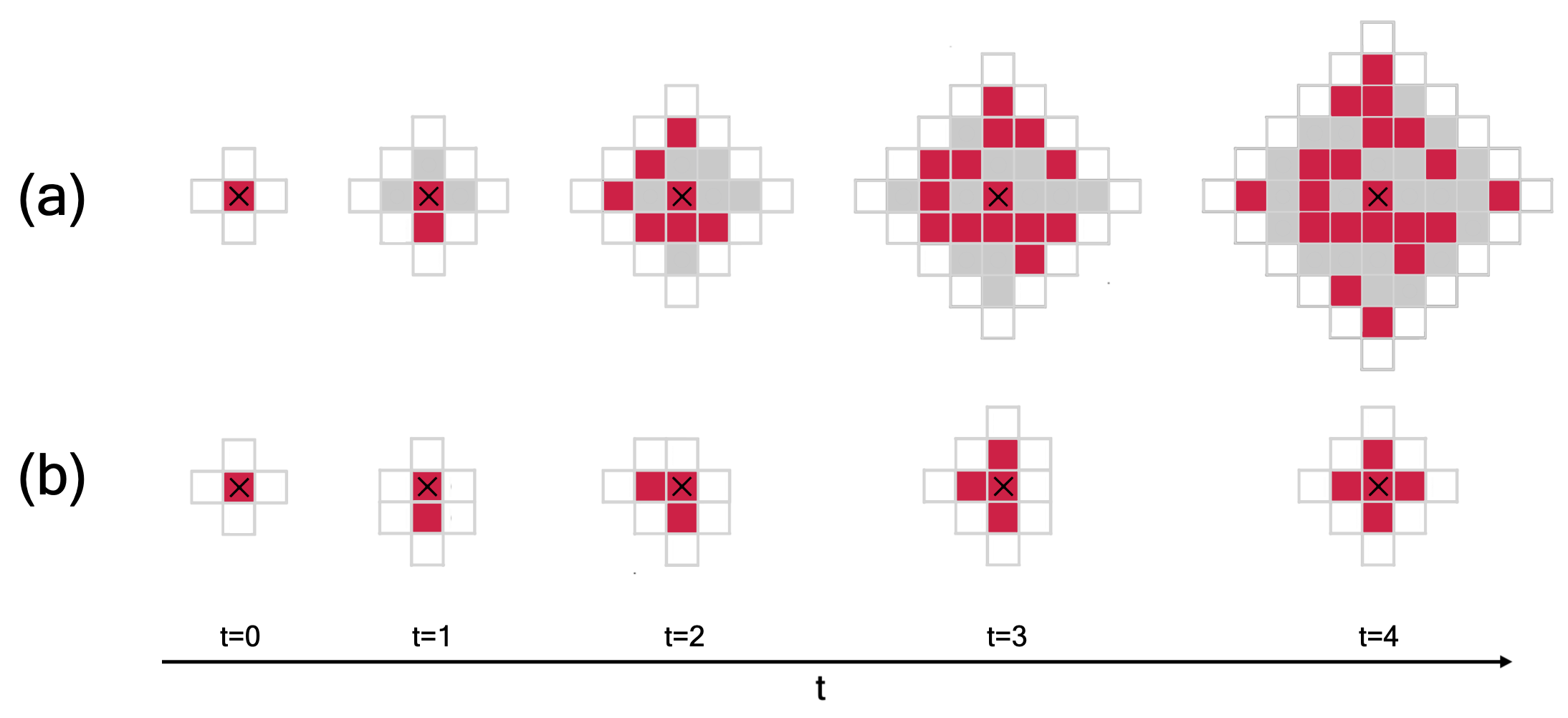
Figure 2: (a) One instance of RGM for five growth steps. At $t=0$, the seed cluster (labelled as "$\times$"), has only one node and is surrounded by blank nodes. Here we only show the blank nodes that are one step away from the coloured cluster. At $t=3$, the seed cluster grows considerably by acquiring several new nodes. When all the blank sites adjacent to the cluster are assigned with a colour different from the one of the cluster, the cluster can not grow anymore, as it happens in this case for $t=4$. (b) One instance of EGM is shown for five growth steps. The seed cluster is labelled as "$\times$", while only blank nodes that are one step away from the coloured subgraph are shown for each growth step. Note that an EGM cluster grows by one node at each step, with probability 1.

III.2 Correlated clusters and the Eden Growth Model.

As we aim to characterise coloured patterns, we choose to compare the RGM clusters with the ones produced by a growth model which is very well known in the literature, as it is largely used to study plant formation and bacterial growth, and to model a variety of biological systems: the Eden Growth Model (EGM ). Many variations of this growth process have been studied for shaping and modelling the natural realms in many different fields of study James2004 ; Frey2020 ; Ivanenko1999 ; Agyingi2018 . Here, we consider the first and most basic formulation of EGM , which produces an ensemble of motifs with a limiting shape tending to a circle when the size $N$ grows to infinity Manin2023 . In EGM , the growth starts from a blank graph with a coloured seed cluster of one node labelled with colour $c$, as in the case of RGM (Fig. 2(b)). At each time step $t$, one of the edges between the seed and the blank nodes is chosen uniformly at random, and the blank node connected with that chosen edge is assigned with colour $c$ with probability $p=1$. Notice that this rule forces a cluster to continue growing indefinitely, as each step of the model adds a new node to the existing cluster. This is fundamentally different from the case of RGM , as in that case the growth might die at any step.

Despite its elegant simplicity, the first formulation of the Eden Growth Model is still extensively used in many scientific fields, including urban growth and biology, to model the emergence of circle-like spatial arrangements Teknomo2005 ; Waclaw2015 ; Santalla2018 . In this model, the probability for a node to acquire a given colour does depend on the colour of its neighbours, and on the diffusion rule. Hence, the clusters generated by EGM exhibit quite strong spatial correlations. We will mainly use the EGM process to test the robustness and descriptiveness of our measures and also to make comparisons with the clusters obtained with the RGM growth, which instead are, by definition, uncorrelated.

IV Results

IV.1 Cluster size on grid and torus.

Here we show the properties of coloured clusters obtained by the URC model on finite grids and tori. We start from a uniform distribution of colours, meaning that the probability of assigning colour $c$ to each node is equal to $p=1/|C|$. We ran a large number ($5\times 10^{4}$) of simulations of the URC process on each type of graph, collecting the size of all the clusters across all the realisations. For our study, we choose graphs with size $4\times 10^{6}$. As we can see from Fig. 3(a), for $|C|=2$ we have a higher chance of observing clusters with a larger size than in the case of a different number of available colours. For $|C|=3$, the largest size observable is around $10^{2}$, and for $|C|=4$ and $|C|=5$ the largest size decreases even more. These results are in agreement with percolation theory on square lattices Newman2000 ; Mertens2022 . So, except for the singular case of $|C|=2$, we can conclude that the probability of observing extensive clusters on a grid or a torus is indeed an exponentially decreasing function of the cluster size $N$.

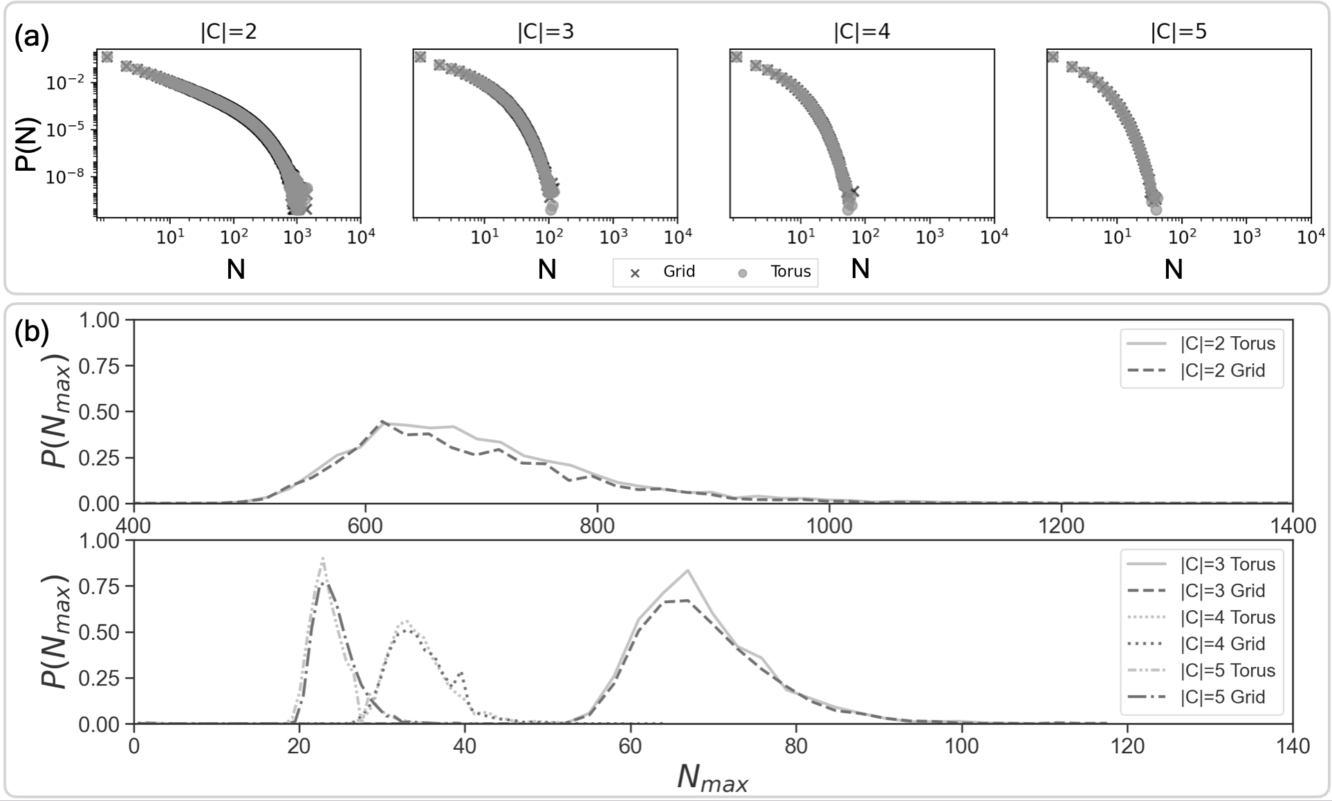
Figure 3: (a) Probability distribution $P(N)$ of the cluster size $N$ for a URC process run over a grid (dark grey) and a torus (light grey), for different values of $|C|$. (b) Probability distribution $P(N_{max})$ of the size $N_{max}$ of the largest cluster in the URC ensemble on a grid (dark grey) and a torus (light grey) with the same dimension. The case $|C|=2$ is shown in the top panel, while in the panel below the cases $|C|=3$, $|C|=4$, and $|C|=5$ are depicted. Notice that the number of colours has an impact on both the distribution of sizes and, more importantly, on the size of the largest cluster. All the distributions are computed over $5\times 10^{4}$ realisation of he corresponding model over tori or grids with $4\times 10^{6}$ nodes.

IV.2 The largest cluster in the URC process.

The size of the largest cluster obtainable on a lattice of a given size remains a subject of limited knowledge. Indeed, the size of a maximal cluster depends on a multitude of factors that have yet to be fully comprehended Zierenberg2017 . We now discuss the results of $5\times 10^{4}$ numerical simulations to obtain the distribution of the size of the largest URC cluster on a lattice. We obtained the largest cluster size $N_{max}$ for clusters on both grid and torus with side $D=2000$ (i.e., with $4\times 10^{6}$ nodes), and we look at the distribution of $N_{max}$ for different values of $|C|$. The position and the value of the peak of the distributions strictly depend on $|C|$ (Fig. 3(b)). The higher the value of $|C|$, the more the peak appears to shift to the left, meaning that the probability of obtaining large clusters in a URC with a large number of colours is smaller. The size of these clusters depends on the number of colours available, and it becomes quite irrelevant when compared to the overall size of the torus when $|C|$ increases. Despite the largest URC cluster being normally smaller than the overall graph, there remains a substantial probability of encountering clusters with relatively significant size, especially for $|C|=2$ (see Fig. 3(b)). This is indeed the most interesting scenario in the case of a URC process, as collecting large clusters in this case is somehow easier. Therefore, in the following we will only focus on clusters generated with a URC colouring in which $|C|=2$ and the probability of assigning one of the two available colours (namely $c$ and $c*$) is the same and equal to $p=\frac{1}{2}$.

IV.3 Tree-likeness and Shapefactor

In Fig. 4(a), we show the tree-likeness $\alpha$ for RGM and EGM clusters in the size range $N=[100,700]$ (top) and for the EGM clusters (bottom) with $N$ up to $10^{5}$. As shown in the top panel of Fig. 4(a), RGM clusters present a tree-likeness close to $0.8$, which is indicative of an essentially stripy shape. On the other hand, the EGM clusters exhibit smaller values of $\alpha$, reaching the limit value of $\alpha=0.5$ for large $N$ (see Fig. 4(a), bottom) as expected for the compact, filled, circle-shaped structures generated by the Eden Growth model.

In Fig. 4(b), we report the distribution of cluster shape factor over $10^{5}$ realisations of RGM and EGM clusters for different values of $N$. The peak of the distribution shifts to the left for the RGM clusters when $N$ increases. This means that RGM generates elongated clusters rather than dense ones as their size grows. On the contrary, in the case of EGM , the peak shifts in the opposite direction, meaning that the shape factor is increasing with size, and reaching the value of shape factor for the limiting shape of EGM clusters, which is the one of a circle. In fact, for a circle-like shape in a bounding box with side $2R$, we have that the shape factor is equal to:

$$S=\frac{\pi R^{2}}{(2R)^{2}}=\frac{\pi}{4}\simeq 0.78$$

which is around the value of the shape factor we measured for the peak of the EGM clusters at $N=10^{5}$. So, the shape factor is correctly telling us that EGM clusters shape is tending to the one of a circle when $N$ increases.

The difference in the range of cluster sizes between the two models, as made evident in Fig. 4(b), is due to the different rates at which clusters with a fixed dimension $N$ are generated: in the case of RGM clusters, because of the lower probability in observing large clusters, generating a statistically significant number of clusters in the dimension range $N=[10^{3},10^{5}]$ is comparatively harder - so the need to find another approach for describing the limiting shape of these objects.

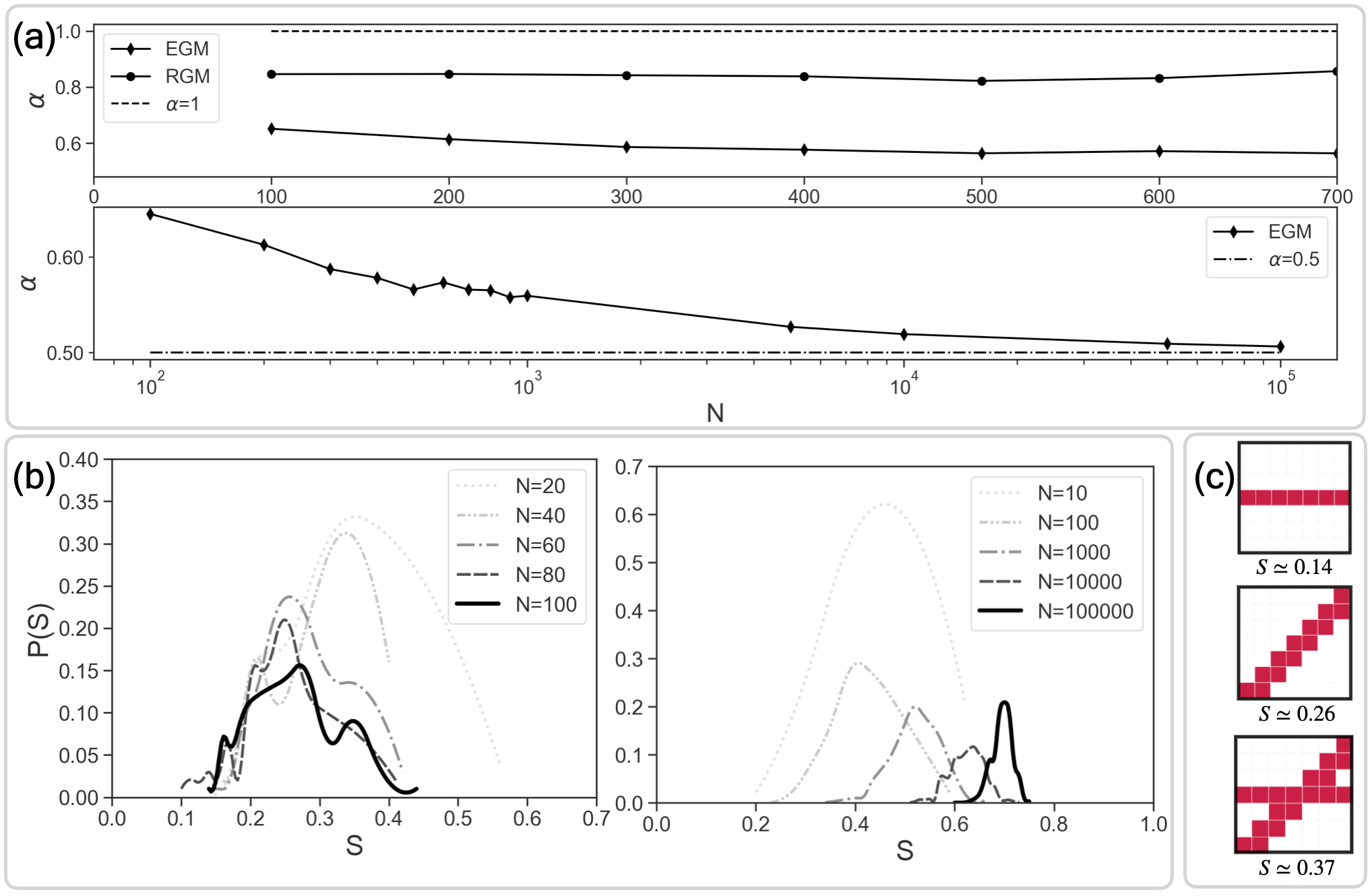
Figure 4: (a) Values of tree-likeness $\alpha$ for RGM and EGM clusters for $N$ in the range $N=[100,700]$ (top) and for EGM clusters (bottom) for $N\in[10^{2},10^{5}]$. The two panels also show the reference values $\alpha=1$ and $\alpha=0.5$. (b) Shape factor distribution $P(S)$ for RGM (left) and EGM (right) clusters. (c) The three typical and more probable local arrangements of RGM clusters, where the side of the domains in this case is $L=7$. The upper and the central domains represent two configurations in which the nodes are distributed as stripes, one is the stripe with the lowest value of shape factor (top), and one is the stripe along the diagonal of the square domain (middle). The last domain (bottom) represents the union between the two previous configurations, with a higher value for the associated shape factor. All the data points are obtained over $10^{5}$ cluster realisations for each value of $N$.

We can derive a simple mean-field approximation for the limiting shape factor of RGM clusters, based only on the analysis of its spatial distribution at a smaller scale. Let us divide an RGM cluster into a set of non-overlapping square domains, all with the same side $L$, where $L\ll D_{S}$ and $D_{S}$ is the side of the bounding box of the cluster. Thanks to the results in Fig. 4(b), we know that a RGM cluster is not dense, but at the same time, the peak value of the shape factor for RGM with $N=100$ is between $0.2$ and $0.3$, so higher than $1/N$, which means that they are not in the most elongated configuration. By looking at the shape of RGM clusters, we make the reasonable assumption that each of the sections of the cluster after the subdivision will be similar to one of the three predominant shapes shown in Fig. 4(c) for the case where $L=7$. The domains in Fig. 4(c) top and middle represent two stripy configurations of nodes: the first is the one with the smallest shape factor for that $L$, while the second is the configuration of nodes over the diagonal of the square with side $L$. The domain in Fig. 4(c) bottom represents the crossing of two of the two shapes described above. If we make the mean-field assumption that the abundance of these three domains is the same in the subdivided cluster, we have that the overall shape factor has to be:

$$S=\frac{\frac{7}{49}+\frac{13}{49}+\frac{18}{49}}{3}\simeq\frac{0.14+0.26+0.37}{3}\simeq 0.26\\$$ (2)

Which is comparable to the value for the peak shape factor we measured for the RGM clusters.

IV.4 Mean Exit Time from a cluster

The size, tree-likeness and shape factor of a cluster provide some useful hints about its geometry, but it is difficult to condense that information in a single structural indicator. Here we propose to use the expected time needed for a random walker to leave the cluster, also known as hitting time Bernt2003 or exit time, as a comprehensive descriptor of the geometry of a cluster. Let us consider a time-discrete uniform random walk on $\mathcal{G}$ Masuda2017 , such that the one-step probability for a walker sitting at node $i$ with degree $k_{i}$ to jump to one of the neighbours $j$ of $i$ is equal to $\pi_{ij}=1/k_{i}$. Notice that with this notation the transition matrix $\Pi=\left\{\pi_{k\ell}\right\}$ associated to the walk is row-stochastic. The hitting time $\tau_{i,j}$ from node $i$ to node $j$ is the expected number of steps needed for a random walk starting at $i$ to reach node $j$ for the first time. The recurrent forward master equation for $\tau_{i,j}$ can be written as:

$$\tau_{i,j}=1+\sum_{k\in\mathcal{N}}\pi_{ik}\tau_{k,j}$$ (3)

The hitting time is a measure of how difficult it is to reach node $j$ by means of an unbiased diffusion process started at $i$: the higher the value of $\tau_{i,j}$, the more remote $j$ is from $i$. We define the frontier $f_{\mathcal{C}}$ of the cluster $\mathcal{C}$ as the set of nodes of $\mathcal{G}$ which have at least one edge connecting them to a node in $\mathcal{C}$ but whose colour is different from the colour of the cluster $\mathcal{C}$. We define the Mean Exit time $\tau_{\mathcal{C}}$ from the cluster $\mathcal{C}$ with $N$ nodes as the average time needed to a walker to reach the frontier of $\mathcal{C}$ when starting from one of the nodes of $\mathcal{C}$. In other words, $\tau_{\mathcal{C}}$ is the average of $\tau_{i,j}$ for all the nodes $(i,j)$ such that $i\in\mathcal{C}$ and $j\in f_{\mathcal{C}}$, in formula:

$$\tau_{\mathcal{C}}=\frac{1}{N|f_{\mathcal{C}}|}\sum_{i\in\mathcal{C}}\sum_{j\in f_{\mathcal{C}}}\tau_{i,j}$$ (4)

Notice that, in general, the frontier of the cluster $f_{\mathcal{C}}$ contains more than just one node. According to our definition of exit time from a cluster, we are interested in the average time needed for a walker to reach for the first time any node not belonging to the cluster, independently of the actual node reached by the walker. For this reason, in the following we will denote by $\tau_{i,f_{\mathcal{C}}}$ the average exit time for walkers starting at node $i$ in the cluster $\mathcal{C}$, i.e., the quantity $\tau_{i,f_{\mathcal{C}}}=\frac{1}{|f_{\mathcal{C}}|}\sum_{j\in f_{\mathcal{C}}}\tau_{i,j}$. The computation of the mean exit time from a subgraph of $\mathcal{G}$ can be easily formulated as a linear system that depends only on the walk transition matrix $\Pi$ (and, consequently, on the structure of the graph), as shown in Ref. Bassolas2021bis . However, for very large graphs (anything with more than about $10^{7}$ nodes) the solution to that system of equations can become computationally unfeasible. In those cases, a suitable approximation of $\tau_{\mathcal{C}}$ can be obtained by simulating a large number of walks starting from each of the nodes of the cluster.

The mean exit time for different cluster configurations with the same size does indeed depend on several geometric properties of the cluster configuration, including its shape, tree-likeness, depth (that is, the average distance from each node to the frontier of the cluster), and so on. As a simple example, we consider the case of clusters with $N=4$ nodes, and in Fig. 5, we show all the possible cluster configurations for the size $N=4$, along with their surface $\sigma$.

][t]2.8in

][t]3in configuration $\tau_{\mathcal{C}}$ $\sigma$ $\alpha$ $S$ (a) $1.\overline{63}$ $10$ $1$ $0.25$ (b) $1.\overline{63}$ $10$ $1$ $0.45$ (c) $1.\overline{63}$ $10$ $1$ $0.45$ (d) $1.69$ $10$ 1 $0.45$ (e) $2$ $8$ $0.75$ $1$

Figure 5: (a)-(e) All the five cluster configurations of a free cluster with size $N=4$. For each of the configurations, we also show the value of the surface $\sigma$. The table shows the mean exit time, surface, tree-likeness, and shape factor for each of the five cluster configurations.

The exit time from each of the nodes in the cluster configuration in fig. 5(a) is obtained by solving the following system of equations:

$$\begin{array}[]{rcl}\tau_{1,f_{\mathcal{C}}}&=&1+\pi_{12}\tau_{2,f_{\mathcal{C}}}\\ \tau_{2,f_{\mathcal{C}}}&=&1+\pi_{21}\tau_{1,f_{\mathcal{C}}}+\pi_{23}\tau_{3,f_{\mathcal{C}}}\\ \tau_{3,f_{\mathcal{C}}}&=&1+\pi_{32}\tau_{2,f_{\mathcal{C}}}+\pi_{34}\tau_{4,f_{\mathcal{C}}}\\ \tau_{4,f_{\mathcal{C}}}&=&1+\pi_{43}\tau_{3,f_{\mathcal{C}}}\\ \end{array}$$

Where $\pi_{ij}$ represents the probability that a walker at node $i$ jumps to node $j$ in one step. In our case, all the one-step probabilities are the same and equal to $1/4$, i.e., as each node in the lattice is connected with exactly four neighbours. If we solve this system of equations, we obtain $\tau_{1,f_{\mathcal{C}}}=\tau_{4,f_{\mathcal{C}}}=16/11$ and $\tau_{2,f_{\mathcal{C}}}=\tau_{3,f_{\mathcal{C}}}=20/11$. This reflects the fact that the cluster has a rotational symmetry, which makes the two pairs of nodes $(1,4)$ and $(2,3)$ geometrically equivalent. Hence, for this configuration, we obtain the mean exit time from the cluster:

$$\tau_{\mathcal{C}}^{(a)}=\frac{2\times\frac{16}{11}+2\times\frac{20}{11}}{4}=\frac{18}{11}=1.\overline{63}$$

It is easy to show that the configurations shown in fig. 5(b) and fig.5(c) lead to the same system of equations, so the exit time from those clusters is the same as that of the cluster in fig. 5(a), i.e., $\tau_{\mathcal{C}}^{(a)}=\tau_{\mathcal{C}}^{(b)}=\tau_{\mathcal{C}}^{(c)}$.

Conversely, the cluster in Fig. 5(d) has a different set of symmetries from the previous ones, which are associated with the following system of equations:

$$\begin{array}[]{rcl}\tau_{1,f_{\mathcal{C}}}&=&1+\frac{1}{4}\tau_{2,f_{\mathcal{C}}}\\ \tau_{2,f_{\mathcal{C}}}&=&1+\frac{1}{4}\left(\tau_{1,f_{\mathcal{C}}}+\tau_{3,f_{\mathcal{C}}}+\tau_{4,f_{\mathcal{C}}}\right)\\ \tau_{3,f_{\mathcal{C}}}&=&1+\frac{1}{4}\tau_{2,f_{\mathcal{C}}}\\ \tau_{4,f_{\mathcal{C}}}&=&1+\frac{1}{4}\tau_{2,f_{\mathcal{C}}}\\ \end{array}$$

From that system of equations we can conclude that $\tau_{1,f_{\mathcal{C}}}=\tau_{3,f_{\mathcal{C}}}=\tau_{4,f_{\mathcal{C}}}$, so we can simplify our calculations further:

$$\tau_{1,f_{\mathcal{C}}}=1+\frac{1}{4}\tau_{2,f}$$

$$\tau_{2,f_{\mathcal{C}}}=1+\frac{3}{4}\tau_{1,f_{\mathcal{C}}}$$

to obtain the solution $\tau_{1,f_{\mathcal{C}}}=\tau_{3,f_{\mathcal{C}}}=\tau_{4,f_{\mathcal{C}}}=20/13$ and $\tau_{2,f_{\mathcal{C}}}=28/13$, which yields the average exit time from the cluster:

$$\tau_{\mathcal{C}}^{(d)}=\frac{\frac{28}{13}+3\times\frac{20}{13}}{4}=\frac{22}{13}\simeq 1.69$$

Finally, the cluster in Fig. 5(e) is a square. Due to the symmetric structure of this cluster configuration, we have that $\tau_{1,f_{\mathcal{C}}}=\tau_{2,f_{\mathcal{C}}}=\tau_{3,f_{\mathcal{C}}}=\tau_{4,f_{\mathcal{C}}}$. By solving the equation:

$$\tau_{1,f_{\mathcal{C}}}=1+\frac{1}{2}\tau_{1,f_{\mathcal{C}}}\Longrightarrow\tau_{1,f_{\mathcal{C}}}=2$$

we obtain ${\tau_{\mathcal{C}}}^{(e)}=2$. It is interesting to note that the square in Fig.5(e) is the cluster configuration with the largest value of exit time. Incidentally, this is also the configuration with the smallest surface ($\sigma=8$), and the smallest tree-likeness $\alpha=0.75$. A summary of the geometric properties and exit times for all the cluster configurations with $N=4$ is shown in the Table of Fig. 5. In general, the exit time varies even for configurations having the same size and surface. For instance, the clusters (a)-(d) all have surface $\sigma=10$ and tree-likeness $\alpha=1$, but configuration (d) still has a slightly larger value of exit time. This is intuitively due to the fact that in (a)-(c) all the nodes have at least two edges to the frontier, while in (d) node $2$ has only one link to the frontier. As a consequence, a walker starting from node $2$ in (d) will take comparatively more time to exit from the cluster, and this results in a slightly larger value of $\tau_{\mathcal{C}}$. Moreover, the cluster with the largest exit time is the one with minimal surface, in agreement with the intuition that the exit time is a proxy for the overall difficulty in leaving a cluster. In general, it looks like there is no single geometric property that can predict the exit time alone. Rather, the exit time somehow summarises a variety of geometric properties of a cluster.

IV.5 Exit time from rectangular clusters.

The insight provided by clusters with $N=4$ suggests that the surface, tree-likeness and shape of a cluster configuration indeed have a central role in determining the value of the exit time from that cluster. In an attempt to collect more evidence about the salient properties of exit times from compact clusters, here we propose a numerical characterisation of the exit time from rectangular clusters with $N=A\times B$ nodes (see Fig. 6(a)), and we show that the rectangular configurations with minimal and maximal exit time for a fixed size $N$ are, respectively, the $1\times N$ rectangle and the $\sqrt{N}\times\sqrt{N}$ square.

Figure 6: (a) Rectangular clusters with $N=A\times B$ nodes provide insight on the relation between shape and mean exit time $\tau_{\mathcal{C}}$. (b)-(c) If we keep the side $A$ fixed and vary the other side $B$, we observe that the mean exit time is a monotonous function of $B$. (d) The $\tau_{\mathcal{C}}(B|A)$ curves for different values of $A$ can be collapsed on a universal function of $B/A$, where the normalised exit time $\tau_{\mathcal{C}}^{\rm norm}$ follows very closely a fifth-order polynomial in $B/A$. (e) If we fix the number of nodes $N$ in the cluster, and consider all the rectangular clusters having $N$ nodes, then the maximum of $\tau_{\mathcal{C}}$ is obtained when the two sides $A$ and $B$ are identical, i.e., for the square cluster. Moreover, the cluster with the minimal value of $\tau$ is indeed the line of $N$ nodes, as $\tau_{\mathcal{C}}$ admits only one maximum for $B/A>0$.

We start by noting that the exit time from a rectangular cluster is an increasing function of $B$ for fixed $A$, meaning that in general the addition of a new row of $A$ nodes to a $(B-1)\times A$ rectangle makes it more difficult for a random walker to leave the cluster. This is easy to explain: by adding a new row to the cluster, some of the nodes which previously were directly connected to the frontier will only have other cluster nodes as neighbours, which causes an increase of their exit time. In Fig. 6(b)-(c) we show the exit time $\tau_{\mathcal{C}}(B|A)$ of a rectangle of sides $A$ and $B$, when one of the two sides (A) is kept fixed and the other one (B) increases. It is interesting to note in Fig. 6(c) that $\tau_{\mathcal{C}}(B|A)$ is an increasing non-linear function of $B$ which, for very large values of $B$, saturates to a specific value that depends only on the other side $A$. For instance, for $A=1$ we have that $\tau_{\mathcal{C}}(B|A)$ tends to $2$ when $B$ increases.

Despite we were not able to find a precise analytical expression to obtain $\tau_{\mathcal{C}}(B|A)$ as a function of $A$ and $B$ only, there is no doubt that the exit time of a rectangular cluster in a square lattice only depends on $A$ and $B$, as also suggested by the existence of a similar qualitative behaviour in Fig. 6(c) for all the values of $A$. Indeed, we were able to find numerically a normalisation which allows to collapse all the curves $\tau_{\mathcal{C}}(B|A)$ into a single universal curve, which is shown in Fig. 6(d). The normalisation is obtained by rescaling the horizontal axis by $A$ and operating the substitution $\tau_{\mathcal{C}}(B|A)\longrightarrow\tau_{\mathcal{C}}^{\rm norm}(B/A)=\frac{\tau_{\mathcal{C}}(B/A)c(A)}{A^{2}}$, where $c(A)$ is a $3^{\rm rd}$-degree polynomial in $A$. Notice that, incidentally, $B/A$ indeed corresponds to the shape factor $S$ of the rectangle for $B<A$, and to $1/S$ for $B>A$. Hence, this normalisation essentially relates the exit time from rectangular clusters to their shape factor, in agreement with the fact that the two dimensions of a rectangle fully determine its geometry.

The best fit of $\tau_{\mathcal{C}}^{\rm norm}(B/A)$ for values of $A$ and $B$ such that $N\in[10,10^{5}]$ (symbols in Fig. 6(d)) is a $5^{\rm th}$-degree polynomial in $B/A$. Notice that the collapse is perfect over more than four orders of magnitude. All the curves increase monotonically and indeed saturate for large values of $B/A$, i.e., for clusters where one of the two sides is much larger than the other one.

Finally, in Fig. 6(e) we explore how $\tau_{\mathcal{C}}$ varies when the shape of the cluster is changed and $N$ is kept fixed. In particular, we considered all the feasible $A\times B$ rectangles having the same total number of nodes $N$, and we solved Eq. 4 to find the corresponding exit time from the cluster. We report in the figure three values of $N$, namely $1600,1920,2310$, of which only $N=1600$ allows for a square cluster. Notice that the three curves are concave downward (convex). Interestingly, the maximum of $\tau_{C}$ for $N=1600$ is obtained for $B/A=1$, which corresponds to the square of side $A=B=40$, while the minimum value of $\tau_{C}$ is obtained for $B/A=1/N$ (and also for $B/A=1600$, obviously), which corresponds to the $1\times N$ rectangle. A qualitatively similar behaviour is observed for the other two curves, which exhibit two consecutive maximal points just below and just above $B/A=1$, as those two values of $N$ do not admit a square configuration.

IV.6 Clusters with minimal and maximal exit times.

The analysis of exit times from rectangular clusters has given us important hints about the dependence of the exit time on the shape factor of a cluster: the more elongated the cluster (smaller shape factor, corresponding to "linear" clusters) the smaller the exit time. Conversely, clusters having a higher shape factor tend to have a higher exit time, when the size of the cluster is kept constant, with a maximum reached for square configurations. Although in general clusters are not rectangular (and not even convex), an interesting aspect of rectangular clusters is that their shape factor is intimately connected to the size of their surface $\sigma$. Indeed, the surface of an $A\times B$ rectangular cluster is $\sigma=2AB$, i.e., equal to the perimeter of the rectangle. Hence, of all the rectangular clusters with $N$ nodes, those having minimal and maximal surface are, respectively, the square of side $\sqrt{N}$, which has $\sigma=4\sqrt{N}$ and the $1\times N$ rectangle, whose surface is $\sigma=2N+2$. In the following, we call the $1\times N$ cluster a "line" (see Fig. 7(a)). Notice that in the specific case of rectangles, surface and exit time are negatively correlated. Moreover, a rectangle with a larger number of nodes tends to have a larger exit time (as shown in Fig. 6(c)-(d)). Following these intuitions, we can obtain a simple mean-field approximation for the exit time from a generic cluster of size $N$ and surface $\sigma$ as follows:

$$\tau_{MF}=\frac{Nk}{\sigma}.$$ (5)

The numerator accounts for the total number of ways in which a walker can get out of any node of the cluster in one step. This is equal to twice the total number of edges incident on nodes of the cluster, and is $Nk$ on a square lattice. The denominator is instead the surface of the cluster, i.e., the total number of ways in which a random walker can step out of the cluster in a single step. We argue that the line of size $N$ is indeed the cluster configuration with minimal exit time among all those having N nodes. In fact, any other configuration has a smaller surface and will intuitively leave fewer ways for the random walker to exit the cluster. Note that Eq. (5) is exact on an infinite line cluster and gives the correct value which is equal to $2$ when $N\to\infty$, as obtained in Ref. Bassolas2021bis . In fact, since for a line of length $N$ we have that $e=N-1$  Bender2010 , the surface has to be $\sigma=2N+2$. Therefore, for large $N$, we get:

$$\lim_{N\to\infty}\tau_{MF}^{lines}=\frac{Nk}{\sigma}=\frac{4N}{2N+2}=2$$ (6)

Figure 7: (a) A $line$ cluster configuration for a free cluster with $N=6$. (b) Four clusters configurations for the same free cluster with $N=10$ are shown, along with their surfaces and number of simple 4-cycles. Each simple 4-cycle is depicted in the figure as a circle arrow. Configurations with the lowest value of the surface in the set are on the leftmost part of the panel. (c) A $square$ cluster configuration for a free cluster with $N=9$. (d) Three square configurations, along with their number of simple 4-cycles and sizes. (e) At fixed $N=225$, $\tau_{\mathcal{C}}$ versus $\circlearrowright_{4}$ for $10^{4}$ EGM realisations (dotted dataset) and for the square (diamond point) are shown. The square cluster is associated to the largest exit time of all. (f) A square with size $N$. The 4 yellow nodes contribute to the number of edges by 2; the $\sqrt{N}-2$ nodes on the four blue borders contribute with 3 edges; the $\sqrt{N}-2\times\sqrt{N}-2$ nodes in the red bulk contribute with 4 edges. For the sake of simplicity, the figure shows only some nodes in a darker tone, while the dotted light-coloured nodes represent all the nodes in between.

Characterising clusters with maximal exit time at each fixed $N$ seems to be a harder quest. Here we conjecture that the maximal exit time is obtained for squares with $N$ nodes. Our first assumption is that, at fixed $N$, the cluster configuration with the maximal exit time is among the ones with the minimal surface and tree-likeness, as shown for the simple case of $N=4$ in Fig. 5. We argue that the cluster with minimal surface among the configurations with a certain $N$ is the one that has the maximum possible number of internal $4$-cycles, where a $4$-cycle is a sequence of $4$ distinct adjacent edges that starts and ends at the same node. We only consider simple $4$-cycles, thus ignoring orientation and starting nodes. A few examples of cluster configurations with the associated $4$-cycles are shown in Fig. 7(b),(d). Note that the line is indeed one of the configurations without $4$-cycles.

We conjecture that, in the case of a square lattice with $k=4$, given a cluster with size $N$, if the number of its simple $4$-cycles is equal to:

$$\circlearrowright_{4}=\lfloor(\sqrt{N}-1)^{2}\rfloor$$ (7)

then the cluster has the minimal surface for that size (see Fig. 7(b)), and if it is also a square, it also has maximal exit time. Notice that square clusters with $N$ (see Fig. 7(c)) trivially have minimal surface, and a number of simple $4$-cycles equal to:

$$\circlearrowright_{4}=(\sqrt{N}-1)\times(\sqrt{N}-1)$$ (8)

In Fig. 7(e) we show the value of $\tau_{\mathcal{C}}$ versus the value of $\circlearrowright_{4}$ for $10^{4}$ EGM realisations with size $N=225$. The red diamond in the top-right corner of the figure is the value of $\tau_{\mathcal{C}}$ for a square of the same size. It is interesting to note that the square has the highest value of $\circlearrowright_{4}$ and $\tau_{\mathcal{C}}$ over all the data points, respectively $\circlearrowright_{4}=196$ and $\tau_{\mathcal{C}}=40.43$.

To reinforce this conjecture, we now show that in the limit of $N\rightarrow\infty$, the tree-likeness of a square cluster tends to $0.5$, which we already showed to be the lowest allowed on the square lattice. In Fig. 7(f) we show that for a $square$ with size $N$: (i) each of the four yellow nodes contributes with 2 edges; (ii) each of the $\sqrt{N}-2$ nodes on the four blue stripes contributes with 3 edges; (iii) each of the $\sqrt{N}-2\times\sqrt{N}-2$ nodes in the red square contributes with 4 edges. So, in the end, we have that the number $e$ of edges in the $square$ equals:

$$e=\frac{2\times 4+4\times 3\times(\sqrt{N}-2)+4\times(\sqrt{N}-2)\times(\sqrt{N}-2)}{2}=$$ (9)

$$=4+6(\sqrt{N}-2)+2(\sqrt{N}-2)^{2}$$

If we plug this result in the formula of the tree-likeness, and we study the limit for large $N$, we obtain:

$$\alpha=\lim_{N\rightarrow\infty}\frac{N-1}{4+6(\sqrt{N}-2)+2(\sqrt{N}-2)^{2}}=\frac{1}{2}$$ (10)

This means that, for large $N$, the $squares$ are cluster configurations with the tree-likeness that differs the most from the value $1$, which is associated with cluster configurations that we have proven are the ones with the smallest value of mean exit time at fixed $N$. Furthermore, squares are also characterised by being dense, i.e. they are associated with the highest value of the shape factor for that $N$. In the end, we have given some evidence of how the mean exit time is related to surface, tree-likeness, and shape factor, and what set of cluster configurations is related to minimal and maximal values of these measures.

IV.7 Mean-Field approximation of exit times.

We now show that Eq. 5 provides a suitable lower-bound estimate of the actual exit time from a generic cluster configuration at fixed $N$. When $N$ is small, and all the possible configurations are known, we could in principle solve the corresponding systems of equations to obtain the exit times. But as $N$ increases, so does the number of possible cluster configurations. Today, we only know all the possible configurations of clusters for size $N=50$ Mason2023 , so the use of numerical approximations when $N$ becomes larger than $50$, such as in our study, is necessary. To estimate the exit time $\tau_{i,f_{\mathcal{C}}}$ from the node $i$ to the frontier $f_{\mathcal{C}}$ of a cluster realisation $\mathcal{C}$ of size $N$, we run $10^{5}$ random walks from each node of the cluster. Then, we obtain the mean exit time $\tau_{f_{\mathcal{C}}}$ as an average over the number of nodes in the cluster. For our study, we also average the mean exit time from a cluster of size $N$, across all the realisations of the same size, and we call this ensemble average $\overline{\tau}$. The value of $\overline{\tau}$ is obviously biased by the choice of the set of cluster realisations at fixed $N$. For small $N$ we can easily obtain and list all the possible cluster configurations, and the $\overline{\tau}$ will reflect the average over all the possible configurations at that size. But for large $N$, we can only average over a certain fraction of all the possible configurations, so the average $\overline{\tau}$ will be biased by this sampling. In particular, in the case of RGM and EGM clusters $\overline{\tau}$ is necessarily averaged over the configurations of clusters at fixed $N$ that the two growth models produce with higher probability in $r$ realisations, and for this reason, is also an indirect measure of the most probable configurations of these growth models. We also obtain an ensemble mean-field average exit time $\overline{\tau}_{MF}$, computed as the arithmetic mean of Eq. 5 over all the realisations.

We generated $10^{5}$ cluster realisations of EGM and RGM (with $C=2$) for each $N$ in the range $[1,100]$, and we computed the corresponding values of $\overline{\tau}$ and $\overline{\tau_{MF}}$ at each size. We also generate $squares$ and $lines$ clusters, obtaining their mean exit time (respectively $\overline{\tau_{Q}}$ and $\overline{\tau_{L}}$) for each $N$.

Figure 8: Comparison of mean exit time for different clusters (red lines) with that of lines $\overline{\tau}_{L}$ (dotted grey) and squares $\overline{\tau}_{Q}$ (dash-and-dot grey) of the same size, and the corresponding mean-field estimates $\overline{\tau}_{MF}$ based only or cluster surface (dashed black), respectively for (a) RGM and (b) EGM (b) clusters. Note that the mean-field estimate works very well for RGM clusters, which are very stripy, and still reasonably well for small EGM clusters. For each size $N$, we collected $10^{5}$ cluster realisations, and on each realisation we computed the mean exit time by simulating $10^{5}$ random walks starting from each of the nodes in the cluster.

The results are shown in Fig. 8, respectively for the RGM (Fig. 8(a)) and the EGM clusters (Fig. 8(b)). As expected, $\overline{\tau}$ is always bounded by the mean exit times corresponding to the clusters of the minimal and maximal surface. It is also evident that for RGM clusters the value of $\overline{\tau}$ is quite similar to that of lines, since the RGM clusters are basically stripy. The mean-field surface approximation is less precise in the case of EGM . This deviation is indeed expected and due to the shape of the EGM clusters, which become denser and denser as $N$ increases, eventually approaching the circle-limit profile. Notice that $\overline{\tau}$ can capture the structural differences between the two models: in fact, the RGM mean exit time is considerably smaller than the one observed in an EGM cluster of the same size, as the two ensembles tend to become more and more structurally different as $N$ increases.

V Mean-field theory for the size and frontier of RGM clusters

We formulate here in more detail the RGM growth. Consider an infinite and blank square lattice $\mathcal{G}$, where we assign the colour $c$ to a node chosen at random. The chosen node becomes the so-called seed cluster, namely $\mathcal{V}$, where the growth process begins. We denote by $N(t)$ the expected size of the cluster $\mathcal{V}$ at the growth step $t$, and with $f(t)$ the number of blank nodes that share at least one edge with $\mathcal{V}$ at the same $t$, namely the $active$ $frontier$ of the cluster. We label these special blank nodes with a "$\circ$". When $t=1$, to each node in the active frontier of $\mathcal{V}$ is either assigned the colour $c$ or one of the other available colours in $C$, following the probability distribution IP . If a node is coloured $c$ during the assignment, then it becomes part of $\mathcal{V}$. We call $\mathcal{V*}$ the union of $\mathcal{V}$ and the other nodes coloured during the process (see Fig. 9(a)). We now repeat the process: for each step $t\geq 1$, each blank node that shares edges with $\mathcal{V*}$ is either assigned with the colour $c$ or one of the other available colours in $C$, following the probability distribution IP . If a node is coloured $c$ during the assignment, and it is adjacent to $\mathcal{V}$, then becomes part of it. During the assignments, there is the possibility to connect $\mathcal{V}$ with other clusters coloured with $c$ in $\mathcal{V*}$ (see Fig. 9(b)). Consequently, the active frontier $f(t)$ has to be the sum of two contributions: one from the $\mathcal{V}$ active frontier and one from the active frontier of these clusters in $\mathcal{V*}$. We can write the following coupled mean-field equation for the expected size $N(t)$ and active frontier $f(t)$ of RGM clusters after $t$ time steps:

$$\left\{\begin{aligned} N(t+1)&=N(t)+N_{e}(t)+p(c)f(t)\\ f(t+1)&=p(c)[f(t)+f_{e}(t)]\Delta f(t+1)\end{aligned}\right.$$ (11)

The first equation states that the number of nodes $N(t)$ in $\mathcal{V}$ is equal to the number of nodes in $\mathcal{V}$ at the previous step, plus a number $N_{e}(t)$ of nodes from $\mathcal{V*}$, and a fraction $p(c)$ of sites of $f(t)$, i.e. the ones in the active frontier of $\mathcal{V}$ that are assigned with the $c$ colour from the previous step. The second equation states that the value of the active frontier $f(t+1)$ is proportional to a fraction $p(c)$ of nodes from two contributions: one comes from the active frontier of $\mathcal{V}$, $f(t)$, and one is from $f_{e}(t)$, i.e. the active frontier of other clusters in $\mathcal{V*}$ that can become part of $\mathcal{V}$ in the next step.

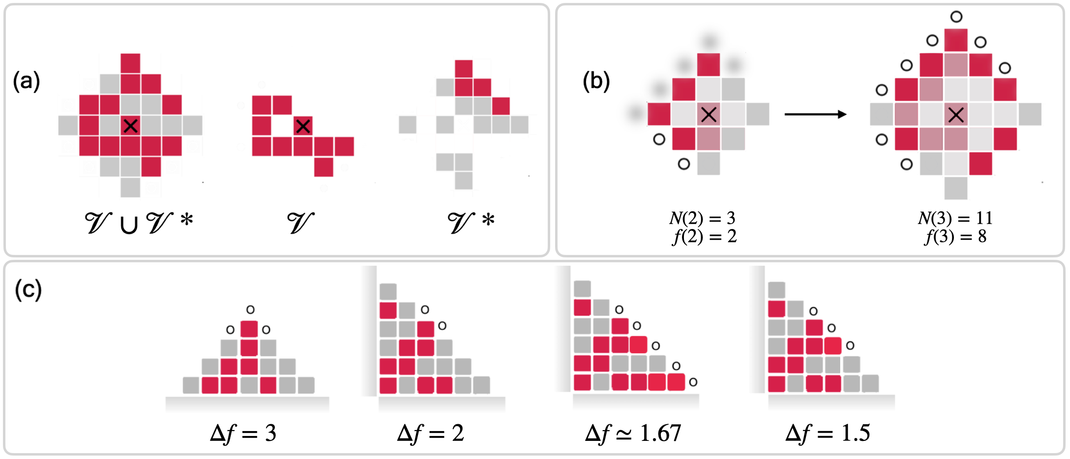
Figure 9: (a) An example of RGM growth after $t=3$ steps (leftmost part of the panel). For the sake of simplicity, neither blank nodes nor active frontier nodes are represented in the figure. In the middle of the panel, the seed cluster $\mathcal{V}$ marked with "$\times$" is shown. On the rightmost part of the panel we report the coloured nodes on the lattice that are not part of the seed cluster, namely the set $\mathcal{V*}$. (b) Two subsequent steps of a typical RGM realisation, respectively for $t=2$ (left) and $t=3$ (right). For the sake of simplicity, the blank nodes are not shown in the figure. The lighter tone represents the RGM cluster at the previous step. For both steps, $N$ and $f$ are shown. Nodes in $\mathcal{V*}$ that can potentially become part of $\mathcal{V}$ at the next step are coloured in blurred grey. (c) Different values of $\Delta f$ are associated with different sets of nodes in the seed cluster active frontier. In this picture, the shadowed stripes in each of the cases represent the bulk of $\mathcal{V}\cup\mathcal{V*}$. The highest value of $\Delta f$ is associated with the leftmost configuration.

We multiplied these contributions by $\Delta f(t+1)$, which is the expected increase in the size of $f(t+1)$ after the assignment of colours at $t$. $\Delta f(t)$ is defined as the ratio between the number of nodes in $\mathcal{V}$ sharing edges with the frontier at time $t$ and the number of nodes in $f(t)$: it describes the average potential increase in size due to each node in $\mathcal{V}$ that borders with the active frontier, from one growth step to the next (see Fig. 9(c)). We are now interested in solving these equations. For $t=0$ we have:

$$f(1)=p(c)[f(0)+f_{e}(0)]\Delta f(1)$$

And for $t=1$:

$$f(2)=p(c)[f(1)+f_{e}(1)]\Delta f(2)=$$

$$=p(c)^{2}[f(0)+f_{e}(0)]\Delta f(1)\Delta f(2)+p(c)f_{e}(1)\Delta f(2)=$$

$$=p(c)^{2}f(0)\Delta f(1)\Delta f(2)+p(c)^{2}f_{e}(0)\Delta f(1)\Delta f(2)+p(c)f_{e}(1)\Delta f(2)$$

So, solving the Eq. 11 for $f(t)$, we obtain:

$$f(t)=f(0)p(c)^{t}\prod_{j=1}^{t}\Delta f(j)+\sum_{j=0}^{t-1}\left[p(c)^{t-j}f_{e}(j)\prod_{l=j+1}^{t}\Delta f(l)\right]$$ (12)

Similarly, we can solve Eq. 11 for $N(t)$. For $t=0$ we have:

$$N(1)=N(0)+f(0)p(c)+N_{e}(0)$$

Then, for $t=1$:

$$N(2)=N(1)+f(1)p(c)+N_{e}(1)=$$

$$=N(0)+p(c)f(0)+N_{e}(0)+p(c)f(1)+N_{e}(1)=$$

$$=N(0)+N_{e}(0)+N_{e}(1)+p(c)[f(0)+f(1)]$$

And for $N(t)$:

$$N(t)=N(0)+\sum_{k=0}^{t}N_{e}(k)+p(c)\sum_{k=0}^{t}\left[f(0)p(c)^{k}\prod_{j=1}^{k}\Delta f(j)+\sum_{j=0}^{k-1}\left(p(c)^{k-j}f_{e}(j)\prod_{l=j+1}^{k}\Delta f(l)\right)\right]$$ (13)

where we have used Eq. 12 for $f(t)$.

We will now propose a mean-field approach for approximating the quantities $\Delta f(t)$ and $f_{e}(t)$ and obtaining an estimate for the observed $f(t)$ and $N(t)$. We performed $5\times 10^{6}$ simulations of RGM in the case $|C|=2$. We set the maximal growth steps, i.e. the growth step at which the process stops even if the cluster still has an active frontier, at $t=200$. We collect all the values of $\Delta f(t)$, $f_{e}(t)$ and $N_{e}(t)$ at each growth step $t$, and then we obtained $\overline{\Delta f}(t)$, $\overline{f_{e}}(t)$ and $\overline{N_{e}}(t)$ as the average over the number of different values of $\Delta f$, $f_{e}$ and $N_{e}$ at growth step $t$. We plug $\overline{\Delta f}(t)$ and $\overline{f_{e}}(t)$ in Eq. 12 to obtain our mean-field estimate for $f(t)$:

$$\overline{f}(t)^{est}=f(0)p(c)^{t}\prod_{j=1}^{t}\overline{\Delta f}(j)+\sum_{j=1}^{t-1}\left[p(c)^{t-j}\overline{f_{e}}(j)\prod_{l=j+1}^{t}\overline{\Delta f}(l)\right]$$ (14)

Notice that in Eq. 12, the sum starts from $j=0$, while in Eq. 14 from $j=1$. This is because, at each time step, the measured value of $\overline{f_{e}}(t)$ is nothing less than the fraction $p(c)$ of $f_{e}(t)$ nodes, so the exponent of $p(c)^{t-j}$ is reduced by one. Then, we collect all the observed values of $f(t)$ at each growth step $t$, and we obtain $\overline{f}(t)^{obs}$ as the averaged observed $f(t)$ over the total number of different values of $f(t)$ at $t$. The results are shown in Fig. 10(a).

Note that the mean-field theory replicates quite closely the observed trend for the active frontier, but it begins to deviate slightly after $t=40$. It diverges the most in the region between $t=[100,140]$, signalling that the model somehow cannot capture the trend for large $t$, where we have mostly fluctuations and contributions from explosive events, i.e. $t$ steps where the cluster has grown explosively thanks to contributions from $\mathcal{V*}$.

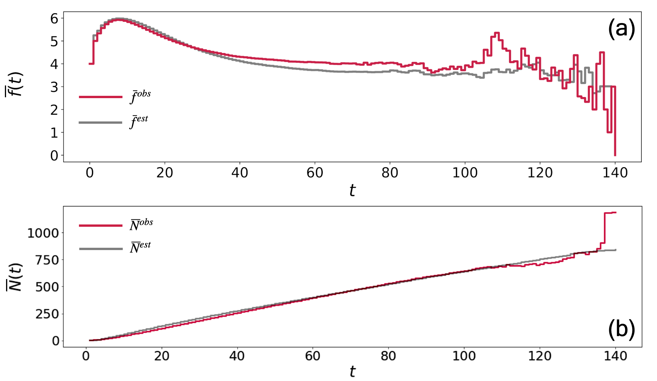
Figure 10: The observed active frontier $\overline{f}(t)^{obs}$ (a) and the observed size $\overline{N}(t)^{obs}$ (b) of RGM clusters are depicted with red solid lines. Each line is obtained from $5\times 10^{6}$ realisation. Estimated active frontier $\overline{f}(t)^{est}$ and estimated size $\overline{N}(t)^{est}$ are shown as dark grey solid lines. Notice the excellent agreement between the mean-field theory and the data.

This discrepancy is due to a variety of factors. First, $\Delta f$ is just an overall average value that is assumed equal for all the nodes of the frontier. Moreover, we implicitly assumed that $\Delta f$ is the same for nodes in $\mathcal{V}$ bordering the frontier, and nodes in $\mathcal{V*}$ bordering blank nodes in $\mathcal{G}$: this is also another approximation since we don’t know if the two contributions are different. However, the mean-field theory captures very well the behaviour of RGM for $t=[0,40]$. In the range $t=[40,100]$ the curve converges towards $f(t)=4$, and the mean-field curve follows this trend quite closely. After $t=100$, the mean-field can still provide a qualitative estimation of the data, despite the predominance of large fluctuations.

We adopt a similar mechanism to obtain our mean-field estimate for $N(t)$:

$$\overline{N}(t)^{est}=N(0)+\sum_{k=0}^{t}\overline{N_{e}}(k)+p(c)\sum_{k=0}^{t}\left[f(0)p(c)^{k}\prod_{j=1}^{k}\overline{\Delta f}(j)+\sum_{j=1}^{k-1}\left(p(c)^{k-j}\overline{f_{e}}(j)\prod_{l=j+1}^{k}\overline{\Delta f}(l)\right)\right]$$ (15)

Also in this case, we collect all the observed values of $N(t)$ at each growth step $t$, and we obtain $\overline{N}(t)^{obs}$ as the averaged observed $N(t)$ over the total number of different values of $N(t)$ at $t$. The results are shown in Fig. 10(b). More than in the case of $f(t)$, the model follows in a very good agreement the data curve for the size $N(t)$ in the whole observed range of growth steps. It deviates slightly after $t=100$, accordingly to what we found for the tail of the active frontier, where the fluctuations become predominant.

V.1 Mean-field active frontier for large N.

It is easy to use a mean-field argument to explain the observed value of the active frontier of RGM clusters when $N$ becomes large. By looking at Fig. 10(a), we can indeed notice that in the interval $t=[40,100]$ the value of $\overline{f}(t)^{obs}$ is flat and can be fitted very well by the line $\overline{f}(t)=4$. The trend diverges from the value $4$ only for $t>100$ when the fluctuations, due to a smaller number of points in the dataset, dominate the behaviour of the $\overline{f}(t)^{obs}$.

In Fig. 11(a) we show the probability distribution for $\Delta f$ for the value $t=75$ after $10^{7}$ RGM realisations: we choose this $t$ because it lies in the interval $t=[40,100]$ where $\overline{f}(t)^{obs}$ is flat. The distribution appears to be extremely heterogeneous, with some peaks that represent the more probable configuration of $\Delta f$. In the table in Fig. 11(a), we also collect the probability associated with the three most probable $\Delta f$, along with their value. The distribution remains very similar and stable for each $t$ in the range $t=[40,100]$, so we make the assumption that it has to describe the mean behaviour of $\Delta f$ when $N$ becomes large. In Fig. 11(b) we show a schematic representation of RGM clusters where we only take into consideration the nodes that are immediately adjacent to the active frontier of the cluster. We only show the combinations of active frontiers and nodes that are related to the three most probable $\Delta f$. We propose that the most probable configurations of active frontier and nodes are the ones highlighted in red in Fig. 11(b), drawing on the evidence that large RGM clusters are elongated and surface-like: groups of connected nodes with a single large active frontier are not so probable, while single or double nodes with small active frontiers are preferred. We use the probabilities in the table in Fig. 11(a) to weight each configuration, and we obtain a mean-field approximation for $\overline{f}(t)^{obs}$ as:

$$f^{MF}\simeq\frac{\frac{(2+4+6)\times 0.46}{3}+\frac{(3+6)\times 0.24}{2}+5\times 0.1}{0.46+0.24+0.1}\simeq 4.27$$ (16)

which is in a good agreement with the value $f(t)=4$ that we observe in the flat region of $\overline{f}(t)^{obs}$.

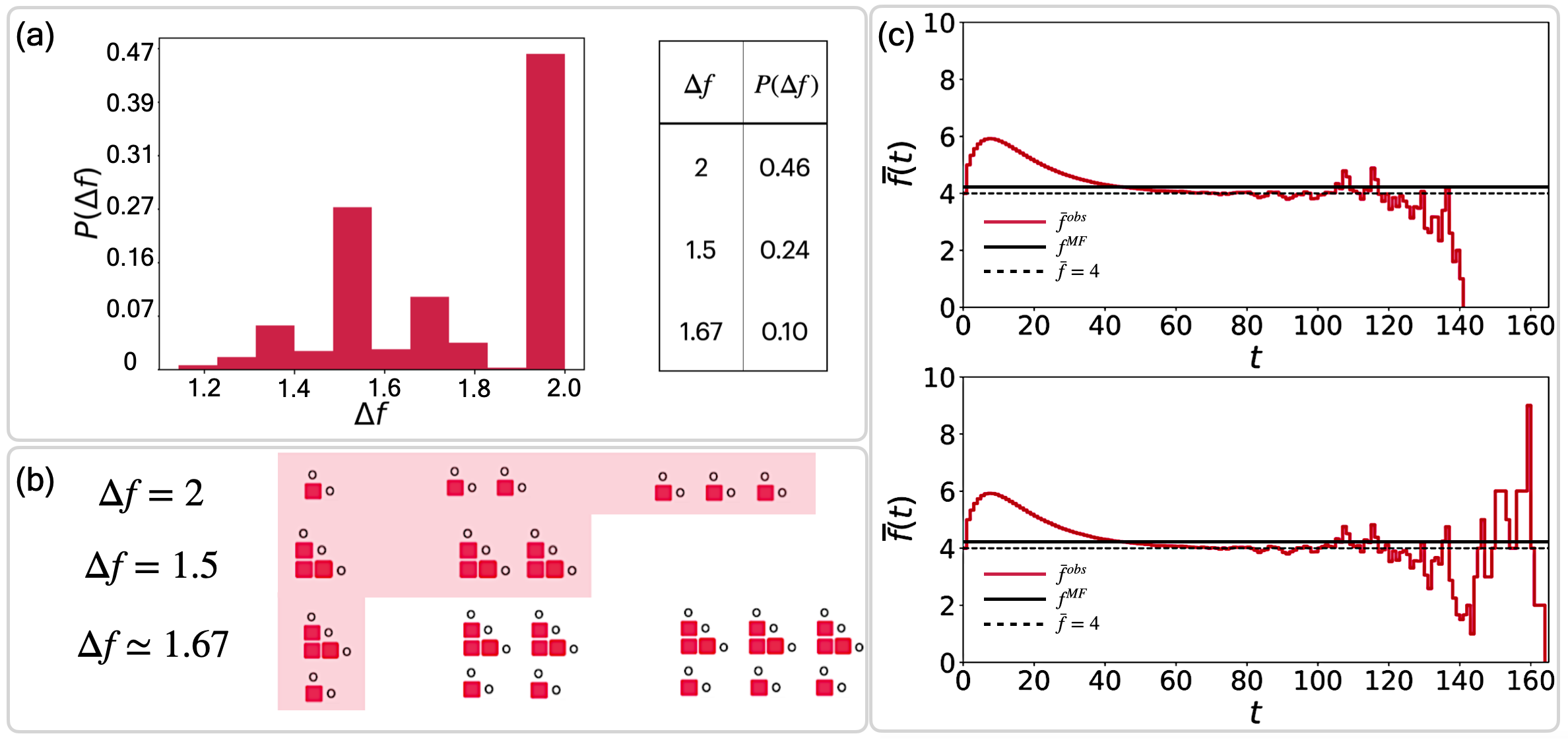
Figure 11: (a) The probability distribution for $\Delta f$ at $t=75$ after $10^{7}$ RGM realisations. The heterogeneous distribution (left) exhibits some peaks that represent the more probable configuration of $\Delta f$. Their probabilities are collected in the table (right). (b) A sketch of RGM clusters, where only nodes on the border of the cluster, along with their active frontier, are depicted. Each row is related to the respective $\Delta f$: for example, the first row is the collection of all the possible node-active frontier configurations that contribute to $\Delta f=2$. The proposed most probable configurations of active frontier and nodes are the ones highlighted in red. (c) The $\overline{f}(t)^{obs}$ trend for $9\times 10^{6}$ (top) and $10^{7}$ (bottom) realisations of RGM clusters. The observed curve is in red, while the mean-field approximation is depicted as a solid dark grey line. $\overline{f}(t)=4$ is shown as a dashed dark grey line.

In figure Fig. 11(c) we show the $\overline{f}(t)^{obs}$ trend for $9\times 10^{6}$ and $10^{7}$ realisations of RGM . In both plots, the $\overline{f}(t)^{obs}$ overlap quite well $\overline{f}(t)=4$ in the time range $t=[40,100]$. Furthermore, in the bottom plot the tail of the trend presents a huge fluctuation in the active frontier, with a maximal value of $\overline{f}^{obs}(157)=9$, followed by an abrupt transition to zero. This finding shows that the trend in the tail in Fig. 11(c) is only ephemeral, and the mean behaviour for the RGM active frontier has to be $\overline{f}(t)=4$.

VI Conclusions

Having a robust way of discriminating relevant patterns from trivial ones is of paramount importance in any field of research. But it is absolutely vital in the study of spatial complex systems, where the simple existence of spatial agglomerates of similar units has been far too often considered enough ground to conclude that some interesting behaviour is at work. By introducing the Uniform Random Colouring (URC) process as a random baseline for colouring lattices, we have shown that structures with considerable size can and will emerge, even in 2D square lattices, even in a random and uncorrelated process. This finding urges the use of caution when measuring quantities on real coloured spatial networks, as also very simple null models can generate large random structures, particularly when a small number of classes is available. We have shown that what makes clusters interesting (i.e., statistically significant), is not just their size, but a variety of geometric properties including their shape, tree-likeness, and surface. The mean exit time, i.e., the expected time needed for a uniform random walker to escape from the cluster, seems to be a promising candidate to summarise the geometric information about a cluster. The characterisation of shapes with minimal and maximal exit times, that we have proposed here, is just a first step in the exploration of this measure as an indicator of the compactness of a cluster configuration. Indeed, a spectral characterisation of cluster geometry might be possible, and could shed more light on the variety of interesting patterns we observe in real-world spatial systems. Overall, the results shown in this work provide a solid base upon which the significance of spatial clusters can be assessed. Given the importance of cluster analysis for a variety of spatial problems, from segregation to resource accessibility and distribution, the simple models and measures introduced in this work have a potentially wide applicability.

References

- (1) M. Barthelemy, Spatial networks. A Complete Introduction: From Graph Theory and Statistical Physics to Real-World Applications , Springer, 2022, ISBN: 978-3030941055
- (2) F. Papadimitriou, Spatial Complexity. Theory, Mathematical Methods and Applications, Springer Cham, 2020, ISBN: 978-3030596705
- (3) J. Rodríguez-Pérez, T. Wiegand and A. Traveset, Funct Ecol, 26, 1221-1229 (2012). Adult proximity and frugivore’s activity structure the spatial pattern in an endangered plant
- (4) R. Louf, M. Barthelemy, J. R. Soc. Interface, (2014). How congestion shapes cities: from mobility patterns to scaling
- (5) Bassel, G.W. and Stamm, P. and Mosca, G. and Barbier de Reuille, P. and Gibbs, D.J. and Winter, R. and Janka, A. and Holdsworth, M.J. and Smith, R.S. (2014). Mechanical Constraints Imposed by 3D Cellular Geometry and Arrangement Modulate Growth Patterns in the Arabidopsis Embryo
- (6) M. Batty, Cities and Complexity, MIT Press, Cambridge MA, 2005, ISBN: 978-0262524797
- (7) M. Batty, The New Science of Cities, MIT Press, Cambridge MA, 2013, ISBN: 978-0262318235
- (8) M. Barthelemy, The Structure and Dynamics of Cities, Cambridge University Press, Cambridge UK, 2017, ISBN: 978-1107109179
- (9) Bassolas, A., Sousa S., and Nicosia V. (2021). Diffusion segregation and the disproportionate incidence of COVID-19 in African American communities
- (10) Bassolas, A., Nicosia, V. (2021). First-passage times to quantify and compare structural correlations and heterogeneity in complex systems.
- (11) Haughey, M.J., Bassolas, A., Sousa, S., Baker, A., Graham, T. A., Nicosia, V., and Huang, W. (2023) First passage time analysis of spatial mutation patterns reveals sub-clonal evolutionary dynamics in colorectal cancer
- (12) Sousa, S., and Nicosia, V. (2022) Quantifying ethnic segregation in cities through random walks
- (13) Golomb, S. W. (1994) Polyominoes
- (14) Whittington, S. G. and Soteros, C. E. (1990) Lattice Animals: Rigorous Results and Wild Guesses
- (15) Xu, X., Wang, J., Zhou, Z., Garoni, T. M. and Deng, Y. (2014) Geometric structure of percolation clusters.
- (16) V. Latora, V. Nicosia, G. Russo, Complex Networks: Principles, Methods and Applications, Cambridge University Press, Cambridge UK, 2017, ISBN: 978-1108298681
- (17) Kawano M., Hotta C. (2019).Thermal Hall effect and topological edge states in a square-lattice antiferromagnet.
- (18) Grujić, J., Röhl, T., Semmann, D., Milinski, M., and Traulsen, A. (2012). Consistent strategy updating in spatial and non-spatial behavioral experiments does not promote cooperation in social networks.
- (19) Meakin P. (1986) A new model for biological pattern formation
- (20) Dill K. A., Bromberg S., Yue K., Fiebig K. M., Thomas D. P., and Chan H. S. (1995) Principles of protein folding: A perspective from simple exact models
- (21) Silva T. (2007) Animal enumerations on the 4,4 Euclidean tiling
- (22) Shirakawa T. (2012) Harmonic Magic Square, Enumeration of Polyominoes considering the symmetry
- (23) Mason J. (2023) Counting size 50 polyominoes
- (24) Cook H. (1970) Tree-likeness of dendroids and -dendroids
- (25) Potebnia A. (2018) New method for estimating the tree-likeness of graphs and its application for tracing the robustness of complex networks.
- (26) Trudeau, R. J. (1993) Introduction to Graph Theory
- (27) Barthelemy, M. (2017). Morphogenesis of Spatial Networks
- (28) Harris, C. C. (1964) A scientific method of districting.
- (29) Polsby, D. D. and Popper, R. D. (1991) The Third Criterion: Compactness as a procedural safeguard against partisan gerrymandering.
- (30) Li, W., Goodchild. M. and Church, R. L. (2022) An Efficient Measure of Compactness for 2D Shapes and its Application in Regionalization Problems.
- (31) Montero, R. S. and Bribiesca, E. (2020) State of the Art of Compactness and Circularity Measures
- (32) Wirth, M. A. (2020) Shape Analysis and Measurement
- (33) Kubale, M. (2004) Graph coloring
- (34) Behnamian, J. (2016) Graph colouring-based algorithm to parallel jobs scheduling on parallel factories.
- (35) Sudev, N., and Kok, J. (2020) On J-Colouring of Chithra Graphs
- (36) Eden, M., and Thevenaz, P. (1998). History of a stochastic growth model.
- (37) Sola, A., Turner, A. and Viklund, F. (2019) One-Dimensional Scaling Limits in a Planar Laplacian Random Growth Model.
- (38) Candia, J., and Albano, E. V. (2001). Comparative study of an Eden model for the irreversible growth of spins and the equilibrium Ising model.
- (39) Yu, J., Gang, H., and Ben-Kun, M. (1989). New growth model: The screened Eden model.
- (40) Damron, M. (2018) The size of the boundary in first-passage percolation.
- (41) James, H., Scogings, C. and Hawick, K. (2004). Parallel synchronization issues in simulating artificial life.
- (42) Frey, F., Bucher, D., Sochacki, K. A., Taraska, J. W., Boulant, S., and Schwarz, U. S. (2020). Eden growth models for flat clathrin lattices with vacancies.
- (43) Ivanenko, Y. V., Lebovka, N. I., and Vygornitskii, N. V. (1999). Eden growth model for aggregation of charged particles.
- (44) Agyingi, E., Wakabayashi, L., Wiandt, T., and Maggelakis, S. (2018) Eden model simulation of re-epithelialization and angiogenesis of an epidermal wound.
- (45) Manin, F., Roldán, É. and Schweinhart, B. (2023) Topology and Local Geometry of the Eden Model.
- (46) Teknomo, K., Gerilla, G., Hokao, K. and Benguigui, L. (2005) Unconstrained city development using the extension of stochastic Eden simulation.
- (47) Waclaw, B., Bozic, I., Pittman, M.E., Hruban, R.H., Vogelstein, B. and Nowak, M.A. (2015) A spatial model predicts that dispersal and cell turnover limit intratumour heterogeneity
- (48) Santalla, S. N. and Ferreira, S. C. (2018) Eden model with nonlocal growth rules and kinetic roughening in biological systems.
- (49) Newman, M. E. J. and Ziff, R. M. (2000) Efficient Monte Carlo Algorithm and High-Precision Results for Percolation.
- (50) Mertens, S. (2022) Exact site-percolation probability on the square lattice
- (51) Zierenberg, J., Fricke, N., Marenz, M., Spitzner, F. P., Blavatska, V. and Wolfhard, J. (2017) Percolation thresholds and fractal dimensions for square and cubic lattices with long-range correlated defects
- (52) Bernt, K. O. (2003) Stochastic Differential Equations: An Introduction with Applications.
- (53) Masuda, N., Porter, M. A., Lambiotte, R. (2017) Random walks and diffusion on networks
- (54) Bender, E. A., Williamson, S. G. (2010) Lists, Decisions and Graphs. With an Introduction to Probability.