Graph-Structured Kernel Design for Power Flow Learning using Gaussian Processes

Abstract

This paper presents a physics-inspired graph-structured kernel designed for power flow learning using Gaussian Process (GP). The kernel, named the vertex-degree kernel (VDK), relies on latent decomposition of voltage-injection relationship based on the network graph or topology. Notably, VDK design avoids the need to solve optimization problems for kernel search. To enhance efficiency, we also explore a graph-reduction approach to obtain a VDK representation with lesser terms. Additionally, we propose a novel network-swipe active learning scheme, which intelligently selects sequential training inputs to accelerate the learning of VDK. Leveraging the additive structure of VDK, the active learning algorithm performs a block-descent type procedure on GP’s predictive variance, serving as a proxy for information gain. Simulations demonstrate that the proposed VDK-GP achieves more than two fold sample complexity reduction, compared to full GP on medium scale 500-Bus and large scale 1354-Bus power systems. The network-swipe algorithm outperforms mean performance of 500 random trials on test predictions by two fold for medium-sized 500-Bus systems and best performance of 25 random trials for large-scale 1354-Bus systems by 10%. Moreover, we demonstrate that the proposed method’s performance for uncertainty quantification applications with distributionally shifted testing data sets.

I Introduction

The steady-state of a power grid is determined by solving a set of nonlinear equations, termed Alternating Current Power Flow (ACPF) that describe relation between nodal voltages (states) and input nodal power injections. These equations are non-linear and coupled, and do not come with analytical or closed-form expressions for nodal voltages as a function of the nodal injections. Instead, iterative methods like the Newton-Raphson load flow are employed for their solution. The challenge becomes even more pronounced when dealing with injection uncertainties in the system, as they can lead to significant fluctuations in the power flow. Frequently, the DC approximation is used to solve the ACPF with injection uncertainties. However, this approximation neglects the voltage information, which can lead to inaccurate results. The details of various methods can be found in [1]. Data-driven methods, particularly those based on linear approximations, have garnered considerable interest for power flow approximations [2, 3, 4]. Nevertheless, these linear models have limited capacity to capture the full non-linearity of power flow, and lifted approaches [5] tend to lose interpretability and require high sample complexity. Recently Deep Neural Networks (DNNs) have made significant advancements as universal function approximators with increased expressiveness, particularly via the idea of physics-informed machine learning [6]. This direction has also been explored for power flow learning [7, 8, 9]. Even though DNNs are powerful function approximators, they have limited interpretability, and obtaining confidence levels for their predictions is challenging. Without confidence information, using these predictions for critical system operations and planning in power systems, becomes difficult. Moreover, DNNs require an exponentially large number of samples to learn the power flow function. For instance, more than 10,000 training samples are used to learn voltage solutions for the 118-bus system in [7, 8, 9].

Gaussian process (GP) learning [10] is a versatile probabilistic method for function estimation. Compared to other approaches, such as DNNs, GP offers distinct advantages, particularly in terms of predictive uncertainty. Its non-parametric nature enables flexible representation of uncertainty, allowing for hyperparameter tuning and effective modeling even with limited data [10]. These characteristics make GP a powerful tool for capturing complex relationships in data while providing reliable predictions. In power systems, GP has been used for optimal power flow (OPF) learning [11, 12], system dynamics inference [13], stochastic OPF [12], stability margin prediction [14] and various other applications. In [15, 16, 17], GP is employed as a tool to approximate power flow. GP has been shown to be advantageous by providing differentiable non-linear closed-forms of power flow with predictive uncertainty, and interpretability [17]. One notable drawback common to all these GP works is their applicability primarily to small to medium-sized systems with a limited number of uncertain injections, such as 110 in the case of [17]. This scale limitation is because exact GP inference has cubic complexity with respect to number of samples [10] while number of samples required for learning increases rapidly with system size (or input dimensions). A possible way around of this problem is breaking the large dimensional input space into multiple spaces.

Additive GP is a modeling approach where multiple sub-kernels are defined to capture different aspects of the data [18, 19]. Each sub-kernel operates on a specific subset of input variables or features, and their combination yields the final kernel, allowing for a fast and flexible representation of the data. In [20], authors apply this idea of additive GP to improve the learning performance for probabilistic power flow. The kernel design problem is formulated as a bi-level optimization problem, which is NP-hard in nature. This makes kernel design expensive and requires to conduct kernel search among $2^{\text{order}}$ unique kernel combinations (where order is maximum number of sub-kernels used together in additive fashion).

Another approach for low sample complexity learning is active learning (AL) [21]. The idea is to sample training points successively such that next training point contains maximum information about the unknown target function [22]. The theory and analogy directly follows Bayesian optimization (BO) [23]. GP is very well suited as a surrogate, in the absence of true target function, for information maximization [24]. However, AL (and BO) suffers from curse-of-dimensionality as search space grows exponentially with dimensions of input, which is the number of injections. Standard GP [17] and higher-order additive kernel GP [20] are hence not suitable for AL. Based on aforementioned limitations, it is clear that for large-scale power flow approximations, we require a kernel design that can be expressed using lower-dimensional input sets, exhibits lower sample complexity, and yet captures the correlated injection effects. Additionally, the Kernel design step must not require solving a difficult optimization problem at each step, reducing overall learning complexity. Further, the kernel design should allow for bypassing the curse-of-dimensionality in the information maximization problem, when used with Active Learning (AL).

In this paper, we propose Vertex-Degree Kernel (VDK), a graph-structured design that effectively learns the voltage-injection function in large-scale systems. VDK embeds network topology information into a Gaussian process (GP) model using a neighborhood-aggregation strategy and breaking the function into lower-dimensional latent functions. Additionally, we introduce a reduced VDK representation that enhances computational efficiency without compromising performance. Importantly, the design of VDK and its reduction strategy does not necessitate solving hard optimization problems, and uses the training dataset only for parameter estimation. As a result, the proposed VDK-GP framework avoids a large time or sample burden on the learning method. Unlike standard physics-informed learning approaches [25], our approach’s reliance on grid structure, provides an alternative way to incorporate physics into the learning model. We use maximum log-likelihood with closed-form to optimize kernel hyper-parameters (chapter 2 [10]). Moreover, we devise a novel network-swipe active learning (AL) algorithm that intelligently selects training points to maximize information gain– without relying on labeled power flow data. The proposed AL method requires large instances of function evaluation instead of solving multitude of power flows. Thus, our AL algorithm enhances model performance in terms of both speed and generalization. Further, the proposed network-swipe AL eliminates the need to solve complicated information gain maximization problems for additive GP models with overlapping variables [26, 27]. To assess the effectiveness of our proposed approaches, we conduct benchmark experiments on medium to large-sized power networks, taking into account uncertain injections at all load buses.

The main contributions of this study can be delineated as:

• Development of a graph-structured kernel, the vertex-degree kernel (VDK), for effectively learning the voltage-injection function in large-scale power systems. VDK leverages a neighborhood-aggregation strategy to incorporate network graph information into a Gaussian process (GP) model. Additionally, a reduced VDK representation is introduced, reducing the number of sub-kernels for faster implementation without compromising performance.

• A novel network-swipe active learning (AL) algorithm that intelligently selects training points to maximize information gain without relying on labeled data, eliminating the need for solving numerous power flows for training data collection. The proposed network-swipe AL shows more than 1.5 fold improvement for 118-Bus system and two fold improvement for 500-Bus system over VDK-GP with same training dataset.

• Benchmarking the proposed VDK-GP and network-swipe AL for medium to large size power networks while considering all load buses having uncertain injections. Using only 100 training samples, the proposed method achieves mean absolute errors (MAEs) of the order of $10^{-4}$. Results show 3-5 fold reduction in sample complexity compared to full GP. The proposed voltage-injection function is also utilized to perform uncertainty quantification (UQ) in non-parametric i.e. distribution agnostic settings.

The remainder of this paper is organized as follows. In Section II, we provide a brief overview of the power flow learning and we present the proposed VDK-GP and reduced representation of VDK. In Section III, we describe the idea of information gain, outline challenges in designing AL methods and the proposed network-swipe AL algorithm. In Section IV, we present the results for benchmark experiments and uncertainty quantification for medium to large systems and discuss insights. Finally, in Section V, we conclude the paper and discuss future work.

II Vertex Degree Kernel for Power Flow

We begin this section by reviewing power flow in functional form (from GP learning point of view) and then describe the limitations of standard kernel architectures and of simple additive kernel. Later this section presents the proposed graph-structured kernel design along with physical intuition and mathematical details of the same. Both ‘bus’ and ‘node’ are used to indicate power network vertex. Complex voltage at a node is $v_{j}=V_{j}\angle{\theta_{j}}$ with $V_{j}$ as magnitude and $\theta_{j}$ as the phase angle. Load and injection both are used in their net-form i.e. demand-generation = load while generation - demand = injection, and they refer to complex power $s_{j}=[p_{j};q_{j}]$. Here, $p_{j}$ ($q_{j}$) is real (reactive) load/injection at $j$-th node. All buses of the network are collected in set $\mathcal{B}$ with $|\mathcal{B}|$ representing set length i.e. the number of nodes. The set of network graph vertices (nodes) is denoted by $\mathcal{V}$, and the set of network edges (branches) is denoted by $\mathcal{E}$. Further, power flow, as a mapping between node voltage and injection vector, in a functional form can be represented as [17]

$$V_{j}(\mathbf{s})=f_{j}(\mathbf{s})+\varepsilon$$ (1)

where, $V_{j}(\mathbf{s})$ is $j-$th node voltage measurement for injection vector $\mathbf{s}$ and $f_{j}(\mathbf{s})$ being unknown underlying function with $\varepsilon\sim\mathcal{N}(0,\sigma^{2}_{n})$ being i.i.d. Gaussian noise.

Now, we use GP to model an underlying node voltage function $f(\mathbf{s})$ (subscript $j$ is omitted for brevity). In GP we consider that function $f$ belongs to a zero mean Gaussian distribution [10] i.e.

$$f(\mathbf{s})\sim\mathcal{GP}\Big{(}\mathbf{0},K(S,S)\Big{)}$$ (2)

with $K(\cdot,\cdot)$ defining the covariance matrix or kernel matrix over the training samples and $S=[\mathbf{s}^{1}\dots\mathbf{s}^{i}\dots\mathbf{s}^{N}]$ being design matrix having $N$ injection vector samples from training set $\{\mathbf{s}^{i},V^{i}\}^{N}_{i=1}$. The kernel matrix $K$ is constructed using covariance or kernel function working over the injection vector i.e. an $i,j$-th element $K_{i,j}=k(\mathbf{s}^{i},\mathbf{s}^{j})$, (see [10, 17] for details). The kernel function works over injection vectors and have parameters termed as hyper-parameters $\boldsymbol{\rm\theta}$. These hyper-parameters can be learned using maximum log-likelihood estimation (MLE) for exact inference [10]. Upon learning, the GP provides mean and variance predictions of the function as

$$\mathbb{E}[f(\mathbf{s})] =\mu_{f}(\mathbf{s})=\mathbf{k}^{T}\big{[}K+\sigma^{2}_{n}I\big{]}^{-1}\mathbf{{V}}$$ (3)

$$\mathbb{V}[f(\mathbf{s})] =\sigma^{2}_{f}(\mathbf{s})=k(\mathbf{s},\mathbf{s})-\mathbf{k}^{T}[K+\sigma^{2}_{\epsilon}I]^{-1}\mathbf{k}$$ (4)

here, upon learning, $K=K(S,S)$ refers to the kernel matrix with a $\boldsymbol{\rm\theta}$ vector and $\mathbf{k}=[k(\mathbf{s}^{1},\mathbf{s})\dots k(\mathbf{x}^{N},\mathbf{x})]$ is a vector obtained by applying kernel function over $\mathbf{s}$ and each training sample in $S$. Also, $\mathbf{V}$ is measured target node voltage vector. This implies that GP model not only provides point prediction as $\mu_{f}(\mathbf{s})$ Eq. (3) but also gives confidence level via predictive variance $\sigma^{2}_{f}(\mathbf{s})$. The simplest interpretation of this confidence is that there is 95% chance that a true voltage solution obtained via power flow solving, at a given injection, will be within $\mu_{f}(\mathbf{s})\pm 2\sigma_{f}(\mathbf{s})$. This means, lower value of $\sigma^{2}_{f}(\mathbf{s})$ implies a higher confidence GP model for power flow.

The ability of GP to fit a voltage function directly depends upon the selection of the kernel function which constructs the covariance matrix. This kernel construction allows us to infuse our prior understanding about voltage function into the learning models. By constraining the injection space to the feasible power flow region, we understand that voltage is a smooth function of injections. Therefore, smooth kernels such as square exponential kernel, is extensively used for power flow learning [20, 17, 15, 16]. It is important to note that using a kernel function $k:\mathbb{R}^{2|\mathcal{B}|}\rightarrow\mathbb{R}$ will imply that GP learning via log-likelihood maximization is done over a $2|\mathcal{B}|$ dimensional injection space. Although, [20] works with one dimensional sub-kernel ($k_{r}$ in equation (3) of [20]), the effective kernel dimension is much larger [20].Note that the additive GP idea considers that a high-dimensional function can be partitioned in low-dimensional sub-functions [18]. However, a simple additive kernel, with each sub-kernel only working with one node’s injection input $\mathbf{s}_{i}$, will ignore the injection correlation on voltage. By observing the power flow equations, we know that such correlations exist via admittance matrix and quadratic voltage multiplication terms in power flow [28]. Authors in [20] attempted to solve this issue by searching a kernel among higher-order kernels, making kernel design expensive. Thus, our objective of kernel design is to design an additive kernel using i) sub-kernels working over a small subset of injection vector, ii) capture injection correlation effect on voltage, and iii) determine its structure without solving a large optimization problem.

II-A Proposed Kernel Design

We propose to exploit the network graph structure to design an additive kernel by utilizing nodal sub-kernels that focus on neighborhood injections. The physical intuition behind the proposed kernel design is that a node voltage is affected by all node injections but injection correlation effect is limited to the neighborhood effects. The injection correlation effect can be defined as change in voltage due to simultaneous change in two or more nodal injections. If there is no injection correlation effect, than a node voltage will not be affected by simultaneous change any more than individual change effect. In other words, interaction between two far away nodes can be neglected in terms of their effect on voltage. Note that this idea does not ignore the effect of any node injection, but only omits the correlated effect of non-neighbor node injections. For a node $j$, we define neighborhood as all nodes connected directly to node $j$ and the neighborhood injection variable set is $\{\mathbf{x}_{j}=\{\mathbf{s}_{i}|(i,j)\in\mathcal{E}\}$. Therefore, each nodal sub-kernel, called Node Neighborhood Kernel (NNK) hereafter, takes only a few node injections as inputs. This means the dimensionality of the learning space for each kernel is equal to its vertex degree plus one. The complete additive kernel, the sum of these NNKs, is termed as vertex degree kernel (VDK) and is defined as

$$k_{v}(\mathbf{s}^{i},\mathbf{s}^{j})=\sum^{|\mathcal{B}|}_{b=1}k_{b}(\mathbf{x}^{i}_{b},\mathbf{x}^{j}_{b})$$ (5)

here, $k_{b}(\mathbf{x}^{i}_{b},\mathbf{x}^{j}_{b})$ is the NNK working over $\mathbf{x}_{b}\subset\mathbf{s}$ and total number of sub-kernels is equal to the number of nodes in the network. Each sub-kernel $k_{b}(\cdot,\cdot)$ has hyper-parameters $\boldsymbol{\rm\theta}_{b}$ and combined hyper-parameter vector is $\boldsymbol{\theta}=[\boldsymbol{\rm\theta}_{1},\cdots,\boldsymbol{\rm\theta}_{|\mathcal{B}|}]$. As the sum of valid kernel function is a kernel function, standard exact inference can be performed via optimizing MLE using $k_{v}(\cdot,\cdot)$ as long as each NNK is a valid kernel [19, 18, 10]. Fig. 1 shows the idea of NNK construction using a part of 118-Bus system. Each node has one NNK where real and reactive power injections of that node and its neighborhood nodes are considered as input. Main properties of VDK (5) are

• Dimension Reduction: As VDK is an additive function, the effect of the input dimensionality will directly depend on the largest sub-kernel input dimension $\max_{b}|\mathbf{x}_{b}|$ which is equal to the maximum vertex degree plus one. Clearly, the largest vertex degree is much smaller than the number of nodes in the network, thus reducing the effective kernel dimensions. This will lead to significant sample complexity reduction.

• Neighborhood Correlation Effect Consideration: In contrast to a simple additive kernel, the proposed VDK considers the correlated effect of neighborhood injections using NNK as shown in Fig. 1. This design is based on the intuition that correlated injection effects are significantly reduced as the distance between nodes on the network graph increases. Notably, all node injections appear in at least two NNKs, and hyperparameters $\boldsymbol{\theta}$ are optimized via MLE using the complete VDK. Therefore, VDK effectively captures injection correlation effects beyond the immediate neighborhood.

• Constant Kernel Structure: The proposed VDK design exploits the graph structure and remains unchanged unless the graph-structure or admittance matrix itself changes. This eliminates the need to solve any optimization problem for obtaining kernel structure. Moreover, being inspired by network graph, proposed VDK is equivalent to infusing the physical system information into the machine learning model, thus introducing a novel approach to the thriving research field of physics-informed machine learning [6].

The aforementioned features clearly highlight that the proposed VDK design achieves all three objectives laid down for the kernel design in this work. An important point is that VDK design can work with any sub-kernel as long as NNK is a valid kernel. Considering smoothness of $f(\cdot)$, and the power flow learning methods [17, 20], we opt for square exponential kernel as NNK.

Remark 1.

The features indicated above are to highlight the additional benefits of using the proposed VDK instead of full kernel in GP modeling of ACPF. The proposed VDK-GP also possess all the advantages of standard GP model. The proposed VDK-GP based ACPF model also provides closed-form, is interpretable, provides a subspace-wise approximation and is robust against input distribution changes since it is a non-parametric method. See [17] for detailed discussion on properties and advantages of GP-based ACPF approximation.

Notice that from Eq. (5), it is clear that the total number of sub-kernels required for a given system is equal to the number of nodes in that system. This implies a hyperparameter search space twice the size of the network and overlapping input sets for NNKs. Here, we propose a straightforward approach to address these challenges.

Figure 1: A part of 118-Bus system showing the idea of vertex degree kernel construction via working over injections of a given nodes and its immediate neighbors. In Eq. (5), we use $\mathbf{x}_{b}$ to represents all the injection variables in $b$-th NNK as $k_{1}(\mathbf{x}_{1},\cdot)=k_{1}(\mathbf{s}_{1},\mathbf{s}_{2},\mathbf{s}_{3},\cdot)$. For brevity, second input element in kernel function is represented using $(\cdot)$.

II-B Reduced VDK Representation

Consider a situation where set of neighborhood injection for a given node is a proper subset of another node’s neighborhood injection set i.e. $\mathbf{x}_{i}\subsetneq\mathbf{x}_{j}$. In such a situation, $i$-th NNK in Eq. (5) can be considered redundant as $k_{i}$’s all inputs are already present in $k_{j}$’s input set. We propose a reduced VDK representation by removing all such redundant kernels.

Fig. 2 presents two topological designs in typical power networks where $\mathbf{x}_{i}\subsetneq\mathbf{x}_{j}$. First, it is straightforward to see that a leaf node always has a proper subset injection set, as shown in 2. Another condition is when a sub-graph is connected in a triangle shape and at least one node of it is not connected to any other node, outside this triangle. Note that as the graph structure is fixed, and the NNKs are constant, the process of obtaining redundant sub-kernels involves a straightforward comparison and analysis of the kernel vectors. By matching and analyzing the kernel vectors, we can easily identify and remove redundant sub-kernels from VDK. There is no involvement of optimization or combinatorial problems in this reduction approach. Table I shows the reduced VDK size and percentage reduction. As the network size increases, this approach helps in reducing the hyper-parameter space dimension, leading to potential improvements in learning performance and implementation time. Importantly, this reduction method preserves VDK structure’s neighborhood correlation effect consideration.

Figure 2: Idea of VDK reduction by removing proper subset NNKs.

TABLE I: Size Reduction via Reduced VDK Representation

System Size†	Reduced VDK Size	Reduction
118-Bus	97	17.7%
500-Bus	238	52.4%
1354-Bus	786	41.9%
† VDK size in Eq. (5) is equal to system size i.e. $|\mathcal{B}|$

Since, the proposed VDK overcomes the the constraints imposed by high-dimensionality of the input space, it allows for the design of designing active learning (AL) mechanism to find training samples successively. Below we present an AL method designed for VDK-GP based power flow learning.

III Active Learning Mechanism

The power flow learning quality will be directly affected by the function information available in training set. Also, we are interested in knowing: How to learn $f(\mathbf{s})$ rapidly? For this, training sample set must be selected to maximize the information about the original function, and such a learning mechanism is called active learning (AL) [21]. AL is a technique that reduces sample complexity by intelligently selecting informative instances for labeling. It leverages unlabeled data (only injection inputs) to guide the learning process, allowing the model to focus on areas of uncertainty and ambiguity. By actively choosing the most valuable samples to label (to solve power flow), AL significantly reduces the time burden while maintaining or even improving the model’s performance.

In GP modeling (or Bayesian setting in general) ‘information gain’ is used as a measure to quantify the informativeness of a training set or sample. Let, $\mathcal{A}\subset\mathcal{L}$ where $\mathcal{L}$ is the complete training set or space then information gained by samples in $\mathcal{A}$ is mutual information between voltage function $f$ and $\mathbf{V}_{\mathcal{A}}$, which is a vector of voltage samples following Eq. (1)) [24]. Considering the GP model Eq. (2) and i.i.d. Gaussian noise $\varepsilon$, this information gain can be expressed as $I(\mathbf{V}_{\mathcal{A}};f)=(1/2)\log|I+\sigma^{-2}_{\epsilon}K_{\mathcal{A}}|$, where $K_{\mathcal{A}}$ is kernel matrix constructed using input samples in set $\mathcal{A}$ [24]. Importantly, finding $\mathcal{A}\subset\mathcal{L}$, where training samples are limited by a number $N$ ($|\mathcal{A}|\leq N$), by optimizing $I(\mathbf{V}_{\mathcal{A}};f)$ is an NP-hard problem [24]. However, two results facilitate tractable AL via information gain in GP learning. First, in [29] information gain has shown to be having submodularity property, which means that greedy algorithm provides guaranteed performance. Second, the information gain by a new sample can be expressed in terms of the predictive variances Eq. (4), using existing model [24]. By combining the submodularity property and variance-information gain equivalence, next training sample can be obtained by solving

$$\mathbf{s}^{t+1}=\operatorname*{arg\,max}_{\mathbf{s}\in\mathcal{L}}\,\sigma^{t}_{f}(\mathbf{s})$$ (6)

here, $\sigma^{t}_{f}(\cdot)$ is predictive standard deviation after training using $t$ samples. As eluded in the introduction, search space $\mathcal{L}$ increases with system size and the non-convex function makes Eq. (6) quickly intractable for standard GP [17], having input vector of size ${2|\mathcal{B}|}$ in kernels [23]. In standard additive GP setting, the information gain Eq. (6) objective (with mean term if Bayesian optimization (BO) problem is being solved) is completely separable in terms of lower-dimensional sub-kernels, reducing AL simply to a parallelizable set of small dimensional optimization problems [30]. However, the proposed VDK (both complete and reduced form Fig. 1 and Fig. 2) has overlapping input groups i.e. $\mathbf{x}_{i}\cap\mathbf{x}_{j}\neq\emptyset\,\forall i,j$. Therefore, direct split approach of [30] is not applicable. Methods such as [26, 27] propose BO (covering AL) with overlapping groups in additive GP. However they either require to construct specialized dependency graphs or rely on randomization. Use of these approaches for AL will take away the constant interpretable structure feature of the proposed VDK.

We propose a block-descend type algorithm to work over the concept of network-swipe and exploit VDK design for optimization of Eq. (6). Intuitively, power flow physics suggests that relative impact (or sensitivity) of $j$-th node injection change on $j$-th node voltage change will be high and this impact tend to reduces as we move away from the $j$-th node. Although, this relative impact is not linear or directly quantifiable, it suggests that a network-swipe structure of block-descend optimization can help in solving the high-dimensional AL problem Eq. (6) with the proposed VDK (5).The proposed network-swipe algorithm starts by solving Eq. (6) with respect to the $\mathbf{x}_{j}$, while keeping all other injections fixed, to learn $V_{j}(\cdot)$. It then proceeds to solve Eq. (6) for the next set of variables that serve as inputs for the neighborhood kernels of $k_{j}(\cdot,\cdot)$, excluding those already present in $\mathbf{x}_{j}$, while again keeping all other injections constant. This process is repeated iteratively, covering the entire network depth, until convergence is achieved. A graphical representation of the network-swipe algorithm is shown in Fig. 3 and now below present this idea in detail.

Figure 3: Idea of network-swipe algorithm for AL. At each depth or layer, only unique elements which are not covered already in any prior layer are treated as variables for information maximization. Note that in second layer, updated first layer inputs $\widehat{\mathbf{x}}^{t+1}_{\mathcal{D}_{1}}$ are used along with last swipe inputs of all other node injections $\widehat{\mathbf{x}}^{t}_{\mathcal{D}_{3\dots d}}$, as given in Eq. (7).

Let, a re-oriented node indexing set, different for each target node, is $\mathcal{D}=\{\mathcal{D}_{1}\dots\mathcal{D}_{d}\}$ where subscript indicate depth or layer, from the target node point-of-view, where each node of the network is part of only one depth element $\mathcal{D}_{i}$. We abuse notations by using $\mathcal{D}$ to indicate layer set for an arbitrary target node voltage learning. Also, $\mathcal{D}_{1}$ will always only have target node into it i.e. $\mathcal{D}_{1}=\{j\}$ for $V_{j}(\cdot)$ learning. The second layer set $\mathcal{D}_{2}$ will consist of neighborhood nodes of $j$ and then $\mathcal{D}_{3}$ will have neighborhood nodes of $\mathcal{D}_{2}$ entries. Further, $\overline{\mathbf{x}}_{\mathcal{D}_{i}}$ represent set of unique node injections at depth $i$ of the network like in Fig. 1, $\overline{\mathbf{x}}_{\mathcal{D}_{2}}=\{\mathbf{s}_{1},\mathbf{s}_{2},\mathbf{s}_{3},\mathbf{s}_{5},\mathbf{s}_{12}\}$. Now, consider learning a $j$-th node voltage, than a single network-swipe is performed by solving following non-linear optimization problem sequentially for $i=1\dots d$

$$\widehat{\mathbf{x}}^{t+1}_{\mathcal{D}_{i}} =\operatorname*{arg\,max}_{\widehat{\mathbf{x}}_{\mathcal{D}_{i}}\in\mathcal{L}_{i}}\,\sigma^{t}_{f}(\widehat{\mathbf{x}}^{t+1}_{\mathcal{D}_{1\dots i-1}},\widehat{\mathbf{x}}_{\mathcal{D}_{i}},\widehat{\mathbf{x}}^{t}_{\mathcal{D}_{i+1\dots d}})$$ (7)

here, $\widehat{\mathbf{x}}_{\mathcal{D}_{i}}=\{\mathbf{s}_{j}|\mathbf{s}_{j}\in\overline{\mathbf{x}}_{\mathcal{D}_{i}}\,\text{and}\,\,\mathbf{s}_{j}\notin\overline{\mathbf{x}}_{\mathcal{D}_{i}}\forall\,j<i\}$ represents unique node injection variable at depth $j$ which are not present in any depth variable set lower than $j$ i.e. $\widehat{\mathbf{x}}_{\mathcal{D}_{3}}=\{\mathbf{s}_{4},\mathbf{s}_{6},\mathbf{s}_{8},\mathbf{s}_{11},\mathbf{s}_{16},\mathbf{s}_{117}\}$. The sub-script in $\widehat{\mathbf{x}}^{t}_{\mathcal{D}_{i+1\dots d}}$ indicates the collection of $\widehat{\mathbf{x}}_{\mathcal{D}}$’s. Also, $\mathcal{L}_{i}$ represents the hyper-cube slice with respect to injections present in $\widehat{\mathbf{x}}_{\mathcal{D}_{i}}$ and $\widehat{\mathbf{x}}^{t}_{\mathcal{D}_{i}}$ is the optimal value of variable with $(\cdot)^{t}$ indicated swipe index. A detailed explanation of single network-swipe is given in Fig. 3 while complete algorithm considering is given below.

Algorithm 1 Network-Swipe Algorithm for AL

1:$T$, $\mathcal{D}$, $\{\mathbf{s}^{1},V^{1}\}$

2:Initialize GP model (2) with VDK (5)

3:for $t=1$ to $T$ do

4:     Solve (7) for $\widehat{\mathbf{x}}^{t+1}_{\mathcal{D}_{i}}$, sequentially for $i=1\dots d$

5:     Solve ACPF for load $\mathbf{s}^{t+1}$ to get $V^{t+1}$

6:     Update GP model with $(\mathbf{s}^{t+1},V^{t+1})$

7:end for

8:Compute $\mu_{f}(\mathbf{s}),\sigma_{f}^{2}(\mathbf{s})$ for final GP

In Algorithm 1, with sample budget $T$, re-oriented node indexing set $\mathcal{D}$, consider the initial training dataset $\{\mathbf{s}^{1},V^{1}\}$ are input. Note that node index is omitted from both $\mathcal{D}$ and $V$ for brevity. Moreover, the step 3 in Algorithm 1 is for one network-swipe. Multiple swipes can be performed across network to improve the information gain. Further, for solving Eq. (7), in Algorithm 1 we use numerical optimization with different batch sizes. The use of numerical optimization over analytical is preferred to evaluate effect of ‘batch size’ which will directly benefit in extending the proposed network-swipe method to Batch Bayesian optimization [32]. Also, note that each layer can still have significantly large number of variables (e.g. 1354-Bus system has 216 kernels in one layer). The numerical optimization will allow to build parallelizable optimization methods, helping to scale and improve performance of the proposed network-swipe AL in future works.

IV Results and Discussion

This section presents the performance results of the proposed VDK-GP compared to standard full kernel GP. We work with the budget of 100 training samples for the proposed VDK-GP for all the networks. All testing is done on 1000 out-of-sample data points unless stated otherwise. We use powermodels.jl, for running power flow with default ACPF setting for data collection. Both training and testing datasets is sampled uniformly (unless stated otherwise) from injection hypercube, constructed around base-load point, in the given dataset. A $\pm 10\%$ hypercube means that all node injections/loads (both real and reactive power) lie between $0.9-1.1$ times of base value. We also present the application of the proposed VDK-GP models for uncertainty quantification (UQ) and show the distributional robustness of the proposed functional approximation of power flow. We use the Square Exponential Kernel for all simulations, both as full kernel and NNKs. All models are implemented in Julia using the ADAgrad solver and Zygote for auto-differentiation. Below, we benchmark the proposed method against the standard GP of full-dimensional kernel (Full GP hereafter). Later we elaborate the model performance gains attained through AL. Finally, UQ results– focusing on distributional robustness of the proposed power flow model are discussed. Two different error indicators are used for benchmarking– mean absolute error (MAE), and maximum error (ME)

MAE $$=\frac{1}{M}\sum_{i=1}^{M}\Big{|}\mu(\mathbf{s}^{i})-V(\mathbf{s}^{i})\Big{|}$$ (8)

ME $$=\max_{i}\Big{|}\mu(\mathbf{s}^{i})-V(\mathbf{s}^{i})\Big{|}$$

where $\mu(\mathbf{s}^{i})$ is mean voltage prediction of that particular node voltage, $V(\mathbf{s}^{i})$ represents the true values obtained by solving ACPF and $M$ is number of testing samples (1000 here).

IV-A Benchmarking

We begin by discussing the results on the 118-Bus system obtained from the pglib-library[33]. Fig. 4 shows the comparative performance of proposed VDK method against full GP for 500 random training-testing trials using 100 training and 100 testing samples as violin plots. It is evident from the left sub-figure that the proposed method outperforms the full GP in over 70% of instances in terms of per unit (pu) MAE. The right sub-figure shows maximum predictive variance(MPV) for each trial. The performance of the proposed method is evident in its ability to achieve a low predictive variance, indicating a high-confidence power flow model. This performance can be explained by understanding that the GP model (2), effectively fits a covariance function (with the kernel being the parameterized form of the covariance) to the available data. Consequently, when the training data is limited, a lower-dimensional covariance can provide a better fit compared to a higher-dimensional covariance. As a result, the neighborhood aggregation approach employed in designing the NNKs and VDK leads to a robust power flow approximation, enhancing confidence in the model’s accuracy. Fig. 5 shows absolute error values in pu for learning all node voltages using the same 100 training and 1000 testing samples. It is clear that proposed method has been able to achieve accuracy of same level for all node voltages. The approximation quality can be further improved by increasing the number of samples for voltages where the error is higher than the desired level.

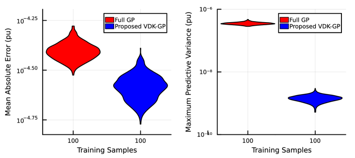
Figure 4: Performance of the proposed VDK-GP compared with full GP for learning $V_{1}$ with $\pm 10\%$ hypercube in 118-Bus system. Violins are made up of 500 random trial results, both sub-figures have y-axis in log-scale and 1000 points used in out-of-sample test (per trial).

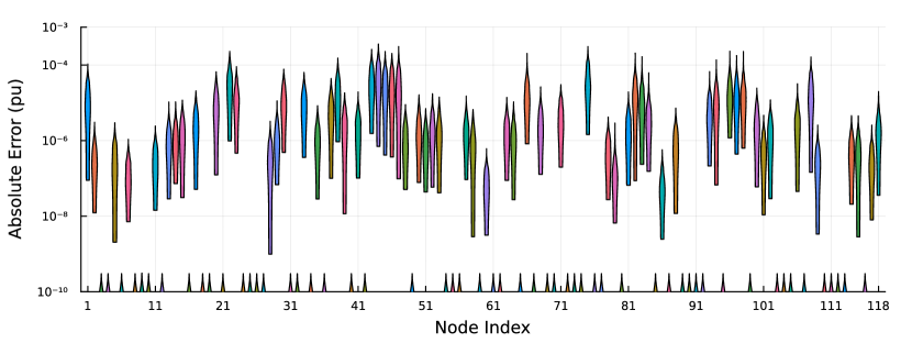
Figure 5: A random trial performance of the proposed VDK-GP, for all voltages of 118-Bus system within $\pm 10\%$ hypercube of uncertainty. Same 100 training and 1000 testing samples are used for all voltages. Small ticks near x-axis are of PV nodes i.e. constant voltage magnitude and y-axis is in log-scale.

We also tested the proposed method on a 500-Bus system from [33]. Fig. 6 shows a comparison between the Full GP and proposed VDK-GP performance based on 500 random trials. The left sub-figure shows a three-fold reduction in sample complexity of power flow learning using the proposed VDK-GP, while achieving the same MAE. Additionally, the MPV performance follows the same trend in the right sub-figure, where the proposed method results in a high-confidence (low MPV) power flow model due to its neighborhood aggregation strategy. As expected, the MAE values for 500-Bus system are higher than those of the 118-Bus system. However, importantly, Fig. 6 verifies that the sample complexity of the proposed method for ACPF model learning does not increase exponentially with system size.

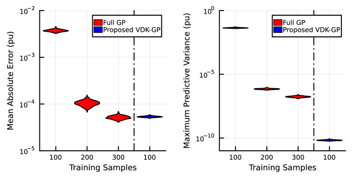
Figure 6: Comparing full GP and proposed VDK-GP for learning $V_{1}$ within $\pm 10\%$ hypercube for 500-Bus system i.e. 1000-dimensional injection space. All results are of 500 random trials with 1000 out-of-sample testing samples. Both figures have y-axis in log-scale.

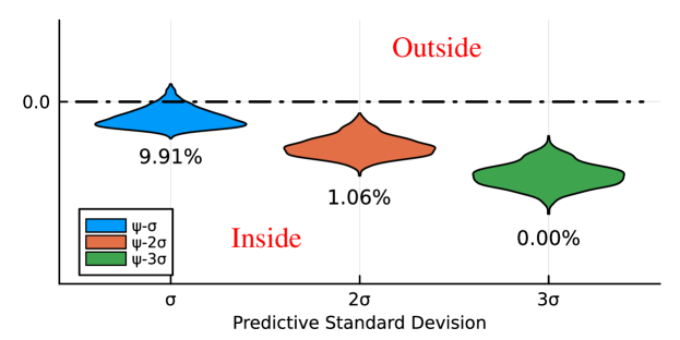
Figure 7: Percentage of absolute error $\psi(\mathbf{s})=\big{|}\mu_{f}(\mathbf{s})-V_{22}(\mathbf{s})\big{|}$ values outside different confidence regions constructed using predictive standard deviation $\sigma$ for VDK-GP learning of $V_{22}$ in 118-Bus system. We use 100 training samples and 3000 testing samples.

A key advantage of GP over other learning methods like DNNs is its ability to provide confidence intervals without additional computations, in the form of predictive variance. Hence, it is important to analyze how many samples fall within different confidence regions? Fig. 7 shows difference between error and various confidence levels ($\sigma,2\sigma,3\sigma$). The portion of violins above zero will indicate samples for which error is larger than confidence level. As depicted in Fig. 7, the percentage of samples outside the confidence interval rapidly decreases with $3\sigma$. This result shows that, similar to standard GP power flow [17], confidence intervals obtained using the proposed VDK-GP can provide a meaningful measure of model performance. In addition to evaluating the performance using metrics like MAE, ME, and MPV, it is crucial to assess the extrapolation behavior of the proposed method. Fig. 8 illustrates the performance of VDK-GP based ACPF model when trained within $\pm 10\%$ hypercube and tested on larger hypercubes up to $\pm 25\%$. Evidently, the error steadily increases when the testing set is sampled from beyond the training hypercube. However, even under extreme testing conditions ($\pm 25\%$), MAE remains on the order of $10^{-4}$, which is one order of magnitude higher than the error within training hypercube. By utilizing update methods of GP [10], it is straightforward to include additional samples from larger hypercubes to enhance the performance of the existing model.

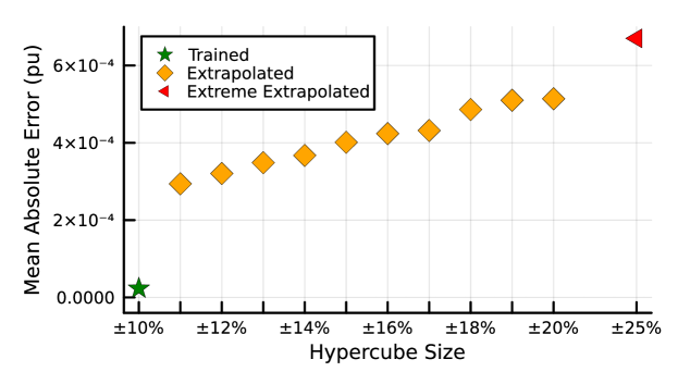
Figure 8: Extrapolation of VDK-GP model trained within $\pm 10\%$ hypercube for 118-Bus system (256 random variables). Learning conditions are same as shown in Fig. 4. All are MAE results are obtained in out-of-sample fashion using 1000 random samples within the given hypercube.

To compare the proposed method’s performance, we use a DNN with three layers and 1000 neurons in each layer [7]. We use Flux.jl with standard settings of ADAM solver to optimize hyper-parameters. Batch size is 5 and Epochs are set as 200. Table II, shows the MAE performance of the DNN along with corresponding VDK-GP performance for 118-Bus system. It is clear that the proposed VDK-GP outperforms the standard DNN model by one order of magnitude in MAE performance. Moreover, the DNN does not provide any predictive uncertainty information and thus not directly suitable as a surrogate for Bayesian optimization (BO) [23].

TABLE II: Performance of DNN and Proposed VDK-GP using 100 Training Samples in 118-Bus System

Node	MAE (pu)
	Proposed	DNN
1	$5.22\times 10^{-5}$	$1.89\times 10^{-4}$
43	$8.70\times 10^{-5}$	$9.77\times 10^{-4}$
117	$2.26\times 10^{-5}$	$9.05\times 10^{-4}$

IV-B Active Learning Performance

For performance validation of the proposed network-swipe AL method, we start with one random sample and perform three network-swipes (step 3 of Algorithm 1 repeated three times sequentially) to obtain the next training sample. Fig. 9 shows performance of network-swipe AL when applied to learn $V_{1}$ for the 118-Bus system (same as in Fig. 4). The proposed AL method outperforms the best model obtained in 500 random trials of the proposed VDK-GP by obtaining a lower MAE, as depicted in Fig. 9(a). Numerical performance comparison in Table III shows more than 1.5 fold improvement for both error indicators (MAE and ME) by a random AL trial (Fig. 9) with respect to mean performance of 500 random trials of Full GP and VDK-GP (Fig. 4) .

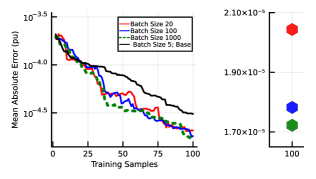
(a) MAE (pu) over 1000 testing samples.

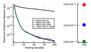
(b) MPV (pu) over 1000 testing samples.

Figure 9: Network-swipe AL’s performance for learning $V_{1}$ in $\pm 10\%$ hypercube for 118-Bus system. Base is without hyper-parameter tuning during AL and shows the impact of hyper-parameter tuning on performance. Right sub-figures show 100-th sample results. Left sub-figures have y-axis in log-scale.

TABLE III: Error performance and sample complexity comparison for $V_{1}$ learning 118-Bus system

	Learning Method (Training Samples)
	Full GP (100)	VDK-GP (100)	AL (100)
MAE $\times 10^{-5}$	3.98	2.66	1.72
ME $\times 10^{-5}$	17.1	11.5	6.98
#PF	5$\times 10^{4}$	5$\times 10^{4}$	100
– Full GP & VDK-GP: Mean over 500 random trails
– AL: Random trial with batch size 100
– #PF: Total number of ACPF solutions required

The network-swipe AL is designed to work with the proposed graph-structured VDK. Thus, the reason of the performance gain is the inherent structure present in VDK-GP, which is absent in the full GP. Fig. 10 illustrates this reasoning by comparing the performance of network-swipe AL for both Full GP and proposed VDK-GP on the 500-Bus system. Note that the batch size for Full GP’s AL trial is 10 times more than that for proposed VDK-GP. It is clear that there is an order of magnitude difference in performance. Among the 500 random trials in Fig. 10, the best-performing instance of full GP has a per unit MAE value of $4.05\times 10^{-5}$, and the proposed VDK-GP’s best result is $4.96\times 10^{-5}$. Both of these best instances are outperformed by the network-swipe AL with VDK, which achieves an MAE of $2.68\times 10^{-5}$ in the trial shown in Fig. 10. Table IV compares the errors and shows more than two fold improvement by using the proposed network-swipe AL over VDK-GP with same training dataset.

From Fig. 9 and Fig. 10, it can be observed that the MAE-Training Sample curves do not exhibit the same smoothness in their decrease as the MPV-Training Sample curves. This disparity can be attributed to the ’information gain’ measure, which is closely related to enhancing the comprehension of the function over the input space, consequently reducing prediction uncertainty. However, it is important to note that predictive variance is not a direct proxy for generalization error. Any proxy for generalization error would require labeled data, increasing the sample complexity. Furthermore, the key advantage of AL lies in its reliance solely on input vectors (injections), as evident from Eq. (6). This characteristic sets AL apart from random trials, which require a large number of power flow solutions. By achieving lower predictive uncertainty through AL, we can subsequently obtain lower generalization error, as reflected in the MAE results. The strong positive correlation observed between MPV and MAE demonstrates the ability of the proposed AL method to effectively exploit this relationship.

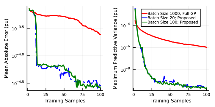
Figure 10: Network-swipe AL’s performance for full GP and proposed VDK-GP for learning $V_{1}$ within $\pm 10\%$ hypercube for 500-Bus system. Left sub-figure shows superior performance in terms of MAE (pu) while right sub-figure shows MPV (pu) performance over 1000 out-of-sample testing samples. Both figures have y-axis in log-scale.

TABLE IV: Error performance and sample complexity comparison for $V_{1}$ learning 500-Bus system

	Learning Method (Training Samples)
	Full GP (300)	VDK-GP (100)	AL (100)
MAE $\times 10^{-5}$	5.22	5.35	2.68
ME $\times 10^{-5}$	22.4	23.3	11.0
#PF	15$\times 10^{4}$	5$\times 10^{4}$	100
– Full GP & VDK-GP: Mean over 500 random trails
– AL: Random trial with batch size 100
– #PF: Total number of ACPF solutions required

Results for Large Test-case: We also test our proposed method over a large 1354-Bus test system with the $\pm 10\%$ hypercube, considering all load buses with uncertain real and reactive power injections. While limiting ourselves to power flow feasibility, we tested on $V_{5}$, which has a total variation of 0.0128 (pu) (maximum - minimum) and remains within acceptable voltage limits (0.9-1.1 pu). Fig. 11 shows the comparative performance of the proposed VDK-GP and Full GP. The green and black horizontal lines indicate the best-performing models out of 25 random trial models of the proposed VDK-GP (100 training samples) and Full GP (200 training samples), respectively, in Fig. 11. The MAE is 0.000907 (pu) and ME is 0.00352 (pu) with 100 training samples, using the proposed network-swipe AL (blue curves in Fig. 11). It is clear that the a single run of the proposed network-swipe AL outperforms best performance of 25 random trials of both proposed and Full GP. Table V shows the number of power flow samples required to obtain results in Fig. 11, clearly indicating advantage of using AL.

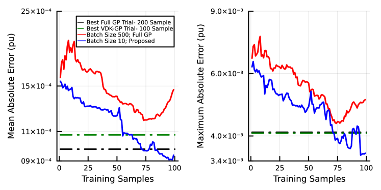
Figure 11: Network-swipe AL’s performance for full GP and proposed VDK-GP for learning $V_{5}$ within $\pm 10\%$ hypercube for 1354-Bus system. Green (black) horizontal lines indicate best performance of Full GP (proposed VDK-GP) among 25 random trials using 200 (100) training samples. Left sub-figure shows superior performance in terms of MAE (pu) while right sub-figure shows ME (pu) performance over 1000 out-of-sample testing samples. Both figures have y-axis in log-scale. Note that AL with Full GP (red line) has Batch size of 500 instead of proposed method’s (blue line) 10 only.

TABLE V: Sample complexity comparison for $V_{5}$ learning in 1354-Bus system

	Learning Method (Training Samples)
	Full GP (200)	VDK-GP (100)	AL (100)
#PF	5000	2500	100
– #PF: Total number of ACPF solutions required

IV-C Effect of Depth

The proposed VDK-GP allows to explore the effect of distance of injections on a particular node voltage. An intuitive way to do so is to analyze effect of inclusion of NNKs at different depths on learning quality. ”Fig. 12 shows the relationship between learning error and the number of kernels included in VDK (5) as a function of depth or layers. Here, the notion of depth or layers is same as described in Fig. 3. It is clear that the error-depth relationship is not linear and has abrupt decays. Interestingly, the learning quality deteriorates with more kernel inclusions up to a certain depth, under fixed hyper-parameter learning conditions (constant initial hyper-parameters, learning rate, and number of iterations). Although the change in MAE is smaller compared to improvements at higher depths, this indicates that each depth (and therefore each NNK) does not have the same dependency on target voltage. Furthermore, all three voltage functions reach very close to the full VDK values at the 10th layer mark. From the right sub-figure, layers 1 to 10 contain 264, 314, and 240 NNKs for the 30th, 33rd, and 34th voltage learning, respectively. This indicates that approximately 40% of the network has a minimal effect on the target voltages. Note that this dependency analysis also considers the effects of different injections values at these nodes. Based on acceptable error levels for the desired application (which can be as low as that achieved by the first layer inclusion only), different depth levels can be adopted for voltage function learning. This depth effect also opens up the possibility of using the proposed VDK-GP for network-partitioning type problems, which will be explored in future research.

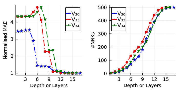
Figure 12: Effect of depth on learning quality of three different voltage function in 500-Bus system (left sub-figure) along with number of NNKs included at different depths or layers for different nodes (right sub-figure). The results consider full VDK representation at maximum depth.

IV-D Applications: Uncertainty Quantification

The purpose of UQ is to identify the probability distribution of the state variables, such as node voltage, given an input injection distribution. However, analytical models fail when the injection distribution faced by the model is different from what they were trained on[17]. In contrast, the proposed VDK-GP model shows robustness against distributional shifts, where testing injection distribution in different than training ones, and provides subspace-wise approximation. This is due to the fact that GP are generative models and work on point-by-point evaluation after training. Therefore, the underlying distribution of the input injection does not significantly affect the prediction performance, as long as the point lies near the training set, i.e., within the training hypercube. Fig. 13 shows distributions obtained for three different node voltages by training sampled taken from $\pm 10\%$ hypercube uniformly. Although VDK-GP model is trained using uniform samples, it is able to provide accurate voltage distributions for both normal and beta injection distributions. Furthermore, for node 43, the KL-divergence between the combined test and true distributions in Fig. 13 is $1.36\times 10^{-9}$. This indicates that proposed VDK-GP models are distributionally robust (non-parametric and subspace-wise approximations [17]). Future work will involve building voltage envelope identification by using the proposed VDK-GP as a surrogate model in BO [23].

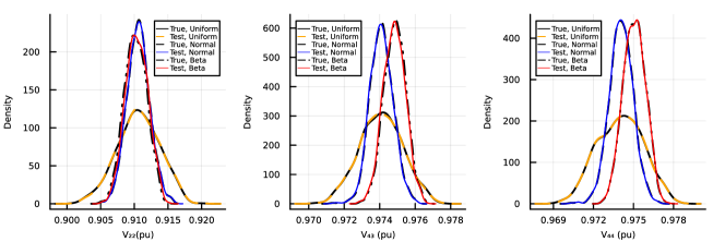
Figure 13: Density functions for uncertainty quantification in 118-Bus system for three different node voltages. Training is done using 100, 110 and 120 samples for $V_{22}$, $V_{43}$ and $V_{44}$ respectively, taken from uniform samples. 1000 testing samples are used to plot all density curves.

V Conclusion

In conclusion, this paper introduces a novel graph-structured kernel, the vertex degree kernel (VDK), designed to enhance power flow learning using Gaussian Process (GP) with an additive structure inspired by physics. VDK effectively leverages network graph information, providing a promising approach for improved voltage-injection relationship modeling. The results obtained demonstrate the superiority of VDK-GP over the full GP, showcasing a substantial reduction in sample complexity. Moreover, VDK-GP yields higher confidence models for medium to large-scale power systems. The network-swipe algorithm further enhances model performance by employing intelligent data selection, maximizing information gain without reliance on labeled data. Importantly, the proposed method exhibits superiority over standard learning approaches in uncertainty quantification applications, making it a valuable addition to real-world power system scenarios. For future directions, the additive structure and active learning capabilities of VDK-GP pave the way for developing Bayesian optimization-based methods tailored for large-scale power systems. These advancements have the potential to solve power system planing and operational problems like chance-constrained optimal power flow, hosting capacity, distributed or control source sizing and operating envelop identification etc., offering more efficient and accurate solutions amidst complex and uncertain conditions. In summary, the introduction of VDK-GP and the network-swipe algorithm contributes significant insights to power flow modeling and optimization for large-scale power systems. By harnessing graph-structured kernels and active learning techniques, this research lays the foundation for further advancements in Bayesian approaches for power system optimization.

References

- [1] D. K. Molzahn, I. A. Hiskens et al., “A survey of relaxations and approximations of the power flow equations,” Foundations and Trends® in Electric Energy Systems, vol. 4, no. 1-2, pp. 1–221, 2019.
- [2] M. Jia et al., “Tutorial on data-driven power flow linearization-part i: Challenges and training algorithms,” Submitted, 2023.
- [3] S. Misra, D. K. Molzahn, and K. Dvijotham, “Optimal adaptive linearizations of the ac power flow equations,” in 2018 Power Systems Computation Conference (PSCC). IEEE, 2018, pp. 1–7.
- [4] D. Deka, S. Backhaus, and M. Chertkov, “Structure learning in power distribution networks,” IEEE Transactions on Control of Network Systems, vol. 5, no. 3, pp. 1061–1074, 2017.
- [5] L. Guo et al., “Data-driven power flow calculation method: A lifting dimension linear regression approach,” IEEE Trans. on Power Systems, vol. 37, no. 3, pp. 1798–1808, 2022.
- [6] G. E. Karniadakis et al., “Physics-informed machine learning,” Nature Reviews Physics, vol. 3, no. 6, pp. 422–440, 2021.
- [7] M. Gao, J. Yu, Z. Yang, and J. Zhao, “A physics-guided graph convolution neural network for optimal power flow,” IEEE Transactions on Power Systems, 2023.
- [8] X. Hu, H. Hu, S. Verma, and Z.-L. Zhang, “Physics-guided deep neural networks for power flow analysis,” IEEE Trans. on Power Systems, vol. 36, no. 3, pp. 2082–2092, 2020.
- [9] K. Chen and Y. Zhang, “Physics-guided residual learning for probabilistic power flow analysis,” arXiv preprint arXiv:2301.12062, 2023.
- [10] C. K. Williams and C. E. Rasmussen, Gaussian processes for machine learning. MIT press Cambridge, MA, 2006, vol. 2, no. 3.
- [11] P. Pareek and H. D. Nguyen, “Gaussian process learning-based probabilistic optimal power flow,” IEEE Trans. on Power Systems, vol. 36, no. 1, pp. 541–544, 2020.
- [12] M. Mitrovic et al., “Data-driven stochastic ac-opf using gaussian process regression,” International Journal of Electrical Power & Energy Systems, vol. 152, p. 109249, 2023.
- [13] M. Jalali et al., “Inferring power system dynamics from synchrophasor data using gaussian processes,” IEEE Trans. on Power Systems, vol. 37, no. 6, pp. 4409–4423, 2022.
- [14] M. K. Singh et al., “Physics-informed transfer learning for voltage stability margin prediction,” in 2023 IEEE International Conference on Acoustics, Speech and Signal Processing (ICASSP), 2023, pp. 1–5.
- [15] Y. Xu et al., “Probabilistic power flow based on a gaussian process emulator,” IEEE Trans. on Power Systems, vol. 35, no. 4, pp. 3278–3281, 2020.
- [16] ——, “A data-driven nonparametric approach for probabilistic load-margin assessment considering wind power penetration,” IEEE Trans. on Power Systems, vol. 35, no. 6, pp. 4756–4768, 2020.
- [17] P. Pareek and H. D. Nguyen, “A framework for analytical power flow solution using gaussian process learning,” IEEE Trans. on Sustainable Energy, vol. 13, no. 1, pp. 452–463, 2021.
- [18] D. K. Duvenaud et al., “Additive gaussian processes,” Advances in neural information processing systems, vol. 24, 2011.
- [19] X. Lu et al., “Additive gaussian processes revisited,” in International Conference on Machine Learning. PMLR, 2022, pp. 14 358–14 383.
- [20] J. Liu and P. Srikantha, “Kernel structure design for data-driven probabilistic load flow studies,” IEEE Trans. on Smart Grid, vol. 13, no. 4, pp. 2679–2689, 2022.
- [21] B. Settles, “Active learning literature survey,” 2009.
- [22] C. Riis et al., “Bayesian active learning with fully bayesian gaussian processes,” Advances in Neural Information Processing Systems, vol. 35, pp. 12 141–12 153, 2022.
- [23] P. I. Frazier, “A tutorial on bayesian optimization,” arXiv preprint arXiv:1807.02811, 2018.
- [24] N. Srinivas et al., “Information-theoretic regret bounds for gaussian process optimization in the bandit setting,” IEEE Trans. on Information Theory, vol. 58, no. 5, pp. 3250–3265, 2012.
- [25] B. Huang and J. Wang, “Applications of physics-informed neural networks in power systems-a review,” IEEE Transactions on Power Systems, vol. 38, no. 1, pp. 572–588, 2022.
- [26] P. Rolland et al., “High-dimensional bayesian optimization via additive models with overlapping groups,” in International conference on artificial intelligence and statistics. PMLR, 2018, pp. 298–307.
- [27] C. Li et al., “High dimensional bayesian optimization using dropout,” in Proceedings of the 26th International Joint Conference on Artificial Intelligence, 2017, pp. 2096–2102.
- [28] J. J. Grainger and W. D. Stevenson, Power System Analysis, 2003.
- [29] A. Krause and C. E. Guestrin, “Near-optimal nonmyopic value of information in graphical models,” arXiv preprint arXiv:1207.1394, 2012.
- [30] K. Kandasamy, J. Schneider, and B. Póczos, “High dimensional bayesian optimisation and bandits via additive models,” in International conference on machine learning. PMLR, 2015, pp. 295–304.
- [31] Y. You et al., “Large batch optimization for deep learning: Training bert in 76 minutes,” arXiv preprint arXiv:1904.00962, 2019.
- [32] J. González, Z. Dai, P. Hennig, and N. Lawrence, “Batch bayesian optimization via local penalization,” in Artificial intelligence and statistics. PMLR, 2016, pp. 648–657.
- [33] S. Babaeinejadsarookolaee et al., “The power grid library for benchmarking ac optimal power flow algorithms,” arXiv preprint arXiv:1908.02788, 2019.
- [34] S. Lotfi et al., “Bayesian model selection, the marginal likelihood, and generalization,” in International Conference on Machine Learning. PMLR, 2022, pp. 14 223–14 247.