Cosmic inflation and $(g-2)_{\mu}$ in minimal gauged $L_{\mu}-L_{\tau}$ model

Abstract

The minimal $U(1)_{L_{\mu}-L_{\tau}}$ gauge symmetry extended Standard Model (SM) is a well motivated framework that resolves the discrepancy between the theoretical prediction and experimental observation of muon anomalous magnetic moment. We envisage the possibility of identifying the beyond Standard Model Higgs of $U(1)_{L_{\mu}-L_{\tau}}$ sector, non-minimally coupled to gravity, as the inflaton in the early universe, while being consistent with the $(g-2)_{\mu}$ data. Although the structure seems to be trivial, we observe that taking into consideration of a complete cosmological history starting from inflation through the reheating phase to late-time epoch along with existing constraints on $U(1)_{L_{\mu}-L_{\tau}}$ model parameters leave us a small window of allowed reheating temperature. This further results into restriction of $(n_{s}-r)$ plane which is far severe than the one in a generic non-minimal quartic inflationary set up.

I Introduction

The observed discrepancy between the measured and the theoretically predicted value of muon anomalous magnetic moment $(g-2)_{\mu}$ prompts us to look for beyond Standard Model (SM) physics. Such disagreement was previously reported by Brookhaven National Laboratory (BNL) E821 experiment Bennett et al. (2006) and also recently measured by Fermilab E989 experiment Abi et al. (2021); MUON G-2 collaboration . A precise analysis of the combined experimental data reveals Abi et al. (2021),

$$\Delta a_{\mu}=a_{\mu}^{\rm exp}-a_{\mu}^{\rm SM}=(249\pm 48)\times 10^{-11},$$ (1)

where we define $a_{\mu}=\left(\frac{g-2}{2}\right)_{\mu}$. The observed value of $a_{\mu}$ deviates from the SM predicted value Aoyama et al. (2020) at $4.2\sigma$ confidence level .

The minimal gauged $U(1)_{L_{\mu}-L_{\tau}}$ model, being anomaly free He et al. (1991a, b) provides excellent scope to address the observed excess of the $(g-2)_{\mu}$ Baek et al. (2001); Ma et al. (2002); Baek (2016); Heeck and Rodejohann (2011); Banerjee et al. (2021). In the minimal version of $U(1)_{L_{\mu}-L_{\tau}}$ gauge theory, only second and third generations of SM leptons are charged under $U(1)_{L_{\mu}-L_{\tau}}$ symmetry and one also has a SM gauge singlet scalar. The gauge singlet scalar receives a non-zero vacuum expectation value (vev) which spontaneously breaks the $U(1)_{L_{\mu}-L_{\tau}}$ symmetry. It is also possible to extend the minimal gauged $U(1)_{L_{\mu}-L_{\tau}}$ model by three right handed (RH) neutrinos without introducing any gauge anomaly, in order to accommodate correct order of neutrino mass and mixings, satisfying the neutrino oscillation data via standard seesaw mechanism Asai et al. (2017). In this work, we adhere to the minimal gauged $U(1)_{L_{\mu}-L_{\tau}}$ model.

In another front, the cosmic microwave background (CMB) data reveals that our Universe is spatially flat, homogeneous, and isotropic which remain unexplained in the standard description of big bang cosmological theory. To interpret these shortcomings of the big bang cosmology, theory of cosmic inflation is postulated Guth (1987); Linde (1987); Starobinsky (1980); Albrecht and Steinhardt (1982). During inflation, the Hubble parameter of the Universe remains almost constant, driving the Universe to undergo a phase of exponential expansion. Cosmic inflation also generates nearly scale invariant primordial scalar and tensor perturbations at super-horizon scale which seed formation of large scale structures while re-entering the horizon at a later stage.

Linking an inflationary scenario with a well motivated particle physics framework is an interesting exercise to pursue. There exists numerous works in this direction considering various types of supersymmetric and non-supersymmetric extensions of the SM of particle physics. The simplest possibility is to identify the SM Higgs as inflaton Bezrukov (2013), the field responsible for the cosmic inflation. However, the tree level Higgs potential fails to provide a successful inflationary scenario and one requires to introduce non-minimal coupling ($\xi$) of the SM Higgs with gravity to make the SM Higgs inflation compatible with experimental data. It turns out that one needs a large $\xi\sim\mathcal{O}(10^{4})$ to be in agreement with the observed curvature perturbations Bezrukov and Shaposhnikov (2008), which gives rise to the question of naturalness from unitarity point of view Barbon and Espinosa (2009); Lerner and McDonald (2010). This issue can be possibly eliminated if the inflaton is identified with a gauge singlet scalar. Presence of gauge singlet scalar is common in different Abelian gauge extended beyond standard model (BSM) frameworks.

Figure 1: The evolution of comoving Hubble radius $\frac{1}{(aH)}$ is shown as function of a scale factor of the Universe. The red colored line indicates the evolution of comoving Hubble radius during inflation that exited the horizon at $a=a_{k}$, for a particular number of inflationary e-fold $N_{\rm e}$. The inflation ends at $a=a_{\rm end}$ and the evolution of $\frac{1}{(aH)}$ during inflaton oscillation era is indicated by solid cyan colored line. At $a=a_{\rm RH}$, the reheating of the Universe is completed and afterwards the RD universe prior to BBN sets in. The solid blue line marks the evolution of $\frac{1}{(aH)}$ for a standard observable Universe, extrapolated up to $a=a_{\rm RH}$.

In this work, we analyse the dynamics of cosmic inflation in the minimal $U(1)_{L_{\mu}-L_{\tau}}$ framework where the SM gauge singlet scalar is identified with the inflaton. We have adopted the conventional inflationary set up with non-minimal coupling of inflaton to gravity Park and Yamaguchi (2008); Okada et al. (2010); Bezrukov and Gorbunov (2013); Linde (2015) in order to satisfy the cosmological inflationary constraints as provided by Planck+BICEP/Keck Akrami et al. (2020); Ade et al. (2022). In particular we examine the viability of $(g-2)_{\mu}$ satisfying parameter space in providing a consistent cosmological scenario from the onset of primordial inflation to the end of matter-radiation equality with the intermediate reheating phase Albrecht et al. (1982); Dolgov and Kirilova (1990); Kofman et al. (1994); Shtanov et al. (1995). We observe that the measurements of $(g-2)_{\mu}$ along with other observational constraints restrict the $U(1)_{L_{\mu}-L_{\tau}}$ breaking scale to remain within $\sim(13-75)$ GeV. This estimate of $U(1)_{L_{\mu}-L_{\tau}}$ breaking scale along with the inflationary constraints determine the inflaton mass. The inflaton mass is an important quanitity which decides the dynamics of the inflaton oscillations and sets the kinematics of the energy transfer processes of inflaton to radiation. For a given particular inflation model with fixed number of inflationary e-folds the evolution of the Hubble horizon can be easily determined. On the other hand from observations, we know the dynamics of standard Hubble horizon as a function of scale factor from radiation dominated epoch till the present time. Therefore, to enter into a standard radiation dominated phase from the inflaton dominated Universe, the Hubble horizon during inflaton decay (reheating) must match the standard one before the onset of Big Bang Nucleosynthesis (BBN) Liddle and Leach (2003); Martin and Ringeval (2010); Drewes et al. (2017). We present a schematic diagram of this evolution as a function of scale factor in Fig. 1. This observation tells us the completion time (or scale factor) of inflaton decay which in turn fixes the inflaton interaction strength with the SM particles for a given number of inflationary e-fold.

In our case, the energy transfer of inflation sector to radiation bath occurs via perturbative decay of inflaton, controlled by Higgs-singlet scalar mixing $\theta$. Note that the inflaton mass - $\sin\theta$ plane is constrained by various experimental observations in the sub-GeV inflaton mass range. We study the correspondence of the inflationary parameters namely number of e-folds during inflation ($N_{\rm e}$) and non-minimal coupling of inflaton with inflaton mass and $\theta$. Such correspondence further add new constraints on the inflaton mass - $\theta$ plane, mainly arising from the stability of the inflaton potential during inflation, positivity of e-foldings in different epochs and the completion of inflaton decay before BBN. We find that these new constraints along with existing ones on the inflaton mass - $\theta$ plane significantly restrict the amount of both $N_{\rm e}$ and $\xi$ and thereby leaving strong impact on the prediction of inflationary observables such as $n_{s}$ and $r$. In the present study, considering the minimal version of $L_{\mu}-L_{\tau}$ model, we have obtained the predictions for $n_{s}$ and $r$ in the parameter region which is in agreement with $(g-2)_{\mu}$ data. Our results for ($n_{s},r$) turn out to be very predictive and much more restrictive than the one in a generic non-minimal quartic inflationary set up.

The plan of the paper is as follows. In section II we discuss the $U(1)_{L_{\mu}-L_{\tau}}$ model briefly. In the next section, section III we explain the methodology adopted in this work. Section IV describes the dynamics of the inflaton after inflation till reheating. In section V and VI we discuss the results and conclusions respectively.

II $L_{\mu}-L_{\tau}$ Model

In the minimal $U(1)_{L_{\mu}-L_{\tau}}$ gauged model, the gauge anomalies get cancelled between $\mu$ and $\tau$ leptonic generations, even without the introduction of any additional chiral fermions. One also incorporates a SM gauge singlet scalar field ($\varphi$) that receives non-zero VEV and breaks the $U(1)_{L_{\mu}-L_{\tau}}$ gauge symmetry spontaneously. The scalar sector of the $U(1)_{L_{\mu}-L_{\tau}}$ gauged framework have following structure of the potential.

$$V(|H|,|\varphi|)=\lambda_{\phi}\left(|\varphi|^{2}-\frac{v^{\prime 2}}{2}\right)^{2}+\lambda_{H}\left(|H|^{2}-\frac{v^{2}_{H}}{2}\right)^{2}+\lambda_{H\phi}\left(|H|^{2}-\frac{v^{2}_{H}}{2}\right)\left(|\varphi|^{2}-\frac{v^{\prime 2}}{2}\right),$$ (2)

where we have assumed all dimensionful and dimensionless couplings as real and positive. We have assigned ‘+2’ $U(1)_{L_{\mu}-L_{\tau}}$ charge to the $\varphi$ field. After the electroweak symmetry breaking (EWSB), considering unitary gauge, we write,

$$H=\begin{pmatrix}0\\ \frac{v_{H}+h}{\sqrt{2}}\end{pmatrix}\textrm{~{}~{}~{}~{}and~{}~{}~{}~{}}\varphi=\frac{1}{\sqrt{2}}(v^{\prime}+\phi+iA).$$ (3)

The scalar mass squared matrix contains off-diagonal terms and after EWSB, mixing between $h$ and $\phi$ takes place. The mass eigenstates ($\phi_{1}$ and $\phi_{2}$) are related to $h$ and $\phi$ as,

$$\begin{bmatrix}h\\ \phi\end{bmatrix}=\begin{bmatrix}\cos\theta&-\sin\theta\\ \sin\theta&\cos\theta\end{bmatrix}\begin{bmatrix}\phi_{1}\\ \phi_{2}\end{bmatrix},$$

where $\theta$ is the mixing angle between $h$ and $\phi$. The mixing angle $\theta$ and the masses $m_{\phi_{1}}$ and $m_{\phi_{2}}$ of the mass eigenstates $\phi_{1}$ and $\phi_{2}$ are then given by,

$$\tan 2\theta = \frac{2v^{\prime}v_{H}\lambda_{H\phi}}{m_{h}^{2}-m_{\phi}^{2}}$$ (4)

$$m_{\phi_{1}}^{2} = m_{h}^{2}-\left(m_{\phi}^{2}-m_{h}^{2}\right)\frac{\sin^{2}\theta}{1-2\sin^{2}\theta}$$ (5)

$$m_{\phi_{2}}^{2} = m_{\phi}^{2}+\left(m_{\phi}^{2}-m_{h}^{2}\right)\frac{\sin^{2}\theta}{1-2\sin^{2}\theta},$$ (6)

where $m_{\phi}=\sqrt{2\lambda_{\phi}}v^{\prime}$, $m_{h}=\sqrt{2\lambda_{H}}v_{H}=125$ GeV. For small $\theta$, which is the scenario we are interested in, $\phi_{1}$ and $\phi_{2}$ are mostly the SM Higgs $h$ and inflaton $\phi$ respectively. The mass of the mostly inflaton state $\phi_{2}$ is then $m_{\phi_{2}}\sim m_{\phi}$, whereas $m_{\phi_{1}}\sim m_{h}$.

In the broken phase of $SU(2)_{L}\times U(1)_{Y}\times U(1)_{L_{\mu}-L_{\tau}}$, we also write the following Lagrangian,

$$\mathcal{L}=\mathcal{L}_{\rm SM}-\frac{1}{4}Z^{\prime\alpha\beta}Z^{\prime}_{\,\alpha\beta}+\frac{m_{Z^{\prime}}^{2}}{2}Z^{\prime\alpha}Z^{\prime}_{\alpha}+Z^{\prime}_{\alpha}J_{\mu\tau}^{\alpha},$$ (7)

where $Z^{\prime}_{\alpha\beta}=\partial_{\alpha}Z^{\prime}_{\beta}-\partial_{\beta}Z^{\prime}_{\alpha}$ is the field strength tensor for the $U(1)_{L_{\mu}-L\tau}$ gauge symmetry, $m_{Z^{\prime}}=2g^{\prime}v^{\prime}$ represents the mass of the new gauge boson $Z^{\prime}$. The $J_{\mu\tau}^{\alpha}$ stands for the $\mu-\tau$ current as expressed as,

$$J_{\mu\tau}^{\alpha}=g^{\prime}(\overline{\mu}\gamma^{\alpha}\mu+\overline{\nu_{\mu}}\gamma^{\alpha}P_{L}\nu_{\mu}-\overline{\tau}\gamma^{\alpha}\tau-\overline{\nu_{\tau}}\gamma^{\alpha}P_{L}\tau_{\mu}),$$ (8)

where $P_{L}=\frac{1}{2}(1-\gamma_{5})$ is the left chiral operator and $g^{\prime}$ stands for the $U(1)_{L_{\mu}-L_{\tau}}$ gauge coupling. Although the tree level kinetic mixing is assumed to be zero, at loop level, $Z^{\prime}$ mixes with the photon that leads to coupling of $Z^{\prime}$ with electrons Kamada and Yu (2015); Araki et al. (2017).

The ability of minimal $U(1)_{L_{\mu}-L_{\tau}}$ framework to accommodate the experimentally observed value of $(g-2)_{\mu}$ has long been recognized. This contribution to the anomalous magnetic moment of the muon ($\Delta a_{\mu}$) arises dominantly from the loop involving the $Z^{\prime}$ boson, which can be expressed as follows Baek et al. (2001); Ma et al. (2002):

$$\Delta a_{\mu}=\frac{{g^{\prime}}^{2}}{4\pi^{2}}\int_{0}^{1}dx\,\frac{x(1-x)^{2}}{(1-x)^{2}+rx},$$ (9)

where $r=\left(\frac{M_{Z^{\prime}}}{m_{\mu}}\right)^{2}$, with $m_{\mu}$ being the $\mu$ mass.

Figure 2: Existing constraints on the $m_{Z^{\prime}}-g^{\prime}$ plane is shown. The region in blue color successfully accommodates the $(g-2)_{\mu}$ data. Constraints from BABAR Lees et al. (2016), Borexino Bellini et al. (2014) and CCFR Mishra et al. (1991) are highlighted with green, brown and purple colors respectively. The two dashed lines correspond to $v^{\prime}=13$ GeV and $v^{\prime}=75$ GeV respectively. The upcoming sensitivities of NA62 and Belle II are taken from Krnjaic et al. (2020) and Aggarwal et al. (2022) respectively.

In Fig. 2, the region, highlighted in blue represents the parameter space where the experimentally preferred values can be accommodated successfully. The stringent constraints on $m_{Z^{\prime}}-g^{\prime}$ plane appear due to neutrino interaction of $Z^{\prime}$ at CCFR Mishra et al. (1991) and solar neutrino scattering at Borexino Bellini et al. (2014). Additionally four $\mu$-final state searches at BABAR Lees et al. (2016) strongly restrict the $m_{Z^{\prime}}-g^{\prime}$ plane. Future observations from NA62 Krnjaic et al. (2020) and Belle II (50 ab^-1) Aggarwal et al. (2022) can potentially rule out the whole $(g-2)_{\mu}$ satisfying parameter space. Taking into account all the relevant existing constraints we infer that present experimentally preferred value of $\Delta a_{\mu}$ requires $13\,{\rm GeV}\lesssim v^{\prime}\lesssim 75\,{\rm GeV}$ as depicted by two black dotted line in Fig. 2.

III The proposed methodology

At the onset of inflation, we consider the field $\phi$ as the sole species to remain abundant in the early Universe. The action in that case is given by,

$$S=\int{\rm d}^{4}x\sqrt{-g}\left[-\frac{M_{P}^{2}}{2}\left(1+\frac{\xi\phi^{2}}{M_{P}^{2}}\right)R+{1\over 2}g^{\mu\nu}\partial_{\mu}\phi\,\partial_{\nu}\phi-V(\phi)\right].$$ (10)

Here $V(\phi)$ is the inflationary potential, expressed as

$$V\supset\frac{\lambda_{\phi}}{4}\phi^{4}+\frac{1}{2}\xi\phi^{2}R,$$ (11)

with the role of the inflaton being served by the CP even neutral scalar $\phi$. Here $R$ is the Ricci scalar and $\xi$ stands for the non-minimal coupling of $\phi$ to gravity. Note that the non-minimal interaction of $\phi$ with gravity originally arises from $\xi|\varphi|^{2}R$ term and hence does not violate the $U(1)_{L_{\mu}-L_{\tau}}$ symmetry. Since the gravity is non-minimal here, a conformal transformation of metric is essential in order to preserve the validity of Einstein Hilbert gravity. The metric transformation is given by,

$$\bar{g}_{\mu\nu}=\Omega^{2}g_{\mu\nu},~{}\text{~{}with~{}}~{}\Omega^{2}=1+\frac{\xi\phi^{2}}{M_{P}^{2}}$$ (12)

To get rid of the non-canonical kinetic term, induced by the metric transformation, following transformation of $\phi$ is also required,

$$\frac{{\rm d}\chi}{{\rm d}\phi}=\frac{1}{\Omega^{2}}\sqrt{\Omega^{2}+6\xi^{2}\frac{\phi^{2}}{M_{P}^{2}}}$$ (13)

With these, we finally obtain the inflationary potential in the Einstein frame as defined by,

$$V_{E}(\chi)=\frac{1}{\Omega^{4}(\phi(\chi))}V_{J}(\phi(\chi))$$ (14)

where $V_{J}(\phi)=\frac{\lambda_{\phi}}{4}\phi^{4}$. It should be noted that the current setup under consideration leads to a high-scale inflationary scenario with $\chi>M_{P}$ (implying $\phi>M_{P}$ as well) during inflation. This means that the inflation has occurred at energy scales significantly higher than the EWSB scale and hence it is safe to ignore the $-\frac{1}{2}\lambda_{\phi}v^{\prime 2}|\phi|^{2}$ term from Eq.(2) during inflation. The inflaton mass at its minimum is given by $m_{\phi}\simeq m_{\phi_{2}}$ in the small $\sin\theta$ limit. A generic quartic inflationary potential Linde (1983) i.e. when $\xi=0$, is disfavored by the Planck-2018 constraints Akrami et al. (2020) due to the prediction of large tensor to scalar ratio $r\sim 0.133$ Linde (1983). The nonminimal coupling of inflaton to gravity assists into flattening of inflationary potential that further leads to the revival of a quartic inflationary set up. In this modified set up of quartic inflation, one can simply estimate the values of spectral index ($n_{s}$), $r$ and scalar curvature perturbation spectrum $P_{s}$, under the slow roll approximation and using the conventional approach Okada et al. (2010). The observed value of $P_{s}$ is $2.2\times 10^{-9}$ Akrami et al. (2020), which uniquely constrains the parameter $\lambda_{\phi}$ as a function of $\xi$. The predictions of $n_{s}$ and $r$ have no dependence on $\lambda_{\phi}$.

It is worth mentioning that inflection point inflation scenarios in a few Abelian gauge (e.g. $U(1)_{B-L}$ Okada and Raut (2017)) extended models have been widely studied, which does not require the non-minimal coupling to gravity in order to flatten the quartic inflationary potential. In these scenarios, interplay of the quantum corrections from the BSM gauge coupling and the Yukawa couplings give rise to the required flatness. However, the current model being a minimal one, does not have any additional Yukawa couplings.

Figure 3: A schematic representation of the strategy to connect $(g-2)_{\mu}$ data with the cosmological predictions for $(n_{s},r)$.

Next we describe our adopted methodology (as summarised in Fig. 3) that reveals how the satisfaction of $(g-2)_{\mu}$ data impact the predictions of the inflationary observables $(n_{s},r)$. As earlier mentioned, a consistent $\Delta a_{\mu}$ data requires $13\,{\rm GeV}\lesssim v^{\prime}\lesssim 75\,{\rm GeV}$. On the other hand, the successful dynamics of inflation in generating the observed value of scalar curvature spectrum Akrami et al. (2020) uniquely fixes $\lambda_{\phi}$ as a function of the non-minimal coupling parameter $\xi$. Choosing a particular $v^{\prime}$ within its preferred range along with $\lambda_{\phi}(\xi)$ provide us the dependence of the inflaton mass ($m_{\phi})$ on $\xi$. Now we consider the inflaton to decay into radiation perturbatively via Higgs portal  . In that case the reheating temperature of the Universe ($T_{\rm RH}$) turns out to be a function of $m_{\phi}$ and $\lambda_{H\phi}$. Now for a given number of inflationary e-fold ($N_{\rm e}$), the $T_{\rm RH}$ of the Universe cannot be arbitrary. This means for a fixed $\xi$ (or $m_{\phi}$), the $\lambda_{H\phi}$ has be to uniquely fixed as well. It is known that the $m_{\phi}-\lambda_{H\phi}$ plane is severely constrained by different existing experiments namely CHARM Bergsma et al. (1985), SN1987a Dev et al. (2020a); Krnjaic (2016), BBN etc. On the top of that, there are additional constraints arising to ensure the stability of inflaton potential during inflation and positivity of number of e-fold during inflaton oscillation and reheating. Such constraints in the $m_{\phi}-\lambda_{H\phi}$ plane strongly restricts $N_{\rm e}$ as a function of $\xi$ which in turn poses constraint in the $n_{s}-r$ plane.

IV Post-Inflationary dynamics and Reheating

After the slow-roll conditions get violated, the inflation ends and the inflaton begins to oscillate around its minimum. Initially the amplitude of the oscillation is large and the potential remains almost quartic and at later stage the quadratic term of $\phi$ starts to dominate. It is well known that the average equation of state (e.o.s) parameter during the oscillation regime is $w=\frac{n-2}{n+2}$ for a $\phi^{n}$ potential. Hence at initial phases of inflaton oscillation, $w=\frac{1}{3}$ and subsequently $w=0$ in the $\phi^{2}$ dominated phase. The transition of e.o.s parameter from $\frac{1}{3}$ to $0$ can be noticed in Fig. 1 as well. Importantly, the maximum oscillation amplitude of the inflaton at the point of transition from radiation-like phase ($w=\frac{1}{3}$) to matter-like phase $w=0$ is function of the ratio $\frac{m_{\phi}}{\sqrt{\lambda_{\phi}}}$ which is nothing but $\sqrt{2}v^{\prime}$.

Now, at Hubble horizon exit for a comoving mode $k$, we can write $k=a_{k}H_{k}$ with $a_{k}$ and $H_{k}$ being the scale factor and Hubble rate during the horizon exit of mode $k$. Here we consider $k=k_{\rm pivot}^{\rm Planck}=0.05~{}\rm Mpc^{-1}$. Then it follows,

$$\ln\left(\frac{k}{a_{k}H_{k}}\right)=\ln\left(\frac{a_{\phi,\rm rad}}{a_{k}}\frac{a_{\phi,\rm matter}}{a_{\phi,\rm rad}}\frac{a_{\rm RH}}{a_{\phi,\rm matter}}\frac{a_{k,\rm late}}{a_{\rm RH}}\frac{k}{a_{k,\rm late}H_{k}}\right)=0,$$ (15)

where $a_{\phi,\rm rad}$ denote the scale factor of the Universe at the beginning of inflaton oscillation with e.o.s. $\frac{1}{3}$ and $a_{\phi,\rm matter}$ stands for the scale factor at the cross-over where inflaton becomes matter like having $\omega=0$. $a_{\rm RH}$ corresponds to the scale factor at the end of reheating and $a_{k,\rm late}\sim 4.5\times 10^{-5}$ indicates the scale factor when $k=0.05~{}\rm Mpc^{-1}$ mode re-enters the Hubble horizon. The Eq.(15) can be further translated to,

$$N_{\rm e}+{\rm ln}\left(\frac{\rho_{\phi,\rm rad}}{\rho_{\phi,\rm matter}}\right)^{\frac{1}{4}}+{\rm ln}\left(\frac{\rho_{\phi,\rm matter}}{\rho_{\phi,\rm RH}}\right)^{\frac{1}{3}}+{\rm ln}\left(\frac{\rho_{\phi,\rm RH}}{\rho_{k,\rm late}}\right)^{\frac{1}{4}}+{\rm ln}\left(\frac{k}{a_{k,\rm late}H_{k}}\right)=0,$$ (16)

where $N_{\rm e}$ represents the number of e-fold during inflation and $\rho_{\phi,\rm rad}\simeq\frac{4}{3}V(\phi_{\rm end})$ is the energy density of inflaton at the end of inflation which also implies the onset of oscillation phase. $\rho_{\phi,\rm matter}$ is the energy stored in inflaton when the crossover happens from quartic to quadratic domination in the inflationary potential. $\rho_{\phi,\rm RH}=\frac{\pi^{2}}{30}g_{*}(T_{\rm RH})T_{\rm RH}^{4}$, the energy density of the Universe after the completion of reheating phase. Finally, $\rho_{k,\rm late}=\frac{\pi^{2}}{30}g_{*}(T_{k,\rm late})T_{k,\rm late}^{4}$ where we evaluate the $T_{k,\rm late}$ using the entropy conservation principle, $a_{k,\rm late}T_{k,\rm late}\simeq a_{0}T_{0}$. With all these inputs, the Eq.(16) relates $T_{\rm RH}$ with the quantity $N_{\rm e}$, provided the non-minimal coupling $\xi$ and $v^{\prime}$ are fixed. To note, $\lambda_{\phi}$ can be determined from the consideration of observed primordial power spectrum amplitude which in turn specifies the Hubble scale of inflation during horizon exit of mode $k$ i.e. $H_{k}$.

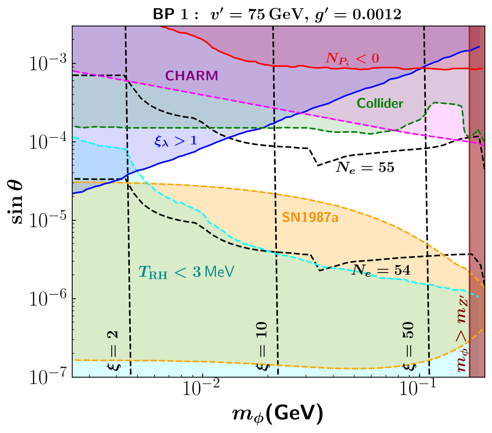
Figure 4: The correlation between inflaton sector parameters $\xi$,$N_{\rm e}$ and the scalar sector parameters is shown. Each choice of $(\xi,N_{\rm e})$ corresponds to a particular set of $(m_{\phi},\sin\theta)$. Constraints from CHARM Bergsma et al. (1985), SN1987a Dev et al. (2020a); Krnjaic (2016) and Collider Balaji et al. (2022); Dev et al. (2017); Egana-Ugrinovic et al. (2020); Dev et al. (2020b) are shown in purple, orange and green colours respectively. Other forbidden regions arising from $\xi_{\lambda}>1$, $N_{P_{i}}<0$ where $i=\{{\rm rad,\,matter}\}$ and $T_{\rm RH}<3$ MeV conditions are highlighted in blue, red and cyan respectively.

The Eq.(16) gives the value of $T_{\rm RH}$ as a function of $N_{\rm e}$ for a well defined inflationary potential. Now, in the particle physics model under discussion the inflaton decays to radiation bath via mixing with SM Higgs with inflaton decay rate $\Gamma_{\phi_{2}}=\sin^{2}\theta\times\Gamma_{h}(m_{\phi_{2}})$ (where $\Gamma_{h}(m_{\phi_{2}})$ is the SM Higgs decay rate when its mass is $m_{\phi_{2}}$), resulting the universe to enter into standard radiation domination epoch. We emphasize here once again, in this work we have restricted ourselves in such a parameter region of $\lambda_{\phi}$ such that the decay of $\phi$ into $Z^{\prime}$ is kinematically blocked, i.e. $m_{\phi}<m_{Z^{\prime}}$. This choice makes the reheating temperature $T_{RH}$ completely dependent on $\lambda_{\phi H}$. Once $T_{RH}$ is known for a fixed $N_{\rm e}$, one can easily determine the required value of $\lambda_{\phi H}$.

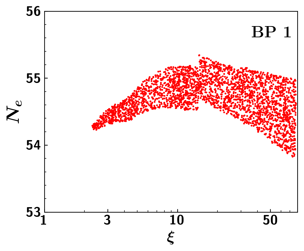
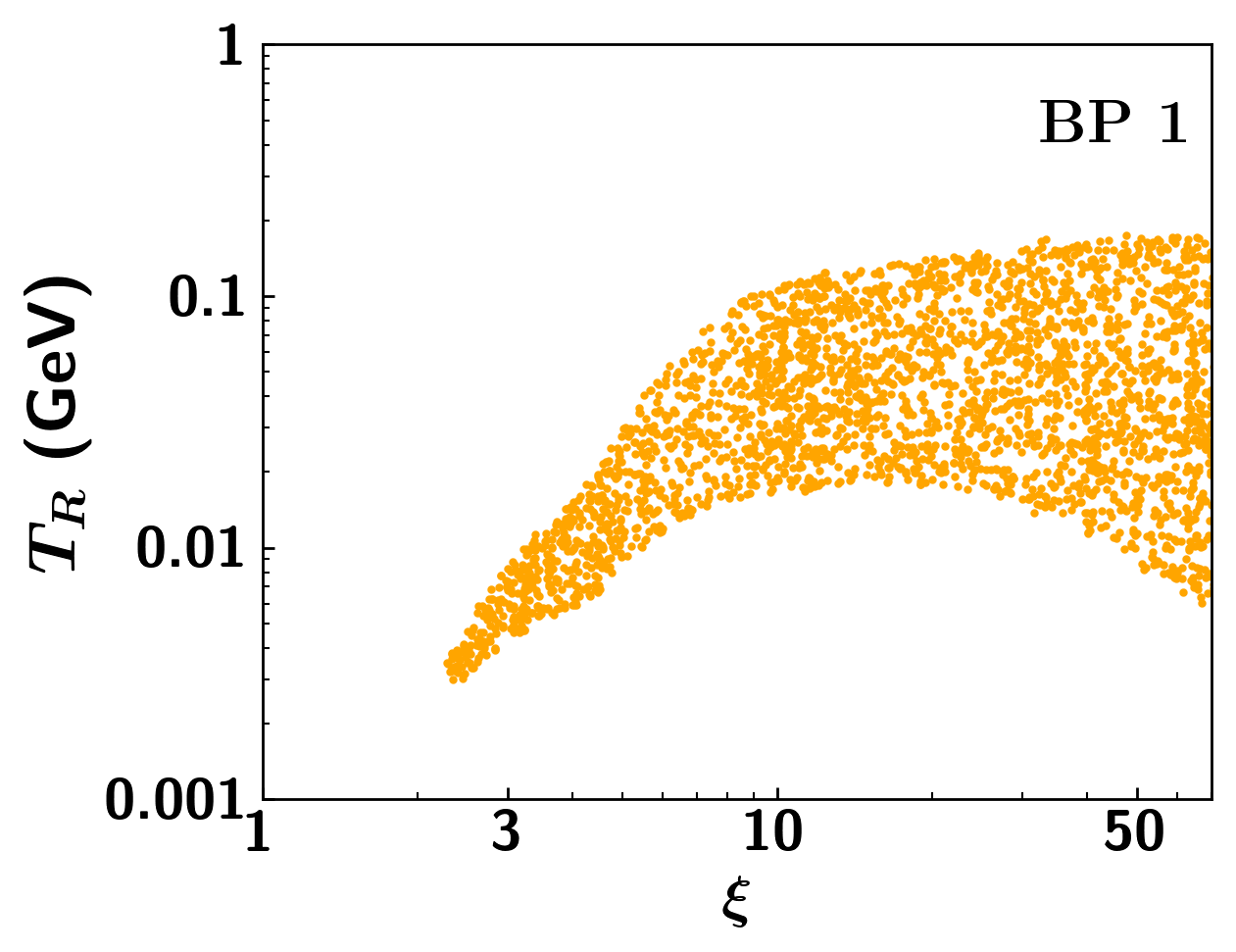
Figure 5: The allowed regions satisfying the constraints on scalar sector parameters (see Fig. 4) are shown in (left) $\xi-N_{\rm e}$ plane and (right) $\xi-T_{\rm RH}$ plane.

Figure 6: The allowed region (white) in the $n_{s}-r$ plane satisfying the constraints on the scalar sector parameters as shown in Fig. 4. The color codes are kept same as in Fig. 4. The region below the solid brown line corresponds to $\xi>80$ where $m_{\phi}>m_{Z^{\prime}}$.

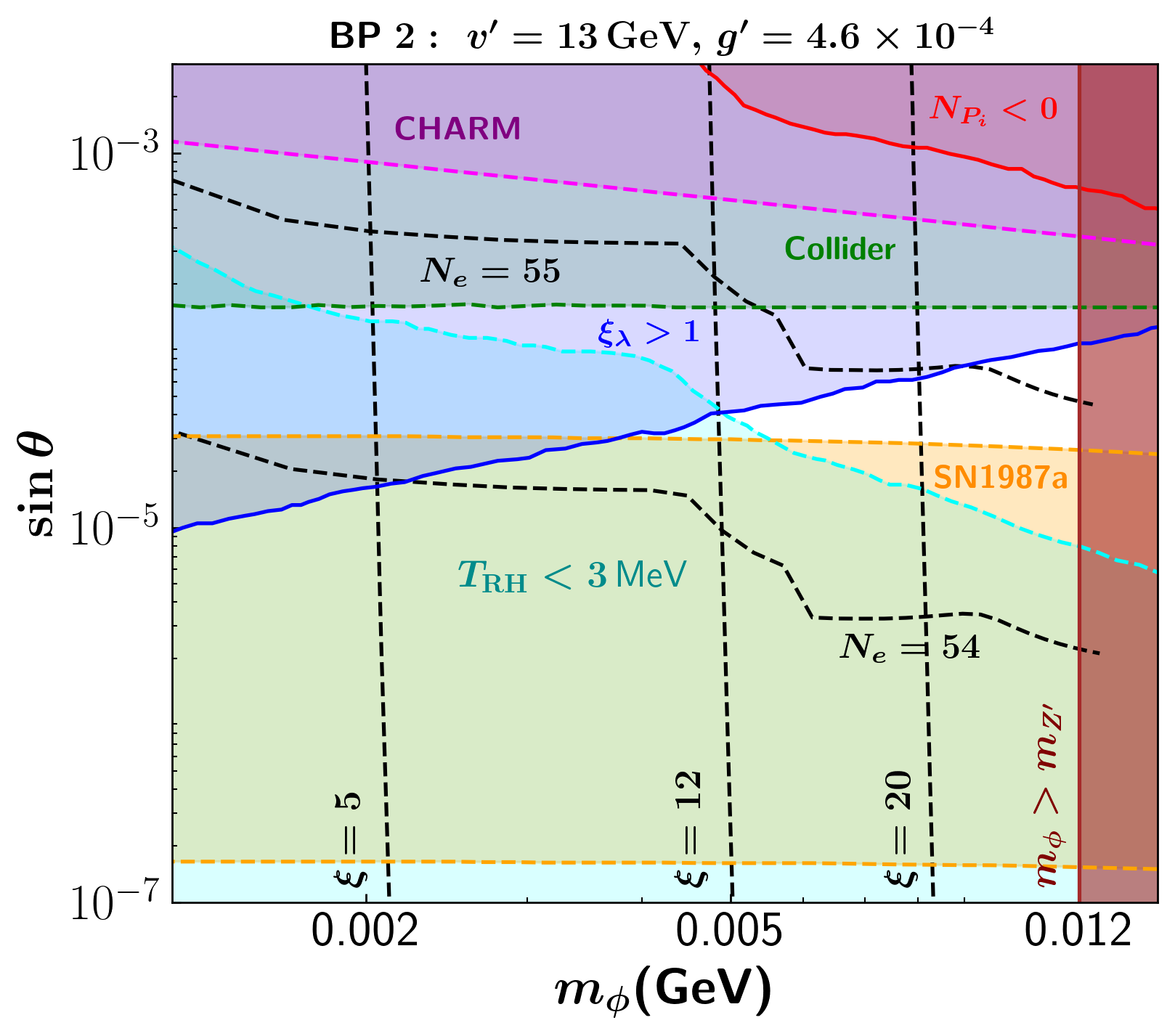
Figure 7: This plot bears same information as Fig. 4, but for BP 2.

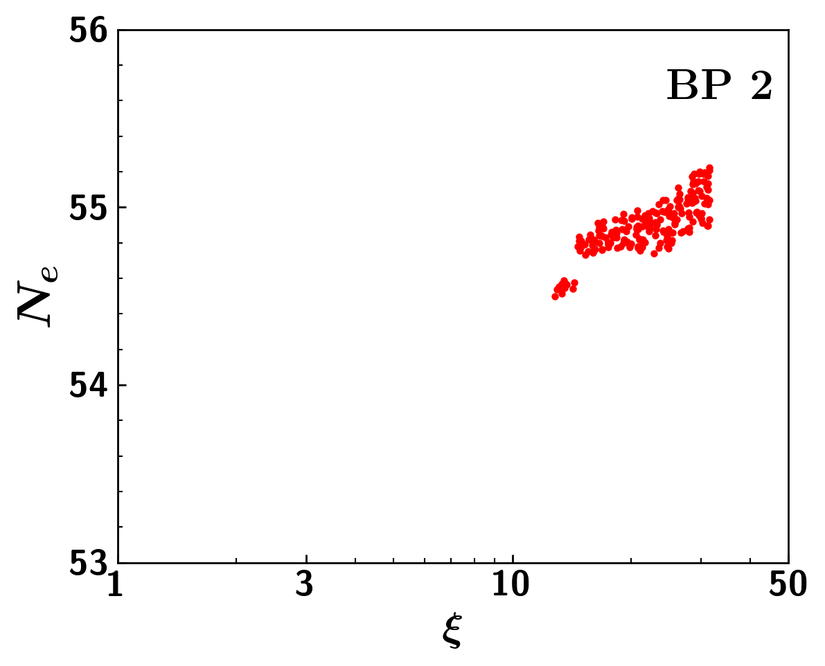
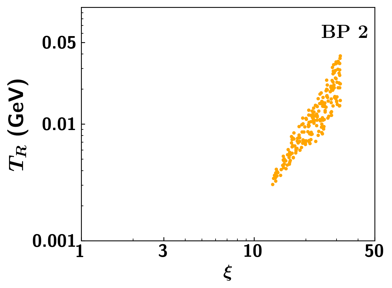
Figure 8: The plots of the top panel bear same information as Fig. 5: left and right panel respectively, however for BP 2. The bottom panel shows the allowed region of $n_{s}-r$ plane for BP 2.

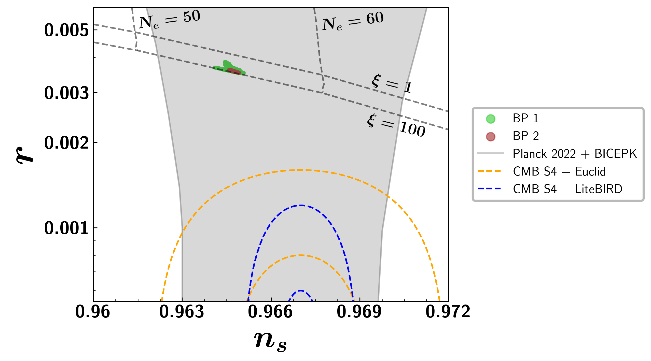
Figure 9: $n_{s}-r$ predictions for BP 1 (green) and BP 2 (brown) in Fig. 2. The Planck+BICEPK Akrami et al. (2020); Ade et al. (2022) 1-$\sigma$ allowed region is indicated by gray. Blue and orange contours correspond to 1-$\sigma$ (dashed) and 2-$\sigma$ (dotted) future sensitivites of CMB S4 Abazajian et al. (2022)+Euclid Laureijs et al. (2011) and CMB S4+LiteBIRD Allys et al. (2023) respectively assuming mean value of $n_{s}=0.967$ and $r=0$. The gray dashed and dotted lines are the estimates of $n_{s}-r$ corresponding to a generic non-minimal quartic inflation model.

We assume the transitions from one phase to another (e.g. radiation-matter crossover during inflaton oscillations) in this calculation as instantaneous. It is also possible that the gauge coupling $g^{\prime}$ can give rise to energy drain of inflaton into radiation via preheating mechanism well before the instantaneous perturbative reheating. We have checked numerically that even if the energy transfer is sizeable during preheating epoch, our results does not change considerably (see appendix. A for details). In fact, the preheating solely is unable to drain the total energy density out of the inflaton field as observed from rigorous lattice simulation Podolsky et al. (2006); Bernal et al. (2018); Maity and Saha (2019). This fact upholds the utmost necessity of efficient perturbative reheating via inflaton decay to set the correct initial conditions for the big bang nucleosynthesis.

V Results

In the preceding section we have explained how a fixed number of inflationary e-foldings can provide us an estimate of $T_{\rm RH}$. At the same time, $T_{\rm RH}$ is also a function of the scalar sector parameters ($m_{\phi},~{}\sin\theta$). This connection allows us to find a correlation between the set of parameters: ($\xi,~{}N_{\rm e}$) and $(m_{\phi},~{}\sin\theta)$ as shown in Fig. 4. Recall that to satisfy the $(g-2)_{\mu}$ results, $v^{\prime}$ is strictly restricted to remain in the range $13{\,\rm GeV}\lesssim v^{\prime}\lesssim 75{\rm\,GeV}$. Note that the $L_{\mu}-L_{\tau}$ gauge coupling $g^{\prime}$ does not have any direct impact on the predictions for inflationary observables. However since we are working in the $m_{\phi}<m_{Z^{\prime}}$ regime, the chosen value of $g^{\prime}$ sets the maximum allowed value of $\xi$ for a particular $v^{\prime}$ as we will see in a while.

For the purpose of numerical analysis, we have considered two benchmark points [BP 1]: $v^{\prime}=75\,{\rm GeV},\,g^{\prime}=1.2\times 10^{-3}$ and [BP 2]: $v^{\prime}=13\,{\rm GeV},\,g^{\prime}=4.6\times 10^{-4}$. These BPs represent the largest and smallest allowed value of $m_{Z^{\prime}}$ and $g^{\prime}$, consistent with the $(g-2)_{\mu}$ data as well other relevant experimental constraints as evident from Fig. 2.

In Fig. 4, we mark different constant $\xi$ and $N_{\rm e}$ lines in the $m_{\phi}-\sin\theta$ plane considering BP 1. This figure reveals that a particular set of $(\xi,N_{\rm e})$ corresponds to a distinct set of ($m_{\phi},\sin\theta$) values. For sub-MeV $m_{\phi}$, the $m_{\phi}-\sin\theta$ plane is restricted from different experiments, namely CHARM Bergsma et al. (1985), SN1987a Dev et al. (2020a); Krnjaic (2016) and colliders Balaji et al. (2022); Dev et al. (2017); Egana-Ugrinovic et al. (2020); Dev et al. (2020b). In addition, we impose a few other important constraints related to inflaton field dynamics in the same plane which are,

• $T_{\rm RH}\gtrsim 3$ MeV, as required to satisfy the BBN constraints.

• $\xi\lesssim 80$, this choice of not so large non-minimal coupling $\xi$ translates into $m_{\phi}<m_{Z^{\prime}}$. This subsequently blocks the decay processes $\phi\to Z^{\prime}+2f$ and $2Z^{\prime}$ at tree level.

• $\xi_{\lambda}\lesssim 1$ (with $\lambda_{H\phi}=\sqrt{4\xi_{\lambda}\lambda_{H}\lambda_{\phi}}$), this ensures that the scalar sector couplings $\lambda_{H}$ and $\lambda_{H\phi}$ do not provide significant corrections to the inflaton potential and also assures its stability Okada and Raut (2017).

• The respective durations during the oscillation regime of inflaton, expressed in terms of quantities $N_{rad}={\rm ln}\left(\frac{a_{\phi,\rm matter}}{a_{\phi,{\rm rad}}}\right)$ and $N_{\rm matter}={\rm ln}\left(\frac{a_{\rm RH}}{a_{\phi,\rm matter}}\right)$ have to be positive in magnitude.

After imposing all these constraints in $m_{\phi}$ - $\sin\theta$ plane, it is realised that the amount of e-foldings during inflation cannot be arbitrary for a fixed $\xi\,(\lesssim 80)$. This is clearly depicted in the left panel of Fig. 5 where the allowed range for $N_{\rm e}$ is plotted as a function of $\xi$. In the same line, these observations also set the allowed ranges for the $T_{\rm RH}$ as a function of $\xi$ as shown in right panel of Fig. 5. As a numerical example, for $\xi=10$, we find $54.5\lesssim N_{\rm e}\lesssim 55.3$ and $20{\rm\,MeV}\lesssim T_{\rm RH}\lesssim 100{\rm\,MeV}$. Once we have obtained the allowed range for $N_{\rm e}$ as a function of $\xi$, next we proceed to estimate the values of spectral index and tensor to scalar ratio. We present our findings in Fig. 6. The different shaded regions (above the solid brown line) are disfavored from the relevant constraints as portrayed earlier in the $m_{\phi}$ - $\sin\theta$ plane of Fig. 4 with the same color codes. The region below the solid brown line corresponds $\xi>80$ and hence our choice $m_{\phi}<m_{z^{\prime}}$ breaks down. We end up with a small white region in the $n_{s}-r$ plane which corresponds to the predictions for $n_{s}$ - $r$ for BP 1. Next we portray the results for BP 2 in Fig. 7 and 8. Following a similar approach used for BP 1 we show the allowed ranges of $N_{\rm e}$, $T_{\rm RH}$ in the top panel of Fig. 8. Next, we provide the $n_{s}$ - $r$ predictions corresponding to BP 2 in the bottom panel of Fig. 8.

Finally, we highlight our findings of $n_{s}-r$ against the existing Planck data as well as future observations from CMB S4 Abazajian et al. (2022) and LiteBIRD Allys et al. (2023) etc. experiments in Fig. 9. For comparison purpose, we also provide the $n_{s}-r$ values corresponding to a generic non-minimal quartic inflation for $\xi=1$ and 100 as indicated by dotted lines. As observed, the $n_{s}-r$ predictions for both BP 1 and BP 2 are much more restricted than the one in non-minimal quartic inflation due to the involvement of $(g-2)_{\mu}$ data in combination with all other relevant theoretical and experimental constraints in the $m_{Z^{\prime}}-g^{\prime}$ and $m_{\phi}-\sin\theta$ planes. It is also noticed that $n_{s}-r$ values corresponding to BP 2 is a subset of the one corresponding to BP 1. We have also confirmed that for any random benchmark point in the $m_{Z^{\prime}}-g^{\prime}$ plane (Fig. 2), the obtained estimates of $n_{s}-r$ always remain inside the predicted region for BP 1 and therefore we conclude that $(g-2)_{\mu}$ data in the minimal $L_{\mu}-L_{\tau}$ model can at most allow $0.964\lesssim n_{s}\lesssim 0.965$ with $0.0035\lesssim r\lesssim 0.0039$. Future CMB experiments like CMB S4 Abazajian et al. (2022) and LiteBIRD Allys et al. (2023) etc. will decide the fate of viability of cosmic inflation in the minimal $L_{\mu}-L_{\tau}$ model accommodating the $(g-2)_{\mu}$ data.

VI Conclusion and Discussions

In this work, we analyse the compatibility of minimal gauged $L_{\mu}-L_{\tau}$ model in accommodating cosmic inflation, consistent with the $(g-2)_{\mu}$ data. We identify the additional SM gauge singlet scalar as the inflaton which is non-minimally coupled with the gravity. We observe that satisfaction of $(g-2)_{\mu}$, consistent with the other existing experimental constraints set the preferred range for the vev of the additional scalar. The non-zero vev of the scalar has two fold non-trivial roles in the post inflationary evolution of the Universe. First of all, $v^{\prime}$ determines the shape of the inflaton potential at low field values, relevant for inflaton oscillation. Secondly, $v^{\prime}$ enters into the mass parameter of inflaton which along with the Higgs portal coupling controls the reheating temperature of the Universe. Note that the $m_{\phi}-\sin\theta$ plane is severely restricted by different theoretical and experimental constraints in the sub-GeV inflaton mass regime.

On another front a viable cosmological history of the Universe uniquely predicts the reheating temperature of the Universe for a given inflationary number of e-folds. This after taking into account the phenomenological constraints in the $m_{\phi}-\sin\theta$ plane significantly constrains the allowed reheating temperature of the Universe and also the number of inflationary e-folds. Using the bound on inflationary number of e-folds we further compute the spectral index and tensor to scalar ratio. We find satisfaction of $(g-2)_{\mu}$ data allows $n_{s}$ and $r$ to remain in a very narrow region compared to the ones in a generic non-minimal quartic inflationary set up and is refutable by future CMB experiments with improved sensitivities.

VII Acknowledgements

AP acknowledges Deep Ghosh and Sk Jeesun for useful discussions and several comments. AP thanks IACS, Kolkata for financial support through Research Associateship. AKS is supported by a postdoctoral fellowship at IOP, Bhubaneswar, India. A.K.S. would like to acknowledge NPDF grant PDF/2020/000797 from the SERB, Government of India, during his stay at IACS where this work was initiated.

Appendix A Comment on preheating

In this work we have assumed that the energy density is stored in the inflaton zero momentum mode until it dissipates into radiation at the reheating epoch. However, realistically, during the initial oscillations of the inflaton (much before the perturbative reheating takes place) a fraction of the energy is dissipated both into higher momentum modes of inflaton and to other fields coupled to the inflaton. This process is known as preheating. The dissipation of inflaton energy through preheating results into a relatively longer or shorter radiation like period (from $a_{\phi,\rm rad}$ to $a_{\phi,\rm matter}$) before the matter like oscillation of the inflaton dominates, thereby slightly increasing or decreasing the ratio $\frac{a_{\phi,\rm matter}}{a_{\phi,\rm rad}}$ which we denote by $\exp(\Delta N)$.

If at the end of preheating, $f$ fraction of the total energy density is in the radiation sector, $f=\frac{\rho_{r}}{\rho_{r}+\rho_{\rm inf_{0}}}$ where $\rho_{\rm inf_{0}}$ is the energy density of zeroth mode of inflaton at the end inflation. The it is simple to show that there is a change of e-folding number of radiation-like phase by an amount,

$$\Delta N=\begin{cases}-\frac{1}{4}\log\frac{1}{1-f}\,,&f\lesssim 0.5\\ -\frac{1}{4}\log(2)+\frac{3}{4}\log(\frac{f}{1-f})\,,&f>0.5\end{cases}$$ (17)

As a representative choice of $f=90\%$, we find a small shift in the inflationary e-fold number $N_{e}$ (i.e. $\Delta N_{e}\sim$ 0.5) for a particular set of $(m_{\phi},\sin\theta)$ corresponding to a constant $\xi$ value. This however does not alter the predicted region (Fig. 9) for BP 1 and BP 2 in the $n_{s}-r$ plane at a noticeable amount. Thus we conclude that even if during preheating, a large fraction of the inflaton energy density gets transferred to the radiation at very early stage of inflaton oscillations, our results remain more or less same.

References

- Bennett et al. (2006) G. W. Bennett et al. (Muon g-2), Phys. Rev. D 73, 072003 (2006), arXiv:hep-ex/0602035 .
- Abi et al. (2021) B. Abi et al. (Muon g-2), Phys. Rev. Lett. 126, 141801 (2021), arXiv:2104.03281 [hep-ex] .
- (3) MUON G-2 collaboration, FERMILAB, August 10, 2023 , Talk:New results from the Muon g-2 experiment at Fermilab .
- Aoyama et al. (2020) T. Aoyama et al., Phys. Rept. 887, 1 (2020), arXiv:2006.04822 [hep-ph] .
- Borsanyi et al. (2021) S. Borsanyi et al., Nature 593, 51 (2021), arXiv:2002.12347 [hep-lat] .
- He et al. (1991a) X. G. He, G. C. Joshi, H. Lew, and R. R. Volkas, Phys. Rev. D 43, 22 (1991a).
- He et al. (1991b) X.-G. He, G. C. Joshi, H. Lew, and R. R. Volkas, Phys. Rev. D 44, 2118 (1991b).
- Baek et al. (2001) S. Baek, N. G. Deshpande, X. G. He, and P. Ko, Phys. Rev. D 64, 055006 (2001), arXiv:hep-ph/0104141 .
- Ma et al. (2002) E. Ma, D. P. Roy, and S. Roy, Phys. Lett. B 525, 101 (2002), arXiv:hep-ph/0110146 .
- Baek (2016) S. Baek, Phys. Lett. B 756, 1 (2016), arXiv:1510.02168 [hep-ph] .
- Heeck and Rodejohann (2011) J. Heeck and W. Rodejohann, Phys. Rev. D 84, 075007 (2011), arXiv:1107.5238 [hep-ph] .
- Banerjee et al. (2021) H. Banerjee, B. Dutta, and S. Roy, JHEP 03, 211 (2021), arXiv:2011.05083 [hep-ph] .
- Asai et al. (2017) K. Asai, K. Hamaguchi, and N. Nagata, Eur. Phys. J. C 77, 763 (2017), arXiv:1705.00419 [hep-ph] .
- Guth (1987) A. H. Guth, Adv. Ser. Astrophys. Cosmol. 3, 139 (1987).
- Linde (1987) A. D. Linde, Adv. Ser. Astrophys. Cosmol. 3, 149 (1987).
- Starobinsky (1980) A. A. Starobinsky, Phys. Lett. B 91, 99 (1980).
- Albrecht and Steinhardt (1982) A. Albrecht and P. J. Steinhardt, Phys. Rev. Lett. 48, 1220 (1982).
- Bezrukov (2013) F. Bezrukov, Class. Quant. Grav. 30, 214001 (2013), arXiv:1307.0708 [hep-ph] .
- Bezrukov and Shaposhnikov (2008) F. L. Bezrukov and M. Shaposhnikov, Phys. Lett. B 659, 703 (2008), arXiv:0710.3755 [hep-th] .
- Barbon and Espinosa (2009) J. L. F. Barbon and J. R. Espinosa, Phys. Rev. D 79, 081302 (2009), arXiv:0903.0355 [hep-ph] .
- Lerner and McDonald (2010) R. N. Lerner and J. McDonald, JCAP 04, 015 (2010), arXiv:0912.5463 [hep-ph] .
- Park and Yamaguchi (2008) S. C. Park and S. Yamaguchi, JCAP 08, 009 (2008), arXiv:0801.1722 [hep-ph] .
- Okada et al. (2010) N. Okada, M. U. Rehman, and Q. Shafi, Phys. Rev. D 82, 043502 (2010), arXiv:1005.5161 [hep-ph] .
- Bezrukov and Gorbunov (2013) F. Bezrukov and D. Gorbunov, JHEP 07, 140 (2013), arXiv:1303.4395 [hep-ph] .
- Linde (2015) A. Linde, in 100e Ecole d’Ete de Physique: Post-Planck Cosmology (2015) pp. 231–316, arXiv:1402.0526 [hep-th] .
- Akrami et al. (2020) Y. Akrami et al. (Planck), Astron. Astrophys. 641, A10 (2020), arXiv:1807.06211 [astro-ph.CO] .
- Ade et al. (2022) P. A. R. Ade et al. (Bicep /Keck, Bicep/Keck, BICEP/Keck), Astrophys. J. 927, 77 (2022), arXiv:2110.00482 [astro-ph.IM] .
- Albrecht et al. (1982) A. Albrecht, P. J. Steinhardt, M. S. Turner, and F. Wilczek, Phys. Rev. Lett. 48, 1437 (1982).
- Dolgov and Kirilova (1990) A. D. Dolgov and D. P. Kirilova, Sov. J. Nucl. Phys. 51, 172 (1990).
- Kofman et al. (1994) L. Kofman, A. D. Linde, and A. A. Starobinsky, Phys. Rev. Lett. 73, 3195 (1994), arXiv:hep-th/9405187 .
- Shtanov et al. (1995) Y. Shtanov, J. H. Traschen, and R. H. Brandenberger, Phys. Rev. D 51, 5438 (1995), arXiv:hep-ph/9407247 .
- Liddle and Leach (2003) A. R. Liddle and S. M. Leach, Phys. Rev. D 68, 103503 (2003), arXiv:astro-ph/0305263 .
- Martin and Ringeval (2010) J. Martin and C. Ringeval, Phys. Rev. D 82, 023511 (2010), arXiv:1004.5525 [astro-ph.CO] .
- Drewes et al. (2017) M. Drewes, J. U. Kang, and U. R. Mun, JHEP 11, 072 (2017), arXiv:1708.01197 [astro-ph.CO] .
- Kamada and Yu (2015) A. Kamada and H.-B. Yu, Phys. Rev. D 92, 113004 (2015), arXiv:1504.00711 [hep-ph] .
- Araki et al. (2017) T. Araki, S. Hoshino, T. Ota, J. Sato, and T. Shimomura, Phys. Rev. D 95, 055006 (2017), arXiv:1702.01497 [hep-ph] .
- Lees et al. (2016) J. P. Lees et al. (BaBar), Phys. Rev. D 94, 011102 (2016), arXiv:1606.03501 [hep-ex] .
- Bellini et al. (2014) G. Bellini et al. (Borexino), Phys. Rev. D 89, 112007 (2014), arXiv:1308.0443 [hep-ex] .
- Mishra et al. (1991) S. R. Mishra et al., Phys. Rev. Lett. 66, 3117 (1991).
- Krnjaic et al. (2020) G. Krnjaic, G. Marques-Tavares, D. Redigolo, and K. Tobioka, Phys. Rev. Lett. 124, 041802 (2020), arXiv:1902.07715 [hep-ph] .
- Aggarwal et al. (2022) L. Aggarwal et al. (Belle-II), (2022), arXiv:2207.06307 [hep-ex] .
- Linde (1983) A. D. Linde, Phys. Lett. B 129, 177 (1983).
- Okada and Raut (2017) N. Okada and D. Raut, Phys. Rev. D 95, 035035 (2017), arXiv:1610.09362 [hep-ph] .
- Bergsma et al. (1985) F. Bergsma et al., Physics Letters B 157, 458 (1985).
- Dev et al. (2020a) P. S. B. Dev, R. N. Mohapatra, and Y. Zhang, JCAP 08, 003 (2020a), [Erratum: JCAP 11, E01 (2020)], arXiv:2005.00490 [hep-ph] .
- Krnjaic (2016) G. Krnjaic, Phys. Rev. D 94, 073009 (2016), arXiv:1512.04119 [hep-ph] .
- Balaji et al. (2022) S. Balaji, P. S. B. Dev, J. Silk, and Y. Zhang, JCAP 12, 024 (2022), arXiv:2205.01669 [hep-ph] .
- Dev et al. (2017) P. S. B. Dev, R. N. Mohapatra, and Y. Zhang, Nucl. Phys. B 923, 179 (2017), arXiv:1703.02471 [hep-ph] .
- Egana-Ugrinovic et al. (2020) D. Egana-Ugrinovic, S. Homiller, and P. Meade, Phys. Rev. Lett. 124, 191801 (2020), arXiv:1911.10203 [hep-ph] .
- Dev et al. (2020b) P. S. B. Dev, R. N. Mohapatra, and Y. Zhang, Phys. Rev. D 101, 075014 (2020b), arXiv:1911.12334 [hep-ph] .
- Abazajian et al. (2022) K. Abazajian et al. (CMB-S4), Astrophys. J. 926, 54 (2022), arXiv:2008.12619 [astro-ph.CO] .
- Laureijs et al. (2011) R. Laureijs et al., “Euclid definition study report,” (2011), arXiv:1110.3193 [astro-ph.CO] .
- Allys et al. (2023) E. Allys et al. (LiteBIRD), PTEP 2023, 042F01 (2023), arXiv:2202.02773 [astro-ph.IM] .
- Podolsky et al. (2006) D. I. Podolsky, G. N. Felder, L. Kofman, and M. Peloso, Phys. Rev. D 73, 023501 (2006), arXiv:hep-ph/0507096 .
- Bernal et al. (2018) N. Bernal, A. Chatterjee, and A. Paul, JCAP 12, 020 (2018), arXiv:1809.02338 [hep-ph] .
- Maity and Saha (2019) D. Maity and P. Saha, JCAP 07, 018 (2019), arXiv:1811.11173 [astro-ph.CO] .