Observation of Topological Weyl Type I-II Transition in Synthetic Mechanical Lattices

Abstract

Weyl points are three-dimensional linear points between bands that exhibit unique stability to perturbations and are accompanied by topologically non-trivial surface states. However, the discovery and control of Weyl points in nature poses significant challenges. While recent advances have allowed for engineering Weyl points in photonic crystals and metamaterials, the topological transition between Weyl semimetals with distinct types of Weyl points remains yet to be reported. Here, exploiting the flexible measurement-feedback control of synthetic mechanical systems, we experimentally simulate Weyl semimetals and observe for the first time the transition between states with type-I and type-II Weyl points. We directly observe the change in the band structures accompanying the transition, and identify the Fermi arc surface states connecting the Weyl points. Further, making use of the non-reciprocal feedback control, we demonstrate that the introduction of non-Hermiticity significantly impacts the topological transition point, as well as the edge localization of the Fermi arc surface states. Our findings offer valuable insights into the design and realization of Weyl points in mechanical systems, providing a promising avenue for exploring novel topological phenomena in non-Hermitian physics.

Introduction.$-$ In recent years, topological phenomena have received considerable attention in the field of photonics and phononics systems due to their potential ability to support robust transport against perturbation [1, 2, 3, 4]. A particularly significant model in three dimensions (3D) is that of Weyl semimetals [5, 6], which feature Weyl points (WPs) as linear degeneracies in the band structure. WPs exhibit chiral properties, acting as “sources” or “sinks” of Berry flux carrying opposite topological charges. The topological protection associated with WPs gives rise to intriguing surface states known as “Fermi arcs” in solid-state materials [7, 8]. These WPs have been linked to various fascinating phenomena, including chiral anomalies [9, 10], unconventional superconductivity [11, 12], and large-volume single-mode lasing [13]. There are two distinct types of WPs: Type-I WPs (WP1) possess a standard cone-like energy spectrum with a point-like Fermi surface, while Type-II WPs (WP2) feature a tilted spectrum with two bands touching at the intersection of electron and hole pockets [14]. While different types of WPs feature distinct transport and chiral anomalies [15, 16, 17], for a given material, the type of WPs is usually fixed due to the difficulty in varying the lattice structure [18, 19, 20, 21, 22]. This raises the question of whether we can arbitrarily control and design a fixed lattice structure that can support both types of WPs so that the transition in between can be systematically investigated. Toward this goal, synthetic matter is a promising avenue, where the flexible control parameters not only offer versatile means of manipulation but can serve as synthetic dimensions and provide access to complicated lattice designs [23, 24, 25, 26, 27, 28, 29, 30, 31].

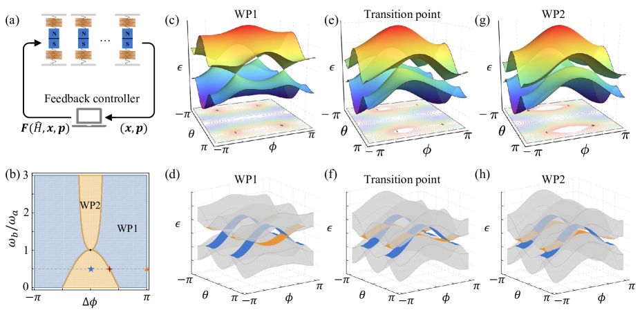
Figure 1: Schematic diagram of experimental mechanical lattices and corresponding Weyl type I-II band structure. (a) Schematic of the mechanical system based on measurements and feedback forces, where each mechanical oscillator (a mass held between two springs) is equipped with embedded accelerometers for the real-time measurement of the position ($x_{i}$) and momentum ($p_{i}$), and a dipole magnet embedded within an anti-Helmholtz coil pair for the application of real-time feedback forces that are used to implement the target Hamiltonian $\hat{H}$. (b) Phase diagram for WP1 and WP2 as a function of modulation phase difference $\Delta\phi$ and detuning frequency ratio $\omega_{b}/\omega_{a}$. (c) Band structure of Weyl type-I for periodic mechanical arrays, corresponding to the orange triangle marked in (b) with $\Delta\phi=\pi$ and $\omega_{b}/\omega_{a}=1/2$. The isoenergy contours of the lower band are shown at the bottom of each figure, where we marked the position and chirality of four WPs with signs “$+$” and “$-$”. (d) The corresponding Weyl Type-I band structure for truncated mechanical arrays, showing the bulk states (transparent grey) and Fermi arc surface states (blue and orange colors marking the top and bottom edges). (e,f) Band structure at Type I-II transition point [at the red cross of (b)]. (g,h) Type II Weyl band structure at the blue star of (b). In all plots, we take $v_{1}=v_{2}=2j$, $\omega_{a}=1.5j$, $k=0$.

Here, we utilize mechanical oscillators to experimentally achieve flexible control over WPs in synthetic dimensions. To generate WPs in three dimensions, we employ measurement-based feedback on mechanical oscillators to construct two additional parametric dimensions in 1D mechanical arrays. By exploiting flexible parametric control, we experimentally observe, for the first time, the transition between states with WP1 and WP2. We characterize the transition through: i) direct detection of the band structure by Fourier-transformed nonequilibrium dynamics; ii) direct detection of the Fermi arc surface states under open boundaries. A unique feature of our mechanical system is its easy access to non-reciprocal feedback control, which can have significant impacts on the topological transitions through the non-Hermitian skin effect (NHSE). We show that both the topological phase transition point and the edge localization of the Fermi arc surface states are tunable through the non-reciprocal coupling. As such, our work sheds new light on the interplay between Weyl phase transition and non-Hermitian physics.

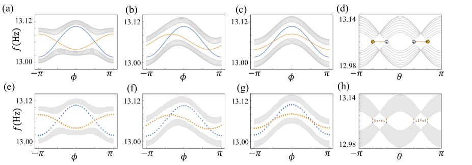
Figure 2: Observation of Weyl type I-II transition and Fermi arcs by band structure measurements. (a-d) Numerically calculated projected band structure at $\theta$ and $\phi$ cut in truncated mechanical arrays, showing the case of Weyl type-I (a), the transition point (b), and Weyl type-II (c) at nontrivial cuts with $\theta=0.45\pi$. (d) The projected WP1 band structure dependence on $\theta$ at a special cut of $\phi=\pi/2$ passing through WPs, where the two edge states appear as arcs connecting a pair of WPs with different chiralities. (e-h) The corresponding projected band structures as measured in experiment (as described in the text). Here we take $v_{1}/2\pi=v_{2}/2\pi=60$ mHz, $j/2\pi=30$ mHz, $\omega_{a}/2\pi=45$ mHz, $\omega_{b}/2\pi=22.5$ mHz, and $2N=18$. The experimental error bars for the edge mode frequencies (typically smaller than the data points) are the standard error based on five measurements.

System description.$-$ To implement flexible parametric control in experiments, we construct a mechanical lattice via measurement-based feedback. The essential idea of this scheme is to map the Heisenberg equations for a desired quantum Hamiltonian onto Newton’s equations of motion for classical oscillators in phase space. (see details in Appendix. A). Briefly speaking, we introduce the classical complex variables $\alpha_{i}=\sqrt{\omega/2}X_{i}+i\sqrt{1/2\omega}P_{i}$ in analogy with the annihilation operator of the quantum harmonic oscillator. To implement Hamiltonian $\hat{H}$, we apply individual feedback forces to the oscillators that are determined by target Hamiltonian and real-time measurement of the position and momentum of oscillators, taking the following form $\mathbf{F}=[f_{1},f_{2},\cdots,f_{n}]^{T}$, $\mathbf{x}=[x_{1},x_{2},\cdots,x_{n}]^{T}$, and $\mathbf{p}=[p_{1},p_{2},\cdots,p_{n}]^{T}$, as shown in Fig. 1(a). These feedback forces can be flexibly controlled, thereby enabling arbitrarily long-ranged or spatially-structured Hamiltonian engineering. The nonequilibrium energy dynamics of the oscillators reflect the eigenstates and energy spectrum of the target Hamiltonian, where the energy distribution plays a role analogous to the local particle probability density $\left|\psi_{i}\right|^{2}$ of a wave function and the energy spectrum can be directly obtained by Fourier transform of the measured $x_{i}(t)$ data. Here, we use self- and cross-feedback between the oscillators. Self-feedback forces proportional to the oscillator positions allow us to shift their frequencies by $\Delta\omega$ from a nominal starting value of $\omega_{0}/2\pi\approx 13.06~{}\text{Hz}$. Cross-feedback forces related to the nearest oscillators’ positions allow us to introduce independent left-to-right and right-to-left hopping terms, with no intrinsic limitation to reciprocal energy exchange [32]. With this, our Hamiltonian can be engineered in parameter and momentum space as

$$h(\theta,k,\phi)= \begin{pmatrix}\Omega_{a}(\phi)&\Upsilon_{1}(\theta,k)\\ \Upsilon_{2}(\theta,k)&\Omega_{b}(\phi)\end{pmatrix}\ .$$ (1)

Here, the diagonal terms are $\Omega_{a}(\phi)=\omega_{0}+\omega_{a}\rm{cos}\phi$ and $\Omega_{b}(\phi)=\omega_{0}+\omega_{b}\rm{cos}(\phi+\Delta\phi)$, where $\omega_{0}$ represents the on-site natural frequency; $\omega_{a,(b)}$ is the detuning frequency and $\phi$ and $\Delta\phi$ are the parameters that modulate this detuning. The off-diagonal terms are $\Upsilon_{1}(\theta,k)=v_{1}\text{cos}\theta+je^{ik}$ and $\Upsilon_{2}(\theta,k)=v_{2}\text{cos}\theta+je^{-ik}$, where the $v_{1(2)}cos\theta$ and $j$ represent intra- and inter-hopping terms, respectively. The parameter $k$ corresponds to the Bloch wave number in 1D real space. To construct a 3D Weyl Hamiltonian, we can consider $\theta$ and $\phi$ as two additional synthetic dimensions in the parametric space. These dimensions, along with $k$, effectively describe the system as a 3D periodic system. In the case of Hermitian systems (where $v_{1}=v_{2}$), the WPs can be obtained by breaking time-reversal symmetry [$h^{*}(\mathbf{-q})=h(\mathbf{q})$] or parity symmetry [$h(\mathbf{-q})=\sigma_{x}h(\mathbf{q})\sigma_{x}$] through modulating the phase difference $\Delta\phi$ and detuning frequency ratio $\omega_{a}/\omega_{b}$ of our system, where $\mathbf{q}$ in parametric space denotes $(\theta,k,\phi)$ (see details in Appendix B). Assuming a WP is located at ($\theta_{0},k_{0},\phi_{0}$) and near the point are ($\theta_{0}+q_{\theta}$, $k_{0}+q_{k}$, and $\phi_{0}+q_{\phi}$), the Hamiltonian of Eq. (1) in the vicinity of a WP can be expanded as $h_{W}(\mathbf{q})=\epsilon_{0}\sigma_{0}+v_{0}q_{\phi}\sigma_{0}+v_{\theta}q_{\theta}\sigma_{x}+v_{k}q_{k}\sigma_{y}+v_{\phi}q_{\phi}\sigma_{z}$, with $\epsilon_{\pm}(\mathbf{q})=\epsilon_{0}+T\pm U$, where the potential energy $U=\sqrt{v_{\theta}^{2}q_{\theta}^{2}+v_{k}^{2}q_{k}^{2}+v_{\phi}^{2}q_{\phi}^{2}}$ and the kinetic energy $T=v_{0}q_{\phi}$. The condition for a WP to be of type II is that there exists a direction $\mathbf{q}$, for which $T(\mathbf{q})>U(\mathbf{q})$. If such a direction does not exist, the WP is of type I [14].

Fig. 1(b) shows the phase diagram for WP1 and WP2 versus the modulation phase difference $\Delta\phi$ and detuning frequency ratio $\omega_{b}/\omega_{a}$. The phase diagram allows us to precisely determine the boundary where the system undergoes a transition between WP1 and WP2. For each type, there are 8 WPs in the first Brillouin zone. Here we exhibit four WPs in parametric space with $k=0$ (another four are localized at $k=\pi$). For WP1 dominated by potential energy $U$, the band structure exhibits a point-like Fermi surface at the WPs where the isoenergy contour of the band structure is closed and takes the shape of an ellipse, as illustrated in Fig. 1(c). The sign “$+$” or “$-$” at each WP denotes its chirality, which is characterized by the sign of $c=\text{sgn}[\det(v_{\theta}v_{k}v_{\phi})]$ [18]. When open boundary conditions are considered in real space, achieved through truncation in mechanical arrays while maintaining periodic boundary conditions in parameter space, we observe two surface states appear as an open-ended section connecting a pair of WPs, in analogy to the Fermi arc in electronic systems. As we can see from the band structure in Fig. 1(d), the two surface states (shown as blue and orange sheets between the upper and lower bulk modes), which are like stripes, are well separated from bulk states. These surface states intersect to form four arcs that connect four pairs of WPs. For WP2, where $T$ is dominant over $U$, the tilt of the band becomes large enough to produce touching electron and hole pockets, rather than a point-like Fermi surface. As a result, the isoenergy contour is open and hyperbolic in the vicinity of WP2, as shown in Fig. 1(g,h). Differing from WP1 and WP2, the isoenergy contour at the transition point, in Fig. 1(e,f), is a hybrid of hyperbolic and elliptical shapes near type I and II WPs. The clear distinction between the two types of WPs leads to drastic band differences in response to the control parameters, allowing us to observe the type I-II transition in experiments.

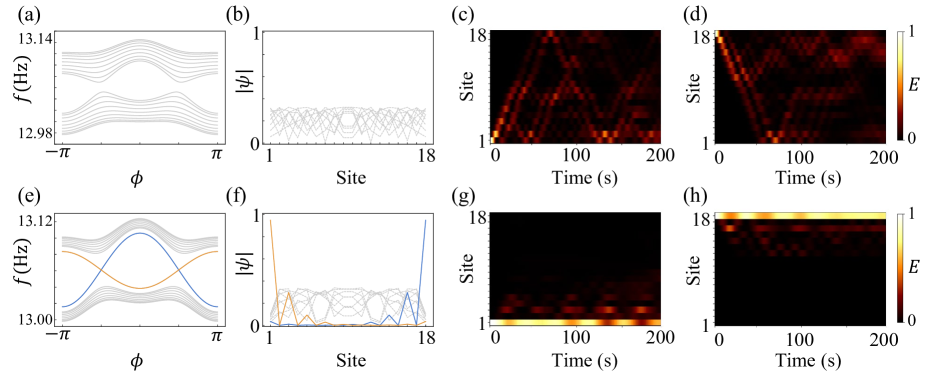
Figure 3: Direct observation of the Fermi arc surface states. (a-b) Numerically calculated band structure in the trivial region with $\theta=0.3\pi$ and the corresponding mode profiles at $\phi=\pi/2$. (c-d) Experimentally observed energy distribution of all oscillators evolving with time, where we initially shake either the first (c) or last (d) oscillator. The brightness in these plots reflects the amount of normalized energy at each oscillator. (e-h) Numerically calculated (e,f) and experimentally observed (g,h) results in the nontrivial region with $\theta=0.45\pi$, showing the presence of edge states. The orange and blue curves represent the two edge states, which intersect and form an open arc between two WPs. Here we exhibit the surface states in the WP1 region ($\Delta\phi=\pi$) and the parameters used in experiments remain consistent with those presented in Fig. 2.

Experimental observation of Weyl type I-II transition and Fermi arc surface states.$-$ In experiments, we can distinguish the WP1 and WP2 by measuring the group velocity in $\phi$ parametric space, which is given by $v_{g,\pm}^{\phi}(q_{\theta},q_{k},q_{\phi})=\partial\epsilon_{\pm}(\mathbf{q})/\partial q_{\phi}$. In the vicinity of WPs with $q_{\theta}=q_{k}=0$, the group velocities can be reduced to $v_{g,\pm}^{\phi}(0,0,q_{\phi})=v_{0}\pm v_{\phi}$. For WP1, the group velocities of the two edge states should have opposite directions [Fig. 2(a)]. On the contrary for Type-II WPs, the two group velocities should have the same directions [2(c)]. And at the transition point, the group velocity satisfies $\left|v_{0}\right|=\left|v_{\phi}\right|$. One of the edge states manifests a flat dispersion relation with vanishing group velocity, as depicted in Fig. 2(b). In experiments, we probe the edge modes by beginning with energy only at either the first or last oscillator positions, while we explore the bulk modes by beginning with energy in the ninth site. By measuring the time evolution of the oscillator dynamics and performing a Fourier transform of the $x_{i}(t)$ signals, we obtain the relevant frequency spectra as shown in Fig. 2(e)-(g). Here, the orange dots are the peaks of the Fourier spectra of $x_{1}(t)$ after initializing at oscillator 1, the blue dots are the peaks of the Fourier spectra of $x_{18}(t)$ after initializing at oscillator 18, and the gray bands are the regions of the Fourier spectra of $x_{j}(t)$ after initializing at inner oscillator $j$ that have weight above a chosen critical value. Additionally, when we measure the projected band structure as a function of $\theta$ along a specific cut that passes through the WPs, we also observe the presence of Fermi arcs that connect a pair of WPs, as demonstrated in Fig. 2(h). This experimental result aligns well with the theoretical predictions shown in Fig. 2(d). Here, each set of data (points/bands) is acquired from five repeated measurements, incorporating small error bars to depict the minor fluctuations observed in the experiments.

Besides measuring the band structure, the Fermi arc surface states can also be probed through the edge dynamics. In the experiments, we initialize energy at the first or last oscillator and then measure the energy transport throughout the lattice. If a surface state is present, the oscillators’ energies should remain relatively confined to the system’s edge, otherwise, it will extend into the bulk. In the trivial region where the parameter $\theta$ is chosen not between two WPs (WPs located at $\theta=\pi/3$ and $2\pi/3$), there is no surface state [Fig. 3(a,b)]. Thus, we find that the initial excitations propagate into the system’s bulk as shown in Fig. 3(c,d). In contrast, in the topologically nontrivial region, where the edge states intersect to form an open arc that connects two WPs [Fig. 3(e,f)], the states can be strongly confined to the initial edge. As shown in Fig. 3(g,h), where the parameter $\theta=0.45\pi$ is chosen between the WPs, the states exhibit strong confinement to the edges, resulting in less penetration depths along the truncated directions.

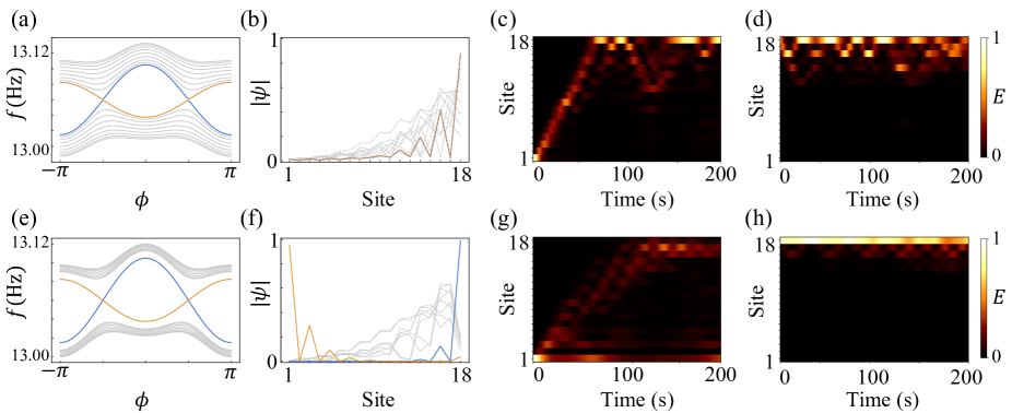
Figure 4: Edge localization transition on Fermi arc from the competition of band topology and non-Hermiticity. We exhibit the numerical band structure, mode profiles, and the experimental time evolution of normalized oscillator energies with $\theta=0.3\pi$ (a-d) and $\theta=0.45\pi$ (e-h), respectively. The surface states exhibit a localization transition, moving from one edge to the opposite edge. While we exhibit the results in the WP1 region, this phenomenon can also be observed in the WP2 region and at the WP1-WP2 transition. In the experiment, we take $v_{1}/2\pi=24$ mHz, $v_{2}/2\pi=60$ mHz, and other parameters remain identical to those depicted in Fig. 3.

Impact of non-reciprocal coupling.$-$ Going further, one advantage of using feedback to engineer Hamiltonians is the straightforward realization of non-reciprocal couplings. Non-reciprocal Hamiltonians naturally host chiral phenomena [33], and can give rise to the intriguing non-Hermitian skin effects [34]. While non-reciprocity would be challenging to access in physical systems governed by Newtonian mechanics – where forces come in equal and opposite pairs – it can effectively be engineered in active matter [35, 36, 37] and in systems featuring dissipation [38]. In our synthetically coupled mechanical lattices, it is possible to engineer non-reciprocity [32, 39]. By applying a non-reciprocal intra-hopping feedback control ($v_{1}\neq v_{2}$ in Eq. (1)), we demonstrate that the non-Hermiticity can impact the Weyl band structure in two ways. First, it extends Weyl points into Weyl rings, and thus modifies the topological transition point for the Weyl semimetal. As depicted in Fig.4(a), surface states appear at $\theta=0.3\pi$, which are absent in the Hermitian case [Fig. 3(a)] (see Fig. 6, Fig. 7 in Appendix for the non-Hermitian ring band structure). Second, it changes the edge localization of the Fermi arc surface states. As shown in Fig. 4(b), both surface states localize on the same side due to NHSE. As a result, illustrated in Fig. 4(c,d), the initially excited energy at the first oscillator exhibits a directional flow for short-time dynamics, and finally tends to the same edge as the case of initially exciting energy at the last oscillator, consistent with the well-known directional current under NHSE. Interestingly, as the non-reciprocal coupling changes, the two surface states on the Fermi arc undergo an edge localization transition and become separately distributed at the two edges [Fig. 4(e,f)]. As demonstrated in Fig. 4(g), the energy initialized at the first oscillator separates into two distinct parts. One tends to flow towards the bulk, displaying a directional flow, and eventually localizes at the upper edge due to NHSE. In contrast, the other part remains localized at the lower edge, together with the excited edge mode seen in Fig. 4(h), revealing existence of two different localized mode distributions. This transition from non-Hermitian skin effect dominance to symmetry dominance is induced by the competition between non-Hermiticity and band topology. In the thermodynamic limit, the transition point occurs at $\mathrm{max}\{|v_{1}\mathrm{cos}\theta|,|v_{2}\mathrm{cos}\theta|\}=|j|$, where the surface states with non-degenerate energies exhibit a completely delocalized distribution (details in Appendix C). This behavior stands in contrast to those observed in the Hermitian region and further reflects the unique localization characteristics and mode propagation behavior exhibited by non-Hermitian systems, which has sparked recent interest [40, 41].

Conclusion.$-$ Our study presents a synthetic 3D Weyl model in a mechanical lattice, which was realized by measurement-based feedback. Through flexible control in parametric space, we successfully observed the transition between WP1 and WP2 and demonstrated the emergence of Fermi-arc states by the observed band structure and edge dynamics in experiments. Furthermore, by implementing non-reciprocal feedback control, we demonstrate that the non-Hermiticity can impact the Weyl band structure in two ways: i) the Fermi arc surface states are extended from connecting two Weyl points to Weyl rings; ii) the edge localization of Fermi arc surface states is modified by the competition between band topology and non-Hermiticity. These exciting findings not only provide the first experimental demonstration of a Weyl type-I and type-II transition but also contribute to the advancement of our understanding of Weyl semimetals in the non-Hermitian region, opening up new avenues for investigating diverse topological phenomena.

Looking forward, there are still many novel topological phenomena to explore in non-Hermitian Weyl physics, for example, the non-Hermitian skin effect can reshape the wavefunctions of surface modes by delocalizing them from the boundary (as seen in Fig. 8), thereby possessing the potential to engineer topological modes into a diversity of shapes in the Weyl bulk lattice, similar to the topological morphing modes in Ref. [40, 41]. What’s more, the flexible control of our systems can also serve as a valuable tool for exploring various physical phenomena related to non-Hermitian topology [42, 43, 44, 45, 46, 47, 48, 49, 50, 51, 52, 53, 54, 55], nonlinear dynamics [56, 57, 58], non-Abelian physics [59], synchronization [60], and discrete classical time crystals [61]. This capability opens up exciting avenues for further exploration and the discovery of new phenomena in diverse fields of research.

Appendix A Experimental implementation

The theoretical basis for our synthetic mechanical lattices is mapping Newton’s equation of motion to the Heisenberg equations for Hamiltonian, as described in Ref. [32]. In this section, we give the theoretical derivation and describe the implementation in our experiments.

The equations of motion for uncoupled and identical harmonic oscillators are:

$$m\dot{x}_{i}(t)=p_{i}(t),\quad\dot{p}_{i}(t)=-m\omega^{2}x_{i}(t),$$ (2)

where $x_{i}(t)$ and $p_{i}(t)$ are position and momentum of $i$th oscillator, $\omega$ is the natural oscillation frequency, and $m$ is the mass. For simplicity, we introduce the notation $X_{i}\equiv-\omega^{2}x_{i}(t)$ and $P_{i}\equiv\frac{-\omega^{2}}{m}p_{i}(t)$, so that the equations of motion become

$$\dot{X}_{i}=P_{i},\quad\dot{P}_{i}=-\omega^{2}X_{i}.$$ (3)

To couple these oscillators as a basis for simulating different Hamiltonians, we now add feedback forces to the system such the equations of motions become

$$\dot{X}_{i}=P_{i},\quad\dot{P}_{i}=-\omega^{2}X_{i}+f_{i}.$$ (4)

where $f_{i}$ is a linear function of $(X_{1},X_{2},\cdots,X_{n},P_{1},P_{2},\cdots,P_{n})$.

To map the above equations to Heisenberg equations, we introduce the classical complex variables:

$$\alpha_{i}\equiv\sqrt{\frac{\omega}{2}}X_{i}+i\sqrt{\frac{1}{2\omega}}P_{i}$$ (5)

in analogy with the annihilation operator of the quantum harmonic oscillator. From this, it follows that

$$X_{i}=\sqrt{\frac{1}{2\omega}}\left(\alpha_{i}+\alpha_{i}^{*}\right),\quad P_{i}=-i\sqrt{\frac{\omega}{2}}\left(\alpha_{i}-\alpha_{i}^{*}\right),$$ (6)

and hence the equations of motion are

$$\dot{\alpha}_{i}=-i\omega\alpha_{i}+\frac{i}{\sqrt{2\omega}}f_{i}=-i\omega\alpha_{i}+\frac{i}{\sqrt{2\omega}}\sum_{j}M_{ij}(\alpha_{j}+\alpha_{j}^{*}).$$ (7)

where the feedback term, $f_{i}$, is expressed as a linear function of $f_{i}=\sum_{j}M_{ij}(\alpha_{j}+\alpha_{j}^{*})$. To note, this form is specific to the implementation of only $X_{j}$-dependent feedback forces, relating to real-valued hopping terms and real site-dependent frequency shifts, as utilized in this work. This equation can be regarded as the Heisenberg equation of motion derived from a quantum mechanical Hamiltonian (with $\hbar=1$):

$$\hat{H}=\sum_{i}\omega\hat{\alpha}_{i}^{\dagger}\hat{\alpha}_{i}-\frac{1}{\sqrt{2\omega}}\sum_{i,j}\hat{\alpha}_{i}^{\dagger}\hat{M}_{ij}(\hat{\alpha}_{j}+\hat{\alpha}_{j}^{\dagger}),$$ (8)

where $\hat{\alpha}_{i}^{\dagger}$ and $\hat{\alpha}_{i}$ are creation and annihilation operators for site $i$ obeying bosonic commutation relations, with $\alpha_{i}=\left\langle\hat{\alpha}_{i}\right\rangle$ and $\alpha_{i}^{*}=\left\langle\hat{\alpha}_{i}^{\dagger}\right\rangle$.

Now, we assume that the feedback is sufficiently weak compared to the natural oscillations. Within this limit, the complex amplitudes’ time-dependence is still given by $\alpha_{i}(t)\propto e^{-i\omega t}$. This allow us to apply the ”rotating-wave approximation” (RWA) to simplify Eq. (9):

$$\hat{H}_{\rm RWA}=\sum_{i}\omega\hat{\alpha}_{i}^{\dagger}\hat{\alpha}_{i}-\frac{1}{\sqrt{2\omega}}\sum_{i,j}\hat{\alpha}_{i}^{\dagger}\hat{M}_{ij}\hat{\alpha}_{j}.$$ (9)

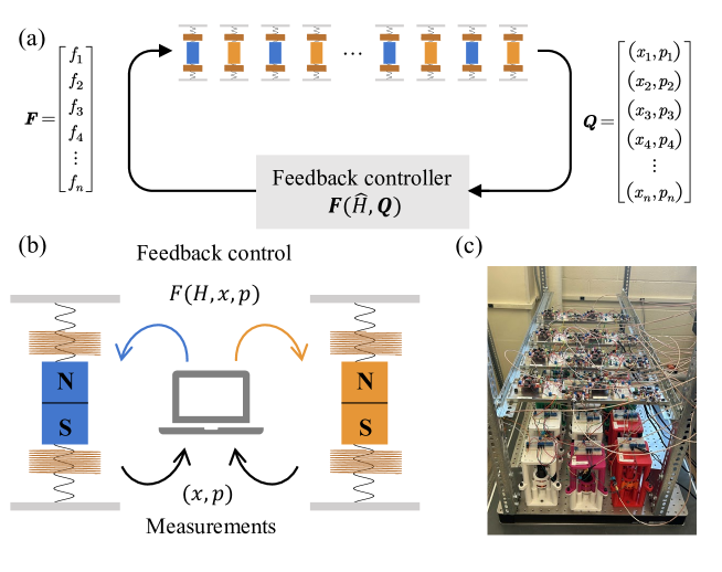
Figure 5: Implementation of our model in a mechanical system via measurement and feedback. (a) Schematic diagrams of our experimental system and approach. The Hamiltonian can be realized through applied forces that are responsive to real-time measurements. (b) A depiction of the implemented mechanical oscillators, which features embedded accelerometers for the real-time measurement of proxies for the position ($x$) and momentum ($p$), a set of two springs and a dipole magnet embedded in a pair of anti-Helmholtz coils for the application of forces. Real-time feedback forces $F$, which depend on the real-time measurements $x_{i}$ and $p_{i}$, are used to implement the target Hamiltonian $H$. (c) A photograph of our main experimental setup supporting 16 oscillators (2 additional oscillators are located on a separate structure).

In experiments, as shown in Fig. 5, our “lattice of synthetically coupled oscillators” consists of modular mechanical oscillators. In the absence of applied feedback forces, these oscillators exhibit nearly identical natural oscillation frequencies, $\omega_{0}/2\pi\sim 13.06\mathrm{~{}Hz}$. Each oscillator is equipped with an analog accelerometer (EVAL-ADXL203). Real-time measurements of acceleration $a(t)$ are obtained by sending the signals to a common computer (via very high-gauge wire connections). Additionally, by numerically differentiating the acquired signal, we obtain real-time measurements of the oscillators’ jerk, $j(t)\equiv\dot{a}(t)$. Because $x(t)\propto a(t)$ and $j(t)\propto p(t)$ for a harmonic oscillator, we treat the $a$ and $j$ signals as proxies for the position $x$ and momentum $p$. We additionally multiply the signals to put them on a common scale, reflecting the equipartition of harmonic oscillators.

In this work, $p$-dependent feedback is only used for one purpose, to cancel the natural damping of each of the individual oscillators. By applying self-feedback terms proportional to the oscillator momenta ($p_{i}$), we cancel the oscillators’ natural damping and explore coherent dynamics for well over 500 s ($>6500$ periods). These long timescales are essential for achieving the high frequency resolution of the experimental spectra.

We implement the feedback forces magnetically, avoiding any added mechanical contacts. Each oscillator has a dipole magnet attached to a central, cylindrical shaft. The dipole magnet is embedded in a pair of anti-Helmholtz coils. We control the current in these coils, which produces an axial magnetic field gradient that in turn creates a force on the oscillator. We note that we operate the current in a polar fashion, with only one direction of current flow allowed. In the previous iteration of these experiments (Refs. [32, 39]), we controlled positive and negative variations about an overall offset gradient, thus achieving relative bi-directional control of the forces. In this updated iteration, we operate with no current offset, instead simply applying feedback currents only when the oscillating force control signals are determined to be positive (i.e., multiplying by an appropriate Heaviside function). The time-averaged effective feedback is the same, as the reduced duty cycle (forces are only applied for a half of each oscillation period) is compensated by an enlarged dynamic range (as no offset current value is applied), while reducing the power consumption of the experiment.

In terms of our data and its analysis, our primary data consists of the real-time measurements of the ${x}$ and ${p}$ signals for each of the oscillators. From these signals, the energy dynamics as presented in Fig. 3 and Fig. 4 of the main text are determined simply by taking the sum of ${x^{2}}$ and ${p^{2}}$ (having previously scaled these to signals to be on the same footing). We can additionally acquire representative energy spectra for the bulk and edge modes of the system by simply taking a Fourier transform (and plotting its absolute value) of the measured ${x}$ nonequilibrium dynamics signals after applying the appropriate state initialization. As described in the text in relation to Fig. 2, three separate spectra are explored: that of the left edge mode, the right edge mode, and the bulk. The left and right edge modes are explored by initially exciting either the first or last oscillator and then finding the peak of the power spectrum based on the Fourier transform of the $x_{1}(t)$ or $x_{18}(t)$ signals, respectively. For the bulk modes, where more than just the peak of the spectrum is displayed, the gray band regions of Fig. 2 are obtained as follows. We excite only the ninth oscillator from the system bulk and then perform a Fourier transform of the $x_{9}(t)$ dynamics. The gray bands plotted in Fig. 2 represent the regions of the resulting power spectra that have weight above a chosen cutoff value. Each of these three spectra is derived from 500 s of nonequilibrium dynamics after the stated initialization.

Appendix B Weyl Hamiltonian in synthetic systems

Before proceeding, let us first provide an introduction to WPs. WPs in three dimensions exhibit distinct characteristics that set them apart from their two-dimensional counterparts, the Dirac point. The Dirac cone Hamiltonian in 2D has the form of $h(\mathbf{k})=v_{x}k_{x}\sigma_{x}+v_{y}k_{y}\sigma_{y}$, where $v_{i}$ are the group velocities. This form is protected by the product of parity (P) symmetry [$h(\mathbf{k})=\sigma_{x}h(\mathbf{-k})\sigma_{x}$] and time-reversal (T) symmetry [$h^{*}(\mathbf{-k})=h(\mathbf{k})$]. Any perturbation on $\sigma_{z}$ terms, which break P or T, will open a band gap. In comparison, the Weyl Hamiltonian is expressed as $h(\mathbf{k})=v_{x}k_{x}\sigma_{x}+v_{y}k_{y}\sigma_{y}+v_{z}k_{z}\sigma_{z}$. Since all three Pauli matrices are utilized in the Hamiltonian, it becomes impossible to introduce a perturbation that would open a band gap. This unique characteristic ensures the stability and robustness of WPs in 3D periodic systems. The elimination and creation of WPs can only occur through pair-annihilations and pair-generations of WPs with opposite chiralities. These processes typically require a strong perturbation in the system. The chirality ($c=\pm 1$) of a WP can be defined as $c=\text{sgn}(\text{det}[v_{ij}])$ for $h(\mathbf{k})=\sum_{ij}k_{i}v_{ij}\sigma_{j}$ [18].

B.1 Derivation of Weyl Hamiltonian

Our Hamiltonian in real space is:

$$\hat{H}= \sum_{i}^{N}(\omega_{0}+\omega_{a})\text{cos}\phi_{a}~{}\hat{a}_{i}^{\dagger}\hat{a}_{i}+\sum_{i}^{N}(\omega_{0}+\omega_{b})\text{cos}\phi_{b}~{}\hat{b}_{i}^{\dagger}\hat{b}_{i}+\sum_{i}^{N}\left(v_{1}\text{cos}\theta~{}\hat{a}_{i}^{\dagger}\hat{b}_{i}+v_{2}\text{cos}\theta~{}\hat{a}_{i}\hat{b}_{i}^{\dagger}\right)$$ (10)

$$+\sum_{i}^{N-1}\left(j~{}\hat{a}_{i+1}^{\dagger}\hat{b}_{i}+j~{}\hat{a}_{i+1}\hat{b}_{i}^{\dagger}\right),$$

where the first two terms represents on-site terms, including natural frequency $\omega_{0}$, detuning frequency $\omega_{a(b)},$ and modulating terms $\phi_{a}$ and $\phi_{b}$ ($\phi_{a}=\phi$ and $\phi_{b}=\phi_{a}+\Delta_{\phi}$ in the main text). The middle terms $v_{1(2)}\cos\theta$ represent the intra-hopping terms, while the term $j$ corresponds to the inter-hopping terms. Under Fourier transformation, Eq. (10) can be rewritten in momentum space $H=\sum_{k}(\hat{a}^{\dagger}_{k}\,\,\hat{b}^{\dagger}_{k})~{}h(k)~{}(\hat{a}^{\dagger}_{k}\,\,\hat{b}^{\dagger}_{k})^{T}$ with

$$h(k)= \begin{pmatrix}\omega_{0}+\omega_{a}\text{cos}\phi_{a}&v_{1}\text{cos}\theta+je^{ik}\\ v_{2}\text{cos}\theta+je^{-ik}&\omega_{0}+\omega_{b}\text{cos}\phi_{b}\end{pmatrix}$$ (11)

$$= h_{0}\sigma_{0}+h_{x}\sigma_{x}+h_{y}\sigma_{y}+h_{z}\sigma_{z},$$

where $\sigma_{j}$, $j=x,y,z$ is Pauli matrix, and the complex parameter $h_{j}=h_{j}^{R}+ih_{j}^{I}$ takes the form of

$$h_{x}^{R} =\left(v_{1}\text{cos}\theta+v_{2}\text{cos}\theta+2j\text{cos}k\right)/2, h_{x}^{I}=0,$$ (12)

$$h_{y}^{R} =-j\text{sin}k, h_{y}^{I}=\left(v_{1}\text{cos}\theta-v_{2}\text{cos}\theta\right)/2,$$

$$h_{z}^{R} =\left(\omega_{a}\text{cos}\phi_{a}-\omega_{b}\text{cos}\phi_{b}\right)/2, h_{z}^{I}=0,$$

$$h_{0}^{R} =\left(2\omega_{0}+\omega_{a}\text{cos}\phi_{a}+\omega_{b}\text{cos}\phi_{b}\right)/2, h_{0}^{I}=0.$$

The complex-energy spectrum of Eq. (11) can be explicitly expressed as follows

$$E_{\pm}=h_{0}\pm\sqrt{h_{R}^{2}-h_{I}^{2}+2i~{}\mathbf{h_{R}}\cdot\mathbf{h_{I}}},$$ (13)

where $\mathbf{h}=\mathbf{h_{R}}+i~{}\mathbf{h_{I}}$ with $\mathbf{h}\in\mathbb{R}^{3}$.

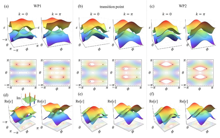
Figure 6: (a-c) Band structure of WP1, transition point, and WP2, where the phase difference satisfies $\Delta\phi=\pi$, $\pi/3$, and $0$, respectively. The corresponding isoenergy contours of the lower band are shown in the second line, where we marked the position and chirality of four WPs with signs “+” and “-”. Here we take $v_{1}=v_{2}=2j$, $\omega_{a}=1.5j$, and $\omega_{b}/\omega_{a}=0.5$. (d-f) The real part of the non-Hermitian band structure, with an inset in (d) displaying the band structure of the imaginary part (the imaginary part band structures in the other figures exhibit the same pattern, hence, for brevity and clarity, we present the results for only one). Here we take non-reciprocal hopping terms satisfying $v_{2}=2.5v_{1}=2j$, and other parameters remain consistent with the Hermitian case.

For the Hermitian case ($v_{1}=v_{2}=v$ with $\mathbf{h_{I}}=0$), degeneracies in the spectrum [Eq. 13] occur only if all three components of $\mathbf{h_{R}}$ are simultaneously tuned to zero. We assume a WP located at ($\theta_{0},k_{0},\phi_{0}$) and near the point are $\theta_{0}+q_{\theta}$, $k_{0}+q_{k}$, and $\phi_{0}+q_{\phi}$. In the vicinity of the WP, the Hamiltonian Eq. (12) should take the Weyl Hamiltonian form [5], and thus can be rewritten as

$$h_{x} =v\text{cos}\theta_{0}+j\text{cos}k_{0}-v\text{sin}\theta_{0}q_{\theta}-j\text{sin}k_{0}q_{k}=v_{\theta}q_{\theta},$$ (14)

$$h_{y} =-j\text{sin}k_{0}+j\text{cos}k_{0}q_{k}=v_{k}q_{k},$$

$$h_{z} =\left(\omega_{A}\text{cos}\phi_{0}-\omega_{B}\text{cos}(\phi_{0}+\Delta\phi\right)/2-\omega_{A}\text{sin}\phi_{0}q_{\phi}/2+\omega_{B}\text{sin}(\phi_{0}+\Delta\phi)q_{\phi}/2=v_{\phi}q_{\phi},$$

$$h_{0} =\left(2\omega_{0}+\omega_{a}\text{cos}\phi_{0}+\omega_{b}\text{cos}(\phi_{0}+\Delta\phi)\right)/2-\omega_{a}\text{sin}\phi_{0}q_{\phi}/2-\omega_{b}\text{sin}(\phi_{0}+\Delta\phi)q_{\phi}/2=\epsilon_{0}+v_{0}q_{\phi},$$

where we set $\Delta\phi=\phi_{b}-\phi_{a}$ and

$$v_{\theta} =-v\text{sin}\theta_{0}, \text{with}\,\text{sin}\theta_{0}=\pm\frac{\sqrt{v^{2}-j^{2}}}{v};$$ (15)

$$v_{k} =j\text{cos}k_{0}, \text{with}\,k_{0}=0,\,\pi;$$

$$v_{\phi} =-\omega_{a}\text{sin}\phi_{0}/2+\omega_{b}\text{sin}(\phi_{0}+\Delta\phi)/2, \text{with}\,\phi_{0}=\pm\text{arccos}\left(\mp\frac{\omega_{b}\text{sin}\Delta\phi}{\sqrt{\omega_{a}^{2}+\omega_{b}^{2}-2\omega_{a}\omega_{b}\text{cos}\Delta\phi}}\right);$$

$$v_{0} =-\omega_{a}\text{sin}\phi_{0}/2-\omega_{b}\text{sin}(\phi_{0}+\Delta\phi)/2, \text{and}\,\epsilon_{0}=\left(2\omega_{0}+\omega_{a}\text{cos}\phi_{0}+\omega_{b}\text{cos}(\phi_{0}+\Delta\phi)\right)/2.$$

The corresponding energy spectrum of the two bands are denoted as follows:

$$\epsilon_{\pm}(\mathbf{q})=\epsilon_{0}+v_{0}q_{\phi}\pm\sqrt{v_{\theta}^{2}q_{\theta}^{2}+v_{k}^{2}q_{k}^{2}+v_{\phi}^{2}q_{\phi}^{2}},$$ (16)

where “+” and “-” correspond to the upper and lower bands, respectively. In order to distinguish between the two types of WPs, we decompose the Hamiltonian (Eq. (12)) into $h_{W}(\mathbf{q})=\epsilon_{0}\sigma_{0}+H_{U}+H_{T}$, with

$$h_{U} =v_{\theta}q_{\theta}\sigma_{x}+v_{k}q_{k}\sigma_{y}+v_{\phi}q_{\phi}\sigma_{z},$$ (17)

$$h_{T} =v_{0}q_{\phi}\sigma_{0},$$

where $h_{U}$ and $h_{T}$ constitute the potential and kinetic energy components of $h_{W}(\mathbf{q})$. The total energy spectra $\epsilon_{\pm}$ can thus be decomposed into the constant energy component of $\epsilon_{0}$ as well as the potential and kinetic energy spectra $U$ and $T$, with

$$U= \sqrt{v_{\theta}^{2}q_{\theta}^{2}+v_{k}^{2}q_{k}^{2}+v_{\phi}^{2}q_{\phi}^{2}};$$ (18)

$$T= v_{0}q_{\phi}.$$

For WP1, $U>T$ should be satisfied in all directions. On the contrary, if there exists a particular direction along which $T$ dominates over $U$ with $T>U$, the WPs are of Type-II. Therefore, the system exhibits a phase transition from WP1 to WP2 at $T=U$. The phase transition point can be obtained by comparing $T$ and $U$. It can also be obtained by measuring the group velocity in $\phi$ parametric space, which is given by

$$v_{g,\pm}^{\phi}(q_{\theta},q_{k},q_{\phi})=\frac{\partial\epsilon_{\pm}(\mathbf{q})}{\partial q_{\phi}}=v_{0}\pm\frac{q_{\phi}v_{\phi}^{2}}{\sqrt{v_{\theta}^{2}q_{\theta}^{2}+v_{k}^{2}q_{k}^{2}+v_{\phi}^{2}q_{\phi}^{2}}}.$$ (19)

In the vicinity of WPs with $q_{\theta}=q_{k}=0$, the group velocities can be reduced to $v_{g,\pm}^{\phi}(0,0,q_{\phi})=v_{0}\pm v_{\phi}.$ For WP1, the group velocities of two bands should have opposite directions, which means $\left|v_{0}\right|<\left|v_{\phi}\right|$. On the contrary for WP2, the two group velocities should have the same direction, such that $\left|v_{0}\right|>\left|v_{\phi}\right|$. So at the phase transition point, the group velocity satisfies $\left|v_{0}\right|=\left|v_{\phi}\right|$. Thus, the two group velocities will become

$$\left\{\begin{array}[]{l}v_{\phi,+}=v_{0}+v_{\phi};\\ v_{\phi,-}=0,\end{array}\right.$$ (20)

showing that one of the bands will become flat in the vicinity of WPs with zero group velocity while the other band has finite group velocity. So the local flat band structure is a physical signature of phase transition occurring at the boundaries between WP1 and WP2. In Fig. 6, we exhibit the projected band structures and isoenergy contours in parametric space with k=0 and k=$\pi$. For each type, there are 8 WPs in the first Brillouin zone.

B.2 Symmetry analysis

Time reversal symmetry requires $h^{*}(\mathbf{-k})=h(\mathbf{k})$, and parity symmetry requires $h(\mathbf{k})=\sigma_{x}h(\mathbf{-k})\sigma_{x}$ in real space with $\mathbf{k}=(k_{x},k_{y},k_{z})$. To analyze the Weyl Hamiltonian symmetry in parametric space, , we replace it with $(k,\theta,\phi)$. In the vicinity of WPs $(k_{0},\theta_{0},\phi_{0})$, we have $(k,\theta,\phi)=(k_{0}+q_{k},\theta_{0}+q_{\theta},\phi_{0}+q_{\phi})$. For time-reversal symmetry, we have

$$h(\theta,k,\phi) =\sigma_{x}q_{\theta}v_{\theta}+\sigma_{y}q_{k}v_{k}+\sigma_{z}q_{\phi}v_{\phi}$$ (21)

$$h^{*}(-\theta,-k,-\phi) =\sigma_{x}q_{\theta}v_{\theta}^{\prime}-\sigma_{y}q_{k}v_{k}^{\prime}+\sigma_{z}q_{\phi}v_{\phi}^{\prime}$$

And time-reversal symmetry [$h^{*}(-\theta,-k,-\phi)=h(\theta,k,\phi)$] requires $v_{\theta}=v_{\theta}^{\prime}$, $v_{k}=-v_{k}^{\prime}$, and $v_{\phi}=v_{\phi}^{\prime}$.

For parity symmetry (inversion symmetry), we have

$$\sigma_{x}h(-\theta,-k,-\phi)\sigma_{x}=\sigma_{x}q_{\theta}v_{\theta}^{\prime}-\sigma_{y}q_{k}v_{k}^{\prime}-\sigma_{z}q_{\phi}v_{k}^{\prime}$$ (22)

and parity symmetry [$\sigma_{x}h(-\theta,-k,-\phi)\sigma_{x}=h(\theta,k,\phi)$] requires $v_{\theta}=v_{\theta}^{\prime}$, $v_{k}=-v_{k}^{\prime}$, and $v_{\phi}=-v_{\phi}^{\prime}$.

For PT symmetry, we have

$$\sigma_{x}h^{*}(-\theta,-k,-\phi)\sigma_{x}=\sigma_{x}q_{\theta}v_{\theta}^{\prime}+\sigma_{y}q_{k}v_{k}^{\prime}-\sigma_{z}q_{\phi}v_{\phi}^{\prime}$$ (23)

and PT symmetry [$\sigma_{x}h^{*}(-\theta,-k,-\phi)\sigma_{x}=h(\theta,k,\phi)$] requires $v_{\theta}=v_{\theta}^{\prime}$, $v_{k}=v_{k}^{\prime}$, and $v_{\phi}=-v_{\phi}^{\prime}$.

In our model, as shown in Eq. (15), we have $v_{\theta}=-v\text{sin}\theta_{0}=v\text{sin}(-\theta_{0})=v_{\theta}^{\prime}$, $v_{k}=j\text{cos}k_{0}=j\text{cos}(-k_{0})=-v_{k}^{\prime}$, $v_{\phi}=-\omega_{a}\text{sin}\phi_{0}/2+\omega_{b}\text{sin}(\phi_{0}+\Delta\phi)/2$, and $v_{\phi}^{\prime}=\omega_{a}\text{sin}(-\phi_{0})/2-\omega_{b}\text{sin}(-\phi_{0}+\Delta\phi)/2$. For $\Delta\phi\neq 0$ or $\pm\pi$, $v_{\phi}\neq\pm v_{\phi}^{\prime}$, both T- and P-symmetry are broken. For $\Delta\phi=0$ or $\pm\pi$, $v_{\phi}=v_{\phi}^{\prime}$, T-symmetry is preserved while P-symmetry is broken, except for $\Delta\phi=0$ and $\omega_{a}=\omega_{b}$. In that case, $v_{\phi}=v_{\phi}^{\prime}=0$, and both P- and T-symmetry are protected. Note that the analysis of T and P symmetry is conducted in the parametric space, and thus can not reflect the true T and P symmetries observed in real space.

Appendix C Impact of non-Hermiticity in Weyl Hamiltonian

C.1 Non-Hermitian band structure

Turning to the non-Hermitian case, degeneracies occur when $\mathbf{h}_{R}^{2}-\mathbf{h}_{I}^{2}=0$ and $\mathbf{h}_{R}\cdot\mathbf{h}_{I}=0$ are satisfied simultaneously [see Eq. (13)], where $\mathbf{h}=\mathbf{h_{R}}+i\mathbf{h_{I}}$ with $\mathbf{h}\in\mathbb{R}^{3}$. Different from the main text, where all experimental results are obtained in a truncated 18-oscillator array, to explore the spectra feature of the band structure in the non-truncated system, we can experimentally simulate this Hamiltonian using a system of only two oscillators. As shown in Fig. 7(a,b), we plot the real and imaginary band structure when $v_{1}\neq v_{2}$ (due to the mirror symmetry, it suffices to showcase the portion of parameters ranging from 0 to $\pi$). It is observable that the degeneracy points form a nodal line in the parametric space, indicating a transformation of the WPs from the Hermitian band structure into a Weyl ring in the non-Hermitian system. The presence of this Weyl ring in the non-Hermitian region can be experimentally confirmed within our systems. As depicted in Fig. 7(c,d), we examine the projected band structure using a $\theta$ cut and $\phi$ cut.

For the real parts we initialize on the left site, measure the dynamics for a total of 500 s, and find the peaks of the fourier spectra of $x_{1}(t)$. For the imaginary parts, we fit the $x_{1}^{2}+p_{1}^{2}$ dynamical growth to the form $e^{4\pi gt}$ and relate $g=\textrm{Im}[\varepsilon]$ (note that the negative imaginary parts, which indicate the decay rate of oscillators, are not shown in our plots as the competition between gain and loss makes it difficult to measure the decay rate). In the PT-phase symmetric region, it is noticeable that the imaginary part of the system is zero. However, in the PT-phase broken region, the imaginary part becomes non-zero, leading to a significant increase or decay in the energy of the oscillator. The bifurcation structure observed in both $\theta$ and $\phi$ closely align with the theoretical prediction (black and gray curves). This correspondence suggests that the observed bifurcation patterns serve as evidence for the existence of Weyl rings in the non-Hermitian regions.

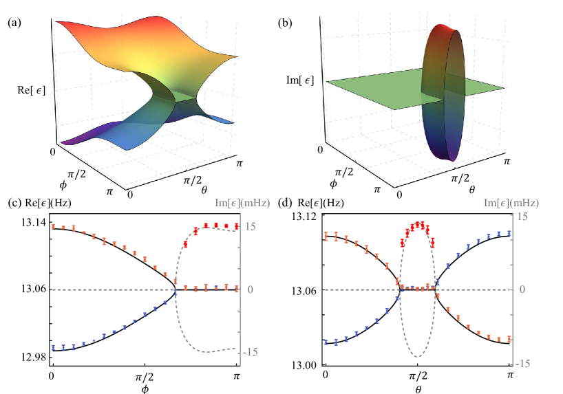
Figure 7: Non-Hermitian band structure. (a,b) The real and imaginary parts of the band structure are plotted in parametric space. The experimental results are shown through a $\theta=\pi/2$ cut in (c) and a $\phi=\pi$ cut in (d), where the orange and blue dots are real parts and the red dots represent the positive imaginary parts. The black and gray curves are the corresponding theoretical results. In experiments, we set $k=0$, $\Delta\phi=\pi$, $v_{1}/2\pi=24$ mHz, $v_{2}/2\pi=60$ mHz, $j/2\pi=30$ mHz, and $\omega_{a}/2\pi=\omega_{b}/2\pi=45$ mHz. Each data point here is acquired from five repeated measurements in two oscillators, with the error bars representing the standard error of those sets of measurements.

C.2 Edge state transition

One of the intriguing and distinct features of non-Hermitian systems is the presence of the non-Hermitian skin effect when truncating the mechanical arrays, which will lead all modes to the same edge. By varying the parameter $\theta$ on Fermi arc (moving from the edge of the Fermi arc to the center.), we find that initially, the energy tends to end up at a single edge of the system independent of which side was initially excited. That is, upon exciting at the right edge the energy remains localized there, while upon exciting at the left edge the energy propagates unidirectionally to the right and then becomes localized there. This behavior is indicative of edge localization physics being dominated by the non-Hermitian skin effect. In contrast, in the region of $\theta$ nearer to the center of Fermi arc, a portion of the initialized energy tends to stay localized at the edge. This is because the system can still host topological edge states that localize at opposite boundaries of the system, and in certain parameter regimes this symmetry consideration can dominate over the non-Hermitian skin effect.

This competition between symmetry and non-Hermitian skin effect can be understood by the analytical solution of the two surface states of our Hamiltonian in Eq. (10), satisfying

$$H\sum_{n=1}^{N}\left(a_{n}|n,A\rangle+b_{n}|n,B\rangle\right)=\epsilon_{s}\left(a_{n}|n,A\rangle+b_{n}|n,B\rangle\right).$$ (24)

This gives $2N$ equations for the amplitudes $a_{n}$ and $b_{n}$ as follows,

$$\mathrm{for~{}}n=1,2...,N-1:\quad v_{2}\text{cos}\theta~{}a_{n}+(\omega_{0}+\omega_{b}\text{cos}\phi_{b})~{}b_{n}+j~{}a_{n+1} =\epsilon_{s}~{}b_{n};$$ (25)

$$j~{}b_{n}+(\omega_{0}+\omega_{a}\text{cos}\phi_{a})~{}a_{n+1}+v_{1}\text{cos}\theta~{}b_{n+1} =\epsilon_{s}~{}a_{n+1};$$

$$\text{for boundaries}:\quad\quad\quad\quad(\omega_{0}+\omega_{a}\text{cos}\phi_{a})~{}a_{1}+v_{1}\text{cos}\theta~{}b_{1} =\epsilon_{s}~{}a_{1};$$

$$v_{2}\text{cos}\theta~{}a_{N}+(\omega_{0}+\omega_{b}\text{cos}\phi_{b})~{}b_{N} =\epsilon_{s}~{}b_{N}.$$

For the sake of computational convenience, we can decompose the on-site terms $\omega_{a}\text{cos}\phi_{a}$ and $\omega_{b}\text{cos}\phi_{b}$ into a common central frequency and a detuning frequency. This decomposition takes the form: $\omega_{a}\text{cos}\phi_{a}=\omega_{c}+\delta\omega$, $\omega_{b}\text{cos}\phi_{a}=\omega_{c}-\delta\omega$, where $\omega_{c}=\left(2\omega_{0}+\omega_{a}\text{cos}\phi_{a}+\omega_{b}\text{cos}\phi_{b}\right)/2$ and $\delta\omega=\left(\omega_{a}\text{cos}\phi_{a}-\omega_{b}\text{cos}\phi_{b}\right)/2$. The common part acts as a frequency shift, which does not influence the mode profiles. Without loss of generality, we can remove it by switching to a frame rotation at frequency $\omega_{c}$. Thus, the Eq. (25) can be rewritten in:

$$\mathrm{for~{}}n=1,2...,N-1:\quad v_{2}\text{cos}\theta~{}a_{n}-\delta\omega~{}b_{n}+j~{}a_{n+1} =\epsilon_{s}~{}b_{n};$$ (26)

$$j~{}b_{n}+\delta\omega~{}a_{n+1}+v_{1}\text{cos}\theta~{}b_{n+1} =\epsilon_{s}~{}a_{n+1};$$

$$\text{for boundaries}:\quad\quad\quad\quad\delta\omega~{}a_{1}+v_{1}\text{cos}\theta~{}b_{1} =\epsilon_{s}~{}a_{1};$$

$$v_{2}\text{cos}\theta~{}a_{N}-\delta\omega~{}b_{N} =\epsilon_{s}~{}b_{N}.$$

where the surface states satisfy $\epsilon_{s}=\pm\delta\omega$. When $\delta\omega=0$, we have two zero energy surface states. The solution to the above equation is

$$a_{n} = a_{1}\left(\frac{-v_{2}\text{cos}\theta}{j}\right)^{n-1},\quad{\rm for\ }n=1,\ldots,N;\quad\quad$$

$$b_{n} = b_{N}\left(\frac{-v_{1}\text{cos}\theta}{j}\right)^{N-n},\quad{\rm for\ }n=1,\ldots,N.$$ (27)

where $a_{N}={\sqrt{v_{2}^{2}\text{cos}^{2}\theta-j^{2}}}/{j}$ and $b_{1}={\sqrt{j^{2}-v_{1}^{2}\text{cos}^{2}\theta}}/{j}$ are normalized parameters. In the thermodynamic limit ($N\rightarrow\infty$), to satisfy the boundary condition $a_{N}=b_{1}=0$, the intercell hopping must be stronger than the intracell hopping, i.e., $v_{1(2)}\text{cos}\theta<j$. If $v_{1}\text{cos}\theta<j$ and $v_{2}\text{cos}\theta<j$, we have two zero-energy solutions, which localize at the different boundaries:

$$|L\rangle=\sum_{n=1}^{N}a_{n}|n,A\rangle,\quad|R\rangle=\sum_{n=1}^{N}b_{n}|n,B\rangle.$$ (28)

In this region, dominated by band topology, the edge states separately distribute at two ends.

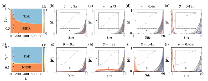
Figure 8: The edge state transition in finite-size systems. (a)  Numerically calculated TDR-NHDR diagram of edge state transition as a function of system size $L$ and $\theta$ when $\delta\omega=0$. TDR (blue region) and NHDR (orange region) are characterized by $\rm{LD}=0$, and 1, respectively. The dashed line with stars denotes four examples illustrated in (b)-(e), where the mode profiles for two surface modes (blue and orange) and bulk modes (gray) are presented with $L=60$. The insets show the corresponding energy spectra of the systems, with surface modes highlighted in blue and orange color. Here we take $v_{2}=2j=2.5v_{1}$, $\omega_{a}=2\omega_{b}=1.5j$, $\phi=\pi/2$, and $\Delta\phi=\pi$, (f)-(j) Similar studies are plotted at $\delta\omega\neq 0$, revealing the slight impact of system size on the TDR-NHDR diagram and the emergence of delocalized surface modes at transition points (h). Here we take $\phi=0.48\pi$, $\Delta\phi=\pi$, and other parameters are the same as those presented in (a)-(e).

In contrast, if $|v_{1}\text{cos}\theta|<|j|$ and $|v_{2}\text{cos}\theta|>|j|$ (assuming $|v_{2}|>|v_{1}|$), the boundary condition $a_{N}=0$ requires $a_{n}=0$ for all $n$, thus the edge states will only takes this form:

$$\quad|R\rangle=\sum_{n=1}^{N}b_{n}|n,B\rangle.$$ (29)

This result indicates the two edge states will localize at the same edge, which can be understood as driven by the non-Hermitian skin effect. The interplay and competition between band topology and non-Hermiticity leads to a transition from non-Hermitian dominance to symmetry dominance in the behavior of the localized boundary modes. The transition point where the edge states distribute at different ends to the same end is determined by the condition:

$$\rm{max}\{|v_{1}\text{cos}\theta|,|v_{2}\text{cos}\theta|\}=|j|.$$ (30)

This result is obtained under thermodynamic limit. However, in finite-sized systems, the condition will change. To quantify topological dominant region (TDR) and the non-Hermitian skin effect dominant region (NHDR), we use a mode density over the left-half cells, as defined in [49]:

$$\mathrm{LD}=\sum_{n=1}^{\lfloor N/2\rfloor}\sum_{i=\mathrm{A},\mathrm{B}}\left[\left|\phi_{n,i}^{a}\right|^{2}+\left|\phi_{n,i}^{b}\right|^{2}\right],$$ (31)

where $\lfloor N/2\rfloor$ denotes the floor function rounding down $N/2$ to its next lowest integer. The superscripts $a$ and $b$ refer to the two edge modes. The quantity LD serves as a count for the number of localized states at the left chain end. Specifically, a value of $\mathrm{LD}=1$ indicates that the two states are independently localized at the two chain ends, signifying the occurrence of TDR. On the other hand, an LD value of $0$ implies that the two states are localized at the right chain end, representing the presence of edge modes associated with NHDR.

As shown in Fig. 8(a), we plot the LD as a function of system size $L$ and coupling parameter $\theta$ to show the TDR- and NHDR-edge transition. We find that the topological dominant region becomes reduced with decreasing the system size. This is because the edge states in the thermodynamic limit are separately located at the two ends without any overlap or coupling. However, in systems with finite cells, mode coupling between the edge states becomes significant, enhancing the NHSE and expanding the non-Hermitian dominant region [49]. Besides, the delocalization behavior of the zero-edge modes under the thermodynamic limit does not occur at the transition point in finite-size systems. As shown in Fig. 8(b)-(e), the localization of the edge state undergoes a sudden transition from the same end to the opposite ends in a finite-size system with $L=60$. In contrast, when $\delta\omega\neq 0$, as depicted in Fig. 8(f), the transition points in finite-size systems align well with the point at the thermodynamic limit ($\theta=\pi/3$), revealing the slight impact of system size on the edge state transition. And at the transition point, we can observe a delocalized mode in a finite-size system ($L=60$) as shown in Fig. 8(h). This in-gap extended mode is a result of the interplay between the non-Hermitian skin effect and band topology, which reveals a promising method for wave control. As discussed in Ref. [40], they can create more specific wave patterns by the judicious engineering of the non-Hermiticity distribution. Our findings not only broaden and deepen the current understanding of the non-Hermitian edge state transition but also open new grounds for topological engineering.