PoFEL: Energy-efficient Consensus for Blockchain-based Hierarchical Federated Learning

Abstract

Facilitated by mobile edge computing, client-edge-cloud hierarchical federated learning (HFL) enables communication-efficient model training in a widespread area but also incurs additional security and privacy challenges from intermediate model aggregations and remains the single point of failure issue. To tackle these challenges, we propose a blockchain-based HFL (BHFL) system that operates a permissioned blockchain among edge servers for model aggregation without the need for a centralized cloud server. The employment of blockchain, however, introduces additional overhead. To enable a compact and efficient workflow, we design a novel lightweight consensus algorithm, named Proof of Federated Edge Learning (PoFEL), to recycle the energy consumed for local model training. Specifically, the leader node is selected by evaluating the intermediate FEL models from all edge servers instead of other energy-wasting but meaningless calculations. This design thus improves the system efficiency compared with traditional BHFL frameworks. To prevent model plagiarism and bribery voting during the consensus process, we propose Hash-based Commitment and Digital Signature (HCDS) and Bayesian Truth Serum-based Voting (BTSV) schemes. Finally, we devise an incentive mechanism to motivate continuous contributions from clients to the learning task. Experimental results demonstrate that our proposed BHFL system with the corresponding consensus protocol and incentive mechanism achieves effectiveness, low computational cost, and fairness.

1 Introduction

AS the increasing amount of data generated at end devices causes massive communication and latency overhead for traditional cloud computing, mobile edge computing (MEC) [1] has been implemented to serve end users promptly at proximity to achieve cloud computing capabilities at the edge of the network. Machine learning (ML) tasks at end devices are offloaded by sending data to edge servers for analysis and calculation. Due to data privacy and communication cost concerns, federated learning (FL) [2, 3] is introduced in MEC to form a new distributed ML paradigm, namely federated edge learning (FEL), where the edge server acts as the parameter server and proximate devices within the server’s cover range work as FL clients to train ML model collaboratively. However, since end devices are widely spread across a vast area, one single server may not be capable of implementing FEL among all of them, stimulating the idea of hierarchical federated edge learning (HFL) [4]. According to the HFL framework illustrated in Fig. 1(a), the cloud server at the top layer coordinates the training of the global model, multiple edge servers at the middle layer aggregate local models from end devices to generate intermediate models, and end devices at the bottom layer train the local models based on their local data.

(a) Traditional HFL.

(b) Blockchain-based HFL.

Figure 1: HFL frameworks.

However, the implementation of HFL still faces two major challenges: i) the single cloud server risks the whole system with the single-point failure; and ii) the layered topology introduces additional model security and privacy issues, such as model poisoning attacks by altering the intermediate models [5] and leaking the local models of end devices at the edge servers. Such inherent issues become an obstacle to deploying HFL in practice.

One promising solution is introducing the blockchain [6, 7] into HFL to omit the need for a central server, as well as provide transparent and reliable model exchanges and global model aggregations, so as to realize better security performance. As shown in Fig. 1(b), we propose a blockchain-based HFL (BHFL), where edge servers of HFL form a consortium blockchain network and exchange intermediate models on the blockchain. The global model aggregation is then performed in a distributed and traceable manner instead of the centralized way in the traditional HFL. The consortium blockchain provides a transparent and secure platform for FL, and all edge servers can track and audit the whole FL process independently. The lower layer of our proposed framework is the same as that of the traditional HFL, where each edge server and the connected clients exchange local model updates and aggregated intermediate models several times in multiple FEL iterations. Limited related work about implementing blockchain in HFL can be found in [8, 9, 10] while others involving the keywords of blockchain, hierarchical, and FL are applying hierarchical blockchain to FEL [11, 12, 13]. In [8], the authors replace the cloud server with a dedicated blockchain as the top layer, and the authors in [9, 10] append a blockchain between edge servers and the cloud server to work as a storage and record platform. Different from these existing studies deploying the blockchain as an additional part of HFL, our proposed system fully integrates blockchain with HFL through deploying blockchain on edge servers, thus being more compact and efficient compared with these existing BHFL frameworks.

Nevertheless, it is nontrivial to deploy the proposed BHFL framework. First, the existing consensus protocols cannot be arbitrarily implemented in this BHFL system since they are usually working as an additional process to determine the generator of a new block besides finishing the FL computation task, bringing extra computational overhead to edge servers and slowing down the training speed of the global model. Second, the intermediate models of edge servers need to be uploaded to the blockchain during the consensus process for verification and block generation, which makes it easy for some malicious edge servers to plagiarize models shared by other edge servers without performing the actual FEL process. Moreover, given that numerous end devices conduct FL tasks via the coordination of distributed edge servers, consuming extensive computing and communication resources, it is imperative to provide sufficient incentives to them to compensate for their cost and motivate their long-term participation.

In this paper, we design an energy-efficient consensus algorithm, named PoFEL, to address the first challenge, where the intermediate models of FEL at edge servers are utilized to determine the leader in the consortium blockchain. To solve the plagiarism issue, we design a cryptographic scheme named HCDS, combining Hash, Commitment Scheme, and Digital Signature, to validate the process of model exchanges among edge servers without worrying about their dishonesty. We employ cosine similarity to measure the difference between the aggregated global model and each intermediate model from the edge server, based on which each edge server votes the edge server with the lowest difference to be the leader node. All votes will be sent to a smart contract for vote tallying, with a weighted voting system that adopted Bayesian Truth Serum (BTS) scoring method to tackle the potential issue of bribery voting. Finally, we propose a Stackelberg game-based incentive mechanism to address the motivation challenge.

Overall, the main contributions of this work can be summarized as follow:

• We propose a BHFL framework with edge servers running the consortium blockchain for model aggregation and distributed end devices capable of collecting diverse data samples to benefit model training.

• To optimize the energy efficiency of the proposed BHFL system, we design a novel consensus algorithm, namely Proof of Federated Edge Learning (PoFEL), to reduce the extra computational cost for reaching blockchain consensus using the edge servers’ intermediate models as an evaluation metric for determining the leader node. We design a Hash-based Commitment and Digital Signature (HCDS) scheme to prevent model plagiarism in the consensus process involving model exchanges. Bayesian Truth Serum-based Voting (BTSV) is also developed to minimize the chance of bribery voting.

• To ensure the motivation of participants involved in finishing learning tasks, we proposed a two-stage Stackelberg game-based incentive mechanism to help model owners decide the rewards being distributed to each FEL cluster and facilitate the decision of edge server as the FEL coordinator regarding the optimal amount of computational resources to be spent.

• We evaluate our proposed mechanisms through extensive experiments. The experiment results prove that our mechanisms achieve low computation cost, fairness, and effectiveness.

The remainder of this paper is organized as follows. Related work is discussed in Section 2. The system workflows and adversary models are illustrated in Section 3. The consensus algorithm PoFEL is presented with details in Section 4, and an incentive mechanism based on a two-stage Stackelberg game is introduced in Section 5. Security analysis of the proposed system is given in Section 6 and experiment evaluations are presented in Section 7. Finally, we conclude the paper in Section 8.

2 Related Work

2.1 Hierarchical Federated Edge Learning

Traditional FL studies rely on a central server (e.g., cloud) to collect local models from clients. A lot of recent research has been proposed to introduce edge computing [14] into traditional FL and formulate various FEL systems [15, 4, 16, 17]. In [4], the authors propose a client-edge-cloud HFL system where edge servers are deployed as intermediate model aggregators to reduce the overall communication cost and the processing burden of the cloud, along with the design of a hierarchical FL aggregation algorithm named HierFAVG and its convergence analysis. This paper serves as a very promising and classical FEL architecture. Various following papers investigated the remaining issues of FEL systems. The authors in [15] devise a novel client-edge assignment scheme based on client location, data distribution, and communication constraints under the same FEL system architecture, where the optimization goal is to minimize FL convergence time, as well as communication and computation cost of the whole system. Similarly, Lim et al. [16] extend the FEL system proposed in [4] to support multiple model owners, where each edge server serves as a cluster head that connects with a model owner. The authors in [17] investigate the model training challenges in a Hybrid Hierarchical Federated Edge Learning (HHFEL) system with device stragglers. They design an online semi-asynchronous FL approach to improve training efficiency by optimizing resource allocation and device selection.

2.2 Blockchain-based Federated Learning

Some studies about blockchain-based federated learning (BCFL) systems directly replace the central server with a blockchain network involving a specified set of miners [18, 19, 20]. Other papers [21, 22] with alternative approaches employ FL clients as blockchain nodes without introducing additional miners. Since mining is usually computationally intensive for an FL client in addition to local model training, partial or all clients with enough computation power may work as blockchain miners for validating model updates and new block generation.

The idea of blockchain could also be applied in FEL to overcome single-point failure and other security challenges including using blockchain [23, 24, 25] or hierarchical blockchain [11, 12, 13]. Both works in [23, 24] propose similar BCFL systems for the scenario of FEL where the edge servers are responsible for aggregating local models from the local devices. The edge servers also formulate a blockchain that is responsible for consensus and auditing the local models. In [25], the authors propose a framework called FLchain, in which the blockchain is maintained by edge servers and a portion of powerful local devices. Chai et al. [12] introduce a hierarchical blockchain structure into FEL to achieve knowledge sharing among the internet of vehicles. Roadside units (RSUs) are grouped according to their locations and communication ranges, and then a ground blockchain is formulated by a group of RSUs and used for recording model updates submitted from low-level FL clients, i.e., vehicles. RSUs would integrate these model updates with their own trained model updates and then upload integrated results to the top blockchain composed of base stations. Xu et al. [13] propose a similar hierarchical blockchain-enabled FL framework in which an inter-microchain network interconnects multiple independent microchain consensus networks composed of clients and intermediate aggregators. The FL server and aggregators form the inter-microchain and a subset of them are selected as a validator committee to execute Byzantine Fault Tolerance (BFT) consensus to record microchains’ checkpoints. Both studies apply the hierarchical blockchain to FL but the extra system cost in terms of latency and energy is not discussed.

2.3 Blockchain-based Hierarchical Federated Learning

HFL proposed in [4] inspires several studies that employ blockchain in HFL. In [8], the authors propose a collaborative IoT intrusion detection system among organizations using a blockchain-based hierarchical FL framework. Given each organization possesses multiple IoT endpoints, organizations work as middle-layer servers and aggregate their collected ML-based intrusion detection models from IoT endpoints. Resulting models are further uploaded to a permissioned blockchain that works as the cloud server for global model aggregation. Zhang et al. [9] implement a data transmission model using the idea of edge computing, FL, and blockchain. Edge servers collect local model updates from low-level end devices and transmit them to the blockchain for verification and aggregation. Then the cloud server retrieves aggregated models from the blockchain and further aggregates these intermediate models into the global model. Huang et al. [10] propose a multi-layer blockchain-based HFL network consisting of an IoT devices layer, edge layer, blockchain layer, and cloud layer. After analyzing the relationships between training model error, IoT device associations, and data distribution, they propose distance-aware hierarchical federated learning (DAHFL) to minimize training model error. In all the above-mentioned studies, blockchain is deployed as an additional part of the HFL structure, without considering the extra system overhead.

Different from the existing BHFL studies [8, 9], our proposed framework is designed to be energy-efficient by empowering edge servers to form the blockchain system without employing additional miners. To tackle the challenges brought by the blockchain, we design a lightweight consensus algorithm utilizing intermediate model aggregation results for leader election, which is enhanced with plagiarism- and bribery-free schemes, and a Stackelberg game-based incentive mechanism to encourage the participation of clients.

3 System Overview

Figure 2: The topology of our proposed system.

As illustrated in Fig. 2, our proposed BHFL system has two layers: i) the upper layer is the blockchain-based federated learning (BCFL) system running on edge servers, and ii) the bottom layer includes all FEL systems with each consisting of one BCFL node and multiple end devices (i.e., clients). We refer to a BCFL node as $e_{i}$ and $E=\{e_{1},\cdots,e_{i},\cdots,e_{N}\}$ represents all BCFL nodes in the system, where $N$ is the total number of BCFL nodes.

3.1 System Workflow

Specifically, there are four main procedures in the workflow of the proposed system:

1) Task Publication: A user sends a learning task request to the BCFL network so that all BCFL nodes can receive the information and apply an evaluation scheme to determine whether they accept the task. The task information includes the user’s identity and learning task description, which will also be recorded on the blockchain.

2) Incentive Mechanism: A simple two-stage Stackelberg game-based [26] incentive mechanism is applied between the task publisher (i.e., model owner) and each participating BCFL node before beginning the following FEL procedure to determine rewards being assigned to each BCFL node and the amount of computational resource each BCFL node invests. These rewards are the payment of the FL task for an FEL cluster consisting of the BCFL node and associated end devices as compensation for training local models using their own data.

3) Federated Edge Learning: The BCFL node will distribute the learning task or updated global model to connected clients in each participating FEL cluster. Afterward, clients will prepare the training data, perform the local training and upload their model updates to their connected BCFL node. The BCFL node will aggregate received local model updates into an FEL model which will be returned to clients to begin another iteration.

4) Global Model Aggregation and Consensus in BCFL: After a specific period of FEL, the BCFL system will generate a block, containing the latest FEL models from all BCFL nodes and the resulting updated global model, and broadcast it to be recorded on the blockchain. This process is taken place at a constant rate in a round-by-round manner, and every BCFL node will participate in this process. In each round, all BCFL nodes perform the consensus mechanism to determine a leader for block generation. Each BCFL node first broadcasts its FEL model and then computes the updated global model using all received FEL models. The consensus mechanism is based on the similarity between each FEL model and the updated global model. And the BCFL node submitting the FEL model with the highest similarity will become the leader, which will be responsible for the generation of a new block storing important information, such as the leader node identity, all submitted FEL models, and the updated global model. Once all BCFL nodes have received and verified the new block through broadcasting, they will add it to their own ledger to finish the blockchain updating. More details about the consensus algorithm will be provided in Section 4.

The learning task will be terminated once the loss function of the global model is minimized or the user-specified completion time is expired.

3.2 Adversary Models

In our proposed BHFL system, there exist potential adversaries impeding the implementation of the above four main procedures, especially during the consensus process. In the below, we define the assumptions, goals, and capabilities of malicious BCFL nodes as adversary models, including model plagiarism and bribery voting.

3.2.1 Model Plagiarism

In the context of consensus algorithm in BCFL, all BCFL nodes exchange their FEL models initially to facilitate model aggregation, leader election, and verification. However, due to the distributed manner of the network, achieving simultaneous model exchanges across all nodes presents a challenge. Certain nodes may receive models earlier than others, creating an opportunity for malicious nodes to engage in model plagiarism. These nodes can exploit this time discrepancy to fabricate models as their own by plagiarizing other received models, enabling them to obtain rewards without utilizing their own computing resources.

Assumption: Adversaries can include any BCFL node within the BCFL system, without any additional resource or equipment requirements. The adversaries decide to cease the FEL process to save their own computing resources.

Goals: After receiving FEL models from other benign BCFL nodes, an adversary utilizes one or more of the received models to fabricate a new FEL model and present it as its own learned FEL model. This can be done by direct copying or editing a received model or merging several received models. Subsequently, the adversary broadcasts the plagiarized model as expected. Since there is no criteria to distinguish the plagiarized model, by following this approach, the adversary can acquire rewards for the plagiarized model for free without being recognized by other benign BCFL nodes.

Capabilities: For an adversary to benefit from the plagiarized FEL model and obtain rewards, they must possess adequate network conditions to timely broadcast the plagiarized models before the model aggregation occurs. Since the adversaries can be any BCFL node, it is capable of receiving, copying or editing, and broadcasting the FEL models.

3.2.2 Bribery Voting

Within the proposed consensus algorithm, the process of determining the leader node involves vote tallying. However, in this scenario, a malicious node has the potential to incentivize other BCFL nodes to cast dishonest votes, thus disrupting the accuracy of the tallying results.

Assumption: For adversaries to successfully bribe other BCFL nodes, they must either have access to ample rewards or ensure that the act of bribery is financially beneficial (where the earned rewards exceed the cost of bribery). Additionally, the proportion of corruptible BCFL nodes is assumed to be lower than 50%.

Goals: The adversaries gain unauthorized profits by engaging in bribery with other BCFL nodes, influencing them to vote in their favor and increasing their chances of being selected as leader nodes. Furthermore, the adversaries may choose to bribe other BCFL nodes to cast dishonest votes (random votes), thereby disrupting the integrity of the voting process.

Capabilities: The adversaries possess the ability to compromise a BCFL node, resulting in its willingness to faithfully cast votes in favor of the adversaries. Furthermore, they have covert means to distribute bribery rewards to other BCFL nodes without detection.

4 PoFEL: Energy Efficient Consensus Algorithm Design

In this section, we will first discuss our proposed consensus mechanism PoFEL, followed by the detailed design of three main sub-procedures preventing adversarial attacks defined in Section 3.2.

The overall process of our proposed consensus mechanism, named Proof of Federated Edge Learning (PoFEL), is summarized in Algorithm 1. Denote $W(k)=\{w^{{1}}(k),\cdots,w^{{i}}(k),\cdots,w^{{N}}(k)\}$ as the set of FEL models, where $w^{i}(k)$ is the aggregated model of node $e_{i}$ at BCFL round $k$, and $N$ is the total number of BCFL nodes. In each round, every BCFL node $e_{i}$ runs the Hash-based Commitment and Digital Signature (HCDS) function with its FEL model $w^{i}(k)$ as input (Line 2), which will lead to the broadcast of all FEL models and the verification of all received FEL models. Then all BCFL nodes conduct Model Evaluation (ME) to derive the updated global model $gw(k)$ from $W(k)$ (Line 3). Next, each BCFL node $e_{i}$ computes cosine similarities between each FEL model $w^{i}(k)\in W(k)$ and the updated global model $gw(k)$. Based on these similarities, $e_{i}$ will cast a vote $e^{i}_{best}(k)$ for the BCFL node with the highest similarity, along with the prediction of the voting result, denoted by $P^{i}(k)$ (Line 4). Specifically, $P^{i}(k)=\{p_{1}^{i}(k),\cdots,p_{N}^{i}(k)\}$ indicates the percentage of votes each node will receive. After gathering submissions from all nodes into $E_{best}(k)=\{e^{1}_{best}(k),e^{2}_{best}(k),\cdots,e^{N}_{best}(k)\}$ and $P(k)=\{P^{1}(k),P^{2}(k),\cdots,P^{N}(k)\}$, the smart contract for vote tally will employ the Bayesian Truth Serum-based Voting (BTSV) scheme to generate a score that represents the honesty for each BCFL node. Such a scheme utilizes Bayesian Truth Serum (BTS) to evaluate how common each BCFL node is voted compared to the common predictions in $P(k)$. The cumulative historical score is then used to calculate the voting weight of each BCFL node and tally $E_{best}(k)$ based on these weights so that the leader node $e^{*}(k)$ at round $k$ can be determined (Line 5). Eventually, the leader node will package all important information into the New Block and broadcast it to the whole BCFL system (Lines 6-7).

Algorithm 1 Overall Process of PoFEL

0:  $W(k)$

1:  while round $k$ do

2:     run HCDS ($w^{i}(k)$) at every $e_{i}$

3:     $(e^{i}_{best}(k)$, $P^{i}(k)$, $gw(k))\leftarrow$ ME ($W(k)$) at every $e_{i}$

4:     each $e_{i}$ submits $e^{i}_{best}(k)$ and $P^{i}(k)$ to smart contract

5:     $e^{*}(k)\leftarrow$ BTSV $(E_{best}(k),P(k))$

6:     $New\ Block\ \leftarrow$ $e^{*}(k),W(k),gw(k)$

7:     $e^{*}(k)$ broadcasts $New\ Block$

8:  end while

Algorithm 2 HCDS

0:  $w^{i}(k)$

1:  Initialize: $r^{{i}}(k)$

2:  $d^{i}(k)=H(r^{i}(k)\ ||\ w^{i}(k))$

3:  $tag^{i}(k)=DSign(d^{i}(k),SK_{i})$

4:  broadcast $d^{i}(k)$ and $tag^{i}(k)$

5:  receive ${D(k,i)}$ and $TAG(k,i)$

6:  for $l=1$ to $N$ and $l\neq i$ do

7:     if $DVerify(tag^{l}(k),PK_{l},d^{l}(k))$ = Accepted then

8:        Continue

9:     end if

10:  end for

11:  broadcast $r^{i}(k)$, $w^{i}(k)$, and $tag^{i}(k)$

12:  receive $R(k,i)$, $W(k,i)$, and $TAG(k,i)$

13:  for $l=1$ to $N$ and $l\neq i$ do

14:     if $H(r^{l}(k)\ ||\ w^{l}(k))$ = $d^{l}(k)$ then

15:        if $DVerify(tag^{l}(k),PK_{l},H(r^{l}(k)\ ||\ w^{l}(k)))$ = Accepted then

16:           Continue

17:        end if

18:     end if

19:  end for

4.1 Hash-based Commitment and Digital Signature

In our proposed PoFEL consensus algorithm, the broadcast of FEL models among BCFL nodes can lead to the issues of model plagiarism, where a malicious node might copy another node’s submission with or without editing, or even fabricate an FEL model via merging multiple models from others and then claims the plagiarized model. To overcome this challenge, we devise a Hash-based Commitment scheme integrated with Digital Signature (HCDS) that enforces each BCFL node to strictly follow the BHFL protocol and submit their own FEL models. The detailed process is summarized in Algorithm 2 and illustrated in Fig. 3 for better understanding.

To begin with, each BCFL node $e_{i}$ initializes a fixed-length random nonce $r^{i}(k)$ at round $k$ (Line 1), which will be concatenated with the FEL model $w^{i}(k)$ into $r^{i}(k)\ ||\ w^{i}(k)$. And then this concatenation will become the input of the Hash function $H$ to derive the digest $d^{i}(k)$ (Line 2). The digest $d^{i}(k)$, together with the private key $SK_{i}$, will be further passed to the signing algorithm $DSign$ to generate the tag $tag^{i}(k)$ (Line 3). Next, each BCFL node $e_{i}$ will broadcast its digest $d^{i}(k)$ and tag $tag^{i}(k)$ (Line 4). After all BCFL nodes finish broadcasting, each BCFL node $e_{i}$ should receive digests and tags from other BCFL nodes, denoted by ${D(k,i)}=\{d^{l}(k)\mid l\neq i\}$ and ${TAG(k,i)}=\{tag^{l}(k)\mid l\neq i\}$, respectively (Line 5). Then $e_{i}$ will run the verifying algorithm $DVerify$ to check whether each tag $tag^{l}(k)$ and the associated digest $d^{l}(k)$ are valid using the public key $PK_{l}$ of the sender node $e_{l}$ (Lines 6-10). We refer to the above steps as Commit Stage.

For clarity, the workflow of this stage is presented in Fig. 3(a), where the upper half part corresponds to applying Hash function $H$ and $DSign$ successively; while the bottom half refers to $e_{i}$ utilizing $DVerify$ to validate each received digest $d^{l}(k)$ and tag $tag^{l}(k)$.

Afterwards, each BCFL node $e_{i}$ will broadcast its random nonce $r^{i}(k)$, FEL model $w^{i}(k)$ and tag $tag^{i}(k)$ (Line 11), followed by receiving random nonces, FEL models, and tags from other BCFL nodes (Line 12). The random nonces set received by $e_{i}$ is denoted as $R(k,i)=\{r^{l}(k)\mid l\neq i\}$ and the set of FEL models is $W(k,i)=\{w^{l}(k)\mid l\neq i\}$. Finally, $e_{i}$ applies the Hash function to the concatenation of received random nonce $r^{l}(k)$ and FEL model $w^{l}(k)$, and the output will be compared with the previously received digest $d^{l}(k)$. If two values match, the $DVerify$ algorithm will be utilized again to check the validity of tag $tag^{l}(k)$ and the output of the Hash function given the public key $PK_{l}$ of the sender BCFL node $e_{l}$ (Lines 13-19). We refer to these steps as Reveal Stage, and the corresponding workflow is presented in Fig. 3(b) with broadcast and reception steps omitted.

Once the HCDS scheme is accomplished, each BCFL node $e_{i}$ completes the broadcast and verifies all FEL models. It is worth noting that in addition to the common Digital Signature algorithm with the Hash function, the only extra overhead in our scheme is generating a fix-length random nonce for each FEL model, and thus it is a relatively lightweight scheme.

(a) Commit Stage

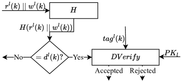
(b) Reveal Stage

Figure 3: Workflow of Commit Stage and Reveal Stage in HCDS.

4.2 Model Evaluation

Next, we design a lightweight algorithm that reuses the computational resource consumed in finishing FL tasks, namely Model Evaluation (ME), to determine the leader node in each BCFL round based on the similarities between each FEL model and the updated global model.

The details of the ME function are reported in Algorithm 3. Once the broadcast and verification of all FEL models are completed, each BCFL node $e_{i}$ will first perform the aggregation of all FEL models in $W(k)$ according to

$$gw(k)=\frac{\sum_{m=1}^{N}\left|DS_{m}\right|w^{m}(k)}{\left|DS\right|},$$ (1)

where $DS=\bigcup_{m=1}^{N}{DS}_{m}$ (Line 1), with ${DS}_{m}$ representing the combination of all clients’ local datasets associated with the BCFL node $e_{m}$, $\left|DS_{m}\right|$ is the data size of ${DS}_{m}$, and $\left|DS\right|$ refers to the total data size of $DS$.

With the help of ME, each node $e_{i}$ can calculate cosine similarity between each FEL model $w^{m}(k)$ and the updated global model $gw(k)$ to measure their difference

$$s_{m}=\frac{\left\langle w^{m}(k),gw(k)\right\rangle}{\left\|w^{m}(k)\right\|\left\|gw(k)\right\|},$$ (2)

where $\left\langle\cdot,\cdot\right\rangle$ means dot product, and $\left\|\cdot\right\|$ refers to $l_{2}$ norm.

Eventually, of all computed cosine similarities, each BCFL node $e_{i}$ will cast a vote on the BCFL node with the highest cosine similarity value at round $k$, indicating that its FEL model is the closest to $gw(k)$. We denote the index of this BCFL node as $e^{i}_{best}(k)$ (Lines 2-5).

Next, we define $p_{j}^{i}(k)\in\left[0,1\right]$ to represent node $e_{i}$’s prediction about the fraction of voters voting for node $e_{j}$ as the leader. It is clear that $\sum_{j=1}^{N}p_{j}^{i}(k)=1$. Then every $e_{i}$ can derive the prediction set $P^{i}(k)=\{p_{1}^{i}(k),p_{2}^{i}(k),\cdots,p_{N}^{i}(k)\}$ and submit it to the smart contract for tallying votes (Lines 6-13). Now, every $e_{i}$ will assign a value to $p_{j}^{i}(k)$: if $j=e_{best}^{i}(k)$, $p_{j}^{i}(k)=G_{max}$ that is close but not equal to 1 (Line 8); otherwise, $p_{j}^{i}(k)=G_{min}$ that is close to 0 (Line 10).

Algorithm 3 ME

0:  $W(k)$, $DS$

0:  $e_{best}^{i}(k)$, $P^{i}(k)$, $gw(k)$

1:  $gw(k)\leftarrow$ update via (1)

2:  for $m=1$ to $N$ do

3:     $s_{m}\leftarrow$ update via (2)

4:  end for

5:  $e_{best}^{i}(k)\leftarrow$ index of the BCFL node with highest $s_{m}$ voted by BCFL node $e_{i}$ at round $k$

6:  for $j=1$ to $N$ do

7:     if $j=e_{best}^{i}(k)$ then

8:        $p_{j}^{i}(k)\leftarrow G_{max}$

9:     else

10:        $p_{j}^{i}(k)\leftarrow G_{min}$

11:     end if

12:  end for

13:  return  $e_{best}^{i}(k)$, $P^{i}(k)$, $gw(k)$

4.3 Bayesian Truth Serum-based Voting (BTSV) for Leader

Now, we need to tally votes from all BCFL nodes and elect the leader node $e^{*}(k)$ with the highest votes. As analyzed in Section 3.2.2, however, a plain voting scheme can suffer from the threat of bribery voting, where a malicious node may corrupt or bribe some other nodes to be voted, interrupting the tallying integrity and leading to biased results. Therefore, BTSV is developed to count votes in the form of a smart contract. BTS [27] is a scoring approach that assigns higher scores to voters picking the common options. The underlying rationale is if a voter indeed has a preference for an option, s/he tends to believe others have similar preferences. As for a voter with a relatively low cumulative score, predefined penalties will be incurred, such as reward reduction or lower voting weight during tallying.

In our framework, we design BTSV that associates the cumulative score with the voting weight of each BCFL node $e_{i}$ when tallying and thus motivates BCFL nodes to vote honestly. Initially, the smart contract processes the vote $e_{best}^{i}(k)$ and vote predictions $P^{i}(k)$ from BCFL node $e_{i}$ to compute its BTS score. The BTS score reflects the behavior of the BCFL node, rewarding honest nodes with higher scores and penalizing malicious nodes with lower scores (further analysis is provided in Section 6.3). Subsequently, the system determines the voting power of each BCFL node $e_{i}$ by considering its cumulative historical BTS score. A sigmoid function is employed to transform this cumulative BTS score into a weight, ensuring the voting weight is appropriately scaled and constrained within a specific range. Specifically, when the cumulative BTS score is lower, the weight approaches 0, and as the cumulative BTS score increases, the weight also increases to approaching the maximum value. This mechanism ensures that nodes with higher cumulative BTS scores have stronger voting power, while those with lower scores have a limited influence on the voting process. Finally, the votes are tallied, and the leader node with the highest adjusted votes is selected. The detailed procedures are summarized in Algorithm 4.

Algorithm 4 BTSV

0:  $E_{best}(k)$, $P(k)$

0:  $e^{*}(k)$

1:  for $j=1$ to $N$ do

2:     for $i=1$ to $N$ do

3:        if $j$ = $e^{i}_{best}(k)$ then

4:           $A_{j}^{i}(k)\leftarrow$ 1

5:        else

6:           $A_{j}^{i}(k)\leftarrow$ 0

7:        end if

8:     end for

9:     $\overline{x}_{j}\leftarrow$ (3)

10:     $\overline{y}_{j}\leftarrow$ (4)

11:  end for

12:  for $i=1$ to $N$ do

13:     $information\ score\leftarrow$ (5)

14:     $prediction\ score\leftarrow$ (6)

15:     $score^{i}(k)\leftarrow$ (7)

16:     $CHS^{i}(k)\leftarrow$ (8)

17:     $WV^{i}(k)\leftarrow$ (9)

18:  end for

19:  for $j=1$ to $N$ do

20:     $advotes_{j}\leftarrow$ (10)

21:  end for

22:  $e^{*}(k)\leftarrow$index of the BCFL node with the highest $advotes_{j}$ at round $k$

23:  return  $e^{*}(k)$

We first define

$$A_{j}^{i}(k)=\begin{cases}1&\text{if $e_{i}$ votes for $e_{j}$ at round $k$},\\ 0&\text{otherwise}.\end{cases}$$

Then we calculate

$$\overline{x}_{j}=\frac{1}{N}\sum_{i=1}^{N}A_{j}^{i}(k),$$ (3)

and

$$\overline{y}_{j}=\exp(\frac{1}{N}\sum_{i=1}^{N}\log{p_{j}^{i}(k)}),$$ (4)

where $\overline{x}_{j}$ represents the percentage of votes that BCFL node $e_{j}$ actually receives and $\overline{y}_{j}$ means the average predicted percentage of votes that BCFL node $e_{j}$ receives (Lines 1-11). The score of the BCFL node $e_{i}$ for a vote for $e_{j}$ is defined by $\log{\frac{\overline{x}_{j}}{\overline{y}_{j}}}$. Thus, the information score for the BCFL node $e_{i}$ is calculated as follows

$$information\ score=\sum_{j=1}^{N}A_{j}^{i}(k)\log{\frac{\overline{x}_{j}}{\overline{y}_{j}}},$$ (5)

and the prediction score is denoted by

$$prediction\ score=\alpha\sum_{j=1}^{N}\overline{x}_{j}\log{\frac{p_{j}^{i}(k)}{\overline{x}_{j}}}.$$ (6)

The total score of $e_{i}$ at round $k$, denoted as $score^{i}(k)$, is calculated as follows

$$score^{i}(k) =information\ score+prediction\ score,$$

$$=\sum_{j=1}^{N}A_{j}^{i}(k)\log{\frac{\overline{x}_{j}}{\overline{y}_{j}}}+\alpha\sum_{j=1}^{N}\overline{x}_{j}\log{\frac{p_{j}^{i}(k)}{\overline{x}_{j}}}.$$ (7)

We let $\alpha=1$ so that this vote tallying process can be regarded as a zero-sum game. After deriving $score^{i}(k)$ for $e_{i}$, the cumulative historical score (CHS) of $e_{i}$ at round $k$, denoted as $CHS^{i}(k)$, is computed by

$$CHS^{i}(k)=\sum_{max(0,k-c)}^{k}score^{i}(k),$$ (8)

where $c$ is configurable and refers to the number of past rounds considered in determining CHS. Then a sigmoid function is applied to derive the weight of the vote (WV) that $e_{i}$ casts at round $k$, denoted as $WV^{i}(k)$, as follows,

$$WV^{i}(k)=\frac{\beta}{1+e^{-\theta CHS^{i}(k)-\epsilon}},$$ (9)

where $\beta$, $\theta$, and $\epsilon$ are positive coefficients (Lines 12-18). Specifically, $\beta$ determines the upper limit of WV, $\theta$ decides the gradient of WV against CHS (i.e., how quickly WV decreases when CHS drops), and $\epsilon$ assigns the value of WV as 1 when CHS is 0 since it implies that the node has never been rewarded or penalized before. A sigmoid function is chosen as it limits the range of WV with an ”S” shape, where too-small or too-large CHS results in a smoother change of WV. This aligns with our objective of strongly rewarding or penalizing nodes when they start showing good or bad behaviors instead of reaching extreme cases. Based on $WV^{i}(k)$ assigned to each BCFL node voter $e_{i}$, adjusted tallied votes $advotes_{j}$ that BCFL node $e_{j}$ receives are computed by (Lines 19-21)

$$advotes_{j}=\sum_{i=1}^{N}WV^{i}(k)A_{j}^{i}(k).$$ (10)

Eventually, the leader node with the highest adjusted tallied votes $advotes_{j}$ at round $k$ will be selected. We denoted the index of this leader node as $e^{*}(k)$ (Line 22).

5 Incentive Mechanism

To motivate end devices to contribute to FEL tasks continuously and encourage BCFL nodes to maintain the blockchain, block generation rewards to BCFL nodes and FEL rewards to the FEL clusters are required. The leader node selected by the consensus algorithm at each BCFL round will acquire a fixed number of rewards. These rewards come from the task publisher’s budget and could be determined when the learning task is initially published. Thus, in this section, we mainly focus on designing an incentive scheme to distribute FEL rewards through BCFL nodes from the FL task publisher to the clients contributing to the learning task.

The task publisher will provide rewards to motivate FEL clusters to work on the requested learning task. Rewards for an FEL cluster are first determined between the task publisher and the BCFL node, who will distribute rewards to end devices according to a pre-defined rule. An example distribution rule could be based on the CPU cycle frequency spent by each end device. In our framework, the major challenge of incentive mechanism exists at the blockchain level between the task publisher and BCFL nodes.

To that aim, we model a two-stage Stackelberg game between the task publisher and each participating BCFL node before running FEL, which can be described as below:

• Stage 1: The task publisher will set the total rewards $\delta$ for all engaging BCFL nodes by maximizing its own utility. This utility function is based on its expectation, expenditure (rewards $\delta$), and total CPU cycle frequencies consumed by all engaging BCFL nodes.

• Stage 2: After calculating received individual rewards, each BCFL node $e_{i}$ will the total CPU cycle frequency $f_{i}$ spent by its connected devices by optimizing its individual utility.

Backward induction is adopted to solve the two-stage Stackelberg game. In other words, we will start with optimizing the strategy of Stage 2 first and then analyze the best strategy of Stage 1.

5.1 Utility Function

The task publisher’s expectation of the total rewards $\delta$ paid to all engaging BCFL nodes is closely related to the total CPU cycle frequencies consumed by all FEL clusters, denoted by $F=\sum_{i=1}^{N}f_{i}$. In other words, given the total CPU cycle frequencies $F$, the task publisher can derive the optimal total rewards, denoted by $\delta^{*}$, that it believes to be the best total price paid to all participating BCFL nodes. Any rewards different from the optimal will lead to a decrease in the task publisher’s utility. This relationship could be captured by a parabola that opens downwards. Thus, the utility of the task publisher is defined as

$$U_{tp}(\delta)=B-(\lambda\frac{\delta}{F}-\varphi)^{2},$$ (11)

where $B$, $\lambda$, and $\varphi$ are coefficients reflecting the task publisher’s expectation of total rewards $\delta$ given $F$. Mathematically speaking, they determine the shape, location, and opening direction of the parabola in the plane. The utility model defined in (11) needs to satisfy $U_{tp}(\delta)>0$ and $\frac{\varphi}{\lambda}>0$. By solving the first constraint, we have $-\sqrt{B}<\lambda\frac{\delta}{F}-\varphi<\sqrt{B}$. These inequations refer to the model owner’s utility being positive when optimal rewards are given.

We assume that the total CPU cycles used for training data samples in the learning task are $\mu_{i}$. Then the energy cost of computing the task could be defined as $\gamma_{i}\mu_{i}f_{i}^{2}$ based on the popular energy consumption model [28]. Parameter $\gamma_{i}$ is related to the CPU’s architecture.

Therefore, we can derive the utility of BCFL node $e_{i}$ as

$$U_{i}(f_{i})=\delta\frac{f_{i}}{f_{i}+\sum f_{-i}}-\gamma_{i}\mu_{i}f_{i}^{2},$$ (12)

where $\sum f_{-i}$ refers to the summation of CPU cycle frequencies of all BCFL nodes except for the CPU cycle frequency $f_{i}$ of the BCFL node $e_{i}$ and can be considered as a constant.

5.2 Equilibrium Analysis

In this subsection, we will acquire the Nash equilibrium from deriving the optimal strategies for both the task publisher and BCFL nodes.

Definition 5.1.

(Stackelberg Equilibrium Strategy). The Stackelberg equilibrium strategies ($\delta^{*}$, $f_{i}^{*}$) formulate the best response of each player in the Stackelberg game, where $\delta^{*}=\arg\max_{\delta>0}U_{tp}(\delta)$ and $f_{i}^{*}=\arg\max_{f_{i}>0}U_{i}(f_{i})$.

The second stage of the game is a non-cooperative game. For any total rewards $\delta$ given by the task publisher and other BCFL node’s strategies, BCFL node $e_{i}$ will decide an optimal strategy $f_{i}^{*}$ to maximize its individual utility.

Definition 5.2.

(Nash Equilibrium). A set of strategies $f^{*}=(f_{1}^{*},\cdots,{f_{N}}^{*})$ is a Nash equilibrium of the second stage if for each BCFL node $e_{i}$ and any $f_{i}$, there exists $U_{i}(f_{i}^{*})\geq U_{i}(f_{i})$.

Theorem 5.1.

The optimal strategy $f_{i}^{*}$ of BCFL node $e_{i}$ is derived by letting the first order derivative equal 0.

Proof.

To study the Nash equilibrium of the second stage of the game, the first-order derivative of $U_{i}(f_{i})$ with respect to $f_{i}$ is derived as

$$\partialderivative{U_{i}(f_{i})}{f_{i}}=\frac{\delta}{\sum f_{-i}+f_{i}}-2f_{i}\mu_{i}\gamma_{i}-\frac{\delta f_{i}}{(\sum f_{-i}+f_{i})^{2}}.$$

The second-order derivative of $U_{i}(f_{i})$ with respect to $f_{i}$ is derived as

$$\partialderivative[2]{U_{i}(f_{i})}{f_{i}}=\frac{2\delta}{(\sum f_{-i}+f_{i})^{2}}(\frac{f_{i}}{\sum f_{-i}+f_{i}}-1)-2\mu_{i}\gamma_{i},$$

which is negative since $\frac{f_{i}}{\sum f_{-i}+f_{i}}$ is always less than 1. Therefore, the utility of BCFL node $e_{i}$ defined in (12) is a strictly concave function for $f_{i}>0$. And there exists $f_{i}^{*}$ that maximizes $U_{i}$, which can be derived via solving $\partialderivative{U_{i}(f_{i})}{f_{i}}=0$.

∎

Then the optimal value of total CPU cycle frequencies $F$ can be calculated by

$$F^{*}=\sum_{i=1}^{N}f_{i}^{*}.$$ (13)

Given the above analysis, the task publisher knows that there exists a unique Nash equilibrium among BCFL nodes given any total rewards $\delta$. Therefore, the task publisher will maximize its utility by choosing the optimal total rewards $\delta^{*}$.

Theorem 5.2.

The optimal strategy of the task publisher is given

$$\delta^{*}=\frac{{F^{*}}\varphi}{\lambda}.$$ (14)

Proof.

The first-order derivative of $U_{tp}(\delta)$ with respect to $\delta$ is derived as

$$\partialderivative{U_{tp}(\delta)}{\delta}=\frac{2\lambda(F^{*}\varphi-\delta\lambda)}{{F^{*}}^{2}}.$$

Then the second-order derivative of $U_{tp}(\delta)$ with respect to $\delta$ is derived as

$$\partialderivative[2]{U_{tp}(\delta)}{\delta}=-\frac{2\lambda^{2}}{F^{2}},$$

which is clearly negative. Therefore, the utility of task publisher defined in (11) is a strictly concave function for $\delta>0$. That is, there exists a $\delta^{*}$ maximizing $U_{tp}$.

By letting $\partialderivative{U_{tp}(\delta)}{\delta}=0$, we have

$$\delta^{*}=\frac{{F^{*}}\varphi}{\lambda}.$$

∎

6 Security Analysis

6.1 Model Plagiarism

In BCFL, the consensus algorithm usually requires all BCFL nodes to exchange their models in the first step for model aggregation, leader election, and verification. However, in this sort of distributed network, it is difficult to achieve model exchanges at all nodes at the same time. In other words, some nodes could receive models much earlier than others. This provides a chance for malicious nodes that received models earlier to plagiarize models so that they could obtain rewards without consuming their own resources. To solve this problem, we design HCDS scheme to make the model plagiarism impossible, or not worthy compared to behaving legally, where the employed Hash-based Commitment computationally hides any model $w$. Furthermore, even if the adversary can find $r\ ||\ w$ from $H(r\ ||\ w)$ given enormous computation power, the exact value of $w$ still cannot be derived. This means it is practically impossible to plagiarize any models from others after the Commit Stage in Algorithm 2.

Regarding the binding constraint, even if a malicious node tries to broadcast $r^{\prime}\ ||\ w^{\prime}$ at Reveal Stage instead of the original committed $r\ ||\ w$ at Commit Stage, the chance that revealed $r^{\prime}\ ||\ w^{\prime}$ equals to committed $r\ ||\ w$ and $w^{\prime}$ coincidentally matches a model weight committed earlier by another BCFL node is extremely low. If the malicious node finds it challenging to obtain a valid copy $w^{\prime}$ from another BCFL node such that $r^{\prime}\ ||\ w^{\prime}$ equals to $r\ ||\ w$, and it is computationally infeasible to infer $w$ from $H(r\ ||\ w)$, the BCFL node will be demotivated to plagiarize.

6.2 DDoS

Since the leader is determined by the consensus algorithm based on the model similarity evaluation and trustworthy voting, it is impossible to know in advance about the leader node that is highly possible to change every round. In this case, a constantly effective DDoS attack against the leader node cannot be achieved.

6.3 Bribery Voting

In the proposed consensus algorithm, vote tallying is involved in deriving the leader node. In this case, a malicious node could bribe other BCFL nodes to cast dishonest votes to interfere with tallying results. Thus, we introduce the BTS into the weighted voting process to encourage BCFL nodes to behave honestly. Given that BCFL node $e_{i}$ votes for an option, its information score would be lower if the actual fraction of votes received by this option is lower than the average predicted fraction of votes that this option receives. And the prediction score gives a penalty if the BCFL node $e_{i}$’s predicted fraction of votes that an option receives is lower than the actual fraction of votes. The more commonly this option is voted, the more penalty is given.

Both malicious and honest nodes will cast a vote for an option, and assign a predicted fraction of votes this option receives to $G_{max}$ while other options as $G_{min}$. This means that for every option, the actual fraction of votes it receives is always roughly the same as the average predicted fraction of votes it receives. The information scores for both malicious and honest nodes are not distinguishable. But malicious nodes that cast votes for a BCFL node other than the correct one with the highest $s_{m}$ will be penalized by prediction score as it receives a huge penalty for low prediction on the votes the correct BCFL node should receive (as the correct BCFL node receives a higher fraction of votes). Thus, the overall score of malicious nodes will be lower than that of honest nodes. Then the system will impose lower weights on the votes cast by malicious nodes since their CHS tend to be lower. Lower weights on the votes reduce the voting power of the malicious nodes and weaken their impacts on the vote tallying process.

7 Experimental Evaluation

In this section, we perform several experiments to verify the effectiveness and efficiency of our proposed consensus algorithm and incentive mechanism. All experiments are conducted using Google Colab with Python 3.6.9 running on single core hyper threaded Intel(R) Xeon(R) CPU at 2.3GHz, Tesla T4 GPU, and 13GB memory.

7.1 Experiment Setups and Dataset

We implement the BHFL system where each FEL cluster involves five local clients. Each BCFL node will perform FEL with its associated clients three times before exchanging FEL models with other BCFL nodes at the BCFL system. The default number of BCFL nodes involved is set to 50.

1) Dataset: The FL task is conducted on MNIST [29] dataset using the MLP model. The MNIST dataset is a collection of handwritten digits that is widely used as a benchmark for image recognition algorithms. It consists of 60,000 training images and 10,000 testing images, with each image being a grayscale 28x28 pixel image of a handwritten digit from 0 to 9. All training images are used to train the model and randomly distributed to every end device.

2) Model: We utilize a multilayer perception (MLP) model which consists of a flatten layer, a hidden layer with ReLU activation, a dropout layer with a frequency of 0.2, and an output layer with softmax activation. The flatten layer is used to map the original image data to a one-dimensional array that contains 784 elements (28*28) which can be read by the hidden layer. The hidden layer is made up of 128 neurons by default. The output layer contains 10 neurons that correspond to the 10 labels in the MINST dataset. The stochastic gradient descent (SGD) optimizer is used with a learning rate of 0.001, a decay factor equal to half of the learning rate, and a momentum value of 0.9.

7.2 Evaluation of HCDS

HCDS consists of two stages: Commit Stage and Reveal Stage, and we evaluate them separately. The Hash function and Digital Signature Algorithm used in the experiment are SHA-256 and Elliptic Curve Digital Signature Algorithm (ECDSA) [30], respectively. The results reported are derived by averaging results for ten rounds of repeated experiments.

We first investigate the computation cost in Commit Stage, which involves three computational functions: Hash function $H$, $DSign$, and $DVerify$. We first study the impacts of MLP model complexity and random nonce length on Hash function $H$ and $DSign$. As shown in Lines 2-3 in Algorithm 2, the only factors that will affect the time cost of $H$ and $DSign$ are inputs $r^{i}(k)$ and $w^{i}(k)$, which are specifically the random nonce length and the MLP model complexity. To model changes in the complexity of the MLP model, we change the number of neurons in the hidden layer in the MLP model. As shown in Fig. 4(a), the time cost increases linearly with the length of the random nonce length. Furthermore, the rise in the amount of time cost caused by the change in model complexity is almost constant regardless of the random nonce length given. All these trends are consistent with the inherent attributes of the selected Hash function $H$ and Digital Signature Algorithm.

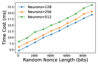
(a) Model Complexity and Random Nonce Length vs. $H$ and $DSign$ cost.

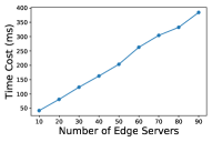
(b) Network Size vs. $DVerify$ cost.

Figure 4: Computation Cost in Commit Stage.

Then we examine the impact of BCFL network size $N$ on the computation cost of $DVerify$. The result is illustrated in Fig. 4(b). More BCFL nodes in the network bring more FEL models for $DVerify$ to execute at BCFL node $e_{i}$. Similarly, a linear relationship between the time cost and the number of BCFL nodes is observed, and such a relationship matches with the Digital Signature Algorithm used.

Finally, we analyze the impact of BCFL network size, random nonce length, and model complexity on the computation cost in Reveal Stage, which involves the Hash value computations and $DVerify$. Thus all previously mentioned factors will impact the computation cost in Reveal Stage. Fig. 5(a) demonstrates a linear trend between the number of BCFL nodes and time cost. We also notice that the impact of the random nonce is inconspicuous on the relationship between the number of BCFL nodes and time cost. We could infer the reason by comparing Fig. 4(b) and Fig. 5(a). The random nonce length will affect the time taken by Hash function $H$ but not $DVerify$. And the inputs of $DVerify$ are tags and digests, which are all fixed given the same Hash function $H$ and $DSign$. This could imply that the amount of time increased in Hash function $H$ due to the change of the random nonce length is minor compared with the total amount of time needed by $DVerify$ and Hash function $H$.

On the other hand, the model complexity gradually impacts the trend between the time cost and the number of BCFL nodes, as shown in Fig. 5(b). The more significant number of neurons leads to more time cost computing the Hash value for a single FEL model, and more BCFL nodes mean more FEL models to process. Therefore, a steeper trend between the time cost and the number of BCFL nodes is observed when the number of neurons is more considerable (more accumulated additional time cost of a single FEL model).

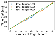
(a) Random Nonce Length & Network Size.

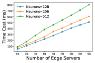
(b) Model Complexity & Network Size.

Figure 5: Computation Cost in Reveal Stage.

7.3 Experiments on Model Evaluation

In this subsection, experiments are designed to analyze the computation cost and the randomness of the ME mechanism. Randomness refers to the difference in the chance of each BCFL node participating in the same FL task being selected as the leader. The randomness metric directly reflects the fairness of ME. The input of the ME scheme is FEL models. Therefore, the number of BCFL nodes and the model complexity will affect its computation time.

First, we will investigate the impact of the number of BCFL nodes and the model complexity on the time cost of the ME mechanism. Experimental results are plotted in Fig. 6(a). The number of BCFL nodes and the time cost of ME demonstrates a linear trend. We can see that when the number of neurons is small, the trend between the number of BCFL nodes and the time cost is mild. This indicates the same reason as explained in Fig. 5(b) that more neurons cause more time for ME to compute the similarity of one FEL model. Thus, more BCFL nodes (more FEL models to proceed) lead to increased accumulated time costs.

Then we evaluate the randomness of our proposed ME scheme. We implement two distribution types of the clients’ data: independent and identically distributed (IID) and non-IID. For non-IID, each client possesses data with roughly six out of ten labels in the MNIST dataset. For IID, data with all labels are available to each client. Fig. 6(b) presents the number of times each BCFL node is selected as the leader before the global model of the FL task is converged. Observations indicate less fairness when the data distribution is non-IID. This could be caused by the dominance of several BCFL nodes having more labels available on their associated clients’ local data compared with other BCFL nodes. Given more diverse data, the FEL model learned is more representative. The chance of the BCFL node being selected as the leader increases. The randomness of ME is closely related to the actual distribution of the data possessed by each client.

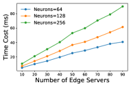
(a) Model Complexity and Network Size.

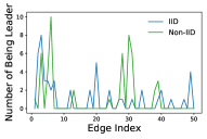
(b) Different Clients’ Data Distribution.

Figure 6: Computation Cost and Randomness of ME.

7.4 Evaluation of Bayesian Truth Serum-based Voting

We validate the effectiveness of the BTSV by demonstrating its ability to distinguish malicious BCFL nodes from honest ones and limit their influences on voting results through the differences in the weight of votes (WV). Here we refer to honest and malicious BCFL nodes as honest nodes (HNs) and malicious nodes (MNs), respectively. For comparison, we design two attack strategies: targeted attack (TA) and random attack (RA), where TA means that all MNs collude with each other and vote the same BCFL node as the leader, while RA implies that each MN randomly casts a vote for a BCFL node. Also, the value of $G_{max}$ is set to 0.99 and $G_{min}$ is $\frac{1-0.99}{N-1}$ for model evaluation. We denote the chance of a malicious node behaving maliciously as CBM. And CHS considers 20 consecutive rounds of historical scores if available (i.e., $c$ is set to 20). Coefficients $\beta$, $\theta$, and $\epsilon$ used to derive WV are set to 1.3, 0.4, and 1.2, respectively. As discussed in Section 4.3, these coefficients limit the range of $WV^{i}(k)$ between 0 and 1.3, and ensure $WV^{i}(k)\approx 1$ when CHS is 0. Other coefficients derive similar results as the changing trend mainly depends on CHSs.

By comparing the BTSV under these two attack strategies, we present the experimental results in Fig. 7. The differences in the average weight of the vote of HNs and MNs are clear after several rounds of BTSV iterations. It can be seen that all the trends of voting weight under RA are steeper than that under TA. This means the difference between voting weights is more obvious under RA, while TA is always more difficult to be restricted than RA regardless of the proportion of MNs and the probability of MNs performing attacks.

We first discuss how the probability of MNs performing attacks (CBM) affects the difference in voting weights between HNs and MNs under both attack strategies. By comparing Figs. 7(a) and 7(b) or Figs. 7(c) and 7(d), with the same proportion of MNs, more difference in voting weights is observed when CBM increases under both attacks. Thus it is easier to have the attack recognized and penalized when the probability of MNs performing attacks is high.

Then we investigate how the proportion of MNs impacts the difference in voting weights between HNs and MNs. By comparing Figs. 7(a) and 7(c) or Figs. 7(b) and 7(d), with the same CBM, less difference in voting weights is observed when the proportion of MNs raises under TA, while the difference under RA remains similar. This indicates that changes in the proportion of MNs do not affect the amount of penalty imposed on MNs under RA. While for TA, when either the proportion of MNs is low or CBM is high, more penalties on voting weights will be distributed to MNs.

Lastly, we analyze the corresponding reasons from the perspective of BTS score. This score represents how common the selected option is compared to the common prediction, and the prediction score measures the difference between the actual and predicted distribution of selections. In RA, a rise in the proportion of MNs will lead to the same increase in score components for MNs and HNs because additional MNs vote for random BCFL nodes instead of already cast votes. This introduces the same additional elements for summation in (3), (4), and (6), thus leading to the same increase in eventual scores and consequently a similar difference between average WV for both MNs and HNs. However, this is not the case for TA since a change in the probability of MNs performing attacks or the proportion of MNs will cause a direct value difference in the information and prediction score components (the number of votes for the same selection is changed). Such differences are amplified after deriving the weight of the vote using a sigmoid function.

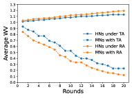
(a) 20% MNs, CBM=30%.

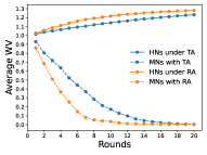
(b) 20% MNs, CBM=70%.

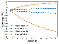
(c) 40% MNs, CBM=30%.

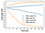
(d) 40% MNs, CBM=70%.

Figure 7: Average weight of the vote for Honest Nodes (HNs) and Malicious Nodes (MNs) Performing Targeted Attack (TA) vs. Random Attack (RA).

7.5 Evaluation of Incentive Mechanism

Finally, we study the effects of strategies of the task publisher $\delta$ and BCFL nodes $f_{i}$ on utility functions. In this experiment, we set $B$ = 500, $\varphi$ = 5, $\lambda$ = 1, $\mu_{i}$ = 5, $\sum f_{-i}=1000$ and $\gamma_{i}$ = 0.01 to satisfy constraints of utility functions.

First, impacts of the total rewards $\delta$ and total CPU cycle frequencies $F$ on the model owner’s utility are evaluated. The total CPU cycle frequencies $F$ is set to 1000 when evaluating the strategy of model owner $\delta$. And the total rewards $\delta$ is set to 5000 when evaluating the sum of strategies of BCFL nodes $F$. As illustrated in Fig. 8(a), the model owner’s utility $U_{tp}$ is inversely proportional to $F$. This is as expected as the denominator of $U_{tp}$ is $F$. Fig. 8(c) demonstrates the existence of the optimal strategy $\delta$ for the model owner.

Next, we evaluate the impacts of the total rewards $\delta$ and total CPU cycle frequency $f_{i}$ on a BCFL node $e_{i}$’s utility. The total CPU cycle frequency $f_{i}$ is set to 40 when evaluating the strategy of model owner $\delta$. The total rewards $\delta$ is set to 5000 when evaluating the strategy of BCFL node $e_{i}$. It can be seen in (12), the BCFL node $e_{i}$’s utility $U_{i}$ and $\delta$ show a linear relationship, as indicated in Fig. 8(b). Similarly, Fig. 8(d) demonstrates the existence of the optimal strategy $f_{i}$ for BCFL node $e_{i}$.

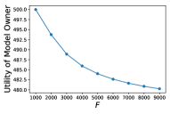
(a) $F$ vs. $U_{tp}$.

(b) $\delta$ vs. $U_{i}$.

(c) $\delta$ vs. $U_{tp}$.

(d) $f_{i}$ vs. $U_{i}$.

Figure 8: Impact of $F$ and $\delta$ on Utility Functions $U_{tp}$ and $U_{i}$.

8 Conclusion

In this paper, we propose a BHFL framework with a novel efficient consensus algorithm to avoid extra waste of computation resources during blockchain consensus. The consensus algorithm utilizes intermediate models from BCFL nodes and compares each model with the updated global model for leader node election. Additionally, we combine the Hash-based Commitment and Digital Signature Algorithm to resolve the model plagiarism issue that occurs during the model exchange process; and we also employ BTSV in the vote tally smart contract for determining the leader node so as to prevent voting bribery from malicious nodes. A two-stage Stackelberg game is modeled to design the incentive mechanism, providing motivation for clients in the FEL clusters to contribute to the learning task. Experimental results demonstrate the validity, fairness, and efficiency of our proposed system and mechanisms. In the future, we plan to design a consensus mechanism that enables more fairness among blockchain nodes regarding leader election when the training data is non-IID.

Shengyang Li received the M.Eng. degree in Computer Science and Electronics from the University of Bristol in 2019. He is currently working toward the Ph.D. degree in Electrical and Computer Engineering at Indiana University-Purdue University Indianapolis (IUPUI). He is a Research Assistant with IUPUI.

Qin Hu received her Ph.D. degree in Computer Science from the George Washington University in 2019. She is currently an Assistant Professor with the Department of Computer and Information Science, Indiana University-Purdue University Indianapolis (IUPUI). She has served on the Editorial Board of two journals, the Guest Editor for multiple journals, the TPC/Publicity Co-chair for several workshops, and the TPC Member for several international conferences. Her research interests include wireless and mobile security, edge computing, blockchain, and federated learning.

Zhilin Wang received his B.S. from Nanchang University in 2020. He is currently pursuing his Ph.D. degree in Computer and Information Science at Indiana University-Purdue University Indianapolis (IUPUI). He is a Research Assistant with IUPUI, and he is the reviewer of IEEE TPDS, IEEE IoTJ, Elsevier JNCA, IEEE TCCN, IEEE ICC’22, IEEE Access, and Elsevier HCC; he also serves as the TPC member of the IEEE ICC’22 Workshop. His research interests include blockchain, federated learning, edge computing, and optimization theory.

References

- [1] J. Ren, D. Zhang, S. He, Y. Zhang, and T. Li, “A survey on end-edge-cloud orchestrated network computing paradigms: Transparent computing, mobile edge computing, fog computing, and cloudlet,” ACM Computing Surveys (CSUR), vol. 52, no. 6, pp. 1–36, 2019.
- [2] B. McMahan, E. Moore, D. Ramage, S. Hampson, and B. A. y Arcas, “Communication-efficient learning of deep networks from decentralized data,” in Artificial intelligence and statistics. PMLR, 2017, pp. 1273–1282.
- [3] S. Banabilah, M. Aloqaily, E. Alsayed, N. Malik, and Y. Jararweh, “Federated learning review: Fundamentals, enabling technologies, and future applications,” Information Processing & Management, vol. 59, no. 6, p. 103061, 2022.
- [4] L. Liu, J. Zhang, S. Song, and K. B. Letaief, “Client-edge-cloud hierarchical federated learning,” in ICC 2020-2020 IEEE International Conference on Communications (ICC). IEEE, 2020, pp. 1–6.
- [5] X. Liu, H. Li, G. Xu, Z. Chen, X. Huang, and R. Lu, “Privacy-enhanced federated learning against poisoning adversaries,” IEEE Transactions on Information Forensics and Security, vol. 16, pp. 4574–4588, 2021.
- [6] S. Nakamoto, “Bitcoin: A peer-to-peer electronic cash system,” Decentralized Business Review, p. 21260, 2008.
- [7] R. Huo, S. Zeng, Z. Wang, J. Shang, W. Chen, T. Huang, S. Wang, F. R. Yu, and Y. Liu, “A comprehensive survey on blockchain in industrial internet of things: Motivations, research progresses, and future challenges,” IEEE Communications Surveys & Tutorials, 2022.
- [8] M. Sarhan, W. W. Lo, S. Layeghy, and M. Portmann, “Hbfl: A hierarchical blockchain-based federated learning framework for collaborative iot intrusion detection,” Computers and Electrical Engineering, vol. 103, p. 108379, 2022.
- [9] P. Zhang, Y. Hong, N. Kumar, M. Alazab, M. D. Alshehri, and C. Jiang, “Bc-edgefl: A defensive transmission model based on blockchain-assisted reinforced federated learning in iiot environment,” IEEE Transactions on Industrial Informatics, vol. 18, no. 5, pp. 3551–3561, 2021.
- [10] X. Huang, Y. Wu, C. Liang, Q. Chen, and J. Zhang, “Distance-aware hierarchical federated learning in blockchain-enabled edge computing network,” IEEE Internet of Things Journal, 2023.
- [11] Y. Fu, C. Li, F. R. Yu, T. H. Luan, and P. Zhao, “An incentive mechanism of incorporating supervision game for federated learning in autonomous driving,” IEEE Transactions on Intelligent Transportation Systems, 2023.
- [12] H. Chai, S. Leng, Y. Chen, and K. Zhang, “A hierarchical blockchain-enabled federated learning algorithm for knowledge sharing in internet of vehicles,” IEEE Transactions on Intelligent Transportation Systems, vol. 22, no. 7, pp. 3975–3986, 2020.
- [13] R. Xu and Y. Chen, “dfl: A secure microchained decentralized federated learning fabric atop iot networks,” IEEE Transactions on Network and Service Management, 2022.
- [14] K. Peng, V. Leung, X. Xu, L. Zheng, J. Wang, and Q. Huang, “A survey on mobile edge computing: Focusing on service adoption and provision,” Wireless Communications and Mobile Computing, vol. 2018, 2018.
- [15] A. A. Abdellatif, N. Mhaisen, A. Mohamed, A. Erbad, M. Guizani, Z. Dawy, and W. Nasreddine, “Communication-efficient hierarchical federated learning for iot heterogeneous systems with imbalanced data,” Future Generation Computer Systems, vol. 128, pp. 406–419, 2022.
- [16] W. Y. B. Lim, J. S. Ng, Z. Xiong, J. Jin, Y. Zhang, D. Niyato, C. Leung, and C. Miao, “Decentralized edge intelligence: A dynamic resource allocation framework for hierarchical federated learning,” IEEE Transactions on Parallel and Distributed Systems, vol. 33, no. 3, pp. 536–550, 2021.
- [17] Q. Chen, Z. You, D. Wen, and Z. Zhang, “Enhanced hybrid hierarchical federated edge learning over heterogeneous networks,” IEEE Transactions on Vehicular Technology, 2023.
- [18] H. Kim, J. Park, M. Bennis, and S.-L. Kim, “Blockchained on-device federated learning,” IEEE Communications Letters, vol. 24, no. 6, pp. 1279–1283, 2019.
- [19] C. Ma, J. Li, M. Ding, L. Shi, T. Wang, Z. Han, and H. V. Poor, “When federated learning meets blockchain: A new distributed learning paradigm,” IEEE Computational Intelligence Magazine, vol. 17, pp. 26–33, 2020.
- [20] Z. Wang, Q. Hu, R. Li, M. Xu, and Z. Xiong, “Incentive mechanism design for joint resource allocation in blockchain-based federated learning,” IEEE Transactions on Parallel and Distributed Systems, vol. 34, no. 5, pp. 1536–1547, 2023.
- [21] G. Hua, L. Zhu, J. Wu, C. Shen, L. Zhou, and Q. Lin, “Blockchain-based federated learning for intelligent control in heavy haul railway,” IEEE Access, vol. 8, pp. 176 830–176 839, 2020.
- [22] J. Weng, J. Weng, J. Zhang, M. Li, Y. Zhang, and W. Luo, “Deepchain: Auditable and privacy-preserving deep learning with blockchain-based incentive,” IEEE Transactions on Dependable and Secure Computing, vol. 18, no. 5, pp. 2438–2455, 2019.
- [23] R. Jin, J. Hu, G. Min, and J. Mills, “Lightweight blockchain-empowered secure and efficient federated edge learning,” IEEE Transactions on Computers, 2023.
- [24] S. Liu, X. Wang, L. Hui, and W. Wu, “Blockchain-based decentralized federated learning method in edge computing environment,” Applied Sciences, vol. 13, no. 3, p. 1677, 2023.
- [25] D. C. Nguyen, M. Ding, Q.-V. Pham, P. N. Pathirana, L. B. Le, A. Seneviratne, J. Li, D. Niyato, and H. V. Poor, “Federated learning meets blockchain in edge computing: Opportunities and challenges,” IEEE Internet of Things Journal, vol. 8, no. 16, pp. 12 806–12 825, 2021.
- [26] M. Simaan and J. B. Cruz, “On the stackelberg strategy in nonzero-sum games,” Journal of Optimization Theory and Applications, vol. 11, no. 5, pp. 533–555, 1973.
- [27] D. Prelec, “A bayesian truth serum for subjective data,” science, vol. 306, no. 5695, pp. 462–466, 2004.
- [28] T. D. Burd and R. W. Brodersen, “Processor design for portable systems,” Journal of VLSI signal processing systems for signal, image and video technology, vol. 13, no. 2, pp. 203–221, 1996.
- [29] Y. LeCun, L. Bottou, Y. Bengio, and P. Haffner, “Gradient-based learning applied to document recognition,” Proceedings of the IEEE, vol. 86, no. 11, pp. 2278–2324, 1998.
- [30] D. Johnson, A. Menezes, and S. Vanstone, “The elliptic curve digital signature algorithm (ecdsa),” International journal of information security, vol. 1, no. 1, pp. 36–63, 2001.