Explainable Machine Learning for Hydrogen Diffusion in Metals and Random Binary Alloys
Abstract
Hydrogen diffusion in metals and alloys plays an important role in the discovery of new materials for fuel cell and energy storage technology. While analytic models use hand-selected features that have clear physical ties to hydrogen diffusion, they often lack accuracy when making quantitative predictions. Machine learning models are capable of making accurate predictions, but their inner workings are obscured, rendering it unclear which physical features are truly important. To develop interpretable machine learning models to predict the activation energies of hydrogen diffusion in metals and random binary alloys, we create a database for physical and chemical properties of the species and use it to fit six machine learning models. Our models achieve root-mean-squared-errors between 98–119 meV on the testing data and accurately predict that elemental Ru has a large activation energy, while elemental Cr and Fe have small activation energies. By analyzing the feature importances of these fitted models, we identify relevant physical properties for predicting hydrogen diffusivity. While metrics for measuring the individual feature importances for machine learning models exist, correlations between the features lead to disagreement between models and limit the conclusions that can be drawn. Instead grouped feature importances, formed by combining the features via their correlations, agree across the six models and reveal that the two groups containing the packing factor and electronic specific heat are particularly significant for predicting hydrogen diffusion in metals and random binary alloys. This framework allows us to interpret machine learning models and enables rapid screening of new materials with the desired rates of hydrogen diffusion.
I Introduction
At present, there is a critical need for sustainable carbon-free energy storage technologies that can address the intermittent and “non-dispatchable” character of renewable energy resources. Hydrogen-based technologies satisfy such requirements and are attainable solutions with a potential for zero-carbon emissions. Hydrogen has the highest gravimetric energy density (121 MJ kg–1) of any fuel, is naturally abundant and can be converted into electrical energy via high-efficiency fuel cells [1]. A major hurdle for the use of hydrogen as a clean and efficient energy carrier is developing ways to store and transport it safely and economically. Hydrogen can be stored in gas or liquid form inside of high-pressure cylinders [2], primarily for use as a fuel for vehicles, and new materials for these cylinders require slow diffusion rates of hydrogen to both limit leakage and the effects of hydrogen embrittlement [3]. Currently, these tanks are often made of aluminum and its alloys or steels [2]. Hydrogen can also be chemically stored in metal hydrides in solid form [4, 5], but efficient hydrogen absorption and desorption requires fast hydrogen transport through the bulk metal. Two common options are Mg hydrides [6, 7, 8, 9], which have high hydrogen storage capabilities but extremely slow kinetics, and Pd hydrides, which have been highly studied because they absorb hydrogen at room temperature [10]. For all of these storage/transportation options, a quantitative understanding of the interactions of hydrogen with various containment vessels and storage media is essential in the ongoing efforts aimed at rational design of new materials.
When hydrogen diffuses through metals and metal alloys, hydrogen atoms migrate through the lattice of a host material. At the initial stage, when hydrogen is in contact with a metal surface, dihydrogen molecules absorb to the surface through weak van der Waals interactions, with a low absorption energy of 3–5 kJ mol–1 [11]. The second step is chemical absorption, which occurs with a relatively high enthalpy of tens or hundreds of kJ mol–1, depending on the metal/alloy [12]. Following chemical absorption, hydrogen atoms diffuse sub-surface due to large concentration gradients. Hydrogen in crystalline metals and alloys diffuses through the lattice through interstitial diffusion, in which hydrogen atoms move through the interstitial sites of the host metal. Hydrogen atoms are precisely located in interstitials and in the diffusion process they pass from one interstitial site to another. In metal lattices, hydrogen atoms tend to be preferentially located at BCC tetrahedral or FCC octahedral interstitial sites [11].
Traditional experimental and computational modeling approaches to determining hydrogen diffusion in metals and metal alloys often consume tremendous time and resources [13, 14, 15, 16, 17, 18, 19, 20, 21, 22, 23, 24, 25, 26, 27, 28, 29, 30, 31]. Random alloys, in particular, are costly to study using density-functional theory (DFT) calculations because they require multiple calculations to thoroughly sample all of the possible configurations. To streamline the discovery of new materials for hydrogen containment or transportation, accurate analytic models can be used to connect hydrogen diffusion to other material properties that are easier to measure experimentally or using DFT. These models can be used for rapid screening of new metals and alloys. Unfortunately, while analytic models for hydrogen diffusion exist, they lack quantitative accuracy. An elastic model for BCC metals by Ferro [32] calculated the expected energy needed to distort the lattice sufficiently for an atom to travel between neighboring interstitial sites and predicted that the activation energy could be described by:
| (1) |
where is the number of atoms, is a constant that converts the units from mechanical energy to heat, is the shear modulus, is the lattice constant of the host, is the diameter of the interstitial atom, and is the diameter of the interstitial cavity. The last term in the parenthesis in Eqn. 1 describes a correction factor for the elastic modulus where is the number of atoms in the host that are displaced, is the Debye temperature, is the melting temperature, and . Unfortunately, this simple elastic description was found to have at best only qualitative agreement with experimental activation energies [33]. A later model by Flynn and Stoneham [34] used quantum theory to calculate the transition rate of localized eigenstates between interstitial sites where is calculated by:
| (2) |
where is the mass of a host atom, is the Debye frequency, is the jump distance, is Poisson’s ratio, is the lattice dilatation caused by each defect, and is the impurity atomic volume. The function is specified by the parameters ( is the radius of the Debye sphere in reciprocal space) and , which is the fraction of the volume change from isotropic dilatation. While this model worked well for BCC metals, the activation energies for FCC metals were underestimated because they only considered the lattice distortions at the interstitial sites and ignored any distortions that may occur during the transition.
Due to the lack of accurate theoretical models for material transport properties, machine learning approaches have been introduced recently and have successfully been used to predict light element diffusion in FCC, BCC, and HCP metals [35], solute diffusion in FCC metals [36], and solute diffusion in FCC, BCC, and HCP metals [37, 38]. However, existing machine-learning methods fail to accurately predict hydrogen diffusion due to the scarcity of data and the lack of a suitable set of features to capture the complex behavior of hydrogen in metals. Machine learning methods have instead been used in conjunction with kinetic Monte Carlo [39] and path-integral molecular dynamics [40] to calculate hydrogen diffusion activation energies for a single material.
The first key requirement for successful machine learning-based materials modeling is target property data in sufficient quantity and accuracy. For other applications involving hydrogen-metal interactions, e.g., storage or compression with alloys, it can become an intractable task to obtain the figures of merit (hydrogen plateau pressures) with first-principles accuracy at the scale needed for training ML models; consequently, several studies have relied on a database of accumulated experimental metal hydride data to train thermodynamic models and facilitate discovery of promising alloys [41, 42, 43]. Therefore, the first key contribution of this work is the construction of a database containing activation energies for hydrogen diffusion in metals and binary alloys that we extracted from previous work. This will provide a useful community tool moving forward to build upon the current work.
A second key requirement is generating a sufficiently representative featurization that captures the key physical, chemical, or electronic material characteristics needed for successful learning of the target property. One powerful yet simple approach is the development of so-called compositional ML models, where all features are derived purely from a composition’s element’s properties and molar fractions, which are combined through simple mathematical operations.[44] Such a featurization combined with standard ML approach can accurately model properties like formation energies of inorganic compounds,[45] but are not always sufficient. Other more complex, crystal-structure based featurization strategies like graph neural networks[46] are powerful but more difficult to implement when crystal structures inherently contain substitutional disorder, e.g., alloys vs. intermetallic compounds. Therefore, the second key contribution of this work is to augment this typical compositional ML feature vector with domain-specific features (including manually selected crystal structure-related information) that are needed to improve predictions of hydrogen diffusion activation energies.
After meeting these two requirements, we investigate the performance of a variety of model types (-nearest neighbors, Gaussian process, random forest, gradient boosting, positive ElasticNet, and Bayesian Ridge) and measure their performance with different train-test split strategies to provide a comprehensive outlook on predictive capabilities. Using our final models, we calculate importances of each feature. In this paper, to both improve agreement between the models and allow for interpretability, we group our features into correlated feature groups. Thus, as the final key contribution in this work, we obtain critical physical insights on hydrogen diffusion in metals and binary alloys using these correlated feature groups. Within this framework, future additions/improvements to our database, featurization strategies, model development, and interpretability analyses will provide new tools moving forward to understand and design materials with targeted hydrogen diffusion properties.
II Methods
II.1 Database and Features
The database used in this work to fit machine learning models for hydrogen diffusion consists of 28 metals and 14 different elemental combinations of binary alloys, as shown in Fig. 1. For our database entries, we choose to use only data measured experimentally at high temperatures above 250 K to reduce quantum mechanical effects like tunneling and to exclude any non-Arrhenius behavior. Because experimental data was chosen, small concentrations of crystallographic defects are implicitly included. Since experimental data are unavailable for Rh and Ru, we include the activation energies for these two metals from density functional theory (DFT) calculations to improve coverage of high activation barriers. The DFT calculations included have used techniques that have agreed with previous experimental measurements done for different metals, even though these calculations were done for perfect crystals with no defects. Since the activation energies are significantly larger than the other metals, it may be possible that there is some deviation from the experimental results due to the lack of crystallographic defects. No other theoretical calculations were included. For metals with more than one source, we use the average value of the reported activation energies. The alloy compositions in our database, which make up 72 total entries, span a range of 37 atomic percent for each elemental combination on average, with a maximum of 89 atomic percent for TiV. While all other alloys have at least two compositions, there is only one for TiAl (\ceTi88Al12). Pd-based binary alloys dominate the alloy data with 42 Pd alloys in the dataset, of which 40 contain at least 50 atomic % Pd. The next most prevalent elements are Fe, Ni, and Ti, which have 15 entries each. Therefore, the database is biased towards transition state metals and our models, while still applicable to other metals, should have smaller errors for the transition state metals.
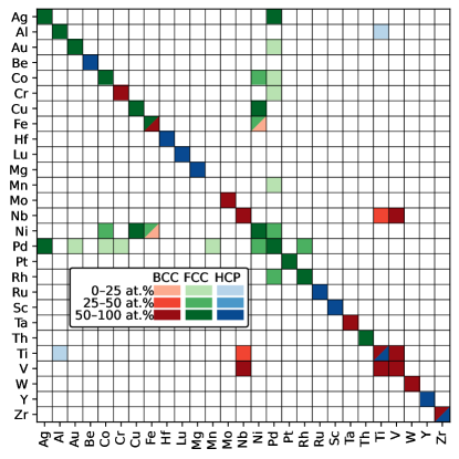
Table 1 lists the activation energies for the pure metals organized by crystal structure. The activation energies for the metals depend heavily on the crystal structures, and the BCC metals have 0.24 eV smaller activation energies on average than the close-packed FCC and HCP metals. For HCP metals where the reported diffusion was anisotropic, we use the effective activation energy by taking an average over the activation energies in directions parallel and perpendicular to the basal plane. Note that Fe has activation energies for hydrogen diffusion in both BCC and FCC crystal structures, while Ti and Zr have activation energies in both BCC and HCP crystal structures. The mean activation energy is 0.31 eV with a standard deviation of 0.15 eV. While the pure elements shown in Table 1 have a larger mean of 0.38 eV and a larger standard deviation of 0.20 eV, the opposite is true for the binary alloys, which have a mean of 0.29 eV and a standard deviation of 0.11 eV, so the alloys not only cover a smaller composition range, but also a smaller range of activation energies.
| BCC | (eV) | FCC | (eV) | HCP | (eV) |
|---|---|---|---|---|---|
| Cr | 0.020 [47] | Pd | 0.236 [48, 49, 50, 51] | Mg | 0.250 [52] |
| V | 0.046 [66, 68, 67] | Pt | 0.264 [53, 54] | Zr | 0.427[55, 56, 57, 58] |
| Fe | 0.069 [60, 61] | Au | 0.273 [77, 62] | Hf | 0.464 [63, 64] |
| Nb | 0.098 [66, 65, 67, 68, 69] | Ag | 0.312 [87] | Y | 0.496 [88, 89, 90] |
| Ta | 0.152 [67, 70, 68, 69, 71] | Cu | 0.375 [77, 78, 81, 79, 80] | Ti | 0.508 [72, 63] |
| Mo | 0.185 [73, 74, 75, 76] | Ni | 0.413 [82, 83, 80, 81, 84, 85, 86] | Sc | 0.540 [59] |
| Ti | 0.273 [91, 72] | Th | 0.419 [92] | Lu | 0.575 [93] |
| Zr | 0.361 [56] | Al | 0.452 [94, 95] | Be | 0.611 [96] |
| W | 0.387 [97] | Fe | 0.460 [98] | Ru | 0.763 [31] |
| Co | 0.507 [99] | ||||
| Rh | 0.892 [14] |
Fig. 2 shows the properties that are used as input into our machine learning models and their correlations with the hydrogen activation energy. For the binary alloys, no alloy properties are included, but we use the averages of the elemental properties weighted by the atomic percentages. These properties come from two sources: theoretical models of interstitial diffusion and broader elemental and stoichiometric properties from the MAGPIE database [45]. For the MAGPIE features we also include the standard deviations of the features, and for metals, the standard deviations are set to 0. By including these two types of features, we allow our model to use known proponents to hydrogen diffusion, while also picking out new features. We include features from models of hydrogen diffusion: the electronic specific heat [100], thermal conductivity [100], and the 15 features [101, 102, 103, 104, 105, 106, 107, 108, 109] that were used to model C, O, and B interstitial diffusion in metals [35]. The electronic specific heat coefficient of the metal is included because it has been found by Arnoult and McLellan [110] to have an empirical linear relationship with the relative partial enthalpy of hydrogen solubility. The thermal conductivity allows us to take into account phonon modes in the metal. A detailed description of the MAGPIE features and their sources is found in the original paper [45]. The method of counting valence electrons differs between MAGPIE and Zeng et al. [35], so we have included both, and the MAGPIE version is denoted with an asterisk. The MAGPIE version defines the valence electrons by excluding any noble gas electron configurations from the total electrons, while Zeng et al. only count the outermost shell. While we have renamed most features so that their names are intuitive, four features are more difficult to understand. The stoichiometric 5-norm is defined as where is the atomic fraction of each element, is the absolute difference of the electron density at the boundary of the Wigner-Seitz cell between the host and hydrogen, is the ratio of the Debye temperature to the melting temperature, and is obtained from an empirical elastic model [111], which is a simplified version of Eqn. 1:
| (3) |
where all the variables are the same as was defined in Eqn. 1. To reduce the impact of multicollinearity on our models, we remove 11 features with correlations greater than 0.95 with another feature. When two features were correlated strongly, we kept the feature with the strongest correlation with the activation energy. We also remove constant features that are the same for all entries in the database. In the middle panel of Fig. 2, we show the Pearson correlation between each feature and the activation energy. The packing factor has the largest correlation with the activation energy with a correlation value of 0.54. For input into our machine learning models, we scale all features so that they have a mean of 0 and a standard deviation of 1.
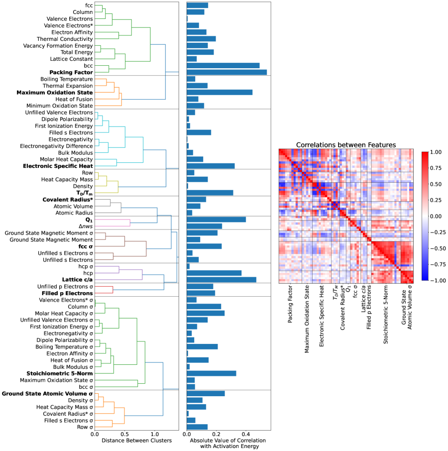
We combine our features into ten groups using their correlations in Fig. 2, and the three largest groups (packing factor, electronic specific heat, and stoichiometric 5-norm) roughly split the features into structural and energetic, electronic, and alloy standard deviation property groups. The hierarchical tree shown in the left panel forms correlated feature groups using Ward’s minimum variance method to minimize the variance between elements in the same cluster [112]. Groups are formed by choosing a threshold, which we choose to be 1 (the maximum value of the distance metric between two elements). This distance threshold creates a suitable number of groups to improve interpretability of our features. Having too many groups is difficult to interpret, while too few groups makes each group too broad. To define the distance, we used the Spearman rank correlation to take into account any nonlinear, monotonic relationships between the features as the majority of our models are nonlinear. Shown in the right panel, the Spearman rank correlations in the upper right triangle are also stronger than their Pearson counterparts in the bottom left, which allows us to form groups with stronger intra-group correlations. We named each of the 11 groups after the representative feature with the strongest absolute value of the correlation with the activation energy. The three largest groups are “stoichiometric 5-fold” (14 features), “packing factor” (11), and “electronic specific heat” (9). The stoichiometric 5-fold group contains the standard deviations of the features that measure how the elemental properties vary, the packing factor group contains energetic and structural information, and the electronic specific heat group contains electronic properties. The standard deviations of the properties are spread over 5 out of the 11 groups (fcc , lattice , filled electrons, stoichiometric 5-fold, and ground state atomic volume ) in the bottom half of Fig. 2. These groups improve interpretability of our features by reducing the feature set.
II.2 Machine Learning Models
In this paper, we use six different machine learning models that work well on small data sets: -nearest neighbors, Gaussian process, random forest, gradient boosting, positive ElasticNet, and Bayesian Ridge. All models are trained using scikit-learn [113], a Python package for machine learning.
II.2.1 -Nearest Neighbors
The -nearest neighbors models find the closest training samples from an input data point, and then assign the new point a linear combination of its neighbors’ values [114, 115]. The distance between points used is the Euclidean distance. Because it is an algorithm that uses all of its training data and does not build a model, -nearest neighbors models do not generalize well to unseen data. They also suffer from the curse of dimensionality, where the amount of data needed to get accurate predictions increases exponentially with the dimensionality of the data [116]. We choose to optimize two hyperparameters: weighting scheme and number of neighbors. The two weighting schemes, uniform or distance, determine how to weigh the neighbors’ activation energies when assigning one to a new point. The uniform weighting scheme gives equal weights to all neighbors, while the distance weighting scheme assigns a weight that is proportional to the distance to the new point.
II.2.2 Gaussian Process
The Gaussian process model creates a prior distribution over possible functions, then uses Bayesian interference to update the posterior based on new training data [117, 118]. These models define the covariance of their prior distribution using kernels, and train a Gaussian posterior distribution over functions whose mean is used for predictions. We assume that the prior distributions for the noise is the Gaussian and the prior distribution for the weights is where is the variance, is the identity matrix and is a covariance matrix. Given a function where is an input data point, the model is described as:
We then combine the into a matrix that includes all the training data and then define the posterior function for the weights as:
| (4) |
where and is the target output. Instead of explicitly defining the basis functions, we use the kernel trick to make the calculations faster. For our models, we choose to use two different types of kernels: white kernels and radial basis function (RBF) kernels. The noise level on the white kernel denotes the size of the random noise fluctuations in the data, while the RBF kernel’s length scale denotes the length scales of the fluctuations. While the actual value of these hyperparameters is optimized by the model, we choose a starting value with nested cross validation to reduce the chances of falling into a local minimum where all deviation in the activation energies is considered random noise.
II.2.3 Random Forest
Random forest models are ensemble methods that take an average over independent decision trees [119]. Each tree is trained on a random sample of the complete dataset and acts as a weak learner. Even though each individual decision tree often overfits, using random samples of the data and averaging over the trees allow errors to cancel out. The hyperparameters of a random forest model are the total number of trees and the maximum depth of each tree.
II.2.4 Gradient Boosting
Another ensemble method, gradient boosting models build each tree sequentially, so that each tree reduces the bias of the final combined estimator [120, 121]. This allows it to perform better than the random forest model where the trees are independent. Gradient boosting models, which work well on small data sets, have been used to design explainable models for other material properties like thermodynamic properties of hydride formation in alloys and intermetallics [42] and for interstitial diffusion, not including hydrogen, in metals [35]. We optimized the learning rate of each tree and the complexity of the trees through the number of estimators and maximum depth.
II.2.5 Positive ElasticNet
The positive ElasticNet model is an ordinary least squares estimator with an additional Ridge and lasso penalty [122]. It assumes that the models are linear, while also penalizing the size and number of non-zero coefficients, which makes it more stable than a simple least squares estimator. To make sure that all predicted activation energies are positive and therefore physical, we further constrain all coefficients to be positive, scale all the features between 0–1, and include a reversed version of all the features so that for each feature , we include a new feature where . This allows us to include negative correlations between our features and the activation energy, while still constraining the activation energies to be positive. We choose to enforce positive results by using positive coefficients instead of using a non-linear transformation to maintain its interpretability. A log transformation would turn the ElasticNet model into a product of terms, instead of a sum, reducing the physical relevance. We optimize the size of the Ridge penalty and the ratio between the Ridge and lasso penalty.
II.2.6 Bayesian Ridge
Bayesian Ridge models are probabilistic, linear models that tune the weights and regularization parameters from an uninformative prior [123] where the prior distributions for the noise is a Gaussian and the prior distribution for the weights is where is the variance and is the identity matrix. Given an input matrix of features and a desired output , the posterior distribution for the weights is defined as
| (5) |
where . Note that these are identical to the Gaussian process except that the matrix of basis functions is replaced with simply . The four hyperparameters , , , and define the prior Gamma distributions from which the regularization parameters are chosen. In this work, we use for the four hyperparameters to guarantee a flat, uninformative prior distribution so that the expectation-maximization algorithm can adjust the precision of the weights and noise without bias. Because no negative predictions were made, we did not add any additional constraints to guarantee positive activation energy predictions for the Bayesian Ridge models.
III Results
III.1 Model Fitting
| Model | Hyperparameter | Start | End | Step Size | Optimal value |
|---|---|---|---|---|---|
| K-Nearest Neighbors | Number of Neighbors | 1 | 8 | 1 | 2 |
| Weighting Scheme | Distance, Uniform | Distance | |||
| Gaussian Process | Length Scale (RBF) | 5 | 50 | 5 | 35 |
| Noise Level (white) | |||||
| Random Forest | Number of Estimators | 40 | 90 | 10 | 70 |
| Maximum Depth | 3 | 14 | 1 | 10 | |
| Gradient Boosting | Learning Rate | 0.1 | 1 | 0.1 | 0.3 |
| Number of Estimators | 100 | 170 | 10 | 150 | |
| Maximum Depth | 2 | 8 | 1 | 2 | |
| Positive ElasticNet | Ridge Penalty | 1 | |||
| ratio | 0.025 | 1.0 | 0.0125 | 0.05 | |
| Bayesian Ridge | |||||
In order to ensure that our results are independent of the chemistry of our training set, we tune the hyperparameters (see Table 2) via nested cross validation by leaving out all data that contain a certain element (alloy split) [124] at each iteration and then choosing the optimal hyperparameter as the median over all iterations. Within each iteration, we perform a 80–20% split and perform a grid search to find the hyperparameters that lead to the smallest mean squared error between the predicted and experimental activation energies. The start and end values are the upper and lower bounds, and each hyperparameter varies by step size increments. Because the Bayesian Ridge’s hyperparameters define the prior Gamma distributions from which the optimal values are chosen, we choose the values manually instead of through nested cross validation. We also performed a sensitivity analysis of our hyperparameters shown as Table S1 of the Supplemental Material 111See Supplemental Material at [URL will be inserted by publisher] for hyperparameter sensitivity analysis, linear models for deuterium and tritium activation energies, and the grouping analysis applied to the SHAP values, and other than the learning rate for the gradient boosting tree model, the RMSEs on the testing data changed by less than 10 meV when all other hyperparameters were increased or decreased by one step size. Decreasing the learning rate by a single step (0.1) led to the RMSE decreasing by 19 meV as smaller learning rates can reduce the amount of overfitting, thus improving predictions on the test set. To make sure that no positive bias is introduced to our error predictions, the original hyperparameter is used. As an additional measure of the possible bias in our hyperparameter choice, we recalculated the test RMSEs for the alloy split so that all test data is not used to also select the hyperparameter and found a less than 7 meV deviation between the two RMSEs as shown in Table S2 of the Supplemental Material [125]. This implies that there is no positive bias introduced from reusing data, and that our models are not overfitting to the hyperparameters.
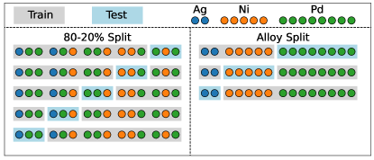
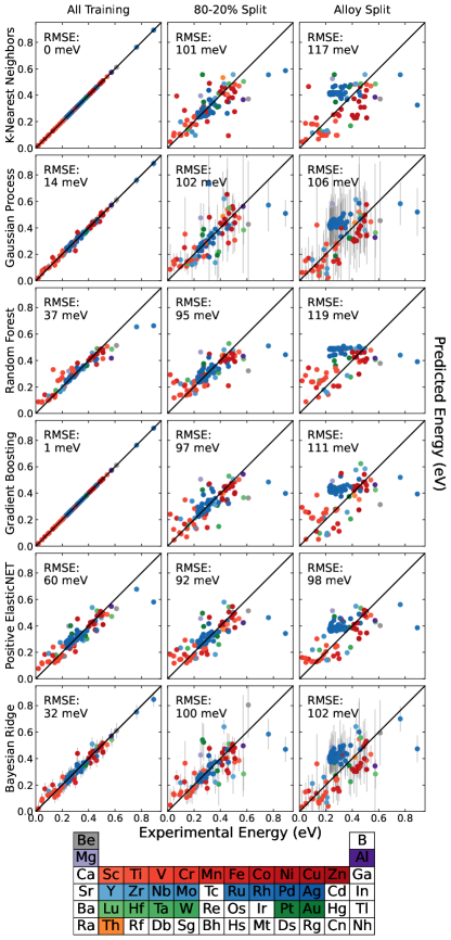
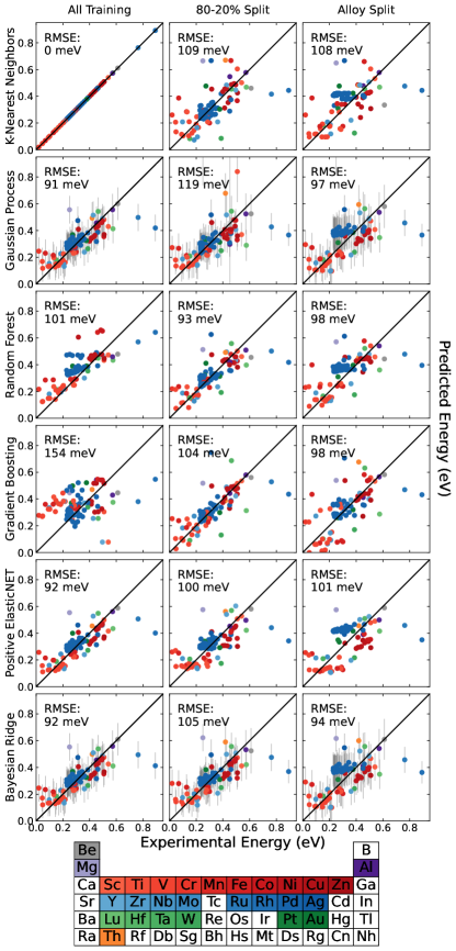
Using our optimal hyperparameters, we train six models with three different train-test splits and obtain similar root-mean-squared-errors (RMSEs) for the 80–20% split and alloy split; the test RMSE of the alloy split is, on average, 18 meV higher than the 80–20% split. A schematic detailing the two train-test splits is shown in Fig. 3. Each model is trained 100 times (with different random splits for the 80–20% train-test split), and the average testing RMSEs are reported. The error of the training predictions (leftmost column of Fig. 4) shows the ideal performance of our models when it is trained on the entire dataset. In the middle and right columns of Fig. 4, we plot only predictions on the test set, and no training data is shown. For the alloy split, shown in the right column of Fig. 4, we choose to plot only the binary alloy predictions from the model where the dominant element is removed from training (or the average of the two predictions for equiatomic systems) instead of plotting both predictions from each of the alloy splits. The 80–20% train-test split has smaller RMSEs than the alloy split for all six models due to significantly more accurate alloy predictions because of similar training and testing sets. Alloy activation energy predictions have 85 meV smaller RMSEs on average when we use the 80–20% split instead of the alloy split, while elemental predictions have 6 meV larger RMSEs. The Gaussian proces, positive ElasticNet, and Bayesian Ridge model have two smallest RMSEs for the alloy split and are the best at generalizing to unseen data. This is because these three models are the only continuous models that have in-built regularization and reduce overfitting, especially with the small database used in this study. The Gaussian process model also deals effectively with noisy data by controlling the length scale of the RBF kernel, which ensures that small fluctuations below this length scale in the training data are ignored [123]. These average RMSEs are greater than the errors from typical DFT calculations for hydrogen diffusion which usually lie within a few 10s of meV from experimental values [13, 14, 15, 16, 17, 18, 19, 20, 21, 22, 23, 24, 25, 26, 27, 28, 29, 30]. Because the average RMSEs for the models are greater than the isotope effect, our models are unable to accurately predict activation energies for deuterium and tritium. Because more complex models will overfit to the small amount of deuterium and tritium data, we instead fit a separate linear model with a single feature in Section S2 of the Supplemental Material [125].
Even though the activation energies are predicted with relatively small RMSEs, our machine learning models are limited because they overemphasize crystal-dependent features over element-dependent features for the alloy train-test split (right column of Fig. 4). This is most obvious for the FCC Pd alloys and elemental Rh, which are predicted to have activation energies close to the mean for their crystal structure (0.34 eV) but in reality, their activation energies are the lower and upper bounds. Pd and its alloys, which consist of a third of the total database, have activation energies that are systematically overestimated especially on the Pd-rich side with smaller activation energies. Therefore, when the Pd alloys are excluded from training in the alloy-split validation method, the models learn to predict values that are closer to the average for their crystal structure even though it leads to incorrect predictions on the Pd test set. This leads to the prominent ‘clump’ of blue Pd alloys in the range of 0.36–0.46 eV in Fig. 4. Rh, an outlier with the largest activation energy, is drastically underestimated and has the largest errors for all six models. This behavior is because strong correlations between the activation energy and the packing factor can dominate effects that are only significant for a few specific elemental systems, such as Pd and Rh having smaller atomic radii compared to other elements in their row, which has been shown to have an effect on the speed of solute diffusion in Ni [126]. This limitation of our machine learning models is likely due to a lack of other metals or alloys in our training database with such extreme activation energies.
III.2 Uncertainty Quantification
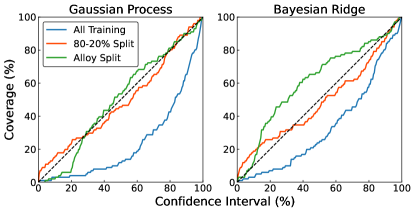
For models which explicitly quantify uncertainty (Gaussian Process and Bayesian Ridge), it is important to understand the reliability of these uncertainty estimates, especially if one is predicting new materials containing previously seen elements (80–20% test split) or entirely unseen elements (alloy test split). The uncertainty quantification in Fig. 5 reveals that the predicted standard deviations for the Gaussian process model accurately predicts the observed errors, but the Bayesian Ridge model’s predicted standard deviations are only reliable on testing data that is similar to its training data. Instead of a single solution, the models fit a posterior distribution described in Eqn. 4 and Eqn. 5 whose standard deviations depend heavily on hyperparameters that are learned through the data—either the noise level on the white kernel for the Gaussian process or the precision of the weights and noise for the Bayesian Ridge. The average sizes of the predicted standard deviation for the Gaussian process model are 27, 80, and 172 meV for the all training, 80–20% split, and alloy split respectively, while for the Bayesian Ridge model, the average standard deviations are 48, 72, and 120 meV for the three train-test splits. As expected, the uncertainty increases for train-test splits with different elemental compositions than the training data. In Fig. 5, we perform this analysis by comparing the predicted standard deviations from the model uncertainty quantification with the observed errors by plotting the coverage percent, which indicates the fraction of data points within a given confidence interval. The confidence intervals are calculated assuming that the predicted standard deviations are accurate. If the p-values are uniformly distributed (the dashed line in Fig. 5), then the observed errors sample the same Gaussian distribution as the predicted standard deviations. Curves that lie above the line suggest that observed errors sample a broader Gaussian than the predicted standard deviations, so the predicted error bars are too small. For curves that lie below the line, the observed errors are too large, and the predicted standard deviations are too conservative. The all training models both overestimate the error, and in both models, less than 10% of the predicted values (3% for Gaussian process and 7% for Bayesian Ridge) fall more than 1.28 standard deviations away (the 20% confidence interval) from the true experimental value. This likely arises because the models have large amounts of variance, and there is a wide distribution of possible functions with low bias, so the mean ends up being close to the true value [116]. While both models’ predicted standard deviations deviate from the observed errors for the alloy split case, the predicted standard deviations on the 80–20% split for both the Gaussian process and Bayesian Ridge agree strongly. The Gaussian process slightly overestimates the error, and almost all of its observed errors are within one predicted standard deviation, but it recovers to the ideal distribution after the 30% confidence interval. On the other hand, the Bayesian Ridge model heavily underestimates the observed errors for the alloy split. This can be understood by interpreting the Bayesian Ridge model as a simpler Gaussian process model whose kernel choice forces it to only use a limited prior. This makes the posterior distribution too concentrated, which leads to overconfidence as it cannot recognize that the new data are different than its training data [116, 127]. Therefore, the Gaussian process model’s predicted standard deviations can be trusted with new elemental compositions, but the Bayesian Ridge’s predictions can only be trusted for similar data.
III.3 Model Explainability
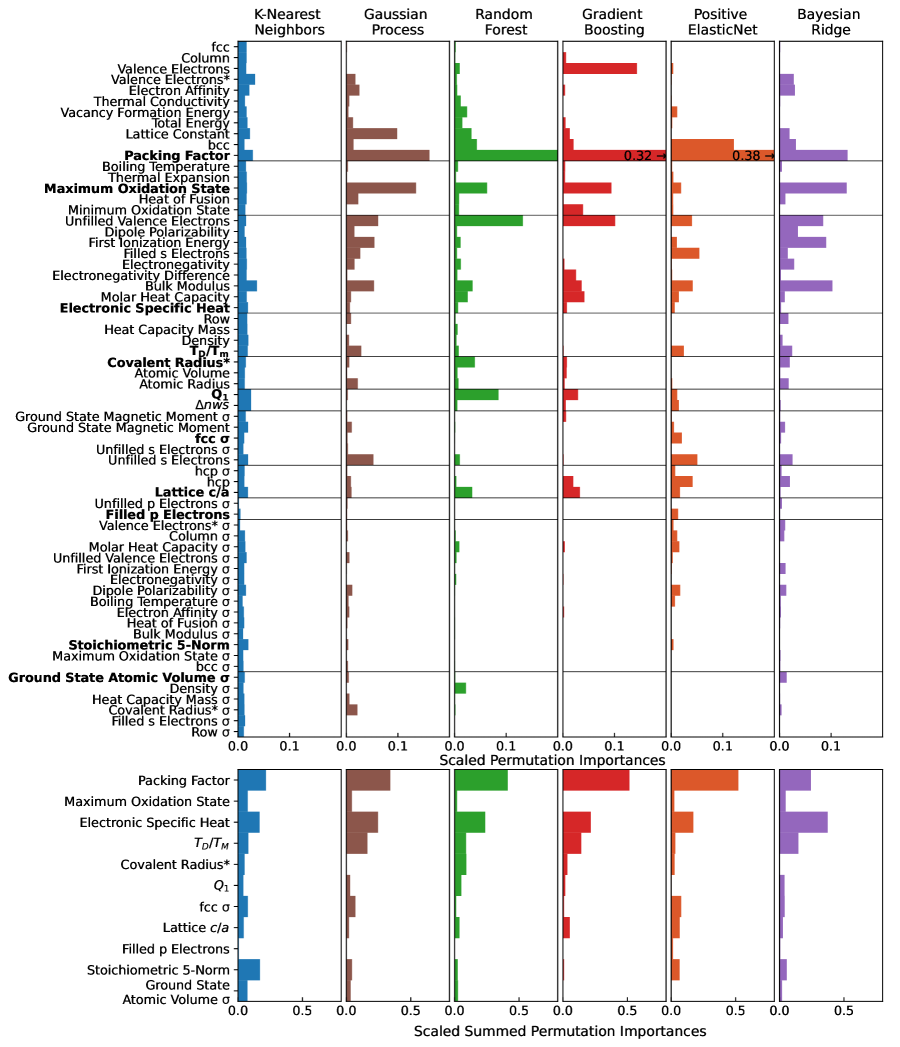
Strong correlations between features lead to wide variations of feature importances calculated for different models, making physical interpretation of the models difficult as shown in Fig. 6. We use the permutation importance, which measures how much the value changes after shuffling the features, to measure the importance of each feature. Scaling the permutation importances within each model to sum to 1 enables comparisons between the models. Even though the importance is measured using the same metric for all six models, we find large variation in the feature importances; just listing the top three features from each model leads to a total of ten different features – none of which are consistent for all the models. The models agree most when identifying the importance of the packing factor, as it is the most important feature for all except for the -nearest neighbors model. The -nearest neighbors model assigns nearly equal importances to all features due to it being a non-parametric model that only takes into account distances between points rather than a model-building method. This wide variation in the importance of individual features arises from correlated material properties and makes interpretation difficult, but after grouping the features using the greedy algorithm shown in Fig. 2, we find that specific feature groups are selected. Similar behavior can be seen in previous work on modeling solute diffusion in metals [36, 124], which saw varying feature importances by using different models and cross validation techniques. Thus, it becomes clear that using the individual permutation importances (or other metrics of feature importances like the Shapley additive explanations [128] shown in S3 of the supplementary information [125]) for individual features do not offer as much information on important features as grouping analyses do.
The feature groups in Fig. 6 lead to stronger agreement between the models, and when we then sum the importances to rank the groups, the two most important ones are the packing factor and electronic specific heat. Here, we ignore the -nearest neighbor model because its grouped importance is ultimately just a measure of the group size, but the other five models agree that the packing factor and electronic specific heat are the two most important groups. Agreement depends on sparsity as more sparse models, like the gradient boosting tree and positive ElasticNet models, conclude that the packing factor group is more important, while less sparse models, like the Gaussian process and Bayesian Ridge models, assign the packing factor and electronic specific heat more similar importances. The Bayesian Ridge model is the only model to swap the ranks of the packing factor and the electronic specific heat groups because it assigns a large importance to many features in the same group. The packing factor group contains energetic and structure information like the vacancy formation energy and lattice constant, which are directly related to hydrogen diffusion. While the packing factor and crystal structure determine what kind of interstitial sites are available to form the diffusion pathways, the vacancy formation energy has an strong empirical correlation with the activation energy [106]. The electronic specific heat feature group, which contains electronic properties and the bulk modulus, is dominated by features that measure hydrogen’s interaction with the bulk. The top two groups are followed distantly by the maximum oxidation state, then the , lattice , stoichiometric 5-norm, and fcc groups, which all have effectively the same importances.
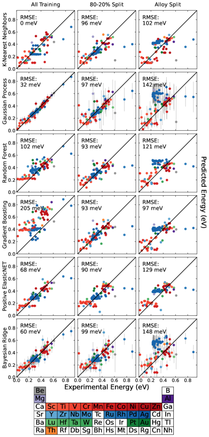
A reduced feature set with only each group’s representative feature (Fig. 7) has RMSEs similar to the fits using the whole feature set while using only features in the top two groups (Fig. 8) has significantly larger RMSEs. Out of the three feature sets, trained models using the representative feature set have the best transferability because the RMSEs for the alloy split are the smallest. This is because while the representative feature set is the smallest, the removed features are correlated with the representative feature that is kept, so little information is lost. The top two groups feature set, on the other hand, has significantly worse predictions on the alloy split, especially for the Gaussian process, positive ElasticNet, and Bayesian Ridge models. This is a result of extremely poor predictions of the activation energies for the Pd alloys. Due to the larger importances for the maximum oxidation state group for the Gaussian process and Bayesian Ridge models, shown in Fig. 6, they rely more strongly on the removed information than the others, so they are more negatively impacted by reducing the feature set to only the top two groups. For the positive ElasticNet model, we reoptimized the hyperparameters using the same nested cross validation technique for the two smaller feature subsets. If we use the same hyperparameters as we do for the full feature set, we observe significant banding of alloy predictions for both the 80–20% train-test split and the alloy split due to overzealous regularization as the size of the Ridge and Lasso penalties are too large for the smaller feature set, which leads to too many ignored features and small coefficients. This suggests that any model for the activation energy of hydrogen in metals should contain at least one feature from each group.
IV Discussion
In this paper, we create a database and fit six different machine learning models to predict hydrogen diffusion activation energy in metals and random binary alloys and achieve smaller errors than a similar, earlier machine learning model for interstitial diffusion [35]. On the testing data, these models obtain a 92–102 meV RMSE for a random 80–20% train-test split, and a larger 105–124 meV RMSE for an alloy leave-one-group-out train-test split, which measures how the model performs on unseen elements. These errors are smaller in magnitude than a gradient boosting model for interstitial diffusion (C, O, B, and N) by Zeng et al. [35] who obtained a final RMSE of 311 meV on testing data even though we have similar elemental compositions and the sizes of our databases were similar. Because Zeng et al. only used random train-test splits, which we find to have smaller RMSEs than the grouped alloy split by the host metal, and used a smaller test set, we expect this RMSE to be a underestimation of the error when applying the model to materials with elements not existing in the training data. This difference in the RMSEs is likely because the range of their activation energies 0.19–2.45 eV was approximately 3 times larger than our range of 0.02–0.89 eV because they were dealing with multiple solute types.
Comparisons between our importance analysis and other analytic and machine learning models show that due to hydrogen’s small size, features that are included in Ferro’s elastic model [32] are missing; otherwise, the involved material properties agree with the other models. By training our machine learning models on the downselected feature sets, our machine learning models behave akin to analytic models and can be analyzed similarly. The interstitial model in Zeng et al. [35] obtained four important features for predicting non-hydrogen interstitial diffusion: electronegativity difference, total energy, (see Eqn. 3) and thermal expansion. Other than , these features fall in the three most important feature groups for our hydrogen diffusion model (electronic specific heat, packing factor, and maximum oxidation state), pointing to fundamental similarities between hydrogen diffusion and that of other small interstitial atoms. However, contains 3% of the overall importance, and the other material property that appears in both our machine learning model and Ferro’s elastic model [32] shown in Eqn. 1, , is equally unimportant and has less than 3% of the overall importance. This implies that Ferro’s elastic model is less applicable to predicting hydrogen diffusion, possibly due to its small size leading to smaller lattice distortions. The quantum mechanical model by Flynn and Stoneham [34] in Eqn. 2 has fewer directly overlapping features with our machine learning models, but similar physical and electronic features appear. The lattice constant determines the jump distance in Flynn’s model, and the radius of the Debye sphere , or screening length, is directly tied to the strength of electronic interactions between the hydrogen and the host metal — similar to the features found in the electronic specific heat feature group, which contains electronic properties and the bulk modulus. Within this group, the electronegativity appears in the Miedema model [129], which has been used to calculate the enthalpy of formation [130, 131, 132] and the hydrogen content [133] for metal hydrides, and the bulk modulus measures the compressibility of a hydrogen atom into a crystal. Therefore, while electronic interactions between the hydrogen and the bulk remain important for predicting hydrogen diffusion, due to hydrogen’s small size, elastic models are less applicable.
In this work we construct a database of material properties for predicting hydrogen diffusivity, and grouped features to interpret ML models on this task. Not only will our machine learning models enable predictions of hydrogen diffusion in metals or random alloys that have not previously been measured in experiments due to the wide variety of elements included in our database, but the new physical insights into the activation energies of hydrogen diffusion in metals and binary alloys will help streamline the process for materials discovery for fast-diffusing or slow-diffusing materials for hydrogen containment or transportation. For ternary or quaternary alloys, even though they were not directly included in the training data, we anticipate that our machine learning models will work within the estimated error bars, but more importantly, the same features that were important for the metal and binary alloys should still be physically meaningful to screen for ideal hydrogen diffusivities. Because the material properties used in this study are easy to measure either experimentally or using DFT, the results will enable data-driven screening of materials without needing explicit measurements of the hydrogen diffusion. Additionally, the technique of grouping the features into correlated feature groups before analyzing feature importances can be applied to other material property predictions, namely for diffusion and other temporal properties, and enable rapid screening for other desired properties.
Acknowledgements.
This work was supported by by the National Science Foundation Graduate Research Fellowship under Grant No. 1746047 (G.L.). The authors gratefully thank Dr. Rick Karnesky, Josh Vita, and Luke Wirth for the helpful comments and discussions. This work was supported by the Laboratory Directed Research and Development (LDRD) program at Sandia National Laboratories. Sandia National Laboratories is a multimission laboratory managed and operated by National Technology & Engineering Solutions of Sandia, LLC, a wholly owned subsidiary of Honeywell International Inc., for the U.S. Department of Energy’s National Nuclear Security Administration (DOE/NNSA) under contract No. DE-NA0003525. This written work is authored by an employee of NTESS. The employee, not NTESS, owns the right, title and interest in and to the written work and is responsible for its contents. Any subjective views or opinions that might be expressed in the written work do not necessarily represent the views of the U.S. Government. The DOE will provide public access to results of federally sponsored research in accordance with the DOE Public Access Plan.References
- Züttel et al. [2010] A. Züttel, A. Remhof, A. Borgschulte, and O. Friedrichs, Hydrogen: the future energy carrier, Philosophical Transactions of the Royal Society A: Mathematical, Physical and Engineering Sciences 368, 3329 (2010).
- Irani [2002] R. Irani, Hydrogen storage: High-pressure gas containment., MRS Bulletin 27, 680 (2002).
- Song and Curtin [2013] J. Song and W. A. Curtin, Atomic mechanism and prediction of hydrogen embrittlement in iron, Nature Materials 12, 145 (2013).
- Schapbach and Zuttel [2001] L. Schapbach and A. Zuttel, Hydrogen-storage materials for mobile applications., Nature 414, 353 (2001).
- Schneemann et al. [2018] A. Schneemann, J. L. White, S. Kang, S. Jeong, L. F. Wan, E. S. Cho, T. W. Heo, D. Prendergast, J. J. Urban, B. C. Wood, M. D. Allendorf, and V. Stavila, Nanostructured Metal Hydrides for Hydrogen Storage, Chemical Reviews 118, 10775 (2018).
- Sakintuna et al. [2007] B. Sakintuna, F. Lamari-Darkrim, and M. Hirscher, Metal hydride materials for solid hydrogen storage: A review, International Journal of Hydrogen Energy 32, 1121 (2007).
- Aguey-Zinsou and Ares-Fernández [2010] K.-F. Aguey-Zinsou and J.-R. Ares-Fernández, Hydrogen in magnesium: New perspectives toward functional stores., Energy and Environmental Science 3, 526 (2010).
- Webb [2015] C. Webb, A review of catalyst-enhanced magnesium hydride as a hydrogen storage material., Journal of Physics and Chemistry of Solids 84, 96 (2015).
- Yartys et al. [2019] V. Yartys, B. Denys, R.V.and Hauback, M. Lototskyy, E. Akiba, R. Albert, M. Felderhoff, V. Antonov, M. Kuzovnikov, J. Ares, M. Baricco, N. Bourgeois, J.-C. Crivello, F. Cuevas, J.-M. Joubert, M. Latroche, C. Buckley, T. Humphries, M. Paskevicius, M. Sofianos, J. Bellosta von Colbe, M. Dornheim, D. Grant, A. Stuart, G. Walker, I. Jacob, T. Jensen, L. de Jongh, P.E.and Pasquini, L. Popilevsky, V. Skripnyuk, E. Rabkin, H. Wang, M. Zhu, and C. Webb, Magnesium based materials for hydrogen based energy storage: Past, present and future., International Journal of Hydrogen Energy 44, 7809 (2019).
- Adams and Chen [2011] B. D. Adams and A. Chen, The role of palladium in a hydrogen economy., Materials Today 14, 282 (2011).
- Kirchheim and Pundt [2014] R. Kirchheim and A. Pundt, Hydrogen in Metals, in Physical Metallurgy (Elsevier, 2014) pp. 2597–2705.
- Wipf [2001] H. Wipf, Solubility and Diffusion of Hydrogen in Pure Metals and Alloys, Physica Scripta T94, 43 (2001).
- Kamakoti [2003] P. Kamakoti, A comparison of hydrogen diffusivities in Pd and CuPd alloys using density functional theory, Journal of Membrane Science 225, 145 (2003).
- Baykara [2004] S. Baykara, Theoretical evaluation of diffusivity of hydrogen in palladium and rhodium, International Journal of Hydrogen Energy 29, 1631 (2004).
- Jiang and Carter [2004] D. E. Jiang and E. A. Carter, Diffusion of interstitial hydrogen into and through bcc Fe from first principles, Physical Review B 70, 064102 (2004).
- Bhatia and Sholl [2005] B. Bhatia and D. S. Sholl, Quantitative assessment of hydrogen diffusion by activated hopping and quantum tunneling in ordered intermetallics, Physical Review B 72, 224302 (2005).
- Wimmer et al. [2008] E. Wimmer, W. Wolf, J. Sticht, P. Saxe, C. B. Geller, R. Najafabadi, and G. A. Young, Temperature-dependent diffusion coefficients from ab initio computations: Hydrogen, deuterium, and tritium in nickel, Physical Review B 77, 134305 (2008).
- Duan et al. [2010] C. Duan, Y.-L. Liu, H.-B. Zhou, Y. Zhang, S. Jin, G.-H. Lu, and G.-N. Luo, First-principles study on dissolution and diffusion properties of hydrogen in molybdenum, Journal of Nuclear Materials 404, 109 (2010).
- Connétable et al. [2011] D. Connétable, J. Huez, É. Andrieu, and C. Mijoule, First-principles study of diffusion and interactions of vacancies and hydrogen in hcp-titanium, Journal of Physics: Condensed Matter 23, 405401 (2011).
- Liu et al. [2012] Y.-L. Liu, S. Jin, L. Sun, and C. Duan, First-principles investigation on diffusion and permeation behaviors of hydrogen isotopes in molybdenum, Computational Materials Science 54, 32 (2012).
- Lu and Zhang [2013] Y. Lu and P. Zhang, First-principles study of temperature-dependent diffusion coefficients: Hydrogen, deuterium, and tritium in -Ti, Journal of Applied Physics 113, 193502 (2013).
- Fernandez et al. [2015] N. Fernandez, Y. Ferro, and D. Kato, Hydrogen diffusion and vacancies formation in tungsten: Density Functional Theory calculations and statistical models, Acta Materialia 94, 307 (2015).
- Tafen [2015] D. N. Tafen, First-principles-based kinetic Monte Carlo studies of diffusion of hydrogen in Ni–Al and Ni–Fe binary alloys, Journal of Materials Science 50, 3361 (2015).
- Han et al. [2016] Q.-F. Han, Z.-Y. Zhou, Y. Ma, and Y.-L. Liu, A comparative investigation of the behaviors of H in Au and Ag from first principles, Modelling and Simulation in Materials Science and Engineering 24, 045009 (2016).
- Yang et al. [2016] X.-Y. Yang, Y. Lu, and P. Zhang, First-principles study of the stability and diffusion properties of hydrogen in zirconium carbide, Journal of Nuclear Materials 479, 130 (2016).
- Liu et al. [2017] L. Liu, J. Wang, Y. He, and H. Gong, Solubility, diffusivity, and permeability of hydrogen at PdCu phases, Journal of Membrane Science 542, 24 (2017).
- Liu et al. [2018] L. Liu, J. Wang, J. Qian, Y. He, H. Gong, C. Liang, and S. Zhou, Fundamental effects of Ag alloying on hydrogen behaviors in PdCu, Journal of Membrane Science 550, 230 (2018).
- Oliveira et al. [2019] R. R. Oliveira, B. N. Tenorio, and A. B. Rocha, Ab initio study of diffusion of hydrogen, silver and lithium in PbS and Ag2S, Computational Materials Science 166, 75 (2019).
- Yang and Wirth [2019] L. Yang and B. D. Wirth, First-principles study of hydrogen diffusion and self-clustering below tungsten surfaces, Journal of Applied Physics 125, 165105 (2019).
- Connétable [2019] D. Connétable, Theoretical study of the insertion and diffusivity of hydrogen in the Ti3Al-D019 system: Comparison with Ti-hcp and TiAl-L10 systems, International Journal of Hydrogen Energy 44, 32307 (2019).
- Onwudinanti et al. [2020] C. Onwudinanti, G. Brocks, V. Koelman, T. Morgan, and S. Tao, Hydrogen diffusion out of ruthenium—an ab initio study of the role of adsorbates, Physical Chemistry Chemical Physics 22, 7935 (2020).
- Ferro [1957] A. Ferro, Theory of diffusion constants in interstitial solid solutions of b.c.c. metals, Journal of Applied Physics 28, 895 (1957).
- McNeil [1965] M. B. McNeil, Calculation of Activation Energies for Interstitial Diffusion by a Simple Elastic Model, Journal of Applied Physics 36, 2328 (1965).
- Flynn and Stoneham [1970] C. P. Flynn and A. M. Stoneham, Quantum Theory of Diffusion with Application to Light Interstitials in Metals, Physical Review B 1, 3966 (1970).
- Zeng et al. [2018] Y. Zeng, Q. Li, and K. Bai, Prediction of interstitial diffusion activation energies of nitrogen, oxygen, boron and carbon in bcc, fcc, and hcp metals using machine learning, Computational Materials Science 144, 232 (2018).
- Wu et al. [2017] H. Wu, A. Lorenson, B. Anderson, L. Witteman, H. Wu, B. Meredig, and D. Morgan, Robust FCC solute diffusion predictions from ab-initio machine learning methods, Computational Materials Science 134, 160 (2017).
- Wei et al. [2021] Z. Wei, J. Yu, Y. Lu, J. Han, C. Wang, and X. Liu, Prediction of diffusion coefficients in fcc, bcc and hcp phases remained stable or metastable by the machine-learning methods, Materials & Design 198, 109287 (2021).
- He et al. [2020] K.-n. He, X.-s. Kong, and C. Liu, Robust activation energy predictions of solute diffusion from machine learning method, Computational Materials Science 184, 109948 (2020).
- Zhou et al. [2022] X.-Y. Zhou, J.-H. Zhu, Y. Wu, X.-S. Yang, T. Lookman, and H.-H. Wu, Machine learning assisted design of FeCoNiCrMn high-entropy alloys with ultra-low hydrogen diffusion coefficients, Acta Materialia 224, 117535 (2022).
- Kimizuka et al. [2022] H. Kimizuka, B. Thomsen, and M. Shiga, Artificial neural network-based path integral simulations of hydrogen isotope diffusion in palladium, Journal of Physics: Energy 4, 034004 (2022).
- Hattrick-Simpers et al. [2018] J. R. Hattrick-Simpers, K. Choudhary, and C. Corgnale, A simple constrained machine learning model for predicting high-pressure-hydrogen-compressor materials, Mol. Syst. Des. Eng. 3, 509 (2018).
- Witman et al. [2020] M. Witman, S. Ling, D. M. Grant, G. S. Walker, S. Agarwal, V. Stavila, and M. D. Allendorf, Extracting an Empirical Intermetallic Hydride Design Principle from Limited Data via Interpretable Machine Learning, The Journal of Physical Chemistry Letters 11, 40 (2020).
- Witman et al. [2021] M. Witman, G. Ek, S. Ling, J. Chames, S. Agarwal, J. Wong, M. D. Allendorf, M. Sahlberg, and V. Stavila, Data-Driven Discovery and Synthesis of High Entropy Alloy Hydrides with Targeted Thermodynamic Stability, Chem. Mater. 33, 4067 (2021).
- Ward et al. [2018] L. Ward, A. Dunn, A. Faghaninia, N. E. Zimmermann, S. Bajaj, Q. Wang, J. Montoya, J. Chen, K. Bystrom, M. Dylla, K. Chard, M. Asta, K. A. Persson, G. J. Snyder, I. Foster, and A. Jain, Matminer: An open source toolkit for materials data mining, Comput. Mater. Sci. 152, 60 (2018).
- Ward et al. [2016] L. Ward, A. Agrawal, A. Choudhary, and C. Wolverton, A general-purpose machine learning framework for predicting properties of inorganic materials, npj Computational Materials 2, 16028 (2016).
- Xie and Grossman [2018] T. Xie and J. C. Grossman, Crystal Graph Convolutional Neural Networks for an Accurate and Interpretable Prediction of Material Properties, Phys. Rev. Lett. 120, 145301 (2018), arXiv:1710.10324 .
- Stöver et al. [1986] D. Stöver, H. Buchkremer, and R. Hecker, Hydrogen and deuterium permeation through metallic and surface-oxidized chromium, Surface and Coatings Technology 28, 281 (1986).
- Jost and Widmann [1940] W. Jost and A. Widmann, Über die Diffusion von Wasserstoff und von Deuterium in Palladium. II, Zeitschrift für Physikalische Chemie 45B, 285 (1940).
- Toda [1958] G. Toda, Rate of permeation and diffusion coefficient of hydrogen through palladium, Journal of the Research Institute for Catalysis Hokkaido University 6, 13 (1958).
- Völkl et al. [1971] J. Völkl, G. Wollenweber, K.-H. Klatt, and G. Alefeld, Notizen: Reversed Isotope Dependence for Hydrogen Diffusion in Palladium, Zeitschrift für Naturforschung A 26, 922 (1971).
- Holleck [1970] G. L. Holleck, Diffusion and solubility of hydrogen in palladium and palladium–silver alloys, The Journal of Physical Chemistry 74, 503 (1970).
- Nishimura et al. [1999] C. Nishimura, M. Komaki, and M. Amano, Hydrogen permeation through magnesium, Journal of Alloys and Compounds 293-295, 329 (1999).
- Ebisuzaki et al. [1968] Y. Ebisuzaki, W. J. Kass, and M. O’Keeffe, Solubility and Diffusion of Hydrogen and Deuterium in Platinum, The Journal of Chemical Physics 49, 3329 (1968).
- Katsuta and McLellan [1979] H. Katsuta and R. McLellan, Diffusivity permeability and solubility of hydrogen in platinum, Solid State Communications 29, ii (1979).
- Kearns [1972] J. Kearns, Diffusion coefficient of hydrogen in alpha zirconium, Zircaloy-2 and Zircaloy-4, Journal of Nuclear Materials 43, 330 (1972).
- Gelezunas et al. [1963] V. L. Gelezunas, P. K. Conn, and R. H. Price, The Diffusion Coefficients for Hydrogen in -Zirconium, Journal of The Electrochemical Society 110, 799 (1963).
- Gulbransen and Andrew [1954] E. A. Gulbransen and K. F. Andrew, Diffusion of Hydrogen and Deuterium in High Purity Zirconium, Journal of The Electrochemical Society 101, 560 (1954).
- Someno [1960] M. Someno, Solubility and diffusion of hydrogen in zirconium, Nippon Kinzoku Gakkaishi (Japan) 24 (1960).
- Han et al. [1987] J.-W. Han, C.-T. Chang, D. R. Torgeson, E. F. W. Seymour, and R. G. Barnes, Proton and Sc45 nuclear-magnetic-resonance study of hydrogen diffusive hopping in hcp scandium, Physical Review B 36, 615 (1987).
- Raczyński [1978] W. Raczyński, Permeability, diffusivity, and solubility of hydrogen and deuterium in pure iron at 10 to 60 °C, Physica Status Solidi (a) 48, K27 (1978).
- Quick and Johnson [1978] N. Quick and H. Johnson, Hydrogen and deuterium in iron, 49–506°C, Acta Metallurgica 26, 903 (1978).
- Ishikawa and Mclellan [1985] T. Ishikawa and R. B. Mclellan, The low-temperature diffusion of Hydrogen through annealed, quenched and aged gold, Journal of Physics and Chemistry of Solids 46, 1393 (1985).
- Kunz et al. [1983] W. Kunz, H. Münzel, U. Helfrich, and H. Horneff, Bestimmung der Diffusionskoeffizienten für Tritium in den -Phasen von Titan und Hafnium, International Journal of Materials Research 74, 289 (1983).
- Naito et al. [1990] S. Naito, M. Yamamoto, and T. Hashino, Solubility and diffusivity of hydrogen and deuterium in alpha -hafnium at high temperatures, Journal of Physics: Condensed Matter 2, 1963 (1990).
- Bell and Redman [1983] J. T. Bell and J. D. Redman, Tritium permeability of nickel plated stainless steel 21-6-9 and of gold plated aluminum, Journal of Materials for Energy Systems 4, 217 (1983).
- Herro [1982] H. M. Herro, Hydrogen and deuterium diffusion in vanadium alloys, Ph.D. thesis, Iowa State University, Digital Repository, Ames (1982).
- Qi et al. [1983] Z. Qi, J. Völkl, R. Lasser, and H. Wenzl, Tritium diffusion in V, Nb and Ta, Journal of Physics F: Metal Physics 13, 2053 (1983).
- Schaumann et al. [1970] G. Schaumann, J. Völkl, and G. Alefeld, The diffusion coefficients of hydrogen and deuterium in vanadium, niobium, and tantalum by gorsky-effect measurements, physica status solidi (b) 42, 401 (1970).
- Bauer et al. [1978] H. C. Bauer, J. Völkl, J. Tretkowski, and G. Alefeld, Diffusion of hydrogen and deuterium in Nb and Ta at high concentrations, Zeitschrift für Physik B Condensed Matter and Quanta 29, 17 (1978).
- Hampele et al. [1989] M. Hampele, R. Messer, and A. Seeger, Measurements of the Hydrogen Diffusivity in Tantalum by the Pulsed-Field Gradient NMR Technique*, Zeitschrift für Physikalische Chemie 164, 879 (1989).
- Heidemann et al. [1976] A. Heidemann, G. Kaindl, D. Salomon, H. Wipf, and G. Wortmann, Diffusion of Hydrogen in Tantalum Studied by Motional Narrowing of Mössbauer Lines, Physical Review Letters 36, 213 (1976).
- Wasilewski, R J; Kehl [1954] G. L. Wasilewski, R J; Kehl, Diffusion of Hydrogen in Titanium, Metallurgia (England) 50 (1954).
- Katsuta et al. [1982] H. Katsuta, R. B. McLellan, and K. Furukawa, Diffusivity and permeability of hydrogen in molybdenum, Journal of Physics and Chemistry of Solids 43, 533 (1982).
- Tanabe et al. [1992] T. Tanabe, Y. Yamanishi, and S. Imoto, Hydrogen permeation and diffusion in molybdenum, Journal of Nuclear Materials 191-194, 439 (1992).
- Katsuta et al. [1964] H. Katsuta, T. Iwai, and H. Ohno, Mass spectrometer investigations of the degassing of Molybdenum, Tungsten and Niobium on heating them in vacuo, Vacuum 14, 455 (1964).
- Katsuta et al. [1983] H. Katsuta, T. Iwai, and H. Ohno, Diffusivity and permeability of hydrogen in neutron irradiated molybdenum and platinum, Journal of Nuclear Materials 115, 206 (1983).
- Zvezdin and Belyakov [1968] Y. I. Zvezdin and Y. I. Belyakov, Hydrogen permeability of some transition metals and metals of group I of the periodic system, Soviet Materials Science 3, 255 (1968).
- Caskey and Derrick [1977] G. R. Caskey and R. G. Derrick, Hydrogen permeability through alpha-brass, Metallurgical Transactions A 8, 511 (1977).
- Magnusson and Frisk [2017] H. Magnusson and K. Frisk, Diffusion, Permeation and Solubility of Hydrogen in Copper, Journal of Phase Equilibria and Diffusion 38, 65 (2017).
- Hagi [1986] H. Hagi, Diffusion Coefficients of Hydrogen in Ni-Cu and Ni-Co Alloys, Transactions of the Japan Institute of Metals 27, 233 (1986).
- Katz et al. [1971] L. Katz, M. Guinan, and R. J. Borg, Diffusion of H2, D2, and T2 in Single-Crystal Ni and Cu, Physical Review B 4, 330 (1971).
- Yamakawa [1979] K. Yamakawa, Diffusion of Deuterium and Isotope Effect in Nickel, Journal of the Physical Society of Japan 47, 114 (1979).
- Cummings and Blackburn [1987] D. Cummings and D. Blackburn, Pressure modulated absorption-desorption: Permeation, diffusion and surface rate coefficients for hydrogen in nickel and palladium, Journal of Nuclear Materials 144, 81 (1987).
- Atrens et al. [1980] A. Atrens, D. Mezzanotte, N. Fiore, and M. Genshaw, Electrochemical studies of hydrogen diffusion and permeability in Ni, Corrosion Science 20, 673 (1980).
- Furuya et al. [1984] Y. Furuya, E. Hashimoto, and T. Kino, Hydrogen Permeation through Nickel, Japanese Journal of Applied Physics 23, 1190 (1984).
- Yamanishi et al. [1983] Y. Yamanishi, T. Tanabe, and S. Imoto, Hydrogen Permeation and Diffusion through Pure Fe, Pure Ni and Fe-Ni Alloys, Transactions of the Japan Institute of Metals 24, 49 (1983).
- Katsuta and B. McLellan [1979] H. Katsuta and R. B. McLellan, Diffusivity of hydrogen in silver, Scripta Metallurgica 13, 65 (1979).
- Anderson et al. [1989] I. Anderson, D. Ross, and J. Bonnet, Long Range Diffusion of Hydrogen in Yttrium*, Zeitschrift für Physikalische Chemie 164, 923 (1989).
- Maeda et al. [1993] T. Maeda, S. Naito, M. Yamamoto, M. Mabuchi, and T. Hashino, Diffusivity and solubility of hydrogen and deuterium in yttrium, Journal of the Chemical Society, Faraday Transactions 89, 4375 (1993).
- Buxbaum and Johnson [1985] R. E. Buxbaum and E. F. Johnson, Diffusivity of hydrogen isotopes in liquid lithium and in solid yttrium, Industrial & Engineering Chemistry Fundamentals 24, 180 (1985).
- Naito et al. [1998] S. Naito, M. Yamamoto, M. Doi, and M. Kimura, High‐Temperature Diffusion of Hydrogen and Deuterium in Titanium and Ti3Al, Journal of The Electrochemical Society 145, 2471 (1998).
- Westlake [1959] D. G. Westlake, Absorption and diffusion of hydrogen in thorium, Ph.D. thesis, Iowa State University, Digital Repository, Ames (1959).
- Völkl et al. [1987] J. Völkl, H. Wipf, B. J. Beaudry, and K. A. Gschneidner, Diffusion of H and D in Lutetium, physica status solidi (b) 144, 315 (1987).
- Outlaw et al. [1982] R. Outlaw, D. Peterson, and F. Schmidt, Diffusion of hydrogen in pure large grain aluminum, Scripta Metallurgica 16, 287 (1982).
- Papp and Kovács-Csetényi [1981] K. Papp and E. Kovács-Csetényi, Diffusion of hydrogen in high purity aluminium, Scripta Metallurgica 15, 161 (1981).
- Kizu et al. [1995] K. Kizu, K. Miyazaki, and T. Tanabe, Hydrogen Permeation and Diffusion in Beryllium, Fusion Technology 28, 1205 (1995).
- Frauenfelder [1969] R. Frauenfelder, Solution and Diffusion of Hydrogen in Tungsten, Journal of Vacuum Science and Technology 6, 388 (1969).
- Mehrer [1990] H. Mehrer, ed., Diffusion in Solid Metals and Alloys, Landolt-Börnstein - Group III Condensed Matter, Vol. 26 (Springer-Verlag, Berlin/Heidelberg, 1990) p. 529.
- Caskey et al. [1974] G. Caskey, R. Derrick, and M. Louthan, Hydrogen diffusion in cobalt, Scripta Metallurgica 8, 481 (1974).
- Kittel et al. [1996] C. Kittel, P. McEuen, and P. McEuen, Introduction to solid state physics, Vol. 8 (Wiley New York, 1996).
- Li and Wu [2001] C. Li and P. Wu, Correlation of bulk modulus and the constituent element properties of binary intermetallic compounds, Chemistry of materials 13, 4642 (2001).
- Wikipedia [2017] Wikipedia, List of elements by atomic properties — Wikipedia, the free encyclopedia, http://en.wikipedia.org/w/index.php?title=List%20of%20elements%20by%20atomic%20properties&oldid=1107080949 (2017).
- Bakker [1998] H. Bakker, Enthalpies in alloys: Miedema’s semi-empirical model, vol. 1, Materials Science Foundation (1998).
- kno [2017a] Linear thermal expansion coefficient: The elements handbook at knowledgedoor (2017a).
- kno [2017b] Debye temperature: The elements handbook at knowledgedoor (2017b).
- Shang et al. [2016] S.-L. Shang, B.-C. Zhou, W. Y. Wang, A. J. Ross, X. L. Liu, Y.-J. Hu, H.-Z. Fang, Y. Wang, and Z.-K. Liu, A comprehensive first-principles study of pure elements: vacancy formation and migration energies and self-diffusion coefficients, Acta Materialia 109, 128 (2016).
- Wang et al. [2004] Y. Wang, S. Curtarolo, C. Jiang, R. Arroyave, T. Wang, G. Ceder, L.-Q. Chen, and Z.-K. Liu, Ab initio lattice stability in comparison with CALPHAD lattice stability, Calphad 28, 79 (2004).
- Villars and Hulliger [1987] P. Villars and F. Hulliger, Structural-stability domains for single-coordination intermetallic phases, Journal of the Less Common Metals 132, 289 (1987).
- Ranganathan and Inoue [2006] S. Ranganathan and A. Inoue, An application of Pettifor structure maps for the identification of pseudo-binary quasicrystalline intermetallics, Acta Materialia 54, 3647 (2006).
- Arnoult and McLellan [1973] W. J. Arnoult and R. B. McLellan, Thermodynamics of transition metal-hydrogen solid solutions, Acta Metallurgica 21, 1397 (1973).
- Vykhodets et al. [2005] V. Vykhodets, T. Kurennykh, A. Lakhtin, E. A. Pastukhov, and A. Y. Fishman, Activation energy of hydrogen, oxygen and nitrogen diffusion in metals, Doklady Akademii Nauk-Rossijskaya Akademiya Nauk 401, 772 (2005).
- Ward [1963] J. H. Ward, Hierarchical Grouping to Optimize an Objective Function, Journal of the American Statistical Association 58, 236 (1963).
- Pedregosa et al. [2011] F. Pedregosa, G. Varoquaux, A. Gramfort, V. Michel, B. Thirion, O. Grisel, M. Blondel, P. Prettenhofer, R. Weiss, V. Dubourg, J. Vanderplas, A. Passos, D. Cournapeau, M. Brucher, M. Perrot, and E. Duchesnay, Scikit-learn: Machine learning in Python, Journal of Machine Learning Research 12, 2825 (2011).
- Cover and Hart [1967] T. Cover and P. Hart, Nearest neighbor pattern classification, IEEE Transactions on Information Theory 13, 21 (1967).
- Altman [1992] N. S. Altman, An Introduction to Kernel and Nearest-Neighbor Nonparametric Regression, The American Statistician 46, 175 (1992).
- Murphy [2012] K. P. Murphy, Machine learning : a probabilistic perspective (MIT Press, Cambridge, MA, 2012).
- Rasmussen and Williams [2006] C. E. Rasmussen and C. K. I. Williams, Lecture Notes in Computer Science (including subseries Lecture Notes in Artificial Intelligence and Lecture Notes in Bioinformatics), Vol. 3176 (the MIT Press, 2006).
- Deringer et al. [2021] V. L. Deringer, A. P. Bartók, N. Bernstein, D. M. Wilkins, M. Ceriotti, and G. Csányi, Gaussian Process Regression for Materials and Molecules, Chemical Reviews 121, 10073 (2021).
- Breiman [2001] L. Breiman, Random Forests, Machine Learning 45, 5 (2001).
- Friedman [2001] J. H. Friedman, Greedy function approximation: A gradient boosting machine., The Annals of Statistics 29, 10.1214/aos/1013203451 (2001).
- Friedman [2002] J. H. Friedman, Stochastic gradient boosting, Computational Statistics & Data Analysis 38, 367 (2002).
- Zou and Hastie [2005] H. Zou and T. Hastie, Regularization and variable selection via the elastic net, Journal of the Royal Statistical Society: Series B (Statistical Methodology) 67, 301 (2005).
- Tipping [2001] M. Tipping, Sparse Bayesian learning and the relevance vector machine, Journal of Machine Learning Research 1, 211 (2001).
- Lu et al. [2019] H.-J. Lu, N. Zou, R. Jacobs, B. Afflerbach, X.-G. Lu, and D. Morgan, Error assessment and optimal cross-validation approaches in machine learning applied to impurity diffusion, Computational Materials Science 169, 109075 (2019).
- Note [1] See Supplemental Material at [URL will be inserted by publisher] for hyperparameter sensitivity analysis, linear models for deuterium and tritium activation energies, and the grouping analysis applied to the SHAP values.
- Janotti et al. [2004] A. Janotti, M. Krčmar, C. L. Fu, and R. C. Reed, Solute Diffusion in Metals: Larger Atoms Can Move Faster, Physical Review Letters 92, 085901 (2004).
- Bishop [2006] C. M. Bishop, Bayesian Linear Regression, in Pattern Recognition and Machine Learning (Springer New York, NY, New York, 2006) 1st ed., Chap. 3, pp. 152–159.
- Lundberg and Lee [2017] S. M. Lundberg and S.-I. Lee, A unified approach to interpreting model predictions, in Advances in Neural Information Processing Systems 30, edited by I. Guyon, U. V. Luxburg, S. Bengio, H. Wallach, R. Fergus, S. Vishwanathan, and R. Garnett (Curran Associates, Inc., 2017) pp. 4765–4774.
- de Boer et al. [1988] F. R. de Boer, R. Boom, W. Mattens, A. R. Miedema, and A. K. Niessen, Cohesion in Metals: Transition Metal Alloys (Cohesion and Structure), edited by F. de Boer and D. Pettifor (North-Holland, New York, 1988).
- Bouten and Miedema [1980] P. Bouten and A. Miedema, On the heats of formation of the binary hydrides of transition metals, Journal of the Less Common Metals 71, 147 (1980).
- Van Mal et al. [1974] H. Van Mal, K. Buschow, and A. Miedema, Hydrogen absorption in LaNi5 and related compounds: Experimental observations and their explanation, Journal of the Less Common Metals 35, 65 (1974).
- Miedema et al. [1976] A. Miedema, K. Buschow, and H. Van Mal, Which intermetallic compounds of transition metals form stable hydrides?, Journal of the Less Common Metals 49, 463 (1976).
- Herbst [2002] J. Herbst, On extending Miedema’s model to predict hydrogen content in binary and ternary hydrides, Journal of Alloys and Compounds 337, 99 (2002).
See pages ,- of supplemental.pdf