Quantifying the Cost of Learning in Queueing Systems

Abstract

Queueing systems are widely applicable stochastic models with use cases in communication networks, healthcare, service systems, etc. Although their optimal control has been extensively studied, most existing approaches assume perfect knowledge of the system parameters. Of course, this assumption rarely holds in practice where there is parameter uncertainty, thus motivating a recent line of work on bandit learning for queueing systems. This nascent stream of research focuses on the asymptotic performance of the proposed algorithms.

In this paper, we argue that an asymptotic metric, which focuses on late-stage performance, is insufficient to capture the intrinsic statistical complexity of learning in queueing systems which typically occurs in the early stage. Instead, we propose the Cost of Learning in Queueing (CLQ), a new metric that quantifies the maximum increase in time-averaged queue length caused by parameter uncertainty. We characterize the CLQ of a single-queue multi-server system, and then extend these results to multi-queue multi-server systems and networks of queues. In establishing our results, we propose a unified analysis framework for CLQ that bridges Lyapunov and bandit analysis, provides guarantees for a wide range of algorithms, and could be of independent interest.

1 Introduction

Queueing systems are widely used stochastic models that capture congestion when services are limited. These models have two main components: jobs and servers. Jobs wait in queues and have different types. Servers differ in capabilities and speed. For example, in content moderation of online platforms [MSA⁺21], jobs are user posts with types defined by contents, languages and suspected violation types; servers are human reviewers who decide whether a post is benign or harmful. Moreover, job types can change over time upon receiving service. For instance, in a hospital, patients and doctors can be modeled as jobs and servers. A patient in the queue for emergent care can become a patient in the queue for surgery after seeing a doctor at the emergency department [AIM⁺15]. That is, queues can form a network due to jobs transitioning in types. Queueing systems also find applications in other domains such as call centers [GKM03], communication networks [SY14] and computer systems [HB13].

The single-queue multi-server model is a simple example to illustrate the dynamics and decisions in queueing systems. In this model, there is one queue and K servers operating in discrete periods. In each period, a new job arrives with probability $\lambda$. Servers have different service rates $\mu_{1},\ldots,\mu_{K}$. The decision maker (DM) selects a server to serve the first job in the queue if there is any. If server $j$ is selected, the first job in the queue leaves with probability $\mu_{j}$. The DM aims to minimize the average wait of each job, which is equivalent to minimizing the queue length. The optimal policy thus selects the server with the highest service rate $\mu^{\star}=\max_{j}\mu_{j}$; the usual regime of interest is one where the system is stabilizable, i.e., $\mu^{\star}>\lambda$, which ensures that the queue length does not grow to infinity under an optimal policy. Of course, this policy requires perfect knowledge of the service rates. Under parameter uncertainty, the DM must balance the trade-off between exploring a server with an uncertain rate or exploiting a server with the highest observed service rate.

A recent stream of work studies efficient learning algorithms for queueing systems. First proposed by [Wal14], and later used by [KSJS21, SSM21], queueing regret is a common metric to evaluate learning efficiency in queueing systems. In the single-queue multi-server model, let $Q(T,\pi)$ and $Q^{\star}(T)$ be the number of jobs in period $T$ under a policy $\pi$ and under the optimal policy respectively. Queueing regret is defined as either the last-iterate difference in expected queue length, i.e., $\mathbb{E}\left[Q(T,\pi)-Q^{\star}(T)\right]$[Wal14, KSJS21], or the time-average version $\frac{1}{T}\mathbb{E}\left[\sum_{t=1}^{T}Q(t,\pi)-Q^{\star}(t)\right]$[SSM21]. In the stabilizable case ($\lambda<\mu^{\star}$), the goal is usually to bound its scaling relative to the time horizon; scaling examples include $o(T)$ [Wal14], $\tilde{O}(1/T)$ [KSJS21], and $O(1/T)$ [SSM21].

In this paper, we argue that an asymptotic metric for per-period queue length does not capture the statistical complexity of learning in queueing systems. This is because, in a queueing system, learning happens in initial periods while queueing regret focuses only on late periods. Whereas cumulative regret in multi-armed bandits is non-decreasing in $T$, the difference in queue lengths between a learning policy and the benchmark optimal policy eventually decreases since the policy eventually learns the parameters (see Figure 1). This leads to the two main questions of this paper:

1. What metric characterizes the statistical complexity of learning in queueing systems?

2. What are efficient learning algorithms for queueing systems?

Our work studies these questions in general queueing systems that go beyond the single-queue multi-server model and can capture settings such as the hospital and content moderation examples.

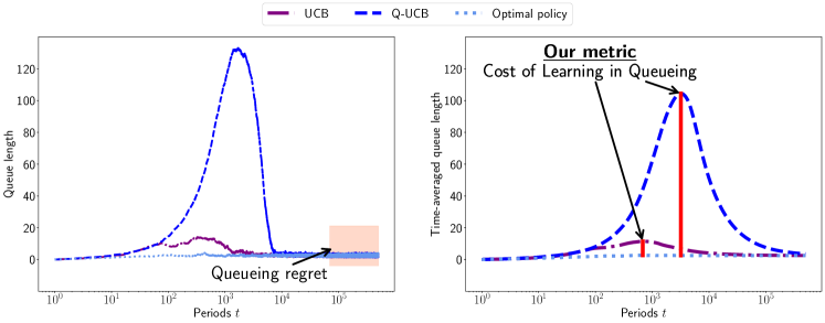
Figure 1: Expected per-period and time-averaged queue lengths of UCB and Q-UCB [KSJS21] in a single-queue setting with $K=5,\lambda=0.45,\boldsymbol{\mu}=(0.045,0.35,0.35,0.35,0.55)$; results are averaged over 50 runs. The difference between both algorithms’ queue lengths is indistinguishable asymptotically (left figure) though they clearly differ in their learning efficiency for early periods as illustrated by Cost of Learning in Queueing, the metric that our work introduces (right figure).

Cost of learning in queueing.

Tackling the first question, we propose the Cost of Learning in Queueing (CLQ) to capture the efficiency of a learning algorithm in queueing systems. The CLQ of a learning policy is defined as the maximum difference of its time-averaged queue length and that of any other policy (with knowledge of parameters) over the entire horizon (see Fig 1 on the right). In contrast to queueing regret, CLQ is 1) a finite-time metric that captures the learning efficiency in early periods and 2) focused on time-averaged queue length instead of per-period queue length. This is favorable as for any periods $1,\ldots,T$, the time-averaged queue length is related to the average wait time by Little’s Law. The formal definition of CLQ can be found in Section 3.

Lower bound of CLQ (Theorem 1).

To characterize the statistical complexity of learning in queueing systems, we consider the simplest non-trivial stabilizable setting that involves one queue and $K$ servers. It is known that the queue length scales as $O(1/\varepsilon)$ under the optimal policy, where $\varepsilon=\mu^{\star}-\lambda$ is the traffic slackness of the system. Fixing $\varepsilon$ and the number of servers $K$, we establish a worst-case lower bound $\Omega(\frac{K}{\varepsilon})$ of CLQ. That is, for any $\varepsilon,K$ and a fixed policy, there always exists a setting of arrival and service rates, such that the CLQ of this policy is at least $\Omega(\frac{K}{\varepsilon})$. Combined with the $O(1/\varepsilon)$ optimal queue length, this lower bound result shows that the effect of learning dominates the performance of queueing systems when $K$ is large (as it may increase the maximum time-averaged queue length by a factor of $K$). This is shown in Figure 1 (right) where the peak of time-averaged queue lengths of the optimal policy with knowledge of parameters is much lower than that of the other two policies (our Algorithm 1 and Q-UCB [KSJS21]).

An efficient algorithm for single-queue multi-server systems (Theorem 2).

Given the above lower bound, we show that the Upper Confidence Bound (UCB) algorithm attains an optimal CLQ up to a logarithmic factor in the single-queue multi-server setting. Our analysis is motivated by Fig. 1 (right) where the time-averaged queue length initially increases and then decreases. Based on this pattern, we divide the horizon into an initial learning stage and a later regenerate stage.

In the learning stage, the time-averaged queue length increases similar to the multi-armed bandit regret. We formalize this observation by coupling the queue under a policy $\pi$ with a nearly-optimal queue and show that their difference is captured by the satisficing regret of policy $\pi$. Satisficing regret resembles the classical multi-armed bandit regret but disregards the loss of choosing a nearly optimal server (see Eq. (8)); this concept is studied from a Bayesian learning perspective in multi-armed bandits [RVR22]. Nevertheless, our result in the learning stage is not sufficient as the satisficing regret eventually goes to infinity.

In the regenerate stage, queue lengths decrease as the policy has learned the parameters sufficiently well; the queue then behaves similarly as under the optimal policy and stabilizes the system. To capture this observation, we use Lyapunov analysis and show that the time-averaged queue length for the initial $T$ periods scales as the optimal queue length, but with an additional term depending on the second moment of satisficing regret divided by $T$. Hence, as $T$ increases, the impact of learning gradually disappears. Combining the results in the learning and regenerate stages, we obtain a tight CLQ bound of UCB for the single-queue multi-server setting.

Efficient algorithms for multi-queue systems and queueing networks (Theorems 3,4).

We next generalize the above result to multi-queue multi-server systems. In contrast to the single queue case, even with known rates, the optimal policy for a multi-queue multi-server system is non-trivial (and usually difficult) to find. A natural greedy policy, such as choosing a set of servers that maximizes instantaneous services as in the single-queue system, is known to have potentially unbounded queue length for a stabilizable system [KAJS18]. Designing an efficient learning policy for multi-queue systems is thus not straightforward.

Instead, we build on the celebrated MaxWeight policy that stabilizes a multi-queue multi-server system with knowledge of system parameters [Tas92]. We design MaxWeight-UCB as a new algorithm to transform MaxWeight into a learning algorithm with appropriate estimates for system parameters and show that its CLQ scales near-optimally as $\tilde{\mathcal{O}}(1/\varepsilon)$ with respect to the traffic slackness $\varepsilon$ (see Definition 2). This dependence greatly improves previous results for settings beyond a single-queue system; the best-known such result is $\tilde{\mathcal{O}}(1/\varepsilon^{3})$ for the special case of a bipartite queueing systems [FLW23, YSY23] (or $\tilde{\mathcal{O}}(1/\varepsilon^{2})$ with additional structural assumptions on service rates [KSJS21]). This result extends our analysis for single-queue settings through a coupling approach that reduces the loss incurred by learning in a high-dimensional queue-length vector to a scalar-valued potential function and builds upon recent work of [Gup22, WXY23].

Finally, we consider queueing networks that include multiple queues, multiple servers, and transitions of served jobs from servers to queues. For this setting, we propose BackPressure-UCB, which incorporates online learning into the BackPressure algorithm [Tas92]. We prove that its CLQ also scales near-optimally as $\tilde{\mathcal{O}}(1/\varepsilon)$. To the best of our knowledge, this is the first efficient learning algorithm for general queueing networks (see related work for a discussion).

Related work.

A recent line of work studies online learning in queueing systems [WX21]. To capture uncertainty in services, [Wal14] studies a single-queue setting in which the DM selects a mode of service in each period and the job service time varies between modes (the dependence is a priori unknown and revealed to the DM after the service). The metric of interest is the queueing regret, i.e., the difference of queue length between an algorithm and the optimal policy, for which the authors show a sublinear bound. [KSJS21] considers the same single-queue multi-server setting as ours and show that a forced exploration algorithm achieves a queueing regret scaling of $\tilde{O}(1/T)$ (under strong structural assumptions this result extends to multiple queues). [SSM21] shows that by probing servers when the queue is idle, it is possible to give an algorithm with queueing regret converging as $O(1/T)$. However, with respect to the traffic slackness $\varepsilon\to 0^{+}$, both bounds yield suboptimal CLQ: [KSJS21] gives at least $O(1/\varepsilon^{2})$ and [SSM21] gives at least $O(1/\varepsilon^{4})$ (see Appendices A.1, A.2). In the analysis of [KSJS21], forced exploration is used for low adaptive regret, i.e., regret over any interval [HS09]; no such guarantee is known for adaptive exploration. But as noted by our Figure 1 and [KSJS21, Figure 2], an adaptive exploration algorithm like UCB has a better early-stage performance than Q-UCB. Using our framework in Section 4, we show that UCB indeed has a near-optimal CLQ that scales as $O(\frac{K}{\varepsilon}\ln\frac{K}{\varepsilon})$. Our framework also allows us to show that Q-UCB enjoys a CLQ scaling as $O(\frac{K}{\varepsilon}\ln\frac{K}{\varepsilon}+\ln^{3}\frac{K}{\varepsilon})$ (Appendix A.1). This improves the guarantee implied by [KSJS21] and shows the inefficiency due to forced exploration is about $O(\ln^{3}\frac{K}{\varepsilon})$ and that Q-UCB has both strong transient (CLQ) and asymptotic (queueing regret) performance.

Focusing on the scaling of queueing regret, [KAJS18] and [ZBW22] study the scheduling in multi-queue settings (with [ZBW22] also considering job abandonment), [CJWS21, FM22] study learning for a load balancing model, [CLH23] studies pricing and capacity sizing for a single-queue single-server model with unknown parameters. For more general settings, [AS23] designs a Bayesian learning algorithm for Markov Decision Processes with countable state spaces (of which queueing systems are special cases) where parameters are sampled from a known prior over a restricted parameter space; in contrast, our paper does not assume any prior of the unknown parameters. The main difference between all of these works and ours is that we focus on how the maximum time-averaged queue lengths scales with respect to system parameters (traffic slackness and number of queues and servers), not on how the queue lengths scale as time grows. Apart from the stochastic learning setting we focus on, there are also works that tackle adversarial learning in queueing systems [HGH23, LM18]; these require substantially different algorithms and analyses.

Going beyond queueing regret, there are papers focusing on finite-time queue length guarantees. In a multi-queue multi-server setting, it is known that the MaxWeight algorithm has a polynomial queue length for stabilizable systems. However, it requires knowledge of system parameters. For a joint scheduling and utility maximization problem, [NRP12] combines MaxWeight with forced exploration to handle parameter uncertainty. By selecting a suitable window for sample collection, their guarantee corresponds to a CLQ bound of at least $O(K^{4}/\varepsilon^{3})$ for our single-queue setting (see Appendix A.3). [SSM19] studies a multi-queue multi-server setting and propose a frame-based learning algorithm based on MaxWeight. They focus on a greedy approximation which has polynomial queue lengths when the system is stabilizable with twice of the arrival rates. [YSY23] considers a non-stationary setting and shows that combining MaxWeight with discounted UCB estimation leads to stability and polynomial queue length that scales as $\tilde{O}(1/\varepsilon^{3})$ (Appendix A.4). There is also a line of work studying decentralized learning in multi-queue multi-server settings. [GT23] assumes queues are selfish and derives conditions under which a no-regret learning algorithm is stable; this is generalized to queueing networks in which queues and servers form a directed acyclic graph by [FHL22]. [SBP21] allows collaborative agents and gives an algorithm with maximum stability, although the queue length scales exponentially in the number of servers. [FLW23] designs a decentralized learning version of MaxWeight and shows that the algorithm always stabilizes the system with polynomial queue lengths $\tilde{O}(1/\varepsilon^{3})$ (Appendix A.5). In contrast to the above, our work shows for the centralized setting that MaxWeight with UCB achieves the near-optimal time-averaged queue length guarantee of $\tilde{O}(1/\varepsilon)$.

Our paper extends the ability of online learning to general single-class queueing networks [BDW21]. The literature considers different complications that arise in these settings, including jobs of different classes and servers that give service simultaneously to different jobs [Tas92, DL05, BDW21]. For the class of networks we consider, it is known that BackPressure can stabilize the system with knowledge of system parameters [Tas92]. Noted in [BDW21], one potential drawback of BackPressure is its need of full knowledge of job transition probabilities. In this regard, our paper contributes to the literature by proposing the first BackPressure-based algorithm that stabilizes queueing networks without knowledge of system parameters.

Moving beyond our focus on uncertainties in services, an orthogonal line of work studies uncertainties in job types. [ADVS13] considers a single server setting where an arriving job belongs to one of two types; but the true type is unknown and is learned by services. They devise a policy that optimizes a linear function of the numbers of correctly identified jobs and the waiting time. [BM19] studies a similar setting with two types of servers where jobs can route from one server to the others. They focus on the impact on stability due to job type uncertainties. [MX18, SGMV20] consider multiple job types and server types. Viewing Bayesian updates as job type transitions, they use queueing networks to model the job learning process and give stable algorithms based on BackPressure. [JKK21, HXLB22] consider online matchings between jobs with unknown payoffs and servers where the goal is to maximize the total payoffs subject to stability. As noted in [MX18, SGMV20, JKK21], one key assumption of this line of work is the perfect knowledge of server types (and job transition probability). Our result for queueing networks thus serves as a step to consider both server uncertainties and job uncertainties, at least in a context without payoffs.

Concurrently to our work, [NM23] proposes a frame-based MaxWeight algorithm with sliding-window UCB for scheduling in a general multi-queue multi-server system with non-stationary service rates. With a suitable frame size (depending on the traffic slackness), they show stability of the algorithm and obtain a queue length bound of $\tilde{O}(1/\varepsilon^{3})$ in the stationary setting (Appendix A.6).

2 Model

We consider a sequential learning setting where a decision maker (DM) repeatedly schedules jobs to a set of servers of unknown quality over discrete time periods $t=1,2,\ldots$. For any $T$, we refer to the initial $T$ periods as the time horizon $T$. To ease exposition, we first describe the simpler setting where there is only one job type (queue) and subsequently extend our approach to a general setting with multiple queues that interact through a network structure.

2.1 Single-queue multi-server system

A single-queue multi-server system is specified by a tuple $(\mathcal{K},\lambda,\boldsymbol{\mu})$. There is one queue of jobs and a set of servers $\mathcal{K}$ with $|\mathcal{K}|=K$. The arrival rate of jobs is $\lambda$, that is, in each period there is a probability $\lambda$ that a new job arrives to the queue. The service rate of a server $k\in\mathcal{K}$, that is, the probability it successfully serves the job it is scheduled to work on, is $\mu_{k}$. Let $Q(t)$ be the number of jobs at the start of period $t$. Initially there is no job and $Q(1)=0$.

Figure 2 summarizes the events that occur in each period $t$. If there is no job in the queue, i.e., $Q(t)=0$, then the DM selects no server; to ease notation, they select the null server $J(t)=\perp$. Otherwise, the DM selects a server $J(t)\in\mathcal{K}$

Figure 2: Flowchart for a single-queue multi-server system.

and requests service for the first job in the queue. The service request is successful with probability $\mu_{J(t)}$ and the job then leaves the system; otherwise, it remains in the queue. At the end of the period, a new job arrives with probability $\lambda$. We assume that arrival and service events are independent. Let $A(t)$ and $\{S_{k}(t)\}_{k\in\mathcal{K}}$ be a set of independent Bernoulli random variables such that $\mathbb{E}\left[A(t)\right]=\lambda$ and $\mathbb{E}\left[S_{k}(t)\right]=\mu_{k}$ for $k\in\mathcal{K}$; for the null server, $\mu_{\perp}=S_{\perp}(t)=0$ for all $t$. The queue length dynamics are thus given by

$$Q(t+1)=Q(t)-S_{J(t)}(t)+A(t).$$ (1)

A non-anticipatory policy $\pi$ for the DM maps for every period $t$ the historical observations until $t$, i.e., $(A(\tau),S_{J(\tau)}(\tau))_{\tau<t}$, to a server $J(t)\in\mathcal{K}\cup\{\perp\}$. We define $Q(t,\pi)$ as the queue length in period $t$ under policy $\pi$. The DM’s goal is to select a non-anticipatory policy $\pi$ such that for any time horizon $T\geq 1$, the expected time-averaged queue length $\frac{1}{T}\sum_{t\leq T}\mathbb{E}\left[Q(t,\pi)\right]$ is as small as possible.

When service rates are known, the policy $\pi^{\star}$ selecting the server with the highest service rate $\mu^{\star}$ in every period (unless the queue is empty) minimizes the expected time-averaged queue length for any time horizon [KSJS21, SSM21]. If $\lambda\geq\mu^{*}$, even under $\pi^{\star}$, the expected time-averaged queue length goes to infinity as the time horizon increases. We thus assume $\lambda<\mu^{\star}$, in which case, the system is stabilizable, i.e., the expected time-averaged queue length under $\pi^{\star}$ is bounded by a constant over the entire time horizon. We next define the traffic slackness of this system:

Definition 1.

A single-queue multi-server system has a traffic slackness $\varepsilon\in(0,1]$ if $\lambda+\varepsilon\leq\mu^{\star}$.

A larger traffic slackness implies that a system is easier to stabilize. It is known that the policy $\pi^{\star}$ obtains an expected time-averaged queue length of the order of $\frac{1}{\varepsilon}$ [SY14].

2.2 Queueing network

A queueing network extends the above case by having multiple queues and probabilistic job transitions after service completion; our model here resembles the one in [BDW21]. A queueing network is defined by a tuple $(\mathcal{N},\mathcal{K},\boldsymbol{\Lambda},\boldsymbol{\mu},\boldsymbol{\mathcal{A}},\boldsymbol{\Sigma},\boldsymbol{\mathcal{B}},\boldsymbol{\mathcal{D}},\bm{P})\$, where $\boldsymbol{\mathcal{B}}=\{\mathcal{B}_{n}\}_{n\in\mathcal{N}}$, $\boldsymbol{\mathcal{D}}=\{\mathcal{D}_{k}\}_{k\in\mathcal{K}}$ and $\bm{P}=(p_{k,n})_{k\in\mathcal{K},n\in\mathcal{N}\cup\{\perp\}}$ such that $\sum_{n\in\mathcal{N}\cup\{\perp\}}p_{k,n}=1,\forall k$. In contrast to the single-queue case, there is now a set of queues $\mathcal{N}$ with cardinality $N$ and a virtual queue $\perp$ to which jobs transition once they leave the system. Each queue $n\in\mathcal{N}$ has a set of servers $\mathcal{B}_{n}$, each of which belongs to a single queue. As before, the service rate of server $k$ is $\mu_{k}$. The set $\mathcal{D}_{k}$ contains the destination queues of server $k$ (and can include the virtual queue $\perp$).

In each period $t$, the DM selects a set of servers to schedule jobs to and, if a service request from queue $n$ to server $k$ is successful, a job from queue $n$ transitions to a queue $n^{\prime}\in\mathcal{D}_{k}$ with probability $p_{k,n^{\prime}}$ (this implies $p_{k,n^{\prime}}=0$ if $n^{\prime}\not\in\mathcal{D}_{k}$). The selected set of servers comes from a set of feasible schedules $\boldsymbol{\Sigma}\subseteq\{0,1\}^{\mathcal{K}}$, which captures interference between servers. We require that for any queue, the number of selected servers is no larger than the number of jobs in this queue. Formally, letting $\sigma_{k}=1$ if schedule $\boldsymbol{\sigma}\in\boldsymbol{\Sigma}$ selects server $k$ and denoting $\boldsymbol{Q}(t)=(Q_{n}(t))_{n\in\mathcal{N}}$ as the queue length vector at the beginning of period $t$, the set of feasible schedules in this period is

$$\boldsymbol{\Sigma}_{t}=\{\boldsymbol{\sigma}\in\boldsymbol{\Sigma}\colon\sum_{k\in\mathcal{B}_{n}}\sigma_{k}\leq Q_{n}(t),\forall n\in\mathcal{N}\}$$ (2)

and the DM’s decision in period $t$ is to select a schedule $\boldsymbol{\sigma}(t)\in\boldsymbol{\Sigma}_{t}$. Following [Tas92], we assume that any subset of a feasible schedule is still feasible, i.e., if $\boldsymbol{\sigma}\in\boldsymbol{\Sigma}$ and $\sigma^{\prime}_{k}\leq\sigma_{k}~{}\forall k\in\mathcal{K}$, then $\boldsymbol{\sigma}^{\prime}\in\boldsymbol{\Sigma}$.

We now illustrate how this formulation captures interesting special cases (see Appendix B for further details). The single-queue multi-server system considered above assumes a single queue ($N=1$), no job transitions ($\mathcal{D}_{k}=\{\perp\}$), and a DM that selects at most one server every period, i.e., $\boldsymbol{\Sigma}=\{\emptyset,\{k\}_{k\in\mathcal{K}}\}$. The bipartite queueing system in [FLW23] allows for the selection of a bipartite matching between $N$ queues and $M$ workers in every period. This can be captured as a queueing network with no job transitions by setting the set of servers $\mathcal{K}$ as the set of all queue-worker pairs and letting $\boldsymbol{\Sigma}$ be the set of all possible matchings. The multi-server system in [YSY23] extends this setting by allowing a queue to be matched to multiple workers, i.e., $\boldsymbol{\Sigma}$ includes all subsets of pairs where each worker is matched to at most one queue. Motivated by crowdsourcing, the expert learning system in [SGMV20] further extends this setting by allowing servers to refine uncertainties in job types. Arriving jobs come with a known prior distribution for their types and this distribution is gradually learned by workers’ services. This model can be captured by a queueing network such that the set of queues $\mathcal{N}$ corresponds to all type distributions and $p_{k,n}$ is the probability that a job served by server $k$ has posterior type distribution $n$. [SGMV20] assumes full knowledge of transition probabilities and service rates and states tackling uncertainties in these quantities as a future direction. Our work tackles these uncertainties when the set $\mathcal{N}$ is finite ([SGMV20] allows for countably many queues).

We now formalize the arrival and service dynamics in every period, which are captured by the independent random variables $\{\boldsymbol{A}(t),\{S_{k}(t)\}_{k\in\mathcal{K}}\}_{t}$. The arrival vector $\boldsymbol{A}(t)=\{A_{n}(t)\}_{n\in\mathcal{N}}$ consists of (possibly correlated) random variables $A_{n}(t)$ taking value in $\boldsymbol{\mathcal{A}}\subseteq\{0,1\}^{\mathcal{N}}$; we denote its distribution by $\boldsymbol{\Lambda}$ and let $\mathbb{E}\left[A_{n}(t)\right]=\lambda_{n}(\boldsymbol{\Lambda})$ with $\boldsymbol{\lambda}=(\lambda_{n}(\boldsymbol{\Lambda}))_{n\in\mathcal{N}}$. The service $S_{k}(t)$ for each server $k\in\mathcal{K}$ is a Bernoulli random variable indicating whether the selected service request was successful. To formalize the job transition, let $\boldsymbol{L}_{k}(t)=(L_{k,n}(t))_{n\in\mathcal{N}\cup\{\perp\}}$ be a random vector over $\{0,1\}^{\mathcal{N}\cup\{\perp\}}$ for server $k$ independent of other randomness such that $\mathbb{P}\{L_{k,n}(t)=1\}=p_{k,n}$ and $\sum_{n\in\mathcal{N}\cup\{\perp\}}L_{k,n}(t)=1$. The queueing dynamic is given by

$$Q_{n}(t+1)=Q_{n}(t)-\sum_{k\in\mathcal{B}_{n}}\sigma_{k}(t)S_{k}(t)+A_{n}(t)+\sum_{k^{\prime}\in\mathcal{K}}\sigma_{k^{\prime}}(t)S_{k^{\prime}}(t)L_{k^{\prime},n}(t).$$ (3)

We assume that the DM has knowledge of which policies are allowed, i.e., they know $\boldsymbol{\Sigma}$ and $\boldsymbol{\mathcal{B}}$, but has no prior knowledge of the rates $\boldsymbol{\lambda},\boldsymbol{\mu},\bm{P}$ and the set $\boldsymbol{\mathcal{D}}$ . In period $t$, the observed history is the set $\left(\{A_{n}(\tau)\}_{n\in\mathcal{N}},\{S_{k}(\tau)L_{k,n}(\tau)\}_{n\in\bar{\mathcal{N}},k\in\mathcal{K}\colon\sigma_{k}(\tau)=1}\right)_{\tau<t}$ that includes transition information on top of arrivals and services. Note that a job transition is only observed when the server is selected and the service is successful. Similar to before, a non-anticipatory policy $\pi$ maps an observed history to a feasible schedule; we let $Q_{n}(t,\pi)$ be the length of queue $n$ in period $t$ under this policy.

Unlike the single-queue case, it is usually difficult to find the optimal policy for a queueing network even with known system parameters. Fortunately, if the system is stabilizable, i.e., $\lim_{t\to\infty}\frac{1}{T}\sum_{t\leq T}\mathbb{E}\left[\|\boldsymbol{Q}(t)\|_{1}\right]<\infty$ under some scheduling policy, then the arrival rate vector must be within the capacity region of the servers [Tas92]. Formally, let $\boldsymbol{\Phi}=\{\boldsymbol{\phi}\in[0,1]^{\boldsymbol{\Sigma}}\colon\sum_{\boldsymbol{\sigma}\in\boldsymbol{\Sigma}}\boldsymbol{\phi}_{\boldsymbol{\sigma}}=1\}$ be the probability simplex over $\boldsymbol{\Sigma}$. A distribution $\boldsymbol{\phi}$ in $\boldsymbol{\Phi}$ can be viewed as the frequency of a policy using each schedule $\boldsymbol{\sigma}\in\boldsymbol{\Sigma}$, and the effective service rate queue $n$ can get is given by $\mu_{n}^{\mathrm{net}}(\boldsymbol{\phi})=\sum_{\boldsymbol{\sigma}\in\boldsymbol{\Sigma}}\boldsymbol{\phi}_{\boldsymbol{\sigma}}\left(\sum_{k\in\mathcal{B}_{n}}\sigma_{k}\mu_{k}-\sum_{k^{\prime}\in\mathcal{K}}\sigma_{k^{\prime}}\mu_{k^{\prime}}p_{k^{\prime},n}\right)$; this includes both job inflow and outflow. We denote the effective service rate vector for a schedule distribution $\boldsymbol{\phi}$ by $\boldsymbol{\mu}^{\mathrm{net}}(\boldsymbol{\phi})$. Then, the capacity region is $\mathcal{S}(\boldsymbol{\mu},\boldsymbol{\Sigma},\boldsymbol{\mathcal{B}},\bm{P})=\{\boldsymbol{\mu}^{\mathrm{net}}(\boldsymbol{\phi})\colon\boldsymbol{\phi}\in\boldsymbol{\Phi}\}$. For a queueing network to be stabilizable, we must have $\boldsymbol{\lambda}(\boldsymbol{\Lambda})\in\mathcal{S}(\boldsymbol{\mu},\boldsymbol{\Sigma},\boldsymbol{\mathcal{B}},\bm{P})$ [Tas92]. As in the single-queue case, we further assume that the system has a positive traffic slackness and let $\bm{1}$ denote a vector of $1$s with suitable dimension.

Definition 2.

A queueing network has traffic slackness $\varepsilon\in(0,1]$ if $\boldsymbol{\lambda}(\boldsymbol{\Lambda})+\varepsilon\bm{1}\in\mathcal{S}(\boldsymbol{\mu},\boldsymbol{\Sigma},\boldsymbol{\mathcal{B}},\bm{P})$.

We also study a special case of queueing networks, multi-queue multi-server systems, where jobs immediately leave after a successful service, i.e., $\mathcal{D}_{k}=\{\perp\}$ for all $k\in\mathcal{K}$; this extends the models in [FLW23, YSY23] mentioned above. Since the transition probability matrix $\bm{P}$ is trivial ($p_{k,\perp}=1,\forall k$), we denote the capacity region of a multi-queue multi-server system by $\mathcal{S}(\boldsymbol{\mu},\boldsymbol{\Sigma},\boldsymbol{\mathcal{B}})$.

3 Main results: the statistical complexity of learning in queueing

This section presents our main results on the statistical complexity of learning in queueing systems. We first define the Cost of Learning in Queueing, or CLQ as a shorthand, a metric capturing this complexity and provide a lower bound for the single-queue multi-server setting. Motivated by this, we design an efficient algorithm for the single-queue multi-server setting with a matching CLQ and then extend this to the multi-queue multi-server and queueing network systems.

3.1 Cost of Learning in Queueing

We first consider learning in the single-queue multi-server setting. Previous works on learning in queueing systems focus on the queueing regret $\mathbb{E}\left[Q(T,\pi)-Q(T,\pi^{\star})\right]$ in the asymptotic regime of $T\to\infty$. The starting point of our work stems from the observation that an asymptotic metric, which measures performance in late periods, cannot capture the complexity of learning as learning happens in initial periods (recall the left of Figure 1). In addition, a guarantee on per-period queue length cannot easily translate to the service experience (or wait time) of jobs.

Motivated by the above insufficiency of queueing regret, we define the Cost of Learning in Queueing (or CLQ) as the maximum increase in expected time-averaged queue lengths under policy $\pi$ compared with the optimal policy. Specifically, we define the single-queue CLQ  as:

$$\textsc{CLQ}^{\mathrm{single}}(\lambda,\boldsymbol{\mu},\pi)=\max_{T\geq 1}\frac{\sum_{t=1}^{T}\mathbb{E}\left[Q(t,\pi)-Q(t,\pi^{\star})\right]}{T}.$$ (4)

As shown in Figure 1 (right), CLQ  is a finite-time metric and explicitly takes into account how fast learning occurs in the initial periods. In addition, a bound on the maximum increase in time-averaged queue length translates approximately (via Little’s Law [Lit61]) to a bound on the increase in average job wait times.

Given that the traffic slackness measures the difficulty of stabilizing a system, we also consider the worst-case cost of learning in queueing over all pairs of $(\lambda,\boldsymbol{\mu})$ with a fixed traffic slackness $\varepsilon$. In a slight abuse of notation, we overload $\textsc{CLQ}^{\mathrm{single}}$ to also denote this worst-case value, i.e.,

$$\textsc{CLQ}^{\mathrm{single}}(K,\varepsilon,\pi)=\sup_{\lambda\in[0,1),\boldsymbol{\mu}\in[0,1]^{K}\colon\lambda+\varepsilon\leq\max_{k}\mu_{k}}\textsc{CLQ}^{\mathrm{single}}(\lambda,\boldsymbol{\mu},\pi).$$ (5)

Our goal is to design a policy $\pi$, without knowledge of the arrival rate, the service rates, and the traffic slackness, that achieves low worst-case cost of learning in a single-queue multi-server system.

We can extend the definition of CLQ to the multi-queue multi-server and the queueing network settings. Since the optimal policy is difficult to design, we instead define CLQ for a policy $\pi$ by comparing it with any non-anticipatory policy (which makes decisions only based on the history):

$$\textsc{CLQ}^{\mathrm{multi}}(\boldsymbol{\Lambda},\boldsymbol{\mu},\boldsymbol{\Sigma},\boldsymbol{\mathcal{B}},\pi)=\max_{\text{non-anticipatory }\pi^{\prime}}\max_{T\geq 1}\frac{\sum_{t=1}^{T}\sum_{n\in\mathcal{N}}\mathbb{E}\left[Q_{n}(t,\pi)-Q_{n}(t,\pi^{\prime})\right]}{T}.$$ (6)

$$\textsc{CLQ}^{\mathrm{net}}(\boldsymbol{\Lambda},\boldsymbol{\mu},\boldsymbol{\Sigma},\boldsymbol{\mathcal{B}},\boldsymbol{\mathcal{D}},\bm{P},\pi)=\max_{\text{non-anticipatory }\pi^{\prime}}\max_{T\geq 1}\frac{\sum_{t=1}^{T}\sum_{n\in\mathcal{N}}\mathbb{E}\left[Q_{n}(t,\pi)-Q_{n}(t,\pi^{\prime})\right]}{T}$$ (7)

As in the single-queue setting, we can define the worst-case cost of learning for a fixed structure $\boldsymbol{\mathcal{A}},\boldsymbol{\Sigma},\boldsymbol{\mathcal{B}},\boldsymbol{\mathcal{D}}$ and a traffic slackness $\varepsilon$ as the supremum across all arrival, service, and transition rates with this traffic slackness. With the same slight abuse of notation as before, we denote these quantities by $\textsc{CLQ}^{\mathrm{multi}}(\boldsymbol{\mathcal{A}},\boldsymbol{\Sigma},\boldsymbol{\mathcal{B}},\varepsilon,\pi)$ and $\textsc{CLQ}^{\mathrm{net}}(\boldsymbol{\mathcal{A}},\boldsymbol{\Sigma},\boldsymbol{\mathcal{B}},\boldsymbol{\mathcal{D}},\varepsilon,\pi)$.

3.2 Lower bound on the cost of learning in queueing

Our first result establishes a lower bound on $\textsc{CLQ}^{\mathrm{single}}(K,\varepsilon,\pi)$. In particular, for any feasible policy $\pi$, we show a lower bound of $\Omega(\frac{K}{\varepsilon})$ for sufficiently large $K$. With known parameters, the optimal time-averaged queue length is of the order of $\nicefrac{{1}}{{\varepsilon}}$. Hence, our result shows that the cost of learning is non-negligible in queueing systems when there are many servers. For fixed $K$ and $\varepsilon$, our lower bound considers the cost of learning of the worst-case setting and is instance-independent.

Theorem 1.

For any $K\geq 2^{14},\varepsilon\in(0,0.25]$ and feasible policy $\pi$, we have $\textsc{CLQ}^{\mathrm{single}}(K,\varepsilon,\pi)\geq\frac{K}{2^{14}\varepsilon}$.

Although our proof is based on the distribution-free lower bound $\Omega(\sqrt{KT})$ for classical multi-armed bandits [ACFS02], this result does not apply directly to our setting. In particular, suppose the queue in our system is never empty. Then the accumulated loss in service of a policy is exactly the regret in bandits and the lower bound implies that any feasible policy serves at least $\Omega(\sqrt{KT})$ jobs fewer than the optimal policy in the first $T$ periods. However, due to the traffic slackness, the queue does get empty under the optimal policy, and in periods when this occurs, the optimal policy also does not receive service. As a result, the queue length of a learning policy could be lower than $\Theta(\sqrt{KT})$ despite the loss of service compared with the optimal policy.

We next discuss the intuition of our proof (formal proof in Appendix C.1). Fixing $K$ and $\varepsilon$, suppose the gap in service rates between the optimal server and others is $2\varepsilon$. Then for any $t$ in a time horizon $T=O(\frac{K}{\varepsilon^{2}})$, the number of arrivals in the first $t$ periods is around $\lambda t$ and the potential service of the optimal server is around $(\lambda+\varepsilon)t$. By the multi-armed bandit lower bound, the total service of a feasible policy is at most around $\lambda t+\varepsilon t-\sqrt{Kt}\leq\lambda t$ since $t\leq T=O(\frac{K}{\varepsilon^{2}})$. Therefore, the combined service rate of servers chosen in the first $T$ periods, i.e., $\sum_{t\leq T}\mu_{J(t)}$, is strictly bounded from above by the total arrival rate $\lambda t$. A carefully constructed example shows that the number of unserved jobs is around $\varepsilon t$ for every $t\leq T$. As a result, the time-averaged queue length for the horizon $T$ is of the order of $\varepsilon T=O(\frac{K}{\varepsilon})$.

Remark 1.

In [KSJS21, Proposition 3], the authors established an instance-dependent lower bound on $\mathbb{E}\left[Q(t,\pi)-Q^{\star}(t)\right]$. The implied CLQ lower bound is weaker than ours ($\tilde{\Omega}(K)$, see Appendix C.2) and is constrained to $\alpha-$consistent policy $\pi$ (see definition 1 in [KSJS21]) whereas ours does not.

3.3 Upper bound on the cost of learning in queueing

Motivated by the lower bound, we propose efficient algorithms with a focus on heavy-traffic optimality, i.e., ensuring $\textsc{CLQ}=\tilde{O}(\nicefrac{{1}}{{\varepsilon}})$ as $\varepsilon\to 0^{+}$. The rationale is that stabilizing the system with unknown parameters is more difficult when the traffic slackness is lower as an efficient algorithm must strive to learn parameters more accurately. We establish below that the classical upper confidence bound policy (UCB, see Algorithm 1) achieves near-optimal $\textsc{CLQ}=\tilde{O}(\frac{K}{\varepsilon})$ for any $K$ and $\varepsilon$ in the single-queue multi-server setting with no prior information of any system parameters.

Theorem 2.

For any $K\geq 1,\varepsilon\in(0,1]$, $\textsc{CLQ}^{\mathrm{single}}(K,\varepsilon,\textsc{UCB})\leq\frac{323K+64K(\ln K+2\ln\nicefrac{{1}}{{\varepsilon}})}{\varepsilon}.$

The proof of the theorem (Section 4) bridges Lyapunov and bandit analysis, makes an interesting connection to satisficing regret, and is a main technical contribution of our work.

We next extend our approach to the queueing network setting. Fixing the system structure $\boldsymbol{\mathcal{A}},\boldsymbol{\Sigma},\boldsymbol{\mathcal{B}},\boldsymbol{\mathcal{D}}$, we define $M_{\boldsymbol{\mathcal{A}}}=\max_{\boldsymbol{A}\in\boldsymbol{\mathcal{A}}}\sum_{n\in\mathcal{N}}A_{n}$ and $M_{\boldsymbol{\Sigma},\boldsymbol{\mathcal{B}}}=\max_{\boldsymbol{\sigma}\in\boldsymbol{\Sigma}}\sum_{n\in\mathcal{N}}\sum_{k\in\mathcal{B}_{n}}\sigma_{k}$, to be the maximum number of new job arrivals and the maximum number of selected servers per period. Further, for queueing networks, we also define the quantity $M_{\boldsymbol{\mathcal{D}}}=\sum_{k\in\mathcal{K}}|\mathcal{D}_{k}|^{2}$, related to the number of queues each server may see its jobs transition to. The following result shows that the worst-case cost of learning of our algorithm BackPressure-UCB (BP-UCB as a short-hand, Algorithm 3 in Section 6) has optimal dependence on $\frac{1}{\varepsilon}$. The proof of this Theorem is provided in Section 6.

Theorem 3.

For any $\boldsymbol{\mathcal{A}},\boldsymbol{\Sigma},\boldsymbol{\mathcal{B}},\boldsymbol{\mathcal{D}}$ and traffic slackness $\varepsilon\in(0,1]$, we have

$$\textsc{CLQ}^{\mathrm{net}}(\boldsymbol{\mathcal{A}},\boldsymbol{\Sigma},\boldsymbol{\mathcal{B}},\boldsymbol{\mathcal{D}},\varepsilon,\textsc{BP-UCB})\leq\frac{\sqrt{N}\left(32M_{\boldsymbol{\mathcal{A}}}+2^{12}M_{\boldsymbol{\mathcal{D}}}M_{\boldsymbol{\Sigma},\boldsymbol{\mathcal{B}}}^{2}\left(1+\ln(M_{\boldsymbol{\mathcal{A}}}M_{\boldsymbol{\mathcal{D}}}M_{\boldsymbol{\Sigma},\boldsymbol{\mathcal{B}}}/\varepsilon)\right)\right)}{\varepsilon}.$$

Our proof builds on the special case of multi-queue multi-server systems, for which we provide Algorithm MaxWeight-UCB with a corresponding performance guarantee (see Section 5).

4 Optimal cost of learning for single-queue multi-server systems

In this section, we bound the CLQ of UCB for the single-queue multi-server setting (Theorem 2). In each period $t$, when the queue is non-empty, UCB selects a server with the highest upper confidence bound estimation $\bar{\mu}_{k}(t)=\min\left(1,\hat{\mu}_{k}(t)+\sqrt{\frac{2\ln(t)}{C_{k}(t)}}\right)$ where $\hat{\mu}_{k}(t)$ is the sample mean of services and $C_{k}(t)$ is the number of times server $k$ is selected in the first $t-1$ periods.

1 Sample mean $\hat{\mu}_{k}(1)\leftarrow 0$, number of samples $C_{k}(1)\leftarrow 0$ for $k\in\mathcal{K}\cup\{\perp\}$, queue $Q(1)\leftarrow 0$

for $t=1\ldots$ do

      2 $\bar{\mu}_{k}(t)=\min\left(1,\hat{\mu}_{k}(t)+\sqrt{\frac{2\ln(t)}{C_{k}(t)}}\right),\forall k\in\mathcal{K}$

      3 if $Q(t)>0$ then $J(t)\leftarrow\arg\max_{k}\bar{\mu}_{k}(t)$

      4 else $J(t)\leftarrow\perp$

       /* Update queue length & estimates based on $S_{J(t)}(t)$, $A(t)$, and $J(t)$ */

5       $Q(t+1)\leftarrow Q(t)-S_{J(t)}(t)+A(t)$

6       $C_{J(t)}(t+1)\leftarrow C_{J(t)}(t)+1,\quad\hat{\mu}_{J(t)}(t+1)\leftarrow\frac{C_{J(t)}(t)\hat{\mu}_{J(t)}(t)+S_{J(t)}(t)}{C_{J(t)}(t+1)}$

7       for $k\neq J(t)$ set $C_{k}(t+1)\leftarrow C_{k}(t),\quad\hat{\mu}_{k}(t+1)\leftarrow\hat{\mu}_{k}(t)$

Algorithm 1 UCB for a single-queue multi-server system

To prove Theorem 2, we establish an analytical framework to upper bound $\textsc{CLQ}^{\mathrm{single}}$ for any policy $\pi$ by considering separately the initial learning stage and the later regenerate stage. The two stages are separated by a parameter $T_{1}$ that appears in our analysis: intuitively, during the learning stage ($t<T_{1}$), the loss in total service of a policy compared with the optimal server’s outweighs the slackness $\varepsilon$ of the system (Definition 1), i.e., $\sum_{\tau=1}^{t}\mu^{\star}-\mu_{J(\tau)}>t\varepsilon$ and thus the queue length grows linearly with respect to the left-hand side. After the learning stage ($t>T_{1}$), when $\sum_{\tau=1}^{t}\mu^{\star}-\mu_{J(\tau)}<t\varepsilon$, the queue regenerates to a constant length independent of $t$. To prove the $\tilde{O}(\frac{K}{\varepsilon})$ bound on $\textsc{CLQ}^{\mathrm{single}}$, we first couple the queue with an “auxiliary” queue where the DM always chooses a nearly optimal server in the learning stage. Then we utilize a Lyapunov analysis to bound the queue length during the regenerate stage.

The framework establishes a connection between $\textsc{CLQ}^{\mathrm{single}}(\lambda,\boldsymbol{\mu},\pi)$ and the satisficing regret defined as follows. For any horizon $T$, the satisficing regret $\mathrm{SaR}^{\mathrm{single}}(\pi,T)$ is the total service rate gap between the optimal server and the server selected by $\pi$ except for the periods where the gap is less than $\frac{\varepsilon}{2}$ or the queue length is zero. That is, the selected server is satisficing as long as its service rate is nearly optimal or the queue is empty. To formally define it, we denote $\max(x,0)$ by $x^{+}$ and define the satisficing regret of a policy $\pi$ over the first $T$ periods by

$$\mathrm{SaR}^{\mathrm{single}}(\pi,T)=\sum_{t=1}^{T}\left(\mu^{\star}-\mu_{J(t)}-\frac{\varepsilon}{2}\right)^{+}\mathbbm{1}\left(Q(t)\geq 1\right)$$ (8)

We use the satisficing regret terminology because our motivation for $\mathrm{SaR}^{\mathrm{single}}(\pi,T)$ is similar to that in multi-armed bandits [RVR22], initially considered for an infinite horizon and a Bayesian setting. In multi-armed bandits, optimal bounds on regret $\sum_{t=1}^{T}(\mu^{\star}-\mu_{J(t)})$ are either instance-dependent $\mathcal{O}\left(\sum_{k\colon\mu_{k}<\mu^{\star}}\left(\frac{1}{\mu^{\star}-\mu_{k}}\ln T\right)\right)$ [ACF02] or instance-independent $O(\sqrt{KT})$ [ACFS02]. However, both are futile to establish a $\tilde{\mathcal{O}}(\frac{K}{\varepsilon})$ bound for $\textsc{CLQ}^{\mathrm{single}}(K,\varepsilon)$: The first bound depends on the minimum gap (which can be infinitesimal), whereas the second is insufficient as we explain in the discussion after Lemma 4.2.

We circumvent these obstacles by connecting the time-averaged queue length of the system with the satisficing regret of the policy via Lemma 4.1 (for the learning stage) and Lemma 4.2 (for the regenerate stage). Lemma 4.1 explicitly bounds the expected queue length through the expected satisficing regret; this is useful during the learning stage but does not give a strong bound for the regenerate stage. Lemma 4.2 gives a bound that depends on $\frac{\mathrm{SaR}^{\mathrm{single}}(\pi,T)^{2}}{T}$, and is particularly useful during the latter regenerate stage. We then show that the satisficing regret of UCB is $O(\frac{K\ln T}{\varepsilon})$ (Lemma 4.3). Combining these results, we establish a tight bound for the cost of learning of UCB.

Formally, Lemma 4.1 shows that the expected queue length under $\pi$ in period $t$ is at most that under a nearly optimal policy plus the expected satisficing regret up to that time.

Lemma 4.1.

For any policy $\pi$ and horizon $T$, we have $\frac{\sum_{t=1}^{T}\mathbb{E}\left[Q(t)\right]}{T}\leq\frac{3}{\varepsilon}+\mathbb{E}\left[\mathrm{SaR}^{\mathrm{single}}(\pi,T)\right]$.

Lemma 4.1 is established by coupling the queue with an auxiliary queue that always selects a nearly optimal server. However, it cannot provide a useful bound on the cost of learning. For large $T$, it is known that $\mathbb{E}\left[\mathrm{SaR}^{\mathrm{single}}(\pi,T)\right]$ must grow with a rate of at least $\mathcal{O}(\frac{\log T}{\varepsilon})$ [LR85]. Hence, Lemma 4.1 only meaningfully bounds the queue length for small $T$ (learning stage). For large $T$ (regenerate stage), we instead have the following bound (Lemma 4.2).

Lemma 4.2.

For any policy $\pi$ and horizon $T$, we have $\frac{\sum_{t=1}^{T}\mathbb{E}\left[Q(t)\right]}{T}\leq\frac{4}{\varepsilon}+\frac{8}{\varepsilon^{2}}\cdot\frac{\mathbb{E}\left[\mathrm{SaR}^{\mathrm{single}}(\pi,T)^{2}\right]}{T}$.

This lemma shows that the impact of learning, reflected by $\mathbb{E}\left[\mathrm{SaR}^{\mathrm{single}}(\pi,T)^{2}\right]$, decays at a rate of $\frac{1}{T}$. Therefore, as long as $\mathrm{SaR}^{\mathrm{single}}(\pi,T)^{2}$ is of a smaller order than $T$, the impact of learning eventually disappears. This also explains why the instance-independent $O(\sqrt{KT})$ regret bound for multi-armed bandits is insufficient for our analysis: the second moment of the regret scales linearly with the horizon and does not allow us to show a decreasing impact of learning on queue lengths.

Lemma 4.2 suffices to show stability ($\lim_{T\to\infty}\frac{\sum_{t=1}^{T}\mathbb{E}\left[Q(t)\right]}{T}<\infty$), but gives a suboptimal bound for small $T$. Specifically, when $\mathrm{SaR}^{\mathrm{single}}(\pi,T)^{2}\gtrapprox T$, this bound is of the order of $\Omega(\frac{1}{\varepsilon^{2}})$. We thus need both Lemma 4.1 and Lemma 4.2 to establish a tight bound on the cost of learning in queues.

The following result bounds the first and second moments of the satisficing regret of UCB.

Lemma 4.3.

For any horizon $T$, we have

$$(i)\quad\mathbb{E}\left[\mathrm{SaR}^{\mathrm{single}}(\textsc{UCB},T)\right]\leq\frac{16K(\ln T+2)}{\varepsilon},~{}\quad(ii)\quad\mathbb{E}\left[\mathrm{SaR}^{\mathrm{single}}(\textsc{UCB},T)^{2}\right]\leq\frac{2^{9}K^{2}(\ln T+2)^{2}}{\varepsilon^{2}}.$$

Proof of Theorem 2.

Fix $K,\varepsilon$ and any pair of $\lambda,\boldsymbol{\mu}=(\mu_{1},\ldots,\mu_{K})$ such that $\max_{k\in\mathcal{K}}\mu_{k}=\lambda+\varepsilon$. Let $T_{1}=\left\lfloor\left(\frac{2^{12}K^{2}}{\varepsilon^{4}}\right)^{2}\right\rfloor$. We establish an upper bound on $\textsc{CLQ}^{\mathrm{single}}(\lambda,\boldsymbol{\mu},\textsc{UCB})$ by bounding the time-averaged queue length for $T\leq T_{1}$ (learning stage) and $T\geq T_{1}$ (regenerate stage) separately.

For $T\leq T_{1}$, we have

$$\frac{1}{T}\sum_{t\leq T}\mathbb{E}\left[Q(t)\right] \leq\frac{3}{\varepsilon}+\mathbb{E}\left[\mathrm{SaR}^{\mathrm{single}}(\textsc{UCB},T)\right]$$ (Lemma 4.1)

$$\leq\frac{3}{\varepsilon}+\frac{16K(\ln T_{1}+2)}{\varepsilon} T\leq T_{1}$$ (Lemma 4.3 (i) and )

$$\leq\frac{3+32K}{\varepsilon}+\frac{32K\ln\left(\nicefrac{{2^{12}K^{2}}}{{\varepsilon^{4}}}\right)}{\varepsilon} T_{1}\leq\left(\frac{2^{12}K^{2}}{\varepsilon^{4}}\right)^{2}$$ ( by definition)

$$\leq\frac{323K+64K(\ln K+2\ln\nicefrac{{1}}{{\varepsilon}})}{\varepsilon}.$$

For $T>T_{1}$, we have

$$\frac{1}{T}\sum_{t\leq T}\mathbb{E}\left[Q(t)\right] \leq\frac{4}{\varepsilon}+\frac{8}{\varepsilon^{2}}\frac{\mathbb{E}\left[\mathrm{SaR}^{\mathrm{single}}(\textsc{UCB},T)^{2}\right]}{T}$$ (Lemma 4.2)

$$\leq\frac{4}{\varepsilon}+\frac{2^{12}K^{2}(\ln T+2)^{2}}{\varepsilon^{4}T}$$ (Lemma 4.3 (ii))

$$\leq\frac{4}{\varepsilon}+\frac{2^{12}K^{2}}{\varepsilon^{4}\sqrt{T}} T\geq T_{1}\geq 50000$$ (Fact 5 (i) and )

$$\leq\frac{5}{\varepsilon}\qquad\leq\frac{323K+64K(\ln K+2\ln\nicefrac{{1}}{{\varepsilon}})}{\varepsilon}.$$ (9)

Combining these cases we bound $\textsc{CLQ}^{\mathrm{single}}(K,\varepsilon,\textsc{UCB})$ by noting that, for any pair of $\lambda,\boldsymbol{\mu}$ with $\max_{k\in\mathcal{K}}\mu_{k}=\lambda+\varepsilon$, $\textsc{CLQ}^{\mathrm{single}}(\lambda,\boldsymbol{\mu},\textsc{UCB})\leq\max_{T}\frac{1}{T}\sum_{t\leq T}\mathbb{E}\left[Q(t)\right]\leq\textsc{CLQ}^{\mathrm{single}}(K,\varepsilon,\textsc{UCB})$. ∎

Remark 2.

Although the CLQ metric is focused on the entire horizon, our analysis extends to bounding the maximum expected time-averaged queue lengths in the later horizon, which is formalized as $\max_{T\geq T_{1}}\frac{\sum_{t\leq T}\mathbb{E}\left[Q(t)\right]}{T}$ for any $T_{1}$. In particular, for $T_{1}\geq\left(\frac{2^{12}K^{2}}{\varepsilon^{4}}\right)^{2}$, (9) shows that $\max_{T\geq T_{1}}\frac{\sum_{t\leq T}\mathbb{E}\left[Q(t)\right]}{T}\leq\frac{5}{\varepsilon}$; UCB thus enjoys the optimal asymptotic queue length scaling of $O(\frac{1}{\varepsilon})$.

4.1 Queue length bound in the learning stage (Lemma 4.1)

To upper bound the queue length during the learning stage (Lemma 4.1), we couple the queue operated under a policy $\pi$ with a queue that is operated near optimally. Intuitively, the difference in queue lengths between two queues is upper bounded by the difference in their total services. In particular, consider a fictitious single-queue single-server system $\{\hat{Q}(t)\}$ that has the same arrival realization of the current process $\{Q(t)\}$ but with one server whose service rate is $\mu^{\star}-\frac{\varepsilon}{2}$. Denote the realization of services by $\hat{S}(t)$. The server in this fictitious system is slightly less efficient than the optimal server in the original system. The reason to couple with such a worse-performing system is twofold: 1) its queue length is still of the order $O(\frac{1}{\varepsilon})$ and 2) the difference in services between the original system and this system is captured by the satisficing regret $\mathrm{SaR}^{\mathrm{single}}(\pi,T)$ (8). That is, when the chosen server under $\pi$ is nearly optimal (larger than $\mu^{\star}-\frac{\varepsilon}{2}$), we do not count the difference in service for this period at all. Such a shift of benchmark from the optimal $\mu^{\star}$ to $\mu^{\star}-\frac{\varepsilon}{2}$ is essential for our analysis to avoid a dependence of the minimal gap between servers’ service rates and the optimal rate (which must exist if one uses the optimal service rate as benchmark as in multi-armed bandits [LR85]). A final piece of the proof is to couple the service process of $\{Q(t)\}$ and $\{\tilde{Q}(t)\}$ (recall that their arrival process is the same), which we show below.

Proof of Lemma 4.1.

Let $\{U(t)\}_{t\geq 1}$ be a sequence of independent random variables of uniform distribution over $[0,1]$. Then we generate $S_{k}(t)$ by setting $S_{k}(t)=\mathbbm{1}\left(U(t)\leq\mu_{k}\right)$; similarly $\tilde{S}(t)=\mathbbm{1}\left(U(t)\leq\mu^{\star}-\frac{\varepsilon}{2}\right)$. Initially $\tilde{Q}(1)=0$. Although this coupling introduces dependency between $\{S_{k}(t)\}_{k\in\mathcal{K}}$ in a period $t$, it does not affect the distribution of the queue length process since in each period the DM selects at most one server (see the argument in EC. 1.1 of [KSJS21]).

The dynamic of $\{\tilde{Q}(t)\}$ is given by $\tilde{Q}(t+1)=(\tilde{Q}(t)-\tilde{S}(t))^{+}+A(t)$. Then by the dynamic of $\{Q(t)\}$ in (1), the difference between the two queues for every period $t>1$ is

$$Q(t+1)-\tilde{Q}(t+1) =Q(t)-S_{J(t)}(t)+A(t)-\left(\tilde{Q}(t)-\tilde{S}(t)+A(t)+\mathbbm{1}\left(\tilde{Q}(t)-\tilde{S}(t)=-1\right)\right)$$

$$\leq\left(Q(t)-\tilde{Q}(t)+\tilde{S}(t)-S_{J(t)}(t)\right)\mathbbm{1}\left(Q(t)\geq 1\right),$$ (10)

where the inequality is because we have $Q(t+1)\geq A(t)=Q(t)$ when $Q(t)=0$. For any fixed period $t$, define $\mathrm{Emp}(t)=\max\{\tau<t\colon Q(\tau)=0\}$ as the latest period before $t$ such that the queue length is zero. Applying (10) recursively from $t$ backward to $\mathrm{Emp}(t)$, we get

$$Q(t)-\tilde{Q}(t)\leq\sum_{\tau=\mathrm{Emp}(t)+1}^{t-1}(\tilde{S}(\tau)-S_{J(\tau)}(\tau)) \leq\sum_{\tau=\mathrm{Emp}(t)+1}^{t-1}(\tilde{S}(\tau)-S_{J(\tau)}(\tau))\mathbbm{1}\left(\mu_{J(\tau)}\leq\mu^{\star}-\frac{\varepsilon}{2}\right)$$

$$\leq\sum_{\tau=1}^{t-1}(\tilde{S}(\tau)-S_{J(\tau)}(\tau))\mathbbm{1}\left(\mu_{J(\tau)}\leq\mu^{\star}-\frac{\varepsilon}{2}\right)\mathbbm{1}\left(Q(\tau)\geq 1\right).$$ (11)

where the first inequality follows because $Q(\tau)\geq 1$ for every $\tau\in\{\mathrm{Emp}(t)+1,\ldots,t-1\}$ and consequently the indicator in (10) is 1. The second inequality holds due to the coupling that ensures $\tilde{S}_{J(\tau)}(\tau)=\mathbbm{1}\left(U(\tau)\leq\mu_{J(\tau)}\right)$ and $\tilde{S}(\tau)=\mathbbm{1}\left(U(\tau)\leq\mu^{\star}-\frac{\varepsilon}{2}\right)$ and thus $\tilde{S}(\tau)\geq\tilde{S}_{J(\tau)}(\tau)$ if and only if $\mu_{J(\tau)}\leq\mu^{\star}-\frac{\varepsilon}{2}$. Since $\tilde{S}(\tau)$ and $\{S_{k}(\tau)\}_{k\in\mathcal{K}}$ are independent from $Q(\tau)$ and $J(\tau)$, taking expectation on both sides of (11) gives

$$\mathbb{E}\left[Q(t)-\tilde{Q}(t)\right]\leq\mathbb{E}\left[\sum_{\tau=1}^{t-1}(\mu^{\star}-\frac{\varepsilon}{2}-\mu_{J(\tau)})^{+}\mathbbm{1}\left(Q(\tau)\geq 1\right)\right]\leq\mathbb{E}\left[\mathrm{SaR}^{\mathrm{single}}(\pi,t)\right].$$

Lemma C.2 bounds $\frac{\sum_{t=1}^{T}\mathbb{E}\left[\tilde{Q}(t)\right]}{T}\leq\frac{2\lambda}{\varepsilon}+\frac{1}{2}\leq\frac{3}{\varepsilon}$. Hence, for any horizon $T$, we have $\frac{\sum_{t=1}^{T}\mathbb{E}\left[Q(t)\right]}{T}\leq$

$$\frac{\sum_{t=1}^{T}\mathbb{E}\left[\tilde{Q}(t)+\mathrm{SaR}^{\mathrm{single}}(\pi,t)\right]}{T} \leq\frac{\sum_{t=1}^{T}\mathbb{E}\left[\tilde{Q}(t)\right]}{T}+\mathbb{E}\left[\mathrm{SaR}^{\mathrm{single}}(\pi,T)\right] \leq\frac{3}{\varepsilon}+\mathbb{E}\left[\mathrm{SaR}^{\mathrm{single}}(\pi,T)\right].$$

∎

4.2 Queue length bound in the regenerate stage (Lemma 4.2)

We use Lyapunov analysis to bound the queue length in the regenerate stage. Let $V(t)=Q(t)^{2}$. Classical Lyapunov analysis for queues without learning (see [SY14]) relies on the fact that the drift, $\mathbb{E}\left[V(t+1)-V(t)\right]$, is upper bounded by a constant term plus $-\varepsilon^{\prime}Q(t)$ where $\varepsilon^{\prime}>0$ is similar to traffic slackness in our model. As a result, if $Q(t)$ is large, there is a strong negative drift for the system to pull back $V(t)$ which allows for an upper bound on the queue length. However, in our case, the drift in each period is given by $-\varepsilon Q(t)+(\mu^{\star}-\mu_{J(\tau)})Q(t)$ where the second term captures the chance of not selecting the optimal server due to learning. We then need to bound the expected total additional drift $\mathbb{E}\left[\sum_{t\leq T}(\mu^{\star}-\mu_{J(\tau)})Q(t)\right]$. In contrast to classical bandit regret, there is now a dependence on the queue length for every error the DM makes. Since queue lengths are not bounded, a single error can have unbounded effect on the drift. To address this challenge, our key insight is that the additional drift can be approximately bounded by $O(\varepsilon)\sum_{t\leq T}\mathbb{E}\left[Q(t)\right]+\mathbb{E}\left[\mathrm{SaR}^{\mathrm{single}}(\pi,T)^{2}\right]$. This separates the effect of queues and learning. This separation is motivated by [FLW23], but we provide a tighter and more systematic derivation here, which allows our method to improve the final bound and generalize to more difficult settings in later sections.

The following lemma connects the maximum queue length and the sum of queue length over the first $T$ periods.

Lemma 4.4.

For any horizon $T$ and every sample path, we have $\sum_{t=1}^{T}Q(t)\geq\frac{(\max_{t\leq T}Q(t))^{2}}{2}$.

Proof.

The queueing dynamics guarantee $Q(t+1)=Q(t)+A(t)-S_{J(t)}(t)\leq Q(t)+A(t)\leq Q(t)+1$ for every period $t$, i.e., the queue lengths increase by at most one per period. We denote by $t_{\max}$ a period in which the queue attains its maximum length over the first $T$ periods, i.e., $t_{\max}\in\arg\max_{t\leq T}Q(t)$, and by $Q_{\max}=\max_{t\leq T}Q(t)=Q(t_{\max})$ that length. Then, $t_{\max}\geq Q(t_{\max})$, as queue lengths change by at most 1, and thus

$$\sum_{t=1}^{T}Q(t) \geq\sum_{t=t_{\max}-Q_{\max}+1}^{t_{\max}}Q(t)=\sum_{i=0}^{Q_{\max}-1}Q(t_{\max}-i+1)\geq\sum_{i=0}^{Q_{\max}-1}(Q(t_{\max})-i+1)$$

where the first inequality is because $t_{\max}\leq T$ and $Q_{\max}\leq t_{\max}$; the equation is by letting $i=t_{\max}-t$; and the last inequality holds because the queue length increases by at most $1$ per period. Bounding the last term from below by $Q_{\max}^{2}-\frac{Q_{\max}^{2}}{2}=\frac{Q_{\max}^{2}}{2}$ completes the proof. ∎

Proof of Lemma 4.2.

Recall that $V(t)=Q^{2}(t)$. The drift $\mathbb{E}\left[V(t+1)-V(t)\right]$ is upper bounded by

$$\mathbb{E}\left[V(t+1)-V(t)\right] =\mathbb{E}\left[Q(t+1)^{2}-Q(t)^{2}\right]=\mathbb{E}\left[(Q(t)-S_{J(t)}(t)+A(t))^{2}-Q(t)^{2}\right]$$

$$\leq\mathbb{E}\left[A(t)^{2}\right]+\mathbb{E}\left[S_{J(t)}^{2}\right]+2\mathbb{E}\left[Q(t)(A(t)-S_{J(t)}(t))\right]$$ (12)

$$\leq 2+2\mathbb{E}\left[Q(t)(\lambda-\mu_{J(t)})\right]\leq 2-\varepsilon\mathbb{E}\left[Q(t)\right]+2\mathbb{E}\left[Q(t)(\mu^{\star}-\nicefrac{{\varepsilon}}{{2}}-\mu_{J(t)})\right]$$

$$\leq 2-\varepsilon\mathbb{E}\left[Q(t)\right]+2\mathbb{E}\left[Q(t)(\mu^{\star}-\nicefrac{{\varepsilon}}{{2}}-\mu_{J(t)})^{+}\mathbbm{1}\left(Q(t)\geq 1\right)\right].$$ (13)

where the second-to-last inequality uses the fact that $\mu^{\star}=\lambda+\varepsilon$. Recalling that $Q(1)=V(1)=0$, for a fixed horizon $T$, summing across $t=1,\ldots,T$ gives

$$0 \leq\mathbb{E}\left[V(T+1)\right]-\mathbb{E}\left[V(1)\right]=\sum_{t=1}^{T}\mathbb{E}\left[V(t+1)-V(t)\right]$$

$$\overset{\eqref{eq:prof-single-queue-regen-drift-bound}}{\leq}2T-\varepsilon\sum_{t\leq T}\mathbb{E}\left[Q(t)\right]+2\sum_{t\leq T}\mathbb{E}\left[Q(t)(\mu^{\star}-\nicefrac{{\varepsilon}}{{2}}-\mu_{J(t)})^{+}\mathbbm{1}\left(Q(t)\geq 1\right)\right]$$ (14)

$$=2T-\frac{\varepsilon}{2}\sum_{t\leq T}\mathbb{E}\left[Q(t)\right]+\mathbb{E}\left[-\frac{\varepsilon}{2}\sum_{t\leq T}Q(t)+2\sum_{t\leq T}Q(t)(\mu^{\star}-\nicefrac{{\varepsilon}}{{2}}-\mu_{J(t)})^{+}\mathbbm{1}\left(Q(t)\geq 1\right)\right]$$ (15)

$$\leq 2T-\frac{\varepsilon}{2}\sum_{t\leq T}\mathbb{E}\left[Q(t)\right]+\frac{4\mathbb{E}\left[\mathrm{SaR}^{\mathrm{single}}(\pi,T)^{2}\right]}{\varepsilon}$$ (16)

where the last inequality is by the following sample-path upper bound of the last term in (15)

$$\hskip 7.22743pt-\frac{\varepsilon}{2}\sum_{t\leq T}Q(t)+2\sum_{t\leq T}Q(t)(\mu^{\star}-\nicefrac{{\varepsilon}}{{2}}-\mu_{J(t)})^{+}\mathbbm{1}\left(Q(t)\geq 1\right)$$

$$\leq-\frac{\varepsilon}{2}\sum_{t\leq T}Q(t)+2\left(\max_{t\leq T}Q(t)\right)\sum_{t\leq T}(\mu^{\star}-\nicefrac{{\varepsilon}}{{2}}-\mu_{J(t)})^{+}\mathbbm{1}\left(Q(t)\geq 1\right)$$

$$\leq-\frac{\varepsilon\left(\max_{t\leq T}Q(t)\right)^{2}}{4}+2\left(\max_{t\leq T}Q(t)\right)\mathrm{SaR}^{\mathrm{single}}(\pi,T) \mathrm{SaR}^{\mathrm{single}}(\pi,T)$$ (Lemma 4.4 and the definition of )

$$\leq\frac{4\mathrm{SaR}^{\mathrm{single}}(\pi,T)^{2}}{\varepsilon}. \max_{x}ax^{2}+bx=\frac{b^{2}}{4a} a>0 x=\max_{t\leq T}Q(t)$$ ( for any and let )

Reorganizing terms and dividing both sides in (16) by $\frac{\varepsilon T}{2}$ gives $\frac{\sum_{t\leq T}\mathbb{E}\left[Q(t)\right]}{T}\leq\frac{4}{\varepsilon}+\frac{8}{\varepsilon^{2}}\frac{\mathbb{E}\left[\mathrm{SaR}^{\mathrm{single}}(\pi,T)^{2}\right]}{T}$. ∎

4.3 Satisficing regret of UCB

The final piece of the proof bounds the first two moments of the satisficing regret for UCB. The proof is similar to that of the instance-dependent regret bound of UCB in the classical bandit setting. The caveat in our case is that we need to obtain a bound that is independent of the minimum gap. To do so, we use the property of the satisficing regret that there is no loss when the algorithm chooses a server whose gap in service rate is less than $\frac{\varepsilon}{2}$. Define a good event $\mathcal{G}_{t}$ for period $t$ as the event that the DM does not select a server or that the service rate gap of the chosen server is no larger than two times the confidence interval, i.e., $\mathcal{G}_{t}=\{J(t)=\emptyset\}\cup\left\{\mu^{\star}-\mu_{J(t)}\leq 2\sqrt{\frac{2\ln t}{C_{J(t)}(t)}}\right\}$. Following classical concentration bounds, the next lemma shows that the probability of $\mathcal{G}_{t}$ is high.

Lemma 4.5.

For every period $t$ and under policy UCB, we have $\mathbb{P}\{\mathcal{G}_{t}\}\geq 1-2Kt^{-3}$.

Proof.

For each server $k$, by Hoeffding’s Inequality and union bound over $C_{k}(t)=0,\ldots,t-1$, we have $\mathbb{P}\{|\hat{\mu}_{k}(t)-\mu_{k}|>\sqrt{\frac{2\ln t}{C_{k}(t)}}\}\leq 2t(t)^{-4}=2t^{-3}$. By union bound over all servers, we have with probability at least $1-2Kt^{-3}$, $|\hat{\mu}_{k}(t)-\mu_{k}|\leq\sqrt{\frac{2\ln t}{C_{k}(t)}}$ for every server $k$. Denote this event by $\mathcal{E}$. Under $\mathcal{E}$, we have $\mu_{k}\leq\bar{\mu}_{k}(t)\leq\mu_{k}+2\sqrt{\frac{2\ln t}{C_{k}(t)}}$ since $\bar{\mu}_{k}(t)=\hat{\mu}_{k}(t)+\sqrt{\frac{2\ln t}{C_{k}(t)}}$. Then as long as $J(t)\neq\emptyset$, $\mu^{\star}-\mu_{J(t)}\leq\bar{\mu}_{k^{\star}}(t)-\bar{\mu}_{J(t)}(t)+2\sqrt{\frac{2\ln t}{C_{J(t)}(t)}}\leq 2\sqrt{\frac{2\ln t}{C_{J(t)}(t)}}$ since the DM selects $J(t)$ that maximizes $\bar{\mu}_{k}(t)$ over $k\in\mathcal{K}$. As a result, we have $(\mathcal{G}_{t})^{c}\subseteq\mathcal{E}^{c}$ and $\mathbb{P}\{\mathcal{G}_{t}\}\geq\mathbb{P}\{\mathcal{E}\}\geq 1-2Kt^{-3}$. ∎

We now proceed to the proof of Lemma 4.3.

Proof of Lemma 4.3.

Fix a horizon $T$. Note that $\mathbb{E}\left[\sum_{t=1}^{T}\mathbbm{1}\left((\mathcal{G}_{t})^{c}\right)\right]\leq 2K\sum_{t=1}^{T}t^{-3}\leq 4K$ by Lemma 4.5 and the fact that $\sum_{t=1}^{T}t^{-3}\leq 2$. We first bound the expectation of satisficing regret by using the law of total probability:

$$\mathbb{E}\left[\mathrm{SaR}^{\mathrm{single}}(\textsc{UCB},T)\right] \leq\mathbb{E}\left[\sum_{t=1}^{T}(\mu^{\star}-\mu_{J(t)}-\frac{\varepsilon}{2})^{+}\mathbbm{1}\left(J(t)\neq\emptyset\right)\mathbbm{1}\left(\mathcal{G}_{t}\right)\right]+\mathbb{E}\left[\sum_{t=1}^{T}\mathbbm{1}\left((\mathcal{G}_{t})^{c}\right)\right]$$

$$\leq\mathbb{E}\left[\sum_{t=1}^{T}(\mu^{\star}-\mu_{J(t)}-\frac{\varepsilon}{2})^{+}\mathbbm{1}\left(J(t)\neq\emptyset\right)\mathbbm{1}\left(\mathcal{G}_{t}\right)\right]+4K.$$ (17)

For the first term in the right hand side of (17), its sample path value can always be upper bounded by separately considering servers whose service rate gap is at least $\frac{\varepsilon}{2}$:

$$\sum_{t=1}^{T}\left(\mu^{\star}-\mu_{J(t)}-\frac{\varepsilon}{2}\right)^{+}\mathbbm{1}\left(J(t)\neq\emptyset\right)\mathbbm{1}\left(\mathcal{G}_{t}\right) \leq\sum_{t=1}^{T}\sum_{k\in\mathcal{K}\colon\mu^{\star}-\mu_{k}\geq\frac{\varepsilon}{2}}\big{(}\mu^{\star}-\mu_{k}\big{)}\mathbbm{1}\left(J(t)=k\right)\mathbbm{1}\left(\mathcal{G}_{t}\right)$$

$$=\sum_{t=1}^{T}\sum_{k\in\mathcal{K}\colon\mu^{\star}-\mu_{k}\geq\frac{\varepsilon}{2}}\big{(}\mu^{\star}-\mu_{k}\big{)}\mathbbm{1}\left(J(t)=k\right)\mathbbm{1}\left(\mu^{\star}-\mu_{k}\leq 2\sqrt{\frac{2\ln t}{C_{k}(t)}}\right)$$

$$=\sum_{k\in\mathcal{K}\colon\mu^{\star}-\mu_{k}\geq\frac{\varepsilon}{2}}\sum_{t=1}^{T}\big{(}\mu^{\star}-\mu_{k}\big{)}\mathbbm{1}\left(J(t)=k\right)\mathbbm{1}\left(\mu^{\star}-\mu_{k}\leq 2\sqrt{\frac{2\ln t}{C_{k}(t)}}\right)$$

$$\overset{(a)}{\leq}\sum_{k\in\mathcal{K}\colon\mu^{\star}-\mu_{k}\geq\frac{\varepsilon}{2}}\left(\frac{8\big{(}\mu^{\star}-\mu_{k}\big{)}\ln T}{\big{(}\mu^{\star}-\mu_{k}\big{)}^{2}}+\mu^{\star}-\mu_{k}\right)$$

$$\overset{(b)}{\leq}\frac{16K\ln T}{\varepsilon}+K\leq\frac{16K(\ln T+1)}{\varepsilon}.$$ (18)

Here inequality (a) follows by considering the last time $t^{\prime}\leq T$ such that $J(t^{\prime})=k$ for a server $k$: since $J(t)\neq k$ for $t\in(t^{\prime},T]$ we know that $C_{k}(t^{\prime})=C_{k}(T)-1$, and consequently $\mu^{\star}-\mu_{k}\leq 2\sqrt{\frac{2\ln t^{\prime}}{C_{k}(t^{\prime})}}\leq 2\sqrt{\frac{2\ln T}{\sum_{t=1}^{T}\mathbbm{1}\left(J(t)=k\right)-1}}$ for this period and thus $\sum_{t=1}^{T}\mathbbm{1}\left(J(t)=k\right)\leq\frac{8\ln T}{(\mu^{\star}-\mu_{k})^{2}}+1$. Inequality (b) is because the summation only involves servers whose service rates satisfy $\mu^{\star}-\mu_{k}\geq\frac{\varepsilon}{2}$. With (17) and (18), we conclude that $\mathbb{E}\left[\mathrm{SaR}^{\mathrm{single}}(\textsc{UCB},T)\right]\leq\frac{16K(\ln T+1)}{\varepsilon}+4K\leq\frac{16K(\ln T+2)}{\varepsilon}$.

For the second moment, similarly, we have

$$\mathbb{E}\left[\mathrm{SaR}^{\mathrm{single}}(\textsc{UCB},T)^{2}\right] \leq\mathbb{E}\left[\left(\sum_{t=1}^{T}\left(\left(\mu^{\star}-\mu_{J(t)}-\frac{\varepsilon}{2}\right)^{+}\mathbbm{1}\left(J(t)\neq\emptyset\right)\mathbbm{1}\left(\mathcal{G}_{t}\right)+\mathbbm{1}\left((\mathcal{G}_{t})^{c}\right)\right)\right)^{2}\right]$$

$$\leq 2\mathbb{E}\left[\left(\sum_{t=1}^{T}\left(\mu^{\star}-\mu_{J(t)}-\frac{\varepsilon}{2}\right)^{+}\mathbbm{1}\left(J(t)\neq\emptyset\right)\mathbbm{1}\left(\mathcal{G}_{t}\right)\right)^{2}\right]+2\mathbb{E}\left[\left(\sum_{t=1}^{T}\mathbbm{1}\left((\mathcal{G}_{t})^{c}\right)\right)^{2}\right]$$

$$\overset{\eqref{eq:sar-ucb-sample-upp}}{\leq}2\left(\frac{16K(\ln T+1)}{\varepsilon}\right)^{2}+2\mathbb{E}\left[2\sum_{1\leq t_{1}\leq t_{2}\leq T}\mathbbm{1}\left((\mathcal{G}_{t_{1}})^{c}\right)\mathbbm{1}\left((\mathcal{G}_{t_{2}})^{c}\right)\right]$$

$$\leq 2\left(\frac{16K(\ln T+1)}{\varepsilon}\right)^{2}+2\mathbb{E}\left[2\sum_{t=1}^{T}t\mathbbm{1}\left((\mathcal{G}_{t})^{c}\right)\right]$$

$$\overset{\text{Lemma~{}\ref{lem:ucb-conc}}}{\leq}\frac{2^{9}K^{2}(\ln T+1)^{2}}{\varepsilon^{2}}+8K\sum_{t=1}^{T}t^{-2}$$

$$\leq\frac{2^{9}K^{2}(\ln T+1)^{2}}{\varepsilon^{2}}+16K\leq\frac{2^{9}K^{2}(\ln T+2)^{2}}{\varepsilon^{2}},$$ (19)

which completes the proof. ∎

5 Optimal cost of learning for multi-queue multi-server systems

This section designs the MW-UCB algorithm that has low cost of learning for a multi-queue multi-server system. Our starting point is a well-known heuristic called the MaxWeight policy (MW in short) [Tas92]. In each period $t$, MW selects a feasible schedule $\boldsymbol{\sigma}^{\textsc{MW}}(t)\in\boldsymbol{\Sigma}_{t}$ that maximizes the sum of the products of queue lengths and aggregated service rates, i.e.,

$$\boldsymbol{\sigma}^{\textsc{MW}}(t)\in\arg\max_{\boldsymbol{\sigma}\in\boldsymbol{\Sigma}_{t}}\sum_{n\in\mathcal{N}}Q_{n}(t)\sum_{k\in\mathcal{B}_{n}}\sigma_{k}\mu_{k}.$$ (20)

MW is known to have a queue length of order $O(\frac{K}{\varepsilon})$ for a multi-queue multi-server system with $K$ servers and a traffic slackness of $\varepsilon$ [GNT⁺06]. However, MW is only implementable with full knowledge of service rates. Our policy, MW-UCB (Algorithm 2), applies it to the learning setting by augmenting it with upper confidence bound estimations. Instead of using the ground-truth service rate $\boldsymbol{\mu}$, MW-UCB uses the upper confidence bound estimator $\bar{\boldsymbol{\mu}}$ to select a schedule in each period. As in Algorithm 1 for single-queue systems, we set $\bar{\mu}_{k}(t)=\min\left(1,\hat{\mu}_{k}(t)+\sqrt{\frac{2\ln(t)}{C_{k}(t)}}\right)$ where $\hat{\mu}_{k}(t)$ is the sample mean and $C_{k}(t)$ is the number of periods in which server $k$ is selected. The algorithm then selects $\boldsymbol{\sigma}(t)$ just like MW but replacing $\mu_{k}$ by $\bar{\mu}_{k}(t)$. In the single queue case, MW-UCB selects the server with the highest estimator and is equivalent to Algorithm 1.

input : set of arrivals $\boldsymbol{\mathcal{A}}$, set of schedules $\boldsymbol{\Sigma}$, set of servers belonging to queues $\{\mathcal{B}_{n}\}_{n\in\mathcal{N}}$

1 Sample mean $\hat{\mu}_{k}(1)\leftarrow 0$, number of samples $C_{k}(1)\leftarrow 0$ for $k\in\mathcal{K}$

2 for $t=1\ldots$ do

3       $\bar{\mu}_{k}(t)=\min\left(1,\hat{\mu}_{k}(t)+\sqrt{\frac{2\ln(t)}{C_{k}(t)}}\right),\forall k\in\mathcal{K}$

       /* select a max-weight feasible schedule based on UCB estimation */

4       $\boldsymbol{\Sigma}_{t}=\{\boldsymbol{\sigma}\in\boldsymbol{\Sigma}\colon\sum_{k\in\mathcal{B}_{n}}\sigma_{k}\leq Q_{n}(t),\forall n\in\mathcal{N}\}$

5       $\boldsymbol{\sigma}(t)\in\arg\max_{\boldsymbol{\sigma}\in\boldsymbol{\Sigma}_{t}}\sum_{n\in\mathcal{N}}Q_{n}(t)\sum_{k\in\mathcal{B}_{n}}\sigma_{k}\bar{\mu}_{k}(t)$

       /* Update queue lengths & estimates based on $\{A_{n}(t)\}_{n\in\mathcal{N}},\{\sigma_{k}(t)S_{k}(t)\}_{k\in\mathcal{K}}$ */

6       $Q_{n}(t+1)\leftarrow Q_{n}(t)-\sum_{k\in\mathcal{B}_{n}}\sigma_{k}(t)S_{k}(t)+A_{n}(t),\forall n\in\mathcal{N}$

7       $C_{k}(t+1)\leftarrow C_{k}(t)+1,\hat{\mu}_{k}(t+1)\leftarrow\frac{C_{k}(t)\hat{\mu}_{k}(t)+S_{k}(t)}{C_{k}(t+1)},\forall k\in\mathcal{K}:\sigma_{k}(t)=1$

Algorithm 2 MW-UCB policy for a multi-queue multi-server system

Recall that the system structure is given by $\boldsymbol{\mathcal{A}},\boldsymbol{\Sigma},\boldsymbol{\mathcal{B}}$ corresponding to the set of possible arrivals, feasible schedules and servers belonging to each queue. Let $M_{\boldsymbol{\mathcal{A}}}=\max_{\boldsymbol{A}\in\boldsymbol{\mathcal{A}}}\sum_{n\in\mathcal{N}}A_{n}$ denote the maximum possible number of arrivals per period and $M_{\boldsymbol{\Sigma},\boldsymbol{\mathcal{B}}}=\max_{\boldsymbol{\sigma}\in\boldsymbol{\Sigma}}\sum_{n\in\mathcal{N}}\sum_{k\in\mathcal{B}_{n}}\sigma_{k}$ denote the maximum number of jobs served per period in a feasible schedule. We establish a cost of learning for MW-UCB with a near optimal dependence $\tilde{\mathcal{O}}(1/\varepsilon)$ on the traffic slackness $\varepsilon$.

Theorem 4.

For any $\boldsymbol{\mathcal{A}},\boldsymbol{\Sigma},\boldsymbol{\mathcal{B}}$ and traffic slackness $\varepsilon\in(0,1]$, we have

$$\textsc{CLQ}^{\mathrm{multi}}(\boldsymbol{\mathcal{A}},\boldsymbol{\Sigma},\boldsymbol{\mathcal{B}},\varepsilon,\textsc{MW-UCB})\leq\frac{\sqrt{N}\left(16M_{\boldsymbol{\mathcal{A}}}+2^{10}KM_{\boldsymbol{\Sigma},\boldsymbol{\mathcal{B}}}^{2}(1+\ln(M_{\boldsymbol{\mathcal{A}}}KM_{\boldsymbol{\Sigma},\boldsymbol{\mathcal{B}}}/\varepsilon))\right)}{\varepsilon}.$$

To show Theorem 4, we fix the arrival rate vector $\boldsymbol{\Lambda}$ and service rate vector $\boldsymbol{\mu}$ and ease notation by sometimes writing $\boldsymbol{\lambda}=\boldsymbol{\lambda}(\boldsymbol{\Lambda})$. We assume the traffic slackness condition (Definition 2) holds true, i.e., $\boldsymbol{\lambda}+\varepsilon\bm{1}\in\mathcal{S}(\boldsymbol{\mu},\boldsymbol{\Sigma},\boldsymbol{\mathcal{B}})$, and prove the bound in Theorem 4 for $\textsc{CLQ}^{\mathrm{multi}}(\boldsymbol{\Lambda},\boldsymbol{\mu},\boldsymbol{\Sigma},\boldsymbol{\mathcal{B}},\textsc{MW-UCB})$. The proof follows the same strategy as the one of Theorem 2. We again fix a policy $\pi$ and aim to establish a connection between $\textsc{CLQ}^{\mathrm{multi}}(\boldsymbol{\Lambda},\boldsymbol{\mu},\boldsymbol{\Sigma},\boldsymbol{\mathcal{B}},\pi)$ and an appropriate notion of satisficing regret in both the learning stage and the regenerate stage. We first define the satisficing regret for the multi-queue multi-server system. To do so, denote the weight of a schedule $\boldsymbol{\sigma}$ in period $t$ by

$$W_{\boldsymbol{\sigma}}(t)=\sum_{n\in\mathcal{N}}Q_{n}(t)\sum_{k\in\mathcal{B}_{n}}\sigma_{k}\mu_{k}.$$

Recall that MW chooses a feasible weight-maximizing schedule, i.e., $\boldsymbol{\sigma}^{\textsc{MW}}(t)\in\arg\max_{\boldsymbol{\sigma}\in\boldsymbol{\Sigma}_{t}}W_{\boldsymbol{\sigma}}(t)$. We denote by $\Delta(t)$ the loss of schedule $\boldsymbol{\sigma}(t)$ in period $t$, which is defined as the weight difference between the chosen schedule and the MW schedule, normalized by the maximum queue length:

$$\Delta(t)=\left\{\begin{aligned} &0,~{}\text{if }\|\boldsymbol{Q}(t)\|_{\infty}=0\\ &\frac{W_{\boldsymbol{\sigma}^{\textsc{MW}}(t)}(t)-W_{\boldsymbol{\sigma}(t)}(t)}{\|\boldsymbol{Q}(t)\|_{\infty}},~{}\text{otherwise.}\end{aligned}\right.$$ (21)

We define the loss $\Delta(t)$ in a way that enables it to be a lower bound on the estimation error in period $t$. If all queues had equal lengths, then the right-hand side would be equal to the estimation error $\sum_{k}\mu_{k}(\sigma^{\textsc{MW}}_{k}(t)-\sigma_{k}(t))$; to ensure that $\Delta(t)$ is below this quantity, we divide by $\|\boldsymbol{Q}(t)\|_{\infty}$ in (21) to account for larger queues being weighted more heavily in the weight of a schedule. We define the satisficing regret that a policy $\pi$ incurs over a horizon $T$ as

$$\mathrm{SaR}^{\mathrm{multi}}(\pi,T)=\sum_{t=1}^{T}\left(\Delta(t)-\frac{\varepsilon}{2}\right)^{+}.$$ (22)

Note that our definition of satisficing regret naturally extends that in the single-queue case: if there is only one queue, $\mathrm{SaR}^{\mathrm{multi}}(\pi,T)=\sum_{t=1}^{T}(\mu^{\star}-\sum_{k\in\mathcal{K}}\sigma_{k}(t)\mu_{k}-\frac{\varepsilon}{2})^{+}\mathbbm{1}\left(Q(t)\geq 1\right)=\mathrm{SaR}^{\mathrm{single}}(\pi,T)$.

We first bound the time-averaged $2-$norm of queue lengths via the expected satisficing regret.

Lemma 5.1.

For any policy $\pi$ and horizon $T$, $\frac{\sum_{t=1}^{T}\mathbb{E}\left[\|\boldsymbol{Q}(t)\|_{2}\right]}{T}\leq\frac{16M_{\boldsymbol{\mathcal{A}}}+20M_{\boldsymbol{\Sigma},\boldsymbol{\mathcal{B}}}^{2}}{\varepsilon}+\mathbb{E}\left[\mathrm{SaR}^{\mathrm{multi}}(\pi,T)\right]$.

To obtain a bound on the time-averaged $1-$norm, we need to multiply the bound on the $2-$norm by a factor of $\sqrt{N}$ which leads to the $\sqrt{N}$ term in Theorem 4. Our proof technique relies on a Lyapunov analysis based on the $2-$norm and it is unclear whether we can directly bound the $1-$norm without the additional $\sqrt{N}$ factor.

Similarly to Lemma 4.1, Lemma 5.1 is only useful for the initial learning stage. When $T$ gets large, $\mathbb{E}\left[\mathrm{SaR}^{\mathrm{multi}}(\pi,T)\right]$ grows with it, and the bound weakens. Then, in the regenerate stage, we use the following bound, based on the second moment of the satisficing regret.

Lemma 5.2.

For any policy $\pi$ and horizon $T$, $\frac{\sum_{t=1}^{T}\mathbb{E}\left[\|\boldsymbol{Q}(t)\|_{1}\right]}{T}\leq\frac{2M_{\boldsymbol{\mathcal{A}}}+6M_{\boldsymbol{\Sigma},\boldsymbol{\mathcal{B}}}^{2}}{\varepsilon}+\frac{16M_{\boldsymbol{\mathcal{A}}}}{\varepsilon^{2}}\frac{\mathbb{E}\left[\mathrm{SaR}^{\mathrm{multi}}(\pi,T)^{2}\right]}{T}$.

Lastly, we require bounds for the first and second moments of satisficing regret for MW-UCB.

Lemma 5.3.

For any horizon $T$,

$$\mathbb{E}\left[\mathrm{SaR}^{\mathrm{multi}}(\textsc{MW-UCB},T)\right] \leq\frac{32KM_{\boldsymbol{\Sigma},\boldsymbol{\mathcal{B}}}^{2}(\ln T+1)}{\varepsilon}$$

$$\mathbb{E}\left[\mathrm{SaR}^{\mathrm{multi}}(\textsc{MW-UCB},T)^{2}\right] \leq\frac{2^{11}K^{2}M_{\boldsymbol{\Sigma},\boldsymbol{\mathcal{B}}}^{4}(\ln T+1)^{2}}{\varepsilon^{2}}.$$

We combine these lemmas to prove Theorem 4, similar to our above proof of Theorem 2.

Proof of Theorem 4.

Fix $\boldsymbol{\mathcal{A}},\boldsymbol{\Sigma},\boldsymbol{\mathcal{B}}$, the traffic slackness $\varepsilon$ and a pair of $\boldsymbol{\Lambda},\boldsymbol{\mu}$ such that $\boldsymbol{\lambda}(\boldsymbol{\Lambda})+\varepsilon\bm{1}\in\mathcal{S}^{\mathrm{multi}}(\boldsymbol{\mu},\boldsymbol{\Sigma},\boldsymbol{\mathcal{B}})$. We first show the upper bound for the cost of learning of MW-UCB for this particular multi-queue multi-server system. The main result then follows since the worst case cost of learning is the maximum of the cost of learning over all these systems.

Let $T_{1}=\left\lfloor\left(\frac{2^{15}M_{\boldsymbol{\mathcal{A}}}K^{2}M_{\boldsymbol{\Sigma},\boldsymbol{\mathcal{B}}}^{4}}{\varepsilon^{4}}\right)^{2}\right\rfloor$. For a horizon $T\leq T_{1}$, Lemma 5.1 shows that

$$\frac{\sum_{t=1}^{T}\mathbb{E}\left[\|\boldsymbol{Q}(t)\|_{2}\right]}{T} \leq\frac{16M_{\boldsymbol{\mathcal{A}}}+20M_{\boldsymbol{\Sigma},\boldsymbol{\mathcal{B}}}^{2}}{\varepsilon}+\mathbb{E}\left[\mathrm{SaR}^{\mathrm{multi}}(\textsc{MW-UCB},T)\right]$$ (Lemma 5.1)

$$\leq\frac{16M_{\boldsymbol{\mathcal{A}}}+20M_{\boldsymbol{\Sigma},\boldsymbol{\mathcal{B}}}^{2}}{\varepsilon}+\frac{32KM_{\boldsymbol{\Sigma},\boldsymbol{\mathcal{B}}}^{2}(\ln T+1)}{\varepsilon}$$ (Lemma 5.3)

$$\leq\frac{16M_{\boldsymbol{\mathcal{A}}}+52KM_{\boldsymbol{\Sigma},\boldsymbol{\mathcal{B}}}^{2}}{\varepsilon}+\frac{64KM_{\boldsymbol{\Sigma},\boldsymbol{\mathcal{B}}}^{2}\ln\left(2^{15}M_{\boldsymbol{\mathcal{A}}}K^{2}M_{\boldsymbol{\Sigma},\boldsymbol{\mathcal{B}}}^{4}/\varepsilon^{4}\right)}{\varepsilon} T\leq T_{1}$$ ()

$$\leq\frac{16M_{\boldsymbol{\mathcal{A}}}+52KM_{\boldsymbol{\Sigma},\boldsymbol{\mathcal{B}}}^{2}+64KM_{\boldsymbol{\Sigma},\boldsymbol{\mathcal{B}}}^{2}\left(11+4\ln(M_{\boldsymbol{\mathcal{A}}}KM_{\boldsymbol{\Sigma},\boldsymbol{\mathcal{B}}}/\varepsilon)\right)}{\varepsilon}$$

$$\leq\frac{16M_{\boldsymbol{\mathcal{A}}}+2^{10}KM_{\boldsymbol{\Sigma},\boldsymbol{\mathcal{B}}}^{2}(1+\ln(M_{\boldsymbol{\mathcal{A}}}KM_{\boldsymbol{\Sigma},\boldsymbol{\mathcal{B}}}/\varepsilon))}{\varepsilon}.$$

The fact that $\|\boldsymbol{Q}(t)\|_{1}\leq\sqrt{N}\|\boldsymbol{Q}(t)\|_{2}$ then gives for $T\leq T_{1}$,

$$\frac{\sum_{t=1}^{T}\mathbb{E}\left[\|\boldsymbol{Q}(t)\|_{1}\right]}{T}\leq\frac{\sqrt{N}\left(16M_{\boldsymbol{\mathcal{A}}}+2^{10}KM_{\boldsymbol{\Sigma},\boldsymbol{\mathcal{B}}}^{2}(1+\ln(M_{\boldsymbol{\mathcal{A}}}KM_{\boldsymbol{\Sigma},\boldsymbol{\mathcal{B}}}/\varepsilon))\right)}{\varepsilon}.$$

For $T>T_{1}$,

$$\frac{\sum_{t=1}^{T}\mathbb{E}\left[\|\boldsymbol{Q}(t)\|_{1}\right]}{T} \leq\frac{2M_{\boldsymbol{\mathcal{A}}}+6KM_{\boldsymbol{\Sigma},\boldsymbol{\mathcal{B}}}^{2}}{\varepsilon}+\frac{16M_{\boldsymbol{\mathcal{A}}}\mathbb{E}\left[\mathrm{SaR}^{\mathrm{multi}}(\textsc{MW-UCB},T)^{2}\right]}{\varepsilon^{2}T}$$ (Lemma 5.2)

$$\leq\frac{2M_{\boldsymbol{\mathcal{A}}}+6KM_{\boldsymbol{\Sigma},\boldsymbol{\mathcal{B}}}^{2}}{\varepsilon}+\frac{16M_{\boldsymbol{\mathcal{A}}}\left(2^{11}K^{2}M_{\boldsymbol{\Sigma},\boldsymbol{\mathcal{B}}}^{4}(\ln T+1)^{2}\right)}{\varepsilon^{4}T}$$ (Lemma 5.3)

$$\leq\frac{2M_{\boldsymbol{\mathcal{A}}}+6KM_{\boldsymbol{\Sigma},\boldsymbol{\mathcal{B}}}^{2}}{\varepsilon}+\frac{2^{15}M_{\boldsymbol{\mathcal{A}}}K^{2}M_{\boldsymbol{\Sigma},\boldsymbol{\mathcal{B}}}^{4}}{\varepsilon^{4}\sqrt{T}} T>T_{1}\geq 50000$$ (Fact 5 and )

$$\leq\frac{2M_{\boldsymbol{\mathcal{A}}}+6KM_{\boldsymbol{\Sigma},\boldsymbol{\mathcal{B}}}^{2}}{\varepsilon}+1. T>T_{1} T\geq\left(\frac{2^{15}M_{\boldsymbol{\mathcal{A}}}K^{2}M_{\boldsymbol{\Sigma},\boldsymbol{\mathcal{B}}}^{4}}{\varepsilon^{4}}\right)^{2}$$ ( implies )

Merging the two cases of $T\leq T_{1}$ and $T>T_{1}$ proves for any $\boldsymbol{\Lambda},\boldsymbol{\mu}$ with $\boldsymbol{\lambda}(\boldsymbol{\Lambda})+\varepsilon\bm{1}\in\mathcal{S}(\boldsymbol{\mu},\boldsymbol{\Sigma},\boldsymbol{\mathcal{B}})$ that

$$\textsc{CLQ}^{\mathrm{multi}}(\boldsymbol{\Lambda},\boldsymbol{\mu},\boldsymbol{\mathcal{A}},\boldsymbol{\Sigma},\boldsymbol{\mathcal{B}},\textsc{MW-UCB}) \leq\max_{T}\frac{\sum_{t=1}^{T}\mathbb{E}\left[\|\boldsymbol{Q}(t)\|_{1}\right]}{T}$$

$$\leq\frac{\sqrt{N}\left(16M_{\boldsymbol{\mathcal{A}}}+2^{10}KM_{\boldsymbol{\Sigma},\boldsymbol{\mathcal{B}}}^{2}(1+\ln(M_{\boldsymbol{\mathcal{A}}}KM_{\boldsymbol{\Sigma},\boldsymbol{\mathcal{B}}}/\varepsilon))\right)}{\varepsilon},$$

which provides a worst-case bound on the cost of learning in a multi-queue multi-server system. ∎

5.1 Queue length bound in the learning stage (Lemma 5.1)

For the single-queue case, we show the queue length bound in the learning stage (Lemma 4.1) by coupling the queueing process with a nearly optimal queueing process and bounding their difference by the difference in total services. There are two challenges in extending this proof technique to the multi-queue case. First, the process is now multi-dimensional (due to multiple queues). Second, even if we can couple the process with another one (e.g., the process under MW), it is unclear how to bound the difference in queue lengths by the difference in services. To address the first challenge, we first select a Lyapunov function that translates the multi-dimensional process into a single-dimensional one and still behaves like a single-queue process. Motivated by [STZ10], we consider the Lyapunov function $\varphi(t)=\|\boldsymbol{Q}(t)\|_{2}$. For a period $t$, define $\tilde{\boldsymbol{\sigma}}(t)$ as a schedule with the largest weight, i.e., $\tilde{\boldsymbol{\sigma}}(t)\in\arg\max_{\boldsymbol{\sigma}\in\boldsymbol{\Sigma}}W_{\boldsymbol{\sigma}}(t)$. The traffic slackness, $\boldsymbol{\lambda}+\varepsilon\bm{1}\in\mathcal{S}(\boldsymbol{\mu},\boldsymbol{\Sigma},\boldsymbol{\mathcal{B}})$, ensures a negative drift in $\varphi(t)$ when it is large if the policy always chooses $\tilde{\boldsymbol{\sigma}}(t)$[STZ10]. However, given that $\boldsymbol{\Sigma}_{t}$ may be a strict subset of $\boldsymbol{\Sigma}$, the schedule $\tilde{\boldsymbol{\sigma}}(t)$ may be infeasible in period $t$. Instead, we first show that the schedule under MW-UCB has a similar property by upper bounding the weight difference between $\tilde{\boldsymbol{\sigma}}(t)$ and the MW schedule $\boldsymbol{\sigma}^{\textsc{MW}}(t)$ and that between $\boldsymbol{\sigma}^{\textsc{MW}}(t)$ and the selected schedule $\boldsymbol{\sigma}(t)$.

Lemma 5.4.

For a period $t$, $\sum_{n\in\mathcal{N}}\lambda_{n}Q_{n}(t)-W_{\boldsymbol{\sigma}(t)}(t)\leq-\varepsilon\sum_{n\in\mathcal{N}}Q_{n}(t)+M_{\boldsymbol{\Sigma},\boldsymbol{\mathcal{B}}}^{2}+\Delta(t)\|\boldsymbol{Q}(t)\|_{\infty}$.

Proof.

The traffic slackness, $\boldsymbol{\lambda}+\varepsilon\bm{1}\in\mathcal{S}(\boldsymbol{\mu},\boldsymbol{\Sigma},\boldsymbol{\mathcal{B}})$, guarantees that there exists a distribution $\phi$ over all schedules such that for all $n\in\mathcal{N}$, $\lambda_{n}+\varepsilon\leq\sum_{\boldsymbol{\sigma}\in\boldsymbol{\Sigma}}\phi_{\boldsymbol{\sigma}}\sum_{k\in\mathcal{B}_{n}}\sigma_{k}\mu_{k}$ and thus

$$\sum_{n\in\mathcal{N}}(\lambda_{n}+\varepsilon)Q_{n}(t)\leq\sum_{\boldsymbol{\sigma}\in\boldsymbol{\Sigma}}\phi_{\boldsymbol{\sigma}}\sum_{n\in\mathcal{N}}Q_{n}(t)\sum_{k\in\mathcal{B}_{n}}\sigma_{k}\mu_{k}=\sum_{\boldsymbol{\sigma}\in\boldsymbol{\Sigma}}\phi_{\boldsymbol{\sigma}}W_{\boldsymbol{\sigma}}(t)\leq\max_{\boldsymbol{\sigma}\in\boldsymbol{\Sigma}}W_{\boldsymbol{\sigma}}(t)=W_{\tilde{\boldsymbol{\sigma}}(t)}(t).$$

For any $\tilde{\boldsymbol{\sigma}}(t)$, we construct a feasible schedule $\boldsymbol{\alpha}$ as follows: if, for a queue $n$, we have $Q_{n}(t)\geq\sum_{k\in\mathcal{B}_{n}}\tilde{\sigma}_{k}(t)$, then we set $\boldsymbol{\alpha}_{k}=\tilde{\sigma}_{k}(t)$ for $k\in\mathcal{B}_{n}$; otherwise, we set $\boldsymbol{\alpha}_{k}=0$ for all $k\in\mathcal{B}_{n}$. We have $\boldsymbol{\alpha}\in\boldsymbol{\Sigma}_{t}$ and thus $W_{\boldsymbol{\alpha}}(t)\leq W_{\boldsymbol{\sigma}^{\textsc{MW}}(t)}(t)$. Additionally, by its construction,

$$W_{\boldsymbol{\sigma}^{\textsc{MW}}(t)}(t)\geq W_{\boldsymbol{\alpha}}(t)=\sum_{n\in\mathcal{N}}Q_{n}(t)\sum_{k\in\mathcal{B}_{n}}\alpha_{k}\mu_{k} \geq\sum_{n\in\mathcal{N}}Q_{n}(t)\sum_{k\in\mathcal{B}_{n}}\tilde{\sigma}_{k}(t)\mu_{k}-\sum_{n\in\mathcal{N}}\left(\sum_{k\in\mathcal{B}_{n}}\tilde{\sigma}_{k}(t)\mu_{k}\right)^{2}$$

$$\geq W_{\tilde{\boldsymbol{\sigma}}(t)}(t)-M_{\boldsymbol{\Sigma},\boldsymbol{\mathcal{B}}}^{2}.$$

where the latter inequality holds as $\tilde{\boldsymbol{\sigma}}(t)\in\Sigma$ and $M_{\boldsymbol{\Sigma},\boldsymbol{\mathcal{B}}}=\max_{\boldsymbol{\sigma}\in\boldsymbol{\Sigma}}\sum_{n\in\mathcal{N}}\sum_{k\in\mathcal{B}_{n}}\sigma_{k}$. As a result,

$$W_{\boldsymbol{\sigma}(t)}(t)+\Delta(t)\|\boldsymbol{Q}(t)\|_{\infty}=W_{\boldsymbol{\sigma}^{\textsc{MW}}(t)}(t)\geq W_{\tilde{\boldsymbol{\sigma}}(t)}(t)-M_{\boldsymbol{\Sigma},\boldsymbol{\mathcal{B}}}^{2}\geq\sum_{n\in\mathcal{N}}(\lambda_{n}+\varepsilon)Q_{n}(t)-M_{\boldsymbol{\Sigma},\boldsymbol{\mathcal{B}}}^{2},$$

where the initial equality is by the definition of $\Delta(t)$ in (21). Moving $W_{\boldsymbol{\sigma}(t)}(t)$ from the left hand side to the right hand side and $\varepsilon\sum_{n\in\mathcal{N}}Q_{n}(t)-M_{\boldsymbol{\Sigma},\boldsymbol{\mathcal{B}}}^{2}$ to the left hand side gives the desired result. ∎

Let $\mathcal{F}_{t}$ be the $\sigma-$field generated by the sample path before period $t$ $\left(\{A_{n}(\tau)\}_{n\in\mathcal{N}},\{S_{k}(\tau)\}_{k\in\mathcal{K}}\right)_{\tau<t}$. Clearly, $\{\varphi(t)\}$, $\{\Delta(t)\}$ and $\{\boldsymbol{\sigma}(t)\}$ are $\{\mathcal{F}_{t}\}$-adapted processes. The next lemma analyzes the drift, $\varphi(t+1)-\varphi(t)$, conditioned on the filtration $\mathcal{F}_{t}$. In particular, the drift is negative when the schedule weight loss $\Delta(t)$ is small. The proof is similar to that of [STZ10, Theorem 4.4] but our result is for a general multi-queue multi-server system with learning.

Lemma 5.5.

For the process $\{\varphi(t)\}$, we have that for every period $t$,

1. Bounded difference: $|\varphi(t+1)-\varphi(t)|\leq\sqrt{M_{\boldsymbol{\mathcal{A}}}+M_{\boldsymbol{\Sigma},\boldsymbol{\mathcal{B}}}^{2}}$

2. Drift bound: $\mathbb{E}\left[\varphi(t+1)-\varphi(t)\,\middle|\,\mathcal{F}_{t}\right]\leq-\frac{\varepsilon}{4}+\left(\Delta(t)-\frac{\varepsilon}{2}\right)^{+}$ if $\varphi(t)\geq\frac{4(M_{\boldsymbol{\mathcal{A}}}+2M_{\boldsymbol{\Sigma},\boldsymbol{\mathcal{B}}}^{2})}{\varepsilon}$.

Proof.

For the bounded difference, triangle inequality gives $|\varphi(t+1)-\varphi(t)|\leq\|\boldsymbol{Q}(t+1)-\boldsymbol{Q}(t)\|_{2}$ and, given that $\boldsymbol{\sigma}(t)\in\boldsymbol{\Sigma}_{t}$ is a feasible schedule (recall Eq. 2), we have

$$\|\boldsymbol{Q}(t+1)-\boldsymbol{Q}(t)\|_{2} =\sqrt{\sum_{n\in\mathcal{N}}\left(A_{n}(t)-\sum_{k\in\mathcal{B}_{n}}\sigma_{k}(t)S_{k}(t)\right)^{2}}$$ (23)

$$\leq\sqrt{\sum_{n\in\mathcal{N}}A_{n}(t)+\sum_{n\in\mathcal{N}}\left(\sum_{k\in\mathcal{B}_{n}}\sigma_{k}(t)S_{k}(t)\right)^{2}}\leq\sqrt{M_{\boldsymbol{\mathcal{A}}}+M_{\boldsymbol{\Sigma},\boldsymbol{\mathcal{B}}}^{2}}$$

where the first inequality follows from the triangle inequality and the fact that $A_{n}(t),S_{k}(t)\in\{0,1\}$. The last inequality follows from the definitions $M_{\boldsymbol{\mathcal{A}}}=\max_{\boldsymbol{A}\in\boldsymbol{\mathcal{A}}}\sum_{n\in\mathcal{N}}A_{n}$, and $M_{\boldsymbol{\Sigma},\boldsymbol{\mathcal{B}}}=\max_{\boldsymbol{\sigma}\in\boldsymbol{\Sigma}}\sum_{n\in\mathcal{N}}\sum_{k\in\mathcal{B}_{n}}\sigma_{k}$ and observing that $A_{n}(t),S_{k}(t)\in\{0,1\}$.

To show the drift bound, consider the case where $\varphi(t)=\|\boldsymbol{Q}(t)\|_{2}>0$. Condition on the filtration $\mathcal{F}_{t}$ so that $\varphi(t)\geq\frac{4(M_{\boldsymbol{\mathcal{A}}}+2M_{\boldsymbol{\Sigma},\boldsymbol{\mathcal{B}}}^{2})}{\varepsilon}$. Applying Fact 6 in the appendix and recalling that $\varphi(t)=\|\boldsymbol{Q}(t)\|_{2}$ gives

$$\mathbb{E}\left[\varphi(t+1)-\varphi(t)\,\middle|\,\mathcal{F}_{t}\right] \overset{\text{Fact}~{}\ref{fact:diff-norm2}}{\leq}\mathbb{E}\left[\frac{\boldsymbol{Q}(t)\cdot(\boldsymbol{Q}(t+1)-\boldsymbol{Q}(t))+\|\boldsymbol{Q}(t+1)-\boldsymbol{Q}(t)\|_{2}^{2}}{\|\boldsymbol{Q}(t)\|_{2}}\,\middle|\,\mathcal{F}_{t}\right]$$

$$=\mathbb{E}\left[\frac{\boldsymbol{Q}(t)\cdot(\boldsymbol{Q}(t+1)-\boldsymbol{Q}(t))}{\|\boldsymbol{Q}(t)\|_{2}}\,\middle|\,\mathcal{F}_{t}\right]+\frac{\|\boldsymbol{Q}(t+1)-\boldsymbol{Q}(t)\|_{2}^{2}}{\varphi(t)}$$

$$\overset{\eqref{eq:drift-norm2-prob1bound}}{\leq}\mathbb{E}\left[\frac{\sum_{n\in\mathcal{N}}Q_{n}(t)\left(A_{n}(t)-\sum_{k\in\mathcal{B}_{n}}\sigma_{k}(t)S_{k}(t)\right)}{\|\boldsymbol{Q}(t)\|_{2}}\,\middle|\,\mathcal{F}_{t}\right]+\frac{M_{\boldsymbol{\mathcal{A}}}+M_{\boldsymbol{\Sigma},\boldsymbol{\mathcal{B}}}^{2}}{\varphi(t)}$$

$$=\frac{\sum_{n\in\mathcal{N}}\lambda_{n}Q_{n}(t)-W_{\boldsymbol{\sigma}(t)}(t)}{\|\boldsymbol{Q}(t)\|_{2}}+\frac{M_{\boldsymbol{\mathcal{A}}}+M_{\boldsymbol{\Sigma},\boldsymbol{\mathcal{B}}}^{2}}{\varphi(t)} t \mathcal{F}_{t}$$ (Arrivals and services in period are independent of )

$$\overset{\text{Lemma}~{}\ref{lem:multi-bound-weight}}{\leq}\frac{-\varepsilon\|\boldsymbol{Q}(t)\|_{1}+\Delta(t)\|\boldsymbol{Q}(t)\|_{\infty}}{\|\boldsymbol{Q}(t)\|_{2}}+\frac{M_{\boldsymbol{\mathcal{A}}}+2M_{\boldsymbol{\Sigma},\boldsymbol{\mathcal{B}}}^{2}}{\varphi(t)}$$

$$\leq-\varepsilon+\Delta(t)+\frac{\varepsilon}{4}\leq-\frac{\varepsilon}{4}+(\Delta(t)-\frac{\varepsilon}{2})^{+},$$

where the second-to-last inequality is by the assumption that $\varphi(t)=\|\boldsymbol{Q}(t)\|_{2}\geq\frac{4(M_{\boldsymbol{\mathcal{A}}}+2M_{\boldsymbol{\Sigma},\boldsymbol{\mathcal{B}}}^{2})}{\varepsilon}$. ∎

We next show that $\Delta(t)$ is bounded, which enables us to bound $\mathbb{E}\left[\varphi_{t}\right]$.

Lemma 5.6.

For every period $t$, $\Delta(t)\leq M_{\boldsymbol{\Sigma},\boldsymbol{\mathcal{B}}}$.

Proof.

Note that for every period $t$, with probability $1$ we have either that $\|\boldsymbol{Q}(t)\|_{\infty}=0$ and $\Delta(t)=0$ or $\|\boldsymbol{Q}(t)\|_{\infty}>0$ and $\Delta(t)\leq\frac{W_{\boldsymbol{\sigma}^{\textsc{MW}}(t)}(t)}{\|\boldsymbol{Q}(t)\|_{\infty}}\leq\sum_{n\in\mathcal{N}}\sum_{k\in\mathcal{B}_{n}}\sigma^{\textsc{MW}}_{k}(t)\leq M_{\boldsymbol{\Sigma},\boldsymbol{\mathcal{B}}}.$ ∎

The final ingredient of the proof is to upper bound $\varphi(t)$ based on the drift property in Lemma 5.5. We show a general lemma that bounds the value of a process if it has the two properties we established in Lemma 5.5 and the boundedness condition in Lemma 5.6.

Lemma 5.7.

Given two $\{\mathcal{F}_{t}\}$-adapted processes $\{\Psi(t)\},\{Z(t)\}$ with $\Psi(1)=0$ and $Z(t)\geq 0~{}\forall t$, suppose the following properties hold for some positive constants $\kappa,\delta,B$:

1. Bounded difference: $|\Psi(t+1)-\Psi(t)|\leq\kappa$;

2. Drift bound: $\mathbb{E}\left[\Psi(t+1)-\Psi(t)\,\middle|\,\mathcal{F}_{t}\right]\leq-\delta+Z(t)$ if $\Psi(t)\geq B$;

3. Boundedness of $\{Z(t)\}$: $Z(t)\leq\kappa$.

Then we have $\mathbb{E}\left[\Psi(t)\right]\leq 4\kappa+B+\frac{2\kappa^{2}}{\delta}+\mathbb{E}\left[\sum_{\tau=1}^{t-1}Z(t)\right]$ for every $t\geq 1$.

Lemma 5.7 is similar, and builds upon, the following result by [WXY23]:

Lemma 5.8.

[WXY23, Lemma 5] Let $\Gamma(t)$ be an $\{\mathcal{F}_{t}\}$-adapted process satisfying (i) Bounded difference: $|\Gamma(t+1)|-\Gamma(t)\leq K$, (ii) Expected decrease: $\mathbb{E}\left[\Gamma(t+1)-\Gamma(t)\,\middle|\,\mathcal{F}_{t}\right]\leq-\eta$, when $\Gamma(t)\geq D$, and (iii) $\Gamma(0)\leq K+D$, then we have $\mathbb{E}\left[\Gamma(t)\right]\leq K\left(1+\left\lceil\frac{D}{K}\right\rceil\right)+K\left(\frac{K-\eta}{2\eta}\right).$

Comparing our lemma to that of [WXY23], the main difference is that their version effectively fixes $Z(t)=0$, whereas our version allows non-zero and time-varying $Z(t)$. This is crucial to incorporate the effect of learning. We note that both our proof and the one of [WXY23, Lemma 5] build on an elegant construction of [Gup22, Lemma 3] for reflected random processes.

Proof of Lemma 5.7..

Similar to the proof of [WXY23, Proposition 4], we define a sequence $\Gamma(t)$ such that $\Gamma(t)=\Psi(t)-\sum_{\tau=1}^{t-1}Z(\tau)$ for $t\geq 1$ and let $\Gamma(0)=0$. We can verify that for every $t$,

$$|\Gamma(t+1)-\Gamma(t)|=|\Psi(t+1)-\Psi(t)-Z(t)|\leq|\Psi(t+1)-\Psi(t)|+Z(t)\leq 2\kappa,$$

where the last inequality is by the assumptions of bounded difference and bounded $\{Z(t)\}$. In addition, since $Z(t)\geq 0$, if $\Gamma(t)\geq B$, we also have $\Psi(t)=\Gamma(t)+\sum_{\tau=1}^{t-1}Z(\tau)\geq B$. As a result, if $\Gamma(t)\geq B$, we have

$$\mathbb{E}\left[\Gamma(t+1)-\Gamma(t)\,\middle|\,\mathcal{F}_{t}\right]=\mathbb{E}\left[\Psi(t+1)-\Psi(t)-Z(t)\,\middle|\,\mathcal{F}_{t}\right] =\mathbb{E}\left[\Psi(t+1)-\Psi(t)\,\middle|\,\mathcal{F}_{t}\right]-Z(t)$$

$$\leq-\delta+Z(t)-Z(t)=-\delta,$$

where the inequality is by the assumption of drift bound and that $\Psi(t)\geq B$ whenever $\Gamma(t)\geq B$. We then apply Lemma 5.8 to $\{\Gamma(t)\}$. By setting $K=2\kappa,\eta=\delta,D=B$ in Lemma 5.8, we have for every $t$,

$$\mathbb{E}\left[\Gamma(t)\right]\leq 2\kappa\left(1+\left\lceil\frac{B}{2\kappa}\right\rceil\right)+\frac{(2\kappa)^{2}}{2\delta}\leq 4\kappa+B+\frac{2\kappa^{2}}{\delta}.$$

Therefore,

$$\mathbb{E}\left[\Psi(t)\right]=\mathbb{E}\left[\Gamma(t)+\sum_{\tau=1}^{t-1}Z(\tau)\right]\leq 4\kappa+B+\frac{2\kappa^{2}}{\delta}+\mathbb{E}\left[\sum_{\tau=1}^{t-1}Z(\tau)\right].$$

∎

The proof of Lemma 5.1 combines Lemmas 5.5, 5.6 and  5.7.

Proof of Lemma 5.1.

We apply Lemma 5.7 to the Lyapunov function $\{\varphi(t)\}$ and let $Z(t)=(\Delta(t)-\frac{\varepsilon}{2})^{+}$. To verify the conditions in Lemma 5.7, we first have that both $\{\varphi(t)\}$ and $\{Z(t)\}$ are non-negative with $\varphi(1)=0$. Both of them are $\{\mathcal{F}_{t}\}$-adapted, where $\mathcal{F}_{t}$ is the $\sigma-$field generated by the history before period $t$. Using Lemma 5.5, we set $\kappa=\sqrt{M_{\boldsymbol{\mathcal{A}}}+M_{\boldsymbol{\Sigma},\boldsymbol{\mathcal{B}}}^{2}},\delta=\frac{\varepsilon}{4}$ and $B=\frac{4(M_{\boldsymbol{\mathcal{A}}}+2M_{\boldsymbol{\Sigma},\boldsymbol{\mathcal{B}}}^{2})}{\varepsilon}$ to satisfy the assumptions of bounded difference and drift bound. By Lemma 5.6, we also have $Z(t)\leq\Delta(t)\leq M_{\boldsymbol{\Sigma},\boldsymbol{\mathcal{B}}}\leq\kappa$. For a horizon $T$, applying Lemma 5.7 to all $\varphi(t)$ with $t\leq T$ and taking average, we have

$$\frac{\sum_{t=1}^{T}\mathbb{E}\left[\varphi(t)\right]}{T} \leq 4\kappa+B+\frac{2\kappa^{2}}{\delta}+\mathbb{E}\left[\sum_{t=1}^{T-1}Z(t)\right]$$

$$=4\sqrt{M_{\boldsymbol{\mathcal{A}}}+M_{\boldsymbol{\Sigma},\boldsymbol{\mathcal{B}}}^{2}}+\frac{4(M_{\boldsymbol{\mathcal{A}}}+2M_{\boldsymbol{\Sigma},\boldsymbol{\mathcal{B}}}^{2})}{\varepsilon}+\frac{8(M_{\boldsymbol{\mathcal{A}}}+M_{\boldsymbol{\Sigma},\boldsymbol{\mathcal{B}}}^{2})}{\varepsilon}+\mathbb{E}\left[\sum_{t=1}^{T-1}(\Delta(t)-\frac{\varepsilon}{2})^{+}\right]$$

$$\leq\frac{16M_{\boldsymbol{\mathcal{A}}}+20M_{\boldsymbol{\Sigma},\boldsymbol{\mathcal{B}}}^{2}}{\varepsilon}+\mathbb{E}\left[\mathrm{SaR}^{\mathrm{multi}}(\pi,T)\right],$$

which completes the proof. ∎

5.2 Queue length bound in the regenerate stage (Lemma 5.2)

The proof is similar to that of Lemma 4.2 for the single-queue case. The difference is that with multiple queues, we use another Lyapunov function $V(t)=\sum_{n\in\mathcal{N}}Q_{n}^{2}(t)$ and need the drift result of $\boldsymbol{\sigma}(t)$ that we derived in Lemma 5.4. We first show the following bound, similar to Lemma 4.4, between the maximum (across time) total (across queues) queue length and the cumulative total queue length for a fixed horizon.

Lemma 5.9.

For any horizon $T$ and every sample path, we have $\sum_{t=1}^{T}\|\boldsymbol{Q}(t)\|_{1}\geq\frac{\left(\max_{t=1}^{T}\|\boldsymbol{Q}(t)\|_{1}\right)^{2}}{4M_{\boldsymbol{\mathcal{A}}}}$.

Proof.

Since $\sum_{n\in\mathcal{N}}A_{n}(t)\leq M_{\boldsymbol{\mathcal{A}}}$, the maximum increase in all queues’ combined lengths in a period is $\sum_{n\in\mathcal{N}}(Q_{n}(t)+A_{n}(t))-\sum_{n\in\mathcal{N}}Q_{n}(t)\leq M_{\boldsymbol{\mathcal{A}}}$. That is, for any $t$, $\|\boldsymbol{Q}(t+1)\|_{1}\leq\|\boldsymbol{Q}(t)\|_{1}+M_{\boldsymbol{\mathcal{A}}}$.

Now fix a horizon $T$. Let $t_{\max}\in\arg\max_{t\leq T}\|\boldsymbol{Q}(t)\|_{1}$ and denote $Q_{\max}=\|\boldsymbol{Q}(t_{\max})\|_{1}$. Then $t_{\max}\geq\lceil\frac{Q_{\max}}{M_{\boldsymbol{\mathcal{A}}}}\rceil$. If $Q_{\max}\leq 2M_{\boldsymbol{\mathcal{A}}}$, we have $\sum_{t=1}^{T}\|\boldsymbol{Q}(t)\|_{1}\geq Q_{\max}\geq\frac{Q_{\max}^{2}}{4M_{\boldsymbol{\mathcal{A}}}}.$ Otherwise,

$$\sum_{t=1}^{T}\|\boldsymbol{Q}(t)\|_{1}\geq\sum_{t=t_{\max}-\lfloor\frac{Q_{\max}}{M_{\boldsymbol{\mathcal{A}}}}\rfloor+1}^{t_{\max}}\|\boldsymbol{Q}(t)\|_{1} \geq\sum_{i=0}^{\lfloor\frac{Q_{\max}}{M_{\boldsymbol{\mathcal{A}}}}\rfloor-1}\left(Q_{\max}-iM_{\boldsymbol{\mathcal{A}}}\right)$$

$$\geq Q_{\max}\left\lfloor\frac{Q_{\max}}{M_{\boldsymbol{\mathcal{A}}}}\right\rfloor-\frac{M_{\boldsymbol{\mathcal{A}}}}{2}\left\lfloor\frac{Q_{\max}}{M_{\boldsymbol{\mathcal{A}}}}\right\rfloor\left(\left\lfloor\frac{Q_{\max}}{M_{\boldsymbol{\mathcal{A}}}}\right\rfloor-1\right)$$

$$\geq Q_{\max}\left(\frac{Q_{\max}}{M_{\boldsymbol{\mathcal{A}}}}-1\right)-\frac{M_{\boldsymbol{\mathcal{A}}}}{2}\frac{Q_{\max}}{M_{\boldsymbol{\mathcal{A}}}}\left(\frac{Q_{\max}}{M_{\boldsymbol{\mathcal{A}}}}-1\right)$$

$$=\frac{Q_{\max}}{2}\left(\frac{Q_{\max}}{M_{\boldsymbol{\mathcal{A}}}}-1\right)\geq\frac{Q_{\max}^{2}}{4M_{\boldsymbol{\mathcal{A}}}},$$

which completes the proof. ∎

Proof of Lemma 5.2.

For a period $t$, recall that the Lyapunov function $V(t)=\sum_{n\in\mathcal{N}}Q_{n}^{2}(t)$ and that the filtration $\mathcal{F}_{t}$ is the $\sigma-$field generated by the history before period $t$. Condition on $\mathcal{F}_{t}$, the drift of this Lyapunov function is upper bounded by

$$\mathbb{E}\left[V(t+1)-V(t)\,\middle|\,\mathcal{F}_{t}\right] =\mathbb{E}\left[\sum_{n\in\mathcal{N}}(Q_{n}^{2}(t+1)-Q_{n}^{2}(t))\,\middle|\,\mathcal{F}_{t}\right]$$ (24)

$$=\mathbb{E}\left[\sum_{n\in\mathcal{N}}\left(\left(Q_{n}(t)+A_{n}(t)-\sum_{k\in\mathcal{B}_{n}}\sigma_{k}(t)S_{k}(t)\right)^{2}-Q_{n}^{2}(t)\right)\,\middle|\,\mathcal{F}_{t}\right]$$

$$\leq\mathbb{E}\left[\sum_{n\in\mathcal{N}}\left(A^{2}_{n}(t)+\left(\sum_{k\in\mathcal{B}_{n}}\sigma_{k}(t)\right)^{2}+2\left(A_{n}(t)-\sum_{k\in\mathcal{B}_{n}}\sigma_{k}(t)S_{k}(t)\right)Q_{n}(t)\right)\,\middle|\,\mathcal{F}_{t}\right]$$

$$-\mathbb{E}\left[\sum_{n\in\mathcal{N}}2A_{n}(t)\sum_{k\in\mathcal{B}_{n}}\sigma_{k}(t)S_{k}(t)\,\middle|\,\mathcal{F}_{t}\right]$$

$$\leq M_{\boldsymbol{\mathcal{A}}}+M_{\boldsymbol{\Sigma},\boldsymbol{\mathcal{B}}}^{2}+2\sum_{n\in\mathcal{N}}\left(\lambda_{n}-\sum_{k\in\mathcal{B}_{n}}\sigma_{k}(t)\mu_{k}\right)Q_{n}(t)$$

$$\leq M_{\boldsymbol{\mathcal{A}}}+3M_{\boldsymbol{\Sigma},\boldsymbol{\mathcal{B}}}^{2}-2\varepsilon\sum_{n\in\mathcal{N}}Q_{n}(t)+2\Delta(t)\|\boldsymbol{Q}(t)\|_{\infty}$$

where the second to last inequality is because $\boldsymbol{\sigma}(t),\boldsymbol{Q}(t)\in\mathcal{F}_{t}$ and $\{A_{n}(t)\}_{n\in\mathcal{N}},\{S_{k}(t)\}_{k\in\mathcal{K}}$ are independent of $\mathcal{F}_{t}$; the last inequality uses Lemma 5.4.

For fixed $T$ we take expectation on both sides of (24) and telescope across $t\leq T$ to obtain

$$0\leq\mathbb{E}\left[V(T+1)\right] \leq T(M_{\boldsymbol{\mathcal{A}}}+3M_{\boldsymbol{\Sigma},\boldsymbol{\mathcal{B}}}^{2})-2\varepsilon\mathbb{E}\left[\sum_{t=1}^{T}\|\boldsymbol{Q}(t)\|_{1}\right]+2\mathbb{E}\left[\sum_{t=1}^{T}\Delta(t)\|\boldsymbol{Q}(t)\|_{\infty}\right]$$

$$\leq T(M_{\boldsymbol{\mathcal{A}}}+3M_{\boldsymbol{\Sigma},\boldsymbol{\mathcal{B}}}^{2})-\varepsilon\mathbb{E}\left[\sum_{t=1}^{T}\|\boldsymbol{Q}(t)\|_{1}\right]+2\mathbb{E}\left[\sum_{t=1}^{T}(\Delta(t)-\frac{\varepsilon}{2})^{+}\|\boldsymbol{Q}(t)\|_{1}\right].$$ (25)

To complete the proof, we use the following claim (proof follows below):

Claim 1.

$-\frac{\varepsilon}{2}\mathbb{E}\left[\sum_{t=1}^{T}\|\boldsymbol{Q}(t)\|_{1}\right]+2\mathbb{E}\left[\sum_{t=1}^{T}(\Delta(t)-\frac{\varepsilon}{2})^{+}\|\boldsymbol{Q}(t)\|_{1}\right]\leq\frac{8M_{\boldsymbol{\mathcal{A}}}\mathrm{SaR}^{\mathrm{multi}}(\pi,T)^{2}}{\varepsilon}$.

Using Claim 1 in (25) gives $0\leq T(M_{\boldsymbol{\mathcal{A}}}+3M_{\boldsymbol{\Sigma},\boldsymbol{\mathcal{B}}}^{2})-\frac{\varepsilon\mathbb{E}\left[\sum_{t=1}^{T}\|\boldsymbol{Q}(t)\|_{1}\right]}{2}+\frac{8M_{\boldsymbol{\mathcal{A}}}\mathbb{E}\left[\mathrm{SaR}^{\mathrm{multi}}(\pi,T)^{2}\right]}{\varepsilon}$. Therefore,

$$\frac{\mathbb{E}\left[\sum_{t=1}^{T}\|\boldsymbol{Q}(t)\|_{1}\right]}{T}\leq\frac{2M_{\boldsymbol{\mathcal{A}}}+6M_{\boldsymbol{\Sigma},\boldsymbol{\mathcal{B}}}^{2}}{\varepsilon}+\frac{16M_{\boldsymbol{\mathcal{A}}}\mathbb{E}\left[\mathrm{SaR}^{\mathrm{multi}}(\pi,T)^{2}\right]}{\varepsilon^{2}T}.$$

∎

Proof of Claim 1.

We prove the claim by

$$-\frac{\varepsilon}{2}\sum_{t=1}^{T}\|\boldsymbol{Q}(t)\|_{1}+2\sum_{t=1}^{T}(\Delta(t)-\frac{\varepsilon}{2})^{+}\|\boldsymbol{Q}(t)\|_{1} \leq-\frac{\varepsilon}{2}\sum_{t=1}^{T}\|\boldsymbol{Q}(t)\|_{1}+2\mathrm{SaR}^{\mathrm{multi}}(\pi,T)\max_{t\leq T}\|\boldsymbol{Q}(t)\|_{1}$$

$$\leq\frac{-\varepsilon}{8M_{\boldsymbol{\mathcal{A}}}}\left(\max_{t\leq T}\|\boldsymbol{Q}(t)\|_{1}\right)^{2}+2\mathrm{SaR}^{\mathrm{multi}}(\pi,T)\max_{t\leq T}\|\boldsymbol{Q}(t)\|_{1}\leq\frac{8M_{\boldsymbol{\mathcal{A}}}\mathrm{SaR}^{\mathrm{multi}}(\pi,T)^{2}}{\varepsilon},$$

where the second inequality is by Lemma 5.9 and the last inequality uses $\max_{x}-ax^{2}+bx=\frac{b^{2}}{4a}$ for any $a>0$. ∎

5.3 Satisficing regret of MW-UCB (Lemma 5.3)

To analyze the satisficing regret, define $\Delta_{k}(t)=\sqrt{\frac{2\ln t}{C_{k}(t)}}$ for the confidence bound of server $k$ in period $t$ as in MW-UCB (Algorithm 2). This can be viewed as the loss of choosing server $k$; we next show that, with high probability, the loss in selecting $\boldsymbol{\sigma}(t)$, $\Delta(t)$, is upper bounded by the sum of $\Delta_{k}(t)$ over selected servers. Formally, define the good event for period $t$ by $\mathcal{G}_{t}=\left\{\Delta(t)\leq 2\sum_{k\in\mathcal{K}}\sigma_{k}(t)\Delta_{k}(t)\right\}$. The following result extends Lemma 4.5 (which is for UCB in single-queue cases) for MW-UCB and obtains a lower bound on the probability of good events.

Lemma 5.10.

For every period $t$ and under MW-UCB, we have $\mathbb{P}\{\mathcal{G}_{t}\}\geq 1-2Kt^{-3}$.

Proof.

Fix a period $t$. Recall that when $\|\boldsymbol{Q}(t)\|_{\infty}>0$, we define $\Delta(t)=\frac{W_{\boldsymbol{\sigma}^{\textsc{MW}}(t)}(t)-W_{\boldsymbol{\sigma}(t)}(t)}{\|\boldsymbol{Q}\|_{\infty}}$. For a server $k$, recall that $\hat{\mu}_{k}(t)$ is the sample mean of its service rates by period $t$. Using Hoeffding’s Inequality (Fact 4) and a union bound over $C_{k}(t)\in\{0,\ldots,t-1\}$ gives $\mathbb{P}\{\left|\mu_{k}-\hat{\mu}_{k}(t)\right|\geq\Delta_{k}(t)\}\leq 2t^{-4}$. Then by union bound over all servers, with probability at least $1-2Kt^{-4}$, we have for every $k\in\mathcal{K}$ that $\left|\mu_{k}-\hat{\mu}_{k}(t)\right|\leq\Delta_{k}(t)$. Denote this event by $\mathcal{E}$. Conditioned on $\mathcal{E}$, we have $\bar{\mu}_{k}(t)-2\Delta_{k}(t)\leq\mu_{k}\leq\bar{\mu}_{k}(t)$ by the definition of upper confidence bound $\bar{\mu}_{k}(t)$ in Algorithm 2. In addition, conditioned on $\mathcal{E}$, the weight of $\boldsymbol{\sigma}(t)$ is lower bounded by

$$W_{\boldsymbol{\sigma}(t)}(t)=\sum_{n\in\mathcal{N}}Q_{n}(t)\sum_{k\in\mathcal{B}_{n}}\sigma_{k}(t)\mu_{k} \overset{(a)}{\geq}\sum_{n\in\mathcal{N}}Q_{n}(t)\sum_{k\in\mathcal{B}_{n}}\sigma_{k}(t)\left(\bar{\mu}_{k}(t)-2\Delta_{k}(t)\right)$$

$$=\sum_{n\in\mathcal{N}}Q_{n}(t)\sum_{k\in\mathcal{B}_{n}}\sigma_{k}(t)\bar{\mu}_{k}(t)-2\sum_{n\in\mathcal{N}}Q_{n}(t)\sum_{k\in\mathcal{B}_{n}}\sigma_{k}(t)\Delta_{k}(t)$$

$$\overset{(b)}{\geq}\sum_{n\in\mathcal{N}}Q_{n}(t)\sum_{k\in\mathcal{B}_{n}}\sigma^{\textsc{MW}}_{k}(t)\bar{\mu}_{k}(t)-2\sum_{n\in\mathcal{N}}Q_{n}(t)\sum_{k\in\mathcal{B}_{n}}\sigma_{k}(t)\Delta_{k}(t)$$

$$\overset{(c)}{\geq}\sum_{n\in\mathcal{N}}Q_{n}(t)\sum_{k\in\mathcal{B}_{n}}\sigma^{\textsc{MW}}_{k}(t)\mu_{k}-2\sum_{n\in\mathcal{N}}Q_{n}(t)\sum_{k\in\mathcal{B}_{n}}\sigma_{k}(t)\Delta_{k}(t)$$

$$=W_{\boldsymbol{\sigma}^{\textsc{MW}}(t)}(t)-2\sum_{n\in\mathcal{N}}Q_{n}(t)\sum_{k\in\mathcal{B}_{n}}\sigma_{k}(t)\Delta_{k}(t)$$

where inequality (a) is by the bound that $\mu_{k}\geq\bar{\mu}_{k}(t)-2\Delta_{k}(t)$ under $\mathcal{E}$; inequality (b) is by the definition that $\boldsymbol{\sigma}(t)\in\arg\max_{\boldsymbol{\sigma}\in\boldsymbol{\Sigma}_{t}}\sum_{n\in\mathcal{N}}Q_{n}(t)\sum_{k\in\mathcal{B}_{n}}\sigma_{k}\bar{\mu}_{k}(t)$ in MW-UCB; inequality (c) is by the bound that $\mu_{k}\leq\bar{\mu}_{k}(t)$ under $\mathcal{E}$. Conditioned on $\mathcal{E}$, for $\|\boldsymbol{Q}(t)\|_{\infty}>0$ we then obtain

$$\Delta(t)=\frac{W_{\boldsymbol{\sigma}^{\textsc{MW}}(t)}(t)-W_{\boldsymbol{\sigma}(t)}(t)}{\|\boldsymbol{Q}(t)\|_{\infty}} \leq\frac{2\sum_{n\in\mathcal{N}}Q_{n}(t)\sum_{k\in\mathcal{B}_{n}}\sigma_{k}(t)\Delta_{k}(t)}{\|\boldsymbol{Q}(t)\|_{\infty}} \leq 2\sum_{k\in\mathcal{K}}\sigma_{k}(t)\Delta_{k}(t),$$

where the last inequality is because each server belongs to exactly one queue and $\Delta_{k}(t)\geq 0$ for every $k\in\mathcal{K}$. When $\|\boldsymbol{Q}(t)\|_{\infty}=0$, the above ineqality trivially holds as $\Delta(t)=0$ by defintion. This shows that $\mathcal{E}\subseteq\mathcal{G}_{t}$ and thus $\mathbb{P}\{\mathcal{G}_{t}\}\geq\mathbb{P}\{\mathcal{E}\}\geq 1-2Kt^{-3}$ for every period $t$. ∎

For every horizon $T$, we can decompose the satisficing regret by conditioning on whether $\mathcal{G}_{t}$ holds and using the upper bound of $\Delta(t)$ in Lemma 5.6

$$\mathrm{SaR}^{\mathrm{multi}}(\textsc{MW-UCB},T) \leq\sum_{t=1}^{T}\left(\Delta(t)-\frac{\varepsilon}{2}\right)^{+}\mathbbm{1}\left(\mathcal{G}_{t}\right)+\sum_{t=1}\Delta(t)\mathbbm{1}\left(\mathcal{G}_{t}^{c}\right)$$

$$\leq\sum_{t=1}^{T}\left(\Delta(t)-\frac{\varepsilon}{2}\right)^{+}\mathbbm{1}\left(\mathcal{G}_{t}\right)+M_{\boldsymbol{\Sigma},\boldsymbol{\mathcal{B}}}\sum_{t=1}\mathbbm{1}\left(\mathcal{G}_{t}^{c}\right).$$ (26)

We first show a sample path upper bound on $\sum_{t=1}^{T}\left(\Delta(t)-\frac{\varepsilon}{2}\right)^{+}\mathbbm{1}\left(\mathcal{G}_{t}\right)$. The proof is motivated by the regret bound of UCB algorithms for combinatorial bandits [CWY13, KWAS15].

Lemma 5.11.

For horizon $T$ and under MW-UCB, $\sum_{t=1}^{T}\left(\Delta(t)-\frac{\varepsilon}{2}\right)^{+}\mathbbm{1}\left(\mathcal{G}_{t}\right)\leq\frac{32KM_{\boldsymbol{\Sigma},\boldsymbol{\mathcal{B}}}^{2}(\ln(T)+0.5)}{\varepsilon}.$

Proof.

For a period $t$, define $\mathcal{E}_{t}=\left\{\exists k\in\mathcal{K}\colon\sigma_{k}(t)=1,C_{k}(t)\leq\frac{8M_{\boldsymbol{\Sigma},\boldsymbol{\mathcal{B}}}^{2}\ln(t)}{\Delta(t)^{2}}\right\}$. We next show that we have $\mathcal{G}_{t}\subseteq\mathcal{E}_{t}$. To see this, observe that, conditioned on $\mathcal{G}_{t}$, we have $\Delta(t)\leq 2\sum_{k\in\mathcal{K}}\sigma_{k}(t)\Delta_{k}(t)$. Recall that $M_{\boldsymbol{\Sigma},\boldsymbol{\mathcal{B}}}$ is the maximum number of severs chosen in a period. As a result, there must exist a server $k$ with $\sigma_{k}(t)=1$, such that $2\Delta_{k}(t)\geq\frac{\Delta(t)}{M_{\boldsymbol{\Sigma},\boldsymbol{\mathcal{B}}}}$, implying that $C_{k}(t)\leq\frac{8M_{\boldsymbol{\Sigma},\boldsymbol{\mathcal{B}}}^{2}\ln(t)}{\Delta(t)^{2}}$, and thus event $\mathcal{E}_{t}$.

Now, for a fixed horizon $T$, we find

$$\sum_{t=1}^{T}\left(\Delta(t)-\frac{\varepsilon}{2}\right)^{+}\mathbbm{1}\left(\mathcal{G}_{t}\right) \leq\sum_{t=1}^{T}\left(\Delta(t)-\frac{\varepsilon}{2}\right)^{+}\mathbbm{1}\left(\mathcal{E}_{t}\right)$$

$$\leq\sum_{t=1}^{T}\sum_{k\in\mathcal{K}}\left(\Delta(t)-\frac{\varepsilon}{2}\right)^{+}\mathbbm{1}\left(\sigma_{k}(t)=1,C_{k}(t)\leq\frac{8M_{\boldsymbol{\Sigma},\boldsymbol{\mathcal{B}}}^{2}\ln(t)}{\Delta(t)^{2}}\right).$$ (27)

Recall that non-zero $\Delta(t)=\frac{W_{\boldsymbol{\sigma}^{\textsc{MW}}(t)}(t)-W_{\boldsymbol{\sigma}(t)}(t)}{\|\boldsymbol{Q}(t)\|_{\infty}}$. In addition, the support of $\{W_{\boldsymbol{\sigma}^{\textsc{MW}}(t)}(t)\}_{t\leq T}$, $\{W_{\boldsymbol{\sigma}(t)}(t)\}_{t\leq T}$ and $\{\|\boldsymbol{Q}(t)\|_{\infty}\}_{t\leq T}$ are finite. As a result, the support of $\{\Delta(t)\}_{t\leq T}$ is finite and is bounded by $M_{\boldsymbol{\Sigma},\boldsymbol{\mathcal{B}}}$ by Lemma (5.6). Let $\Omega=\{\omega_{1},\ldots,\omega_{C}\}$ denote the support of $\{\Delta(t)\}_{t\leq T}$ such that $\omega_{1}>\ldots>\omega_{C}$ and define $\tilde{C}$ such that $\omega_{\tilde{C}}\geq\frac{\varepsilon}{2}$ but $\omega_{\tilde{C}+1}<\frac{\varepsilon}{2}$. We can then rewrite the right hand side of (27) by enumerating all possible realizations of $\Delta(t)$

$$\sum_{t=1}^{T}\left(\Delta(t)-\frac{\varepsilon}{2}\right)^{+}\mathbbm{1}\left(\mathcal{G}_{t}\right) \leq\sum_{t=1}^{T}\sum_{k\in\mathcal{K}}\sum_{i=1}^{C}\left(\omega_{i}-\frac{\varepsilon}{2}\right)^{+}\mathbbm{1}\left(\Delta(t)=\omega_{i},\sigma_{k}(t)=1,C_{k}(t)\leq\frac{8M_{\boldsymbol{\Sigma},\boldsymbol{\mathcal{B}}}^{2}\ln(t)}{\omega_{i}^{2}}\right)$$

$$=\sum_{k\in\mathcal{K}}\sum_{i=1}^{C}\left(\omega_{i}-\frac{\varepsilon}{2}\right)^{+}\sum_{t=1}^{T}\mathbbm{1}\left(\Delta(t)=\omega_{i},\sigma_{k}(t)=1,C_{k}(t)\leq\frac{8M_{\boldsymbol{\Sigma},\boldsymbol{\mathcal{B}}}^{2}\ln(t)}{\omega_{i}^{2}}\right)$$

$$\leq\sum_{k\in\mathcal{K}}\sum_{i=1}^{\tilde{C}}\omega_{i}\sum_{t=1}^{T}\mathbbm{1}\left(\Delta(t)=\omega_{i},\sigma_{k}(t)=1,C_{k}(t)\leq\frac{8M_{\boldsymbol{\Sigma},\boldsymbol{\mathcal{B}}}^{2}\ln(T)}{\omega_{i}^{2}}\right).$$ (28)

Fix a server $k$. We next argue that for any $x$,

$$\sum_{i=1}^{\tilde{C}}\omega_{i}\sum_{t=1}^{T}\mathbbm{1}\left(\Delta(t)=\omega_{i},\sigma_{k}(t)=1,C_{k}(t)\leq\frac{x}{\omega_{i}^{2}}\right)\leq\left(\omega_{1}+\frac{x}{\omega_{1}}+\sum_{i=2}^{\tilde{C}}\omega_{i}\left(\frac{x}{\omega_{i}^{2}}-\frac{x}{\omega_{i-1}^{2}}\right)\right).$$ (29)

To see this, consider the sequence of periods up to $T$ when $\mathbbm{1}\left(\Delta(t)=\omega_{i},\sigma_{k}(t)=1,C_{k}(t)\leq\frac{x}{\omega_{i}^{2}}\right)=1$ and the list of associated $\Delta(t)$. Denote this list by $\omega^{\prime}_{1},\ldots,\omega^{\prime}_{\ell}$ where $C_{k}(T)=\ell$. We want to upper bound the sum of all such possible lists. For a list to be feasible, we must have $j-1\leq\frac{x}{(\omega^{\prime}_{j})^{2}}$ for every position $j\leq\ell$. In addition, if we have $\omega^{\prime}_{j}<\omega^{\prime}_{j+1}$, the sequence would still be feasible after swapping them and the sum would not change. As a result, we only need to look at lists that are non-increasing, i.e, $\omega^{\prime}_{1}\geq\ldots\geq\omega^{\prime}_{\ell}$. The list with largest possible sum is exactly the sequence that follows the order $\omega_{1}$ to $\omega_{C}$, and the sum is at most $\omega_{1}+\frac{\omega_{1}x}{\omega_{1}^{2}}+\sum_{i=2}^{\tilde{C}}\left(\frac{\omega_{i}x}{\omega_{i}^{2}}-\frac{\omega_{i}x}{\omega_{i-1}^{2}}\right)$, which thus shows (29). Since $\Delta(t)\leq M_{\boldsymbol{\Sigma},\boldsymbol{\mathcal{B}}}$ by Lemma (5.6), we have $\omega_{1}\leq M_{\boldsymbol{\Sigma},\boldsymbol{\mathcal{B}}}$. Using (29) in (28) by setting $x=8KM_{\boldsymbol{\Sigma},\boldsymbol{\mathcal{B}}}^{2}\ln(T)$ gives

$$\sum_{t=1}^{T}\left(\Delta(t)-\frac{\varepsilon}{2}\right)^{+}\mathbbm{1}\left(\mathcal{G}_{t}\right) \leq K\omega_{1}+8KM_{\boldsymbol{\Sigma},\boldsymbol{\mathcal{B}}}^{2}\ln(T)\left(\frac{1}{\omega_{1}}+\sum_{i=2}^{\tilde{C}}\omega_{i}\left(\frac{1}{\omega_{i}^{2}}-\frac{1}{\omega_{i-1}^{2}}\right)\right)$$

$$\leq\frac{16KM_{\boldsymbol{\Sigma},\boldsymbol{\mathcal{B}}}^{2}(\ln(T)+0.5)}{\omega_{\tilde{C}}}\leq\frac{32KM_{\boldsymbol{\Sigma},\boldsymbol{\mathcal{B}}}^{2}(\ln(T)+0.5)}{\varepsilon}$$

where the third inequality follows from the definition of $\omega_{\tilde{C}}$ and the second inequality is by Fact 7, restated from [KWA⁺14, Lemma 3]. ∎

Proof of Lemma 5.3.

Using (26) and Lemma 5.11, we have

$$\mathbb{E}\left[\mathrm{SaR}^{\mathrm{multi}}(\textsc{MW-UCB},T)\right] \leq\frac{32KM_{\boldsymbol{\Sigma},\boldsymbol{\mathcal{B}}}^{2}(\ln(T)+0.5)}{\varepsilon}+M_{\boldsymbol{\Sigma},\boldsymbol{\mathcal{B}}}\sum_{t=1}^{T}\mathbb{P}\{\mathcal{G}_{t}^{c}\}$$

$$\leq\frac{32KM_{\boldsymbol{\Sigma},\boldsymbol{\mathcal{B}}}^{2}(\ln(T)+0.5)}{\varepsilon}+2KM_{\boldsymbol{\Sigma},\boldsymbol{\mathcal{B}}}\sum_{t=1}^{T}\frac{1}{t^{3}}$$

$$\leq\frac{32KM_{\boldsymbol{\Sigma},\boldsymbol{\mathcal{B}}}^{2}(\ln(T)+0.5)}{\varepsilon}+4KM_{\boldsymbol{\Sigma},\boldsymbol{\mathcal{B}}}\leq\frac{32KM_{\boldsymbol{\Sigma},\boldsymbol{\mathcal{B}}}^{2}(\ln(T)+1)}{\varepsilon}$$

where the second inequality uses Lemma 5.10. In addition, using (26) again gives

$$\mathbb{E}\left[\mathrm{SaR}^{\mathrm{multi}}(\textsc{MW-UCB},T)^{2}\right] \leq\mathbb{E}\left[\left(\sum_{t=1}^{T}\left(\Delta(t)-\frac{\varepsilon}{2}\right)^{+}\mathbbm{1}\left(\mathcal{G}_{t}\right)+M_{\boldsymbol{\Sigma},\boldsymbol{\mathcal{B}}}\sum_{t=1}^{T}\mathbbm{1}\left(\mathcal{G}_{t}^{c}\right)\right)^{2}\right]$$

$$\leq 2\mathbb{E}\left[\left(\sum_{t=1}^{T}\left(\Delta(t)-\frac{\varepsilon}{2}\right)^{+}\mathbbm{1}\left(\mathcal{G}_{t}\right)\right)^{2}\right]+2M_{\boldsymbol{\Sigma},\boldsymbol{\mathcal{B}}}^{2}\mathbb{E}\left[\left(\sum_{t=1}^{T}\mathbbm{1}\left(\mathcal{G}_{t}^{c}\right)\right)^{2}\right]$$

$$\leq\frac{2^{11}K^{2}M_{\boldsymbol{\Sigma},\boldsymbol{\mathcal{B}}}^{4}(\ln(T)+0.5)^{2}}{\varepsilon^{2}}+4M_{\boldsymbol{\Sigma},\boldsymbol{\mathcal{B}}}^{2}\sum_{t=1}^{T}t\mathbb{P}\{\mathcal{G}_{t}^{c}\}$$

$$\leq\frac{2^{11}K^{2}M_{\boldsymbol{\Sigma},\boldsymbol{\mathcal{B}}}^{4}(\ln(T)+0.5)^{2}}{\varepsilon^{2}}+8KM_{\boldsymbol{\Sigma},\boldsymbol{\mathcal{B}}}^{2}\sum_{t=1}^{T}t^{-2}$$ (Lemma 5.10)

$$\leq\frac{2^{11}K^{2}M_{\boldsymbol{\Sigma},\boldsymbol{\mathcal{B}}}^{4}(\ln(T)+1)^{2}}{\varepsilon^{2}}$$

where the second inequality is by the fact that $(a+b)^{2}\leq 2(a^{2}+b^{2})$; the third inequality uses the bound in Lemma 5.11 and that $\left(\sum_{t=1}^{T}\mathbbm{1}\left(\mathcal{G}_{t}^{c}\right)\right)^{2}\leq 2\sum_{t_{1}\leq t_{2}\leq T}\mathbbm{1}\left(\mathcal{G}_{t_{1}}^{c}\right)\mathbbm{1}\left(\mathcal{G}_{t_{2}}^{c}\right)\leq 2\sum_{t\leq T}t\mathbbm{1}\left(\mathcal{G}_{t}^{c}\right)$. ∎

It is possible to improve our bound by a factor of $M_{\boldsymbol{\Sigma},\boldsymbol{\mathcal{B}}}$ using the method in [KWAS15] but it involves a much more complicated analysis and is out of the scope of this paper.

6 Optimal cost of learning for queueing networks

This section introduces a policy that learns to schedule a queueing network near-optimally. Queueing networks generalize multi-queue multi-server system by allowing jobs to probabilistically transition to queues after obtaining service (Section 2.2). The DM has knowledge of the feasible set of schedules $\boldsymbol{\Sigma}$ and the sets of servers belonging to queues $\boldsymbol{\mathcal{B}}$, but not of the system parameters. In particular, the DM has no initial information of the arrival rate vector $\boldsymbol{\Lambda}$, the service rate vector $\boldsymbol{\mu}$, the job transition matrix $\boldsymbol{P}$, and the sets of destination queues for servers $\boldsymbol{\mathcal{D}}$. The DM learns these parameters over time by observing job arrivals, services and the transition of jobs from servers to queues. In each period $t$, the DM selects a feasible schedule $\boldsymbol{\sigma}(t)\in\boldsymbol{\Sigma}_{t}$ (which requires schedules to be in $\boldsymbol{\Sigma}$ and to not have more jobs of a queue served than there are jobs in the queue). We measure the performance of a policy by its worst-case cost of learning $\textsc{CLQ}^{\mathrm{net}}$. Even with known parameters, it is known that the MaxWeight policy upon which MW-UCB in Section 5 is developed can fail to stabilize a queueing network with positive traffic slackness [BDW21]. As a result, we develop the BackPressure-UCB algorithm (BP-UCB) to augment the classical BackPressure algorithm (BP)[Tas92].Assuming knowledge of parameters, BP selects a schedule

$$\boldsymbol{\sigma}^{\textsc{BP}}(t)\in\arg\max_{\boldsymbol{\sigma}\in\boldsymbol{\Sigma}_{t}}\sum_{n\in\mathcal{N}}Q_{n}(t)\left(\sum_{k\in\mathcal{B}_{n}}\sigma_{k}\mu_{k}-\sum_{k^{\prime}\in\mathcal{K}}\sigma_{k^{\prime}}\mu_{k^{\prime}}p_{k^{\prime},n}\right).$$ (30)

The term $\sigma_{k^{\prime}}\mu_{k^{\prime}}p_{k^{\prime},n}$ denotes the probability that a job from the queue that server $k^{\prime}$ belongs to will transit to queue $n$: if $\sigma_{k^{\prime}}=1$, then the service is successful with probability $\mu_{k^{\prime}}$ and the job transitions to $n$ with probability $p_{k^{\prime},n}$. Comparing the weight function of BP to that of MaxWeight, this additional term penalizes job transitions into long queues. It is shown in [Tas92] that BP stabilizes a queueing network with traffic slackness $\varepsilon>0$ (Definition 2) and it is known that the time-averaged queue length is $O(\frac{1}{\varepsilon})$ [GNT⁺06]. It is evident that BP requires knowledge of system parameters. To address the need of learning, we can maintain a upper confidence weight of a schedule like in MW-UCB (Algorithm 2). Intuitively, one may want to do so by replacing $\mu_{k}$ by its UCB, the $\mu_{k^{\prime}}$ and $p_{k^{\prime},n}$ by associated lower confidence bounds (LCB) in (30). This approach would require collecting $L_{k^{\prime},n}(t)$ to make the estimation of $p_{k^{\prime},n}$ better over time. However, the sampling rate of $L_{k^{\prime},n}(t)$ depends on $\mu_{k^{\prime}}$: when $\mu_{k^{\prime}}=0$, the DM observes no job transitions from server $k^{\prime}$ (since no job can receive successful service). To bypass this pitfall, we instead collect samples of $R_{k^{\prime},n}(t)=S_{k^{\prime}}(t)L_{k^{\prime},n}(t)$, which is equal to $1$ if there is a job transition. With $r_{k^{\prime},n}=\mu_{k^{\prime}}p_{k^{\prime},n}$, the independence of $S_{k^{\prime}}(t)$ and $L_{k^{\prime},n}(t)$, implies that $\mathbb{E}\left[R_{k^{\prime},n}(t)\right]=r_{k^{\prime},n}$.

Our algorithm BP-UCB then works as follows. We set $\bar{\mu}_{k}(t)=\min\left(1,\hat{\mu}_{k}(t)+\sqrt{\frac{2\ln t}{C_{k}(t)}}\right)$ where $\hat{\mu}_{k}(t)$ is the sample mean of service $S_{k}$ and $C_{k}(t)$ is the number of periods in which server $k$ is selected. In addition, since $R_{k,n}$ is observable whenever $k$ is selected, we also maintain the sample mean of $R_{k,n}$, denoted $\hat{r}_{k,n}(t)$, and set a LCB estimation $\underline{r}_{k,n}(t)=\max\left(0,\hat{r}_{k,n}(t)-\sqrt{\frac{2\ln t}{C_{k}(t)}}\right)$. If $n\not\in\mathcal{D}_{k}$, i.e., when $n$ is not a destination queue of server $k$, we always have $\hat{r}_{k,n}(t)$, and thus $\underline{r}_{k,n}(t)=0$. In period $t$, the algorithm selects a schedule

$$\boldsymbol{\sigma}(t)\in\arg\max_{\boldsymbol{\sigma}\in\boldsymbol{\Sigma}_{t}}\sum_{n\in\mathcal{N}}Q_{n}(t)\left(\sum_{k\in\mathcal{B}_{n}}\sigma_{k}\bar{\mu}_{k}(t)-\sum_{k^{\prime}\in\mathcal{K}\colon n\in\mathcal{D}_{k^{\prime}}}\sigma_{k^{\prime}}\underline{r}_{k^{\prime},n}(t)\right).$$ (31)

BP-UCB (Algorithm 3) does not need knowledge of destination queues $\{\mathcal{D}_{k}\}_{k\in\mathcal{K}}$.

input : set of arrivals $\boldsymbol{\mathcal{A}}$, set of schedules $\boldsymbol{\Sigma}$, set of servers belonging to queues $\{\mathcal{B}_{n}\}_{n\in\mathcal{N}}$

1 Sample mean $\hat{\mu}_{k}(1)\leftarrow 0,\hat{r}_{k,n}(1)\leftarrow 0$, number of samples $C_{k}(1)\leftarrow 0$ for $k\in\mathcal{K},n\in\mathcal{N}$

2 for $t=1\ldots$ do

3       $\bar{\mu}_{k}(t)=\min\left(1,\hat{\mu}_{k}(t)+\sqrt{\frac{2\ln(t)}{C_{k}(t)}}\right),\forall k\in\mathcal{K}$

4       $\underline{r}_{k,n}(t)=\max\left(0,\hat{r}_{k}(t)-\sqrt{\frac{2\ln(t)}{C_{k}(t)}}\right),\forall k\in\mathcal{K},n\in\mathcal{N}$

       /* select a max-weight feasible schedule based on UCB estimation */

5       $\boldsymbol{\Sigma}_{t}=\{\sigma\in\boldsymbol{\Sigma}\colon\sum_{k\in\mathcal{B}_{n}}\sigma_{k}\leq Q_{n}(t),\forall n\in\mathcal{N}\}$

6       $\sigma(t)\in\arg\max_{\sigma\in\boldsymbol{\Sigma}_{t}}\sum_{n\in\mathcal{N}}Q_{n}(t)\left(\sum_{k\in\mathcal{B}_{n}}\sigma_{k}\bar{\mu}_{k}(t)-\sum_{k^{\prime}\in\mathcal{K}}\sigma_{k^{\prime}}\underline{r}_{k^{\prime},n}(t)\right)$

       /* Update $\boldsymbol{Q}(t+1)$ & estimates via $\{A_{n}(t),\sigma_{k}(t)S_{k}(t),\sigma_{k}(t)R_{k,n}(t)\}_{k\in\mathcal{K},n\in\mathcal{N}}$ */

7       $Q_{n}(t+1)\leftarrow Q_{n}(t)-\sum_{k\in\mathcal{B}_{n}}\sigma_{k}(t)S_{k}(t)+A_{n}(t)+\sum_{k^{\prime}\in\mathcal{K}}\sigma_{k^{\prime}}(t)R_{k^{\prime},n}(t),\forall n\in\mathcal{N}$

8       $C_{k}(t+1)\leftarrow C_{k}(t)+1,\hat{\mu}_{k}(t+1)\leftarrow\frac{C_{k}(t)\hat{\mu}_{k}(t)+S_{k}(t)}{C_{k}(t+1)},\hat{r}_{k,n}(t+1)\leftarrow\frac{C_{k}(t)\hat{r}_{k,n}(t)+R_{k,n}(t)}{C_{k}(t+1)}\forall k\in\mathcal{K},n\in\mathcal{N},\sigma_{k}(t)=1$

Algorithm 3 BP-UCB policy for a queueing network

We fix a particular setting of system parameters $\boldsymbol{\Lambda},\boldsymbol{\mu},\bm{P}$ such that the traffic slackness condition (Definition 2) holds for a fixed $\varepsilon>0$. We aim to upper bound the time-averaged queue length of this system under an arbitrary policy $\pi$. The main difference to multi-queue multi-server systems is that we need to accommodate job transitions in the drift analysis and define the satisficing regret in terms of a new weight function. Define the weight of a schedule $\boldsymbol{\sigma}\in\boldsymbol{\Sigma}$ in period $t$ by

$$W^{\mathrm{net}}_{\boldsymbol{\sigma}}(t)=\sum_{n\in\mathcal{N}}Q_{n}(t)\left(\sum_{k\in\mathcal{B}_{n}}\sigma_{k}\mu_{k}-\sum_{k^{\prime}\in\mathcal{K}}\sigma_{k^{\prime}}\mu_{k^{\prime}}p_{k^{\prime},n}\right).$$ (32)

Similar to (21), we define the loss of choosing a schedule $\boldsymbol{\sigma}(t)$ compared with the BP schedule by

$$\Delta^{\mathrm{net}}(t)=\left\{\begin{aligned} &0,~{}\text{if~{}}\|\boldsymbol{Q}(t)\|_{\infty}=0\\ &\frac{W^{\mathrm{net}}_{\boldsymbol{\sigma}^{\textsc{BP}}(t)}(t)-W^{\mathrm{net}}_{\boldsymbol{\sigma}(t)}(t)}{\|\boldsymbol{Q}(t)\|_{\infty}},~{}\text{otherwise}\end{aligned}\right.$$ (33)

and the satisficing regret by $\mathrm{SaR}^{\mathrm{net}}(\pi,T)=\sum_{t=1}^{T}\left(\Delta^{\mathrm{net}}(t)-\frac{\varepsilon}{2}\right)^{+}$for a policy $\pi$ over the first $T$ periods. The following lemma, similar to Lemma 5.1, bounds the time-averaged queue length through the expected satisficing regret.

Lemma 6.1.

For any policy $\pi$ and horizon $T$, $\frac{\sum_{t=1}^{T}\mathbb{E}\left[\|\boldsymbol{Q}(t)\|_{2}\right]}{T}\leq\frac{32M_{\boldsymbol{\mathcal{A}}}+64M_{\boldsymbol{\Sigma},\boldsymbol{\mathcal{B}}}^{2}}{\varepsilon}+\mathbb{E}\left[\mathrm{SaR}^{\mathrm{net}}(\pi,T)\right].$

The proof of Lemma 6.1 follows a similar argument to that of Lemma 5.1: we again study the drift of the Lyapunov function $\varphi(t)=\|\boldsymbol{Q}(t)\|_{2}$, though the drift analysis is more complicated due to job transitions. We then use Lemma 5.7 to establish an upper bound on the time-average of $\varphi(t)$. A full proof is given in Appendix D.1.

As in Sections 4 and 5, the bound in Lemma 6.1 is not useful for the regenerate stage, requiring a lemma that bounds the time-average queue length with the second moment of the satisficing regret divided by the horizon length. We show the following counterpart of Lemma 5.2.

Lemma 6.2.

For any policy $\pi$ and horizon $T$, $\frac{\sum_{t=1}^{T}\mathbb{E}\left[\|\boldsymbol{Q}(t)\|_{1}\right]}{T}\leq\frac{4M_{\boldsymbol{\mathcal{A}}}+10M_{\boldsymbol{\Sigma},\boldsymbol{\mathcal{B}}}^{2}}{\varepsilon}+\frac{16M_{\boldsymbol{\mathcal{A}}}}{\varepsilon^{2}}\frac{\mathbb{E}\left[\mathrm{SaR}^{\mathrm{net}}(\pi,T)^{2}\right]}{T}.$

The proof of Lemma 6.2 relies on a drift analysis of the Lyapunov function $V(t)=\sum_{n\in\mathcal{N}}Q_{n}^{2}(t)$, which expands the proof of Lemma 5.2 by considering job transitions. We refer readers to Appendix D.2 for the full proof.

Finally, similar to Lemma 5.3, we bound the satisficing regret of BP-UCB. In contrast to the previous two lemmas, this bound has an explicit dependence on the transition structure $\{\mathcal{D}_{k}\}_{k\in\mathcal{K}}$.

Lemma 6.3.

For any horizon $T$,

$$\mathbb{E}\left[\mathrm{SaR}^{\mathrm{net}}(\textsc{BP-UCB},T)\right] \leq\frac{128M_{\boldsymbol{\mathcal{D}}}M_{\boldsymbol{\Sigma},\boldsymbol{\mathcal{B}}}^{2}(\ln T+1)}{\varepsilon}$$

$$\mathbb{E}\left[\mathrm{SaR}^{\mathrm{net}}(\textsc{BP-UCB},T)^{2}\right] \leq\frac{2^{15}M_{\boldsymbol{\mathcal{D}}}^{2}M_{\boldsymbol{\Sigma},\boldsymbol{\mathcal{B}}}^{4}(\ln T+1)^{2}}{\varepsilon^{2}}.$$

The proof of Lemma 6.3 has a similar structure as that of Lemma 5.3. The additional complexity comes from estimating $r_{k,n}=\mu_{k}p_{k,n}$, the probability a job transitions to queue $n$ given that server $k$ is selected. See Appendix D.3 for the detailed proof.

The proof of Theorem 3 combines Lemmas 6.1,  6.2, and 6.3.

Proof of Theorem 3.

Fix the system structure $\boldsymbol{\mathcal{A}},\boldsymbol{\Sigma},\boldsymbol{\mathcal{B}},\boldsymbol{\mathcal{D}}$ and the traffic slackness $\varepsilon>0$. Let $\boldsymbol{\Lambda},\boldsymbol{\mu},\bm{P}$ be any tuple of an arrival probability distribution over $\boldsymbol{\mathcal{A}}$, a service rate vector, and a transition probability matrix such that $\boldsymbol{\lambda}+\varepsilon\bm{1}\in\mathcal{S}^{\mathrm{net}}(\boldsymbol{\mu},\boldsymbol{\Sigma},\boldsymbol{\mathcal{B}},\bm{P})$ and that $\bm{P}$ has positive probability from server $k$ to queue $n$ only if $n\in\mathcal{D}_{k}$. We next upper bound $\textsc{CLQ}^{\mathrm{net}}(\boldsymbol{\Lambda},\boldsymbol{\mu},\boldsymbol{\Sigma},\boldsymbol{\mathcal{B}},\boldsymbol{\mathcal{D}},\bm{P},\textsc{BP-UCB})$ by bounding the maximum time-averaged queue length over all periods.

Define $T_{1}=\left\lfloor\left(\frac{2^{19}M_{\boldsymbol{\mathcal{A}}}M_{\boldsymbol{\mathcal{D}}}^{2}M_{\boldsymbol{\Sigma},\boldsymbol{\mathcal{B}}}^{4}}{\varepsilon^{4}}\right)^{2}\right\rfloor$. We first bound the time-averaged queue length for the first $T$ periods with $T\leq T_{1}$ via Lemma 6.1 by

$$\frac{\sum_{t=1}^{T}\mathbb{E}\left[\|\boldsymbol{Q}(t)\|_{2}\right]}{T} \leq\frac{32M_{\boldsymbol{\mathcal{A}}}+64M_{\boldsymbol{\Sigma},\boldsymbol{\mathcal{B}}}^{2}}{\varepsilon}+\mathbb{E}\left[\mathrm{SaR}^{\mathrm{net}}(\textsc{MW-UCB},T\right]$$ (Lemma 6.1)

$$\leq\frac{32M_{\boldsymbol{\mathcal{A}}}+64M_{\boldsymbol{\Sigma},\boldsymbol{\mathcal{B}}}^{2}}{\varepsilon}+\frac{128M_{\boldsymbol{\mathcal{D}}}M_{\boldsymbol{\Sigma},\boldsymbol{\mathcal{B}}}^{2}(\ln T+1)}{\varepsilon}$$ (Lemma 6.3)

$$\leq\frac{32M_{\boldsymbol{\mathcal{A}}}+192M_{\boldsymbol{\mathcal{D}}}M_{\boldsymbol{\Sigma},\boldsymbol{\mathcal{B}}}^{2}}{\varepsilon}+\frac{256M_{\boldsymbol{\mathcal{D}}}M_{\boldsymbol{\Sigma},\boldsymbol{\mathcal{B}}}^{2}\ln\left(2^{19}M_{\boldsymbol{\mathcal{A}}}M_{\boldsymbol{\mathcal{D}}}^{2}M_{\boldsymbol{\Sigma},\boldsymbol{\mathcal{B}}}^{4}/\varepsilon^{4}\right)}{\varepsilon} T\leq T_{1}$$ ()

$$\leq\frac{32M_{\boldsymbol{\mathcal{A}}}+192M_{\boldsymbol{\mathcal{D}}}M_{\boldsymbol{\Sigma},\boldsymbol{\mathcal{B}}}^{2}}{\varepsilon}+\frac{256M_{\boldsymbol{\mathcal{D}}}M_{\boldsymbol{\Sigma},\boldsymbol{\mathcal{B}}}^{2}\left(\ln(2^{19})+4\ln(M_{\boldsymbol{\mathcal{A}}}M_{\boldsymbol{\mathcal{D}}}M_{\boldsymbol{\Sigma},\boldsymbol{\mathcal{B}}}/\varepsilon)\right)}{\varepsilon}$$ (34)

$$\leq\frac{32M_{\boldsymbol{\mathcal{A}}}+2^{12}M_{\boldsymbol{\mathcal{D}}}M_{\boldsymbol{\Sigma},\boldsymbol{\mathcal{B}}}^{2}(1+\ln(M_{\boldsymbol{\mathcal{A}}}M_{\boldsymbol{\mathcal{D}}}M_{\boldsymbol{\Sigma},\boldsymbol{\mathcal{B}}}/\varepsilon))}{\varepsilon}.$$ (35)

Using the fact that $\|\boldsymbol{Q}(t)\|_{1}\leq\sqrt{N}\|\boldsymbol{Q}(t)\|_{2}$ for every period $t$ gives for every $T\leq T_{1}$,

$$\frac{\sum_{t=1}^{T}\mathbb{E}\left[\|\boldsymbol{Q}(t)\|_{1}\right]}{T}\leq\frac{\sqrt{N}\left(32M_{\boldsymbol{\mathcal{A}}}+2^{12}M_{\boldsymbol{\mathcal{D}}}M_{\boldsymbol{\Sigma},\boldsymbol{\mathcal{B}}}^{2}(1+\ln(M_{\boldsymbol{\mathcal{A}}}M_{\boldsymbol{\mathcal{D}}}M_{\boldsymbol{\Sigma},\boldsymbol{\mathcal{B}}}/\varepsilon))\right)}{\varepsilon}.$$

For $T>T_{1}$, applying Lemma 6.2 gives

$$\frac{\sum_{t=1}^{T}\mathbb{E}\left[\|\boldsymbol{Q}(t)\|_{1}\right]}{T} \leq\frac{4M_{\boldsymbol{\mathcal{A}}}+10M_{\boldsymbol{\Sigma},\boldsymbol{\mathcal{B}}}^{2}}{\varepsilon}+\frac{16M_{\boldsymbol{\mathcal{A}}}}{\varepsilon^{2}}\frac{\mathbb{E}\left[\mathrm{SaR}^{\mathrm{net}}(\textsc{BP-UCB},T)^{2}\right]}{T}$$ (Lemma 6.2)

$$\leq\frac{4M_{\boldsymbol{\mathcal{A}}}+10M_{\boldsymbol{\Sigma},\boldsymbol{\mathcal{B}}}^{2}}{\varepsilon}+\frac{2^{19}M_{\boldsymbol{\mathcal{A}}}M_{\boldsymbol{\mathcal{D}}}^{2}M_{\boldsymbol{\Sigma},\boldsymbol{\mathcal{B}}}^{4}(\ln T+1)^{2}}{\varepsilon^{4}T}$$ (Lemma 6.3)

$$\leq\frac{4M_{\boldsymbol{\mathcal{A}}}+10M_{\boldsymbol{\Sigma},\boldsymbol{\mathcal{B}}}^{2}}{\varepsilon}+\frac{2^{19}M_{\boldsymbol{\mathcal{A}}}M_{\boldsymbol{\mathcal{D}}}^{2}M_{\boldsymbol{\Sigma},\boldsymbol{\mathcal{B}}}^{4}}{\varepsilon^{4}\sqrt{T}} T>T_{1}\geq 50000$$ (Fact 5 and )

$$\leq\frac{4M_{\boldsymbol{\mathcal{A}}}+10M_{\boldsymbol{\Sigma},\boldsymbol{\mathcal{B}}}^{2}}{\varepsilon}+1. T>T_{1} \sqrt{T}\geq\frac{2^{19}M_{\boldsymbol{\mathcal{A}}}M_{\boldsymbol{\mathcal{D}}}^{2}M_{\boldsymbol{\Sigma},\boldsymbol{\mathcal{B}}}^{4}}{\varepsilon^{4}}$$ ( implies )

Summarizing the two cases for $T\leq T_{1}$ and $T>T_{1}$ then gives

$$\textsc{CLQ}^{\mathrm{net}}(\boldsymbol{\Lambda},\boldsymbol{\mu},\boldsymbol{\Sigma},\boldsymbol{\mathcal{B}},\boldsymbol{\mathcal{D}},\bm{P},\textsc{BP-UCB}) \overset{\eqref{def:colq-network}}{\leq}\max_{T}\frac{\sum_{t=1}^{T}\mathbb{E}\left[\|\boldsymbol{Q}(t)\|_{1}\right]}{T}$$

$$\leq\frac{\sqrt{N}\left(32M_{\boldsymbol{\mathcal{A}}}+2^{12}M_{\boldsymbol{\mathcal{D}}}M_{\boldsymbol{\Sigma},\boldsymbol{\mathcal{B}}}^{2}(1+\ln(M_{\boldsymbol{\mathcal{A}}}M_{\boldsymbol{\mathcal{D}}}M_{\boldsymbol{\Sigma},\boldsymbol{\mathcal{B}}}/\varepsilon))\right)}{\varepsilon},$$

which finishes the proof by the definition of worst-case cost of learning. ∎

7 Conclusions

Motivated by the observation that queueing regret does not capture the complexity of learning which tends to occur in the initial stages, we propose an alternative metric (CLQ) to encapsulate the statistical complexity of learning in queueing systems. For a single-queue multi-server system with $K$ servers and a traffic slackness $\varepsilon$, we derive a lower bound $\Omega(\frac{K}{\varepsilon})$ on CLQ, thus establishing that learning incurs a non-negligible increase in queue lengths. We then show that the classical UCB algorithm has a matching upper bound of $\tilde{O}(\frac{K}{\varepsilon})$. Finally, we extend our result to multi-queue multi-sever systems and general queueing networks by providing algorithms, MaxWeight-UCB and BackPressure-UCB, whose CLQ has a near optimal $\tilde{O}(1/\varepsilon)$ dependence on traffic slackness.

Having introduced a metric that captures the complexity of learning in queueing systems, our work can serve as a starting point for interesting extensions that can help shed further light on the area. In particular, future research may focus on beyond worst case guarantees for CLQ, non-stationary settings, improved bounds using contextual information, etc.

Appendix A Cost of learning of previous algorithms (Section 1)

A.1 Cost of learning for [KSJS21]

The bound in [KSJS21] implies a CLQ bound of at least $\Theta(\frac{K}{\varepsilon^{2}})$ for Q-UCB. This is the case because the bound in [KSJS21, Proposition 2] requires $t\geq\frac{24K\log t}{\varepsilon^{2}}$ and there is no guarantee for $t$ smaller than that. As a result, the queue length can grow linearly for $t\leq\Theta(\frac{K}{\varepsilon^{2}})$, and the claim follows. Indeed, [KSJS21, Proposition 2] further requires that $t\geq\exp(4/\Delta^{2})$ where $\Delta$ is the minimum gap between service rates and thus their bound may scale as $\exp(1/\varepsilon^{2})$ when $\Delta=2\varepsilon$, which is the case for our hard instance for the CLQ lower bound in Section C.1. The reason for such a high CLQ for Q-UCB is because their proof only utilizes samples from the forced exploration and disregards samples collected by the UCB exploration.

However, our analytical framework in Section 4 indeed allows us to show a much better CLQ bound for Q-UCB, which is near optimal up to logarithmic factors (but higher order logarithmic term than that of UCB in Theorem 2). For completeness, we give the algorithmic description of Q-UCB in Algorithm 4 (note that in accordance to our model, we add Line 4 to avoid service when there is no job). Our CLQ bound of Q-UCB is given in Proposition 1. Combining this result with the $\tilde{O}(1/T)$ queueing regret of Q-UCB in [KSJS21, Proposition 2] then shows Q-UCB exhibits near optimal performance for both early and late stages.

Sample mean $\hat{\mu}_{k}(1)\leftarrow 0$, number of samples $C_{k}(1)\leftarrow 0$ for $k\in\mathcal{K}\cup\{\perp\}$, queue $Q(1)\leftarrow 0$

for $t=1\ldots$ do

      1 Let $E(t)$ be a Bernoulli random variable with mean $\min(1,\frac{3K\log^{2}t}{t})$

      2 $\bar{\mu}_{k}(t)=\min\left(1,\hat{\mu}_{k}(t)+\sqrt{\frac{2\ln(t)}{C_{k}(t)}}\right),\forall k\in\mathcal{K}$

      3 if $E(t)=1$ then $J(t)\leftarrow\{1,\ldots,K\}$ uniformly at random

      4 else $J(t)\leftarrow\arg\max_{k}\bar{\mu}_{k}(t)$

      5 if $Q(t)=0$ then $J(t)\leftarrow\perp$

      /* Update queue length & estimates based on $S_{J(t)}(t)$, $A(t)$, and $J(t)$ */

6       $Q(t+1)\leftarrow Q(t)-S_{J(t)}(t)+A(t)$

7       $C_{J(t)}(t+1)\leftarrow C_{J(t)}(t)+1,\quad\hat{\mu}_{J(t)}(t+1)\leftarrow\frac{C_{J(t)}(t)\hat{\mu}_{J(t)}(t)+S_{J(t)}(t)}{C_{J(t)}(t+1)}$

8       for $k\neq J(t)$ set $C_{k}(t+1)\leftarrow C_{k}(t),\quad\hat{\mu}_{k}(t+1)\leftarrow\hat{\mu}_{k}(t)$

Algorithm 4 Q-UCB for a single-queue multi-server system

Proposition 1.

For any $K\geq 1,\varepsilon\in(0,1]$,

$$\textsc{CLQ}^{\mathrm{single}}(K,\varepsilon,\textsc{Q-UCB})\leq\frac{960K+64K(\ln K+2\ln(1/\varepsilon))}{\varepsilon}+2^{9}\ln^{3}(K/\varepsilon)+2^{22}K.$$

We use Lemmas 4.1 and  4.2 to show Proposition 1. To do so, we first need to bound the satisficing regret of Q-UCB. Compared with the bound of UCB (Lemma 4.3), Q-UCB has higher order dependence on $\ln T$ due to its use of forced exploration.

Lemma A.1.

For any horizon $T$, we have

$$(i)\mathbb{E}\left[\mathrm{SaR}^{\mathrm{single}}(\textsc{Q-UCB},T)\right] \leq\frac{16K(\ln T+2)}{\varepsilon}+3K\ln^{3}T$$

$$(ii)\mathbb{E}\left[\mathrm{SaR}^{\mathrm{single}}(\textsc{Q-UCB},T)^{2}\right] \leq\frac{2^{10}K^{2}(\ln T+2)^{2}}{\varepsilon^{2}}+72K^{2}\ln^{6}T.$$

The proof of this lemma considers the additional regret brought by forced exploration on top of the proof of Lemma 4.3. The idea is similar, and we include it here for completeness.

Proof.

Define an event $\tilde{\mathcal{G}}_{t}=\{J(t)=\emptyset\}\cup\{\mu^{\star}-\mu_{J(t)}\leq 2\sqrt{\frac{2\ln t}{C_{J(t)}(t)}}\}\cup\{E(t)=1\}$ (recall from Algorithm 4 that $E(t)$ denotes whether the algorithm does forced exploration in round $t$). Following the same proof of Lemma 4.5 shows $\mathbb{P}\{\mathcal{G}_{t}^{c}\}\leq 2Kt^{-3}$. Then

$$\mathbb{E}\left[\mathrm{SaR}^{\mathrm{single}}(\textsc{Q-UCB},T)\right] \leq\mathbb{E}\left[\sum_{t=1}^{T}(\mu^{\star}-\mu_{J(t)}-\frac{\varepsilon}{2})^{+}\mathbbm{1}\left(J(t)\neq\emptyset,E(t)=0,\tilde{\mathcal{G}}_{t}\right)\right]+\mathbb{E}\left[\sum_{t=1}^{T}E(t)\right]$$

$$\hskip 14.45377pt+\mathbb{E}\left[\sum_{t=1}^{T}\mathbbm{1}\left(\tilde{\mathcal{G}}_{t}^{c}\right)\right].$$

The first term can be bounded for any sample path by $\frac{16K(\ln T+1)}{\varepsilon}$ as in (18) because it is the loss from doing UCB exploration; the second term is bounded by $\sum_{t=1}^{T}\frac{3K\ln^{2}t}{t}\leq 3K\ln^{3}t$ since $\mathbb{E}\left[E(t)\right]=\frac{3K\ln^{2}t}{t}$; the last term is bounded by $\sum_{t=1}^{T}2Kt^{-3}\leq 4K$. As a result,

$$\mathbb{E}\left[\mathrm{SaR}^{\mathrm{single}}(\textsc{Q-UCB},T)\right]\leq\frac{16K(\ln T+2)}{\varepsilon}+3K\ln^{3}T.$$

Similarly, because $(a+b+c)^{2}\leq 4(a^{2}+b^{2}+c^{2})$, we have

$$\mathbb{E}\left[\mathrm{SaR}^{\mathrm{single}}(\textsc{Q-UCB},T)^{2}\right] \leq 4\mathbb{E}\left[\left(\sum_{t=1}^{T}(\mu^{\star}-\mu_{J(t)}-\frac{\varepsilon}{2})^{+}\mathbbm{1}\left(J(t)\neq\emptyset,E(t)=0,\tilde{\mathcal{G}}_{t}\right)\right)^{2}\right]$$

$$\hskip 7.22743pt+4\mathbb{E}\left[\left(\sum_{t=1}^{T}E(t)\right)^{2}\right]+4\mathbb{E}\left[\left(\sum_{t=1}^{T}\mathbbm{1}\left(\tilde{\mathcal{G}}_{t}^{c}\right)\right)^{2}\right].$$

The first term is upper bounded by $4\left(\frac{16K(\ln T+1)}{\varepsilon}\right)^{2}$ by the sample path upper bound; the last term is upper bounded by $32K$ as in (19); the second term is upper bounded by

$$4\mathbb{E}\left[\left(\sum_{t=1}^{T}E(t)\right)^{2}\right] =4\mathbb{E}\left[\sum_{t=1}^{T}E(t)+\sum_{t_{1}<t_{2}}E(t_{1})E(t_{2})\right]$$

$$\overset{E(t_{1})\text{independent of }E(t_{2})}{\leq}4\mathbb{E}\left[\sum_{t=1}^{T}E(t)\right]\left(1+\mathbb{E}\left[\sum_{t=1}^{T}E(t)\right]\right)$$

$$\leq 72K^{2}\ln^{6}T.$$

Thus,

$$\mathbb{E}\left[\mathrm{SaR}^{\mathrm{single}}(\textsc{Q-UCB},T)^{2}\right]\leq\frac{2^{10}K^{2}(\ln T+1)^{2}}{\varepsilon^{2}}+72K^{2}\ln^{6}T+32K\leq\frac{2^{10}K^{2}(\ln T+2)^{2}}{\varepsilon^{2}}+72K^{2}\ln^{6}T.$$

∎

We are ready to prove Proposition 1 following a similar approach of the proof of Theorem 2.

Proof of Proposition 1.

Fix $K,\varepsilon$. Take $T_{2}=\max\left(12^{19},\left\lfloor\left(\frac{2^{13}K^{2}}{\varepsilon^{4}}\right)^{2}\right\rfloor\right)$. Note that $\ln(T_{2})\leq 56+4\ln K+8\ln(1/\varepsilon)$. For $T\leq T_{2}$,

$$\frac{1}{T}\sum_{t\leq T}\mathbb{E}\left[Q(t)\right] \leq\frac{3}{\varepsilon}+\mathbb{E}\left[\mathrm{SaR}^{\mathrm{single}}(\textsc{Q-UCB},T)\right]$$ (Lemma 4.1)

$$\leq\frac{3}{\varepsilon}+\frac{16K(\ln T_{2}+2)}{\varepsilon}+3K\ln^{3}(T_{2}) T\leq T_{2}$$ (Lemma A.1 (i) and )

$$\leq\frac{3}{\varepsilon}+\frac{16K(58+4\ln K+8\ln(1/\varepsilon)}{\varepsilon}+3K(60+8\ln\nicefrac{{K}}{{\varepsilon}})^{3}$$

$$\leq\frac{960K+64K(\ln K+2\ln(1/\varepsilon))}{\varepsilon}+12K((60)^{3}+8^{3}\ln^{3}(K/\varepsilon))$$ (Fact 8)

$$\leq\frac{960K+64K(\ln K+2\ln(1/\varepsilon))}{\varepsilon}+2^{9}\ln^{3}(K/\varepsilon)+2^{22}K.$$

For $T>T_{2}$,

$$\frac{1}{T}\sum_{t\leq T}\mathbb{E}\left[Q(t)\right] \leq\frac{4}{\varepsilon}+\frac{8}{\varepsilon^{2}}\frac{\mathbb{E}\left[\mathrm{SaR}^{\mathrm{single}}(\textsc{Q-UCB},T)^{2}\right]}{T}$$ (Lemma 4.2)

$$\leq\frac{4}{\varepsilon}+\frac{8}{\varepsilon^{2}}\frac{2^{10}K^{2}(\ln T+2)^{2}/\varepsilon^{2}+72K^{2}\ln^{6}T}{T}$$ (Lemma A.1 (ii))

$$\leq\frac{4}{\varepsilon}+16\leq\frac{20}{\varepsilon}. T_{2}$$ (By definition of and Fact 5)

Combining the above two cases concludes the proof. ∎

A.2 Cost of learning for [SSM21]

The setting in [SSM21] that resembles our single-queue setting is [SSM21, Theorem 4], which gives a bound on $\sum_{t\leq T}Q(t)-Q^{\star}(t)$ of order $1/\varepsilon^{8}$. Since $\frac{\sum_{t\leq T}Q(t)-Q^{\star}(t)}{T}\leq T$, this implies a CLQ bound of $O(1/\varepsilon^{4})$. We next discuss how to derive the bound on $\sum_{t\leq T}Q(t)-Q^{\star}(t)$. In the proof of Theorem 4 on page 1770 in [SSM21], the authors show in Eq. (16) and thereafter that

$$R^{\pi_{3}}_{(\lambda,\mu)}(T)\leq\sum_{p=1}^{p_{0}-1}(M_{2}p^{2}+\beta_{2})+\sum_{p=p_{0}}^{T}(M_{2}p^{2}+\beta_{2})M_{0}e^{-\chi p}$$

where $R^{\pi_{3}}_{(\lambda,\mu)}(T)=\sum_{t\leq T}(Q^{\pi_{3}}(t)-Q^{\star}(t))$ and $\pi_{3}$ is their policy, described in [SSM21, Fig. 7]. The constants $M_{0},\chi$ are from [SSM21, Lemma 6] and $M_{2},\beta_{2}$ are from [SSM21, Lemma 8]. We obtain lower bounds of these constants from the corresponding proofs as follows.

For $M_{0},\chi$, the last inequality (after Eq. (28)) in the proof of their Lemma 6 (pp. 1776) requires $M_{0}e^{-\chi p}$ to be at least $e^{-\frac{1}{2}p\delta^{2}}+2(N-1)e^{-2\frac{p}{N}\gamma^{2}}$. Here $N$ is the number of servers (i.e., $K$ in our paper), $\gamma$ is the minimum service rate suboptimality gap, and $\delta$ is at most the expected decrease in queue lengths by choosing the fastest server, which is at most the traffic slackness $\varepsilon$ in our paper.

For $M_{2}p^{2}+\beta_{2}$, Eq. (34) in the proof of their Lemma 8 on page 1778 requires $M_{2}\geq 0$ and $\beta_{2}\geq 2\sum_{n=0}^{\infty}n^{2}e^{-c_{3}n}$ and $c_{3}$ is a constant from their Lemma 10. Checking the proof of Lemma 10 on page 1780, after Eq. (41), one can see that $c_{3}$ is at least $2\delta^{2}$ and $\delta$ is at most the traffic slackness $\varepsilon$ in our paper (see the definition of $\delta$ after their Eq. (40)). Therefore, $\beta_{2}\geq\sum_{n=0}^{\infty}n^{2}e^{-\varepsilon^{2}n}=\Theta(\frac{1}{\varepsilon^{6}})$ since $\int_{0}^{\infty}x^{2}e^{-\alpha x}dx=\frac{2}{\alpha^{3}}$ for any $\alpha>0$.

Combining these constants, the upper bound in [SSM21, Theorem 4] is at least (for $T\geq\frac{1}{\varepsilon^{2}}$)

$$\sum_{p=1}^{p_{0}-1}(M_{2}p^{2}+\beta_{2})+\sum_{p=p_{0}}^{T}(M_{2}p^{2}+\beta_{2})M_{0}e^{-\chi p}\geq\Theta\left(\sum_{p=1}^{T}\frac{e^{-\frac{1}{2}p\varepsilon^{2}}}{\varepsilon^{6}}\right)\geq\Theta\left(\frac{(1-e^{-\frac{1}{2}T\varepsilon^{2}})}{\varepsilon^{8}}\right)\geq\Theta\left(\frac{1}{\varepsilon^{8}}\right).$$

We also simulate Algorithm $\pi_{3}$ in [SSM21, Figure 7] under the same setting of Figure 1 in Figure 3. Although that algorithm enjoys a better asymptotic guarantee than ours, its transient performance is clearly suboptimal.

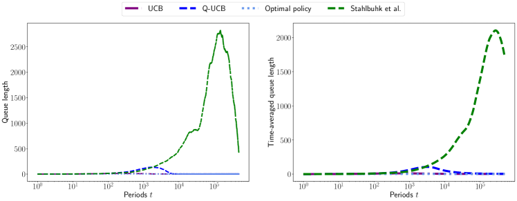
Figure 3: Expected per-period and time-averaged queue lengths of UCB, Q-UCB [KSJS21] and algorithm $\pi_{3}$ in [SSM21] in a single-queue setting with $K=5,\lambda=0.45,\boldsymbol{\mu}=(0.045,0.35,0.35,0.35,0.55)$; results are averaged over 50 runs.

A.3 Cost of learning for [NRP12]

The model in [NRP12] captures our single-queue multi-server setting by considering (in their notations) $N=1$ queue, fixed events $\beta(t)$ across time (so no information), action $k(t)$ corresponding the server chosen, and random events $\omega(t)$ is Bernoulli distributed with mean $\mu_{k(t)}$ where $\mu_{k}$’s are initially unknown. There is no utility to consider and we are focused on the queue length. Apply [NRP12, Theorems 1,2] to our single queue setting. In their notations, $\varepsilon_{\max}$ is equal to our slackness $\varepsilon$, and under the single-queue setting, we have $\tilde{K}=K$. To satisfy the condition that $\varepsilon_{Q}<\varepsilon_{\max}$ in [NRP12, Theorem 1] by their guarantee in Theorem 2, one needs to set a window size $W=\Theta(\frac{K^{2}}{\varepsilon^{2}})$, which set their constant $C=\Theta(\frac{K^{4}}{\varepsilon^{2}})$. Putting $C$ back into their Theorem 1 shows that the limited time-averaged queue length scales at least $O(\frac{K^{4}}{\varepsilon^{3}}).$

A.4 Cost of learning for [YSY23]

For a stationary multi-server system with $N$ agents and $M$ workers, the guarantee in [YSY23, Theorem 1] can be translated into a CLQ bound of $\Theta(\frac{N^{4}M^{4}}{\varepsilon^{3}})$. To see this, on the top right of page 6 in [YSY23], the authors derive an any-time time-averaged queue length bound of $O(I^{2}J^{2}g(\gamma)/\delta_{\max})$, where $I,J$ correspond to $N,M$ here, $\delta_{\max}$ is equal to $\varepsilon$ in our paper, and $g(\gamma)$ is at least $I^{2}J^{2}/\delta_{\max}$ by the requirement in [YSY23, Theorem 1]. Putting these together gives the CLQ bound. Note that our guarantee for MW-UCB in Theorem 4 corresponds to a CLQ bound of $\tilde{O}(\frac{N^{3.5}M^{3}}{\varepsilon})$; see the discussion in Appendix B.

A.5 Cost of learning for [FLW23]

For a bipartite queueing system with $N$ agents and $M$ workers, [FLW23, Theorem 3] shows a queue length bound of $\tilde{O}(\frac{M^{3}}{\varepsilon^{3}}+\frac{(ML_{\text{epoch})^{2}}}{\varepsilon^{2}T})$ for the expected time-averaged queue length of horizon $T$ (note that queue lengths are weighted by arrival rates in their bound). By Eq. (2) in [FLW23], $L_{\text{epoch}}=\tilde{O}(\frac{M^{2}}{\varepsilon^{2}})$. As a result, their queue length bound gives a CLQ bound of $\tilde{\Theta}(\frac{M^{3}}{\varepsilon^{3}}+\frac{M^{6}}{\varepsilon^{6}T}).$ Since the time-averaged queue length is at most $O(T)$, one can get a CLQ bound of $\tilde{O}(\frac{M^{3}}{\varepsilon^{3}})$. Our Theorem 4 gives a CLQ bound of $\tilde{O}(\frac{N^{1.5}M^{3}}{\varepsilon})$ by the mapping we provide in Appendix B.

A.6 Cost of learning for [NM23]

[NM23, Corollary 1] gives a queue length bound for their algorithm. The proof of this Corollary in [NM23, Appendix E] shows that the bound is about $\tilde{O}(\tau)$ where $\tau$ is a parameter such that $\varepsilon\gtrapprox\mu_{\min}\tau^{-1/3}$ in the stationary setting and $\mu_{\min}$ is $\min_{k\in\mathcal{K}}\mu_{k}$. Therefore, their queue length bound at best shows a CLQ of $\tilde{O}(\frac{1}{(\varepsilon\min_{k\in\mathcal{K}}\mu_{k})^{3}})$.

Appendix B Additional details for queueing network examples (Section 2.2)

We discuss in detail how examples discussed in Section 2.2 can be captured in our queueing network formulation. In a bipartite queueing system [FLW23], there are $N$ agents and $M$ workers. In period $t$, a new job arrives to each agent $n$’s queue with probability $\lambda_{n}$. The DM selects a matching $\sigma_{n,m}$ between agents and workers such that $\sum_{m’\in[M]}\sigma_{n,m’}\leq 1,\sum_{n’\in[N]}$ for all $n\in[N]$ and $\sigma_{n’,m}\leq 1$ for all $m\in[M]$. If $\sigma_{n,m}=1$, then the first job in agent $n$’s queue (if any) is cleared with probability $\mu_{n,m}$. Otherwise, the job stays in the queue. All arrivals and services are independent across queues, servers and periods. To translate this model into our queueing network formulation, let $\mathcal{N}=[N],\mathcal{K}=[N]\times[M]=\{(n,m),n\in[N],m\in[M]\}$. $\Lambda$ corresponds to $N$ independent Bernoulli random variables. For each $k=(n,m)\in\mathcal{K}$, we have $\mu_{k}=\mu_{n,m}$. The set $\mathcal{A}=\{0,1\}^{\mathcal{N}}$. $\Sigma$ is the set of subsets $\boldsymbol{\sigma}$ of $\mathcal{K}$, such that $\sum_{k=(n,m’)}\sigma_{k}\leq 1,\sum_{k=(n’,m)}\sigma_{k}\leq 1,\forall n\in[N],m\in[M]$. $\mathcal{B}_{n}=\{k=(n,m),m\in[M]\}$. $\mathcal{D}_{n}=\emptyset$ for all $n$, and $P$ only includes transitions to the virtual queue.

The multi-server system [YSY23] is similarly defined but instead of selecting a matching between agents and workers, the DM can match an agent with multiple workers, as long as there are sufficiently many jobs assigned to different workers. Therefore, the only change compared with the bipartite queueing system would be that $\Sigma$ consists of all $\boldsymbol{\sigma}$ such that $\sum_{k=(n’,m)}\sigma_{k}\leq 1,\forall m\in[M]$.

Appendix C Lower bound result (Section 3)

C.1 Proof of the lower bound (Theorem 1)

Consider $K$ sequences of service rates $\{\boldsymbol{\mu}^{k}=(\mu_{j}^{k})_{j\in\mathcal{K}}\}_{k\in\mathcal{K}}$ such that $\mu_{j}^{k}=\frac{1}{2}-\varepsilon$ for $j\neq k$ and $\mu_{k}^{k}=\frac{1}{2}+\varepsilon$. The arrival rate is $\lambda=\frac{1}{2}$. Fix a policy $\pi$. Let $\mathbb{P}^{k}\{\cdot\}$ and $\mathbb{E}^{k}[\cdot]$ denote the probability distribution and the expectation when the service rate is set as $\boldsymbol{\mu}^{k}$. Our goal is to show that for a particular $T$, we have $\frac{1}{K}\sum_{k\in\mathcal{K}}\frac{\sum_{t=1}^{T}\left(\mathbb{E}^{k}[Q(t)]-\mathbb{E}^{k}[Q^{\star}(t)]\right)}{T}=\Omega(\frac{K}{\varepsilon})$ and thus $\textsc{CLQ}^{\mathrm{single}}(\lambda,\boldsymbol{\mu}^{k},\pi)=\Omega(\frac{K}{\varepsilon})$ for at least one $k\in\mathcal{K}$. This then implies $\textsc{CLQ}^{\mathrm{single}}(K,\varepsilon,\pi)=\Omega(\frac{K}{\varepsilon})$ since the traffic slackness of the system is $\varepsilon$ for every $\boldsymbol{\mu}^{k}$. For every $t$, define the arrival sequence $\boldsymbol{A}_{t}=(A(1),\ldots,A(t))$ and service sequence $\boldsymbol{S}_{t}=(S_{J(1)}(1),\ldots,S_{J(t)}(t))$. Without loss of generality, we assume that $\pi$ is a deterministic function such that for every $t$, it maps $(\boldsymbol{A}_{t-1},\boldsymbol{S}_{t-1})$ to a server from $\mathcal{K}\cup\{\perp\}$. The case where $\pi$ allows randomization does not affect the result by Fubini’s Theorem (see Section 3.3 of [BC12]). We denote the history $(\boldsymbol{A}_{t},\boldsymbol{S}_{t})$ by $\boldsymbol{H}_{t}$; the selected server $J(t)$ is a function of $\boldsymbol{H}_{t-1}$ since $\pi$ is a deterministic policy.

For any horizon $T$, let $N_{k}(T)$ be the random variable of the number of times the policy selects server $k$ in the first $T$ periods. Define a sequence of uniform service rates $\boldsymbol{\mu}^{\mathrm{unif}}$ where $\boldsymbol{\mu}^{\mathrm{unif}}_{j}=\frac{1}{2}-\varepsilon$ for $j\in\mathcal{K}$ and $\mathbb{P}^{\mathrm{unif}}\{\cdot\}$ and $\mathbb{E}^{\mathrm{unif}}[\cdot]$ are defined similarly as before. In the bandit setting, it was shown that $\mathbb{E}^{k}[N_{k}(T)]$ is not much greater than $\mathbb{E}^{\mathrm{unif}}[N_{k}(T)]$ [ACFS02]. The following lemma shows that this is also the case for the considered queueing system.

Lemma C.1.

For any $k\in\mathcal{K},\varepsilon\leq\frac{1}{4},T\geq 1$, we have $\mathbb{E}^{k}[N_{k}(T)]\leq\mathbb{E}^{\mathrm{unif}}[N_{k}(T)]+4\varepsilon T\sqrt{\mathbb{E}^{\mathrm{unif}}[N_{k}(T)]}$.

Proof.

The proof is similar to that of Lemma A.1 in [ACFS02] and is based on KL divergence. We provide a detailed proof here because we use a different setting of service rates and because of the presence of arrival events. Fix $k,\varepsilon,T$. For ease of notations, we denote $\boldsymbol{A}=\boldsymbol{A}_{T},\boldsymbol{S}=\boldsymbol{S}_{T}$ and let $\boldsymbol{H}=(\boldsymbol{A},\boldsymbol{S})$ denote the history of horizon $T$. The realization of $\boldsymbol{H}$ is denoted by $\boldsymbol{h}\in\{0,1\}^{2T}$. Then for any distribution $G,P$ on $\{0,1\}^{2T}$, we denote $D_{\mathrm{TV}}\left(G\parallel P\right)$ to be the total variation between $G,P$ defined by the maximum of $|G(\mathcal{E})-P(\mathcal{E})|$ for all measurable event $\mathcal{E}$. In addition, we use $D_{\mathrm{KL}}\left(G\parallel P\right)$ for the KL divergence between $G,P$ defined by $D_{\mathrm{KL}}\left(G\parallel P\right)=\sum_{\boldsymbol{h}\in\{0,1\}^{2T}}G(\boldsymbol{h})\ln\left(\frac{G(\boldsymbol{h})}{P(\boldsymbol{h})}\right)$. For any $t\leq T$, let $G(\boldsymbol{h}_{t})$ denote the marginal distributions over $\boldsymbol{H}_{t}$. The conditional KL divergence between them conditioned on the history $\boldsymbol{h}_{t-1}$, $D_{\mathrm{KL}}\left(G(\boldsymbol{h}_{t}|\boldsymbol{h}_{t-1})\parallel P(\boldsymbol{h}_{t}|\boldsymbol{h}_{t-1})\right)$ is defined as $\sum_{\boldsymbol{h}_{t}\in\{0,1\}^{2t}}G(\boldsymbol{h}_{t})\ln\frac{G(\boldsymbol{h}_{t}|\boldsymbol{h}_{t-1})}{P(\boldsymbol{h}_{t}|\boldsymbol{h}_{t-1})}$ with $\boldsymbol{h}_{t-1}$ being the first $t-1$ entries of $\boldsymbol{h}_{t}$.

To bound the difference between $\mathbb{E}^{k}[N_{k}(T)]$ and $\mathbb{E}^{\mathrm{unif}}[N_{k}(T)]$, note that $N_{k}(T)$ must be a deterministic function of the history $\boldsymbol{H}$ when the policy $\pi$ is fixed. Write it as a mapping $N_{k}\colon\{0,1\}^{2T}\to[0,T]$. Then

$$\mathbb{E}^{k}[N_{k}(T)]-\mathbb{E}^{\mathrm{unif}}[N_{k}(T)]=\sum_{\boldsymbol{h}\in\{0,1\}^{2T}}N_{k}(\boldsymbol{h})\left(\mathbb{P}^{k}\{\boldsymbol{h}\}-\mathbb{P}^{\mathrm{unif}}\{\boldsymbol{h}\}\right) \leq TD_{\mathrm{TV}}\left(\mathbb{P}^{\mathrm{unif}}\parallel\mathbb{P}^{k}\right)$$ (36)

$$\leq T\sqrt{\frac{D_{\mathrm{KL}}\left(\mathbb{P}^{\mathrm{unif}}\parallel\mathbb{P}^{k}\right)}{2}}$$

where the last inequality is by Pinsker’s Inequality (Fact 1).

By the chain rule of KL divergence (Fact 2) and the independence between the history up to period $t-1$ and the arrivals and services in period $t$,

$$D_{\mathrm{KL}}\left(\mathbb{P}^{\mathrm{unif}}\parallel\mathbb{P}^{k}\right) =\sum_{t=1}^{T}D_{\mathrm{KL}}\left(\mathbb{P}^{\mathrm{unif}}(\boldsymbol{h}_{t}|\boldsymbol{h}_{t-1})\parallel\mathbb{P}^{k}(\boldsymbol{h}_{t}|\boldsymbol{h}_{t-1})\right)$$

$$=\sum_{t=1}^{T}\sum_{\boldsymbol{h}_{t}\in\{0,1\}^{2t}}\mathbb{P}^{\mathrm{unif}}(\boldsymbol{h}_{t})\ln\left(\frac{\mathbb{P}^{\mathrm{unif}}(\boldsymbol{h}_{t}|\boldsymbol{h}_{t-1})}{\mathbb{P}^{k}(\boldsymbol{h}_{t}|\boldsymbol{h}_{t-1})}\right)$$

$$=\sum_{t=1}^{T}\sum\limits_{\begin{subarray}{c}\boldsymbol{h}_{t-1}\in\{0,1\}^{2(t-1)}\\ a,s\in\{0,1\},j\in\mathcal{K}\end{subarray}}\mathbb{P}^{\mathrm{unif}}(\boldsymbol{h}_{t-1})\mathbb{P}^{\mathrm{unif}}(A(t)=a,J(t)=j,S_{j}(t)=s|\boldsymbol{h}_{t-1})$$

$$\mspace{32.0mu}\cdot\ln\frac{\mathbb{P}^{\mathrm{unif}}(A(t)=a,J(t)=j,S_{j}(t)=s|\boldsymbol{h}_{t-1})}{\mathbb{P}^{k}(A(t)=a,J(t)=j,S_{j}(t)=s|\boldsymbol{h}_{t-1})}.$$

When $J(t)\neq k$, the probability of event $(A(t)=a,S_{j}(t)=s)$ is the same for both $\mathbb{P}^{\mathrm{unif}}$ and $\mathbb{P}^{k}$ condition on $\boldsymbol{h}_{t-1}$. As a result, the last term becomes zero. Letting $D_{\mathrm{KL}}\left(g\parallel p\right)$ for the KL divergence between two Bernoulli distributions with mean $g,p\in[0,1]$ respectively, we then have

$$D_{\mathrm{KL}}\left(\mathbb{P}^{\mathrm{unif}}\parallel\mathbb{P}^{k}\right) =\sum_{t=1}^{T}\mathbb{P}^{\mathrm{unif}}(J(t)=k)D_{\mathrm{KL}}\left(\nicefrac{{1}}{{2}}-\varepsilon\parallel\nicefrac{{1}}{{2}}+\varepsilon\right)$$

$$=\mathbb{E}^{\mathrm{unif}}[N_{k}(T)]D_{\mathrm{KL}}\left(\nicefrac{{1}}{{2}}-\varepsilon\parallel\nicefrac{{1}}{{2}}+\varepsilon\right)$$

$$\leq\mathbb{E}^{\mathrm{unif}}[N_{k}(T)]\frac{4\varepsilon^{2}}{(\nicefrac{{1}}{{2}}+\varepsilon)(\nicefrac{{1}}{{2}}-\varepsilon)}=\frac{64}{3}\varepsilon^{2}\mathbb{E}^{\mathrm{unif}}[N_{k}(T)],$$ (37)

where the last inequality is because of Fact 3 and the assumption that $\varepsilon\leq 0.25$. Combining (37) with (36), we have

$$\mathbb{E}^{k}[N_{k}(T)]-\mathbb{E}^{\mathrm{unif}}[N_{k}(T)]\leq T\sqrt{\frac{32}{3}\varepsilon^{2}\mathbb{E}^{\mathrm{unif}}[N_{k}(T)]}\leq 4\varepsilon T\sqrt{\mathbb{E}^{\mathrm{unif}}[N_{k}(T)]}.$$

∎

The following lemma gives an upper bound on the time-averaged queue length for the optimal policy over any horizon. For ease of notations, we use $Q^{\star}(t)=Q(t,\pi^{\star})$.

Lemma C.2.

For any $\lambda,\varepsilon\in(0,1]$ and $T\geq 1$, it holds that $\frac{1}{T}\sum_{t=1}^{T}\mathbb{E}\left[Q^{\star}(t)\right]\leq\frac{\lambda}{\varepsilon}+\frac{1}{2}$.

Proof.

For any period $t$, consider the Lyapunov function $V^{\star}(t)=(Q^{\star}(t))^{2}$. We can rewrite the queueing dynamic (1) by $Q^{\star}(t+1)=\max(0,Q^{\star}(t)-S_{k^{\star}}(t))+A(t)$. As a result,

$$\mathbb{E}\left[V^{\star}(t+1)-V^{\star}(t)\right] =\mathbb{E}\left[\left(\max(0,Q^{\star}(t)-S_{k^{\star}}(t))+A(t)\right)^{2}-(Q^{\star}(t))^{2}\right]$$

$$\leq\mathbb{E}\left[A^{2}(t)+S_{k^{\star}}^{2}(t)+2(A(t)-S_{k^{\star}}(t))Q^{\star}(t)\right]$$

$$=\lambda+\lambda+\varepsilon-2\varepsilon\mathbb{E}\left[Q^{\star}(t)\right]$$

$$=2\lambda+\varepsilon-2\varepsilon\mathbb{E}\left[Q^{\star}(t)\right]$$

where the first inequality can be verified by considering $Q^{\star}(t)=0$ or $Q^{\star}(t)\geq 1$. Then for any $T\geq 1$, since $Q(1)=0$, we have

$$0\leq\mathbb{E}\left[V^{\star}(T+1)\right]=\sum_{t=1}^{T}\mathbb{E}\left[V^{\star}(t+1)-V^{\star}(t)\right]\leq(2\lambda+\varepsilon)T-2\varepsilon\sum_{t=1}^{T}\mathbb{E}\left[Q^{\star}(t)\right],$$

which gives $\frac{1}{T}\sum_{t=1}^{T}\mathbb{E}\left[Q^{\star}(t)\right]\leq\frac{\lambda}{\varepsilon}+\frac{1}{2}$. ∎

We are ready to prove Theorem 1.

Proof of Theorem 1.

For a setting of service rates $\boldsymbol{\mu}^{k}$, the number of total serviced jobs in time horizon $T$ is $\mathbb{E}^{k}[\sum_{t=1}^{T}\mu^{k}_{J(t)}]=(\nicefrac{{1}}{{2}}+\varepsilon)\mathbb{E}^{k}[N_{k}(T)]+(\nicefrac{{1}}{{2}}-\varepsilon)(T-\mathbb{E}^{k}[N_{k}(T)])=(\nicefrac{{1}}{{2}}-\varepsilon)T+2\varepsilon\mathbb{E}^{k}[N_{k}(T)]$. By Lemma C.1, we have

$$\sum_{k\in\mathcal{K}}\mathbb{E}^{k}\left[\sum_{t=1}^{T}\mu^{k}_{J(t)}\right] =\sum_{k\in\mathcal{K}}\left((\nicefrac{{1}}{{2}}-\varepsilon)T+2\varepsilon\mathbb{E}^{k}[N_{k}(T)]\right)$$ (38)

$$\leq(\nicefrac{{1}}{{2}}-\varepsilon)KT+2\varepsilon\sum_{k\in\mathcal{K}}\left(\mathbb{E}^{\mathrm{unif}}[N_{k}(T)]+4\varepsilon T\sqrt{\mathbb{E}^{\mathrm{unif}}[N_{k}(T)]}\right)$$

$$\leq(\nicefrac{{1}}{{2}}-\varepsilon)KT+2\varepsilon T+8\varepsilon^{2}T\sqrt{KT}$$

where the last inequality is by $\sum_{k\in\mathcal{K}}\mathbb{E}^{\mathrm{unif}}[N_{k}(T)]\leq T$ and Cauchy-Schwarz inequality. Let $T_{1}=\lceil\frac{K}{(32\varepsilon)^{2}}\rceil$. For any $T\leq T_{1}$, by the queueing dynamic (1),

$$\frac{1}{K}\sum_{k\in\mathcal{K}}\mathbb{E}^{k}[Q(T)]\geq\frac{1}{K}\sum_{k\in\mathcal{K}}\left(\lambda T-\mathbb{E}^{k}\left[\sum_{t=1}^{T}\mu^{k}_{J(t)}\right]\right) \overset{\eqref{eq:upperbound-service}}{\geq}\frac{T}{2}-\frac{1}{K}\left((\nicefrac{{1}}{{2}}-\varepsilon)KT+2\varepsilon T+8\varepsilon^{2}T\sqrt{KT}\right)$$ (39)

$$\geq\frac{\varepsilon T}{2}-8\varepsilon^{2}T\sqrt{\frac{T}{K}}\geq\frac{\varepsilon T}{4}$$

where the second inequality is because $K\geq 4$ and the last inequality is because $8\varepsilon^{2}T\sqrt{\frac{T}{K}}\leq\frac{\varepsilon T}{4}$ for any $T\leq\frac{K}{(32\varepsilon)^{2}}$. Therefore, for any feasible policy $\pi$,

$$\textsc{CLQ}^{\mathrm{single}}(K,\varepsilon,\pi)\geq\frac{1}{K}\sum_{k\in\mathcal{K}}\textsc{CLQ}^{\mathrm{single}}(\lambda,\boldsymbol{\mu}^{k},\pi) \geq\frac{1}{K}\left(\frac{1}{T_{1}}\sum_{T=1}^{T_{1}}\left(\mathbb{E}^{k}[Q(T)]-\mathbb{E}^{k}[Q^{\star}(T)]\right)\right)$$

$$\geq\frac{\varepsilon T_{1}}{8}-\frac{1}{2\varepsilon}-\frac{1}{2}\geq\frac{\varepsilon}{8}\left(\frac{K}{(32\varepsilon)^{2}}\right)-\frac{1}{2\varepsilon}-1\geq\frac{K}{2^{14}\varepsilon}$$

where the third inequality is by Lemma C.2 and (39); the forth inequality is by the setting of $T_{1}$ and $\varepsilon\leq\frac{1}{4}$; and the last inequality is by $K\geq 2^{14}$. ∎

C.2 Comparison with the lower bound in [KSJS21] (Remark 1)

Let $\mu_{\min}=\min_{k}\mu_{k},\Delta=\min_{k\colon\mu_{k}\neq\mu^{\star}}\mu^{\star}-\mu_{k}$ and $D(\boldsymbol{\mu})=\frac{\Delta}{D_{\mathrm{KL}}\left(\mu_{\min}\parallel\frac{\mu^{\star}+1}{2}\right)}$. For any $\alpha-$consistent policy $\pi$ (see Definition 1 in [KSJS21]), [KSJS21, Propostion 3] establishes the following lower bound.

Proposition 2.

Given any single-queue system $(\lambda,\boldsymbol{\mu})$ and any $\alpha-$consistent policy $\pi$ and $\gamma>\frac{1}{1-\alpha}$, there exists constant $\tau,C_{1}$ independent of $\lambda,\boldsymbol{\mu}$ such that for $\eta=\frac{(K-1)D(\boldsymbol{\mu})}{2\max(C_{1}K^{\gamma},\tau)}$, if $\varepsilon<\eta$, then

$$\mathbb{E}\left[Q(t,\pi)-Q^{\star}(t)\right]\geq\frac{D(\boldsymbol{\mu})}{2}(K-1)\frac{\log t}{\log\log t}$$ (40)

for $t\in[\max(C_{1}K^{\gamma},\tau),(K-1)\frac{D(\boldsymbol{\mu})}{2\varepsilon}]$.

Applying the lower bound (40) gives a lower bound on CLQ that $\textsc{CLQ}^{\mathrm{single}}(\lambda,\boldsymbol{\mu},\pi)\geq\tilde{\Omega}(KD(\boldsymbol{\mu})).$ To compare the tightness of (40) with our bound (Theorem 1), it remains to compare $D(\boldsymbol{\mu})$ with $O(\frac{1}{\varepsilon})$. The following result shows that $D(\boldsymbol{\mu})\leq 9$ and thus the bound from [KSJS21] is weaker than ours when $\varepsilon$ is sufficiently small.

Proposition 3.

For any $\boldsymbol{\mu}$, we have $D(\boldsymbol{\mu})\leq 9.$

Proof.

Note that if $\Delta=0$, we simply have $D(\boldsymbol{\mu})=0$; so let us focus on $\Delta\in(0,\mu^{\star}]$. In addition, we have $\mu_{\min}\leq\mu^{\star}-\Delta\leq\frac{\mu^{\star}+1}{2}$ and thus $D(\boldsymbol{\mu})\leq\frac{\Delta}{D_{\mathrm{KL}}\left(\mu^{\star}-\Delta\parallel\frac{\mu^{\star}+1}{2}\right)}$. We next consider the minimum value of $D_{\mathrm{KL}}\left(\mu^{\star}-\Delta\parallel\frac{\mu^{\star}+1}{2}\right)$ when $\Delta$ is fixed but $\mu^{\star}$ is allowed to change.

Define the triangular discrimination $D_{\triangle}(g\|p)$ between two Bernoulli random variables of mean $g,p$ respectively by

$$D_{\triangle}(g\|p)\coloneqq\frac{(g-p)^{2}}{g+p}+\frac{(1-g-(1-p))^{2}}{1-g+1-p}.$$

Let $q=\frac{\mu^{\star}-1}{2}$. A refined Pinsker’s inequality (see [FK21, Eq.(16)] and [Top00]) shows

$$D_{\mathrm{KL}}\left(\mu^{\star}-\Delta\parallel\frac{\mu^{\star}+1}{2}\right) \geq\frac{1}{2}D_{\triangle}(\mu^{\star}-\Delta\|\frac{\mu^{\star}+1}{2})$$

$$=\frac{1}{2}D_{\triangle}(\mu^{\star}-\Delta\|\mu^{\star}-q)=\frac{(\Delta-q)^{2}}{(2+3q-\Delta)(\Delta-3q)}.$$ (41)

Since $1\geq\mu^{\star}\geq\Delta$, we require $q\in[\frac{\Delta-1}{2},0]$. We next consider the minimum value of $f(q)\coloneqq\frac{(\Delta-q)^{2}}{(2+3q-\Delta)(\Delta-3q)}$ for $q\in[\frac{\Delta-1}{2},0]$. Taking derivative of $f$ gives

$$f^{\prime}(q)=\frac{(-12\Delta-6)q^{2}+(16\Delta^{2}+4\Delta)q-4\Delta^{3}+2\Delta^{2}}{(2+3q-\Delta)^{2}(\Delta-3q)^{2}}.$$

Solving $f^{\prime}(q^{\star})=0$ gives $q^{\star}=\frac{4\Delta^{2}+\Delta\pm(2\Delta^{2}+2\Delta)}{6\Delta+3}$. There are two cases:

• $\Delta>0.5$. Then zero points of $f^{\prime}$ are all positive and thus $f^{\prime}(q)$ is negative for $q\leq 0$, implying that $f(q)$ is minimized at $q=0$ over $[\frac{\Delta-1}{2},0]$. For this case, $f(q)\geq\frac{\Delta^{2}}{(2-\Delta)\Delta}\geq\frac{\Delta}{2}$;

• $\Delta\leq 0.5$. There is one zero point $q^{\star}=\frac{2\Delta^{2}-\Delta}{6\Delta+3}$ for $f^{\prime}(q)$ over $q\leq 0$. One can verify that $q^{\star}\in[\frac{\Delta-1}{2},0]$. Therefore, over $[\frac{\Delta-1}{2},0]$,

  $$f(q)\geq f(q^{\star})=\frac{(4\Delta(\Delta+1)/(6\Delta+3))^{2}}{(2-2\Delta/(2\Delta+1))(2\Delta/(2\Delta+1)}\geq\frac{16\Delta(\Delta+1)^{2}}{36(2\Delta+1)}\geq\frac{\Delta}{9}.$$

Combining the above two cases and by (41), we have $D_{\mathrm{KL}}\left(\mu^{\star}-\Delta\parallel\frac{\mu^{*}+1}{2}\right)\geq\min_{q\in[\frac{\Delta-1}{2},0]f(q)}\geq\frac{\Delta}{9}$. Therefore, $D(\boldsymbol{\mu})\leq\frac{\Delta}{D_{\mathrm{KL}}\left(\mu^{\star}-\Delta\parallel\frac{\mu^{*}+1}{2}\right)}\leq 9$. ∎

Appendix D Additional proofs for Section 6

D.1 Queue length bound in the learning stage (Lemma 6.1)

For every $t$, define $\tilde{\sigma}(t)$ as the schedule in $\Sigma$ with the largest weight, i.e., $\tilde{\sigma}(t)\in\arg\max_{\sigma\in\boldsymbol{\Sigma}}W^{\mathrm{net}}_{\sigma}(t)$. Given that $\boldsymbol{\Sigma}_{t}$ may be a strict subset of $\boldsymbol{\Sigma}$, this schedule need not be feasible in period $t$ (it may schedule more jobs from a queue than the queue has). We first lower bound the weight under schedule $\boldsymbol{\sigma}(t)$ selected by BP-UCB by a coupling with $\tilde{\boldsymbol{\sigma}}(t)$; the proof resembles that of Lemma 5.4.

Lemma D.1.

For a period $t$, $\sum_{n\in\mathcal{N}}\lambda_{n}Q_{n}(t)-W^{\mathrm{net}}_{\boldsymbol{\sigma}(t)}(t)\leq-\varepsilon\sum_{n\in\mathcal{N}}Q_{n}(t)+M_{\boldsymbol{\Sigma},\boldsymbol{\mathcal{B}}}^{2}+\Delta^{\mathrm{net}}(t)\|\boldsymbol{Q}(t)\|_{\infty}$.

Proof.

Fix a period $t$. The positive traffic slackness, captured through $\boldsymbol{\lambda}+\varepsilon\bm{1}\in\mathcal{S}^{\mathrm{net}}(\boldsymbol{\mu},\boldsymbol{\Sigma},\boldsymbol{\mathcal{B}},\bm{P})$, guarantees that there exists a distribution $\phi$ over $\boldsymbol{\Sigma}$ such that for every queue $n$, we have

$$\lambda_{n}+\varepsilon\leq\sum_{\boldsymbol{\sigma}\in\boldsymbol{\Sigma}}\phi_{\boldsymbol{\sigma}}\left(\sum_{k\in\mathcal{B}_{n}}\sigma_{k}\mu_{k}-\sum_{k^{\prime}\in\mathcal{K}}\sigma_{k^{\prime}}\mu_{k^{\prime}}p_{k^{\prime},n}\right).$$

Multiplying both sides by $Q_{n}(t)$ and summing over all queues gives $\sum_{n\in\mathcal{N}}(\lambda_{n}+\varepsilon)Q_{n}(t)$

$$\leq\sum_{\boldsymbol{\sigma}\in\boldsymbol{\Sigma}}\phi_{\boldsymbol{\sigma}}\sum_{n\in\mathcal{N}}Q_{n}(t)\left(\sum_{k\in\mathcal{B}_{n}}\sigma_{k}\mu_{k}-\sum_{k^{\prime}\in\mathcal{K}}\sigma_{k^{\prime}}\mu_{k^{\prime}}p_{k^{\prime},n}\right) =\sum_{\boldsymbol{\sigma}\in\boldsymbol{\Sigma}}\phi_{\boldsymbol{\sigma}}W^{\mathrm{net}}_{\boldsymbol{\sigma}}(t)\leq W^{\mathrm{net}}_{\tilde{\boldsymbol{\sigma}}(t)}(t)$$ (42)

where the last inequality is because $\phi$ is a distribution and $\tilde{\boldsymbol{\sigma}}(t)$ is the schedule in $\boldsymbol{\Sigma}$ with the largest weight. As a result, $\sum_{n\in\mathcal{N}}\lambda_{n}Q_{n}(t)-W^{\mathrm{net}}_{\tilde{\boldsymbol{\sigma}}(t)}(t)\leq-\varepsilon\sum_{n\in\mathcal{N}}Q_{n}(t)$.

We next lower bound the weight of $\boldsymbol{\sigma}^{\textsc{BP}}(t)=\arg\max_{\boldsymbol{\sigma}\in\boldsymbol{\Sigma}_{t}}W^{\mathrm{net}}_{\boldsymbol{\sigma}}(t)$, the schedule with the largest weight over schedules in $\boldsymbol{\Sigma}_{t}$. We construct a schedule $\boldsymbol{\alpha}\in\boldsymbol{\Sigma}_{t}$ from $\tilde{\boldsymbol{\sigma}}(t)$. For a queue $n$, if $Q_{n}(t)\geq\sum_{k\in\mathcal{B}_{n}}\tilde{\boldsymbol{\sigma}}_{k}(t)$, we set $\alpha_{k}=\tilde{\boldsymbol{\sigma}}_{k}(t)$ for all $k\in\mathcal{B}_{n}$; otherwise, we set $\alpha_{k}=0$ for $k\in\mathcal{B}_{n}$. By construction we have $\boldsymbol{\alpha}\in\boldsymbol{\Sigma}_{t}$, and thus $W^{\mathrm{net}}_{\boldsymbol{\sigma}^{\textsc{BP}}(t)}(t)\geq W^{\mathrm{net}}_{\boldsymbol{\alpha}}(t)$. For a server $k$, let $i_{k}$ be the queue it belongs to and let $h_{n}=\mathbbm{1}\left(Q_{n}(t)<\sum_{k\in\mathcal{B}_{n}}\tilde{\sigma}_{k}(t)\right)$ for a queue $n$. Then

$$W^{\mathrm{net}}_{\boldsymbol{\sigma}^{\textsc{BP}}(t)}(t)\geq W^{\mathrm{net}}_{\boldsymbol{\alpha}}(t) =W^{\mathrm{net}}_{\tilde{\boldsymbol{\sigma}}(t)}(t)-\left(\sum_{n\in\mathcal{N}}h_{n}Q_{n}(t)\sum_{k\in\mathcal{B}_{n}}\tilde{\sigma}_{k}(t)\mu_{k}-\sum_{k^{\prime}\in\mathcal{K}}h_{i_{k^{\prime}}}\tilde{\sigma}_{k^{\prime}}(t)\mu_{k^{\prime}}\sum_{n\in\mathcal{N}}p_{k^{\prime},n}Q_{n}(t)\right)$$

$$\geq W^{\mathrm{net}}_{\tilde{\boldsymbol{\sigma}}(t)}(t)-\sum_{n\in\mathcal{N}}h_{n}Q_{n}(t)\sum_{k\in\mathcal{B}_{n}}\tilde{\sigma}_{k}(t)\mu_{k}$$

$$\geq W^{\mathrm{net}}_{\tilde{\boldsymbol{\sigma}}(t)}(t)-\sum_{n\in\mathcal{N}}\left(\sum_{k\in\mathcal{B}_{n}}\tilde{\sigma}_{k}(t)\mu_{k}\right)^{2}\geq W^{\mathrm{net}}_{\tilde{\boldsymbol{\sigma}}(t)}(t)-M_{\boldsymbol{\Sigma},\boldsymbol{\mathcal{B}}}^{2}.$$ (43)

We then finish the proof by recalling the definition of $\Delta^{\mathrm{net}}(t)$ in (33)

$$\sum_{n\in\mathcal{N}}\lambda_{n}Q_{n}(t)-W_{\boldsymbol{\sigma}(t)}^{\mathrm{net}}(t) \leq\sum_{n\in\mathcal{N}}\lambda_{n}Q_{n}(t)-W_{\boldsymbol{\sigma}^{\textsc{BP}}(t)}^{\mathrm{net}}(t)+\Delta^{\mathrm{net}}(t)\|\boldsymbol{Q}(t)\|_{\infty} \Delta^{\mathrm{net}}(t)$$ (Definition of )

$$\leq\sum_{n\in\mathcal{N}}\lambda_{n}Q_{n}(t)-W_{\tilde{\boldsymbol{\sigma}}(t)}^{\mathrm{net}}(t)+M_{\boldsymbol{\Sigma},\boldsymbol{\mathcal{B}}}^{2}+\Delta^{\mathrm{net}}(t)\|\boldsymbol{Q}(t)\|_{\infty}$$ (43)

$$\leq-\varepsilon\sum_{n\in\mathcal{N}}Q_{n}(t)+M_{\boldsymbol{\Sigma},\boldsymbol{\mathcal{B}}}^{2}+\Delta^{\mathrm{net}}(t)\|\boldsymbol{Q}(t)\|_{\infty},$$ (42)

which finishes the proof. ∎

Let $\mathcal{F}_{t}$ be the $\sigma-$field generated by the sample path before period $t$ (including arrivals $A_{n}(\tau)$, services $S_{k}(\tau)$ and transitions $L_{k,n}(\tau)$ for $\tau<t$). Then $\{\varphi(t)\},\{\Delta^{\mathrm{net}}(t)\}$ and $\{\boldsymbol{\sigma}(t)\}$ are $\{\mathcal{F}_{t}\}$-adapted process. We bound the maximum increase (decrease) of $\varphi(t)$ and its drift in the following lemma which is similar to Lemma 5.5.

Lemma D.2.

For the process $\{\varphi(t)\}$, we have that for every period $t$,

1. Bounded difference: $|\varphi(t+1)-\varphi(t)|\leq\sqrt{2M_{\boldsymbol{\mathcal{A}}}+3M_{\boldsymbol{\Sigma},\boldsymbol{\mathcal{B}}}^{2}}$;

2. Drift bound: $\mathbb{E}\left[\varphi(t+1)-\varphi(t)\,\middle|\,\mathcal{F}_{t}\right]\leq-\frac{\varepsilon}{4}+\left(\Delta^{\mathrm{net}}(t)-\frac{\varepsilon}{2}\right)^{+}$ if $\varphi(t)\geq\frac{8(M_{\boldsymbol{\mathcal{A}}}+2M_{\boldsymbol{\Sigma},\boldsymbol{\mathcal{B}}}^{2})}{\varepsilon}$.

Proof.

Fix a period $t$. By triangle inequality, $|\varphi(t+1)-\varphi(t)|=|\|\boldsymbol{Q}(t+1)\|_{2}-\|\boldsymbol{Q}(t)\|_{2}|\leq\|\boldsymbol{Q}(t+1)-\boldsymbol{Q}(t)\|_{2}$ and

$$\|\boldsymbol{Q}(t+1)-\boldsymbol{Q}(t)\|_{2} =\sqrt{\sum_{n\in\mathcal{N}}\left(-\sum_{k\in\mathcal{B}_{n}}\sigma_{k}(t)S_{k}(t)+A_{n}(t)+\sum_{k^{\prime}\in\mathcal{K}}\sigma_{k^{\prime}}(t)S_{k^{\prime}}(t)L_{k^{\prime},n}(t)\right)^{2}}$$ (by the queueing dynamic (3))

$$\leq\sqrt{\sum_{n\in\mathcal{N}}\left(\left(A_{n}(t)+\sum_{k^{\prime}\in\mathcal{K}}\sigma_{k^{\prime}}(t)S_{k^{\prime}}(t)L_{k^{\prime},n}(t)\right)^{2}+\left(\sum_{k\in\mathcal{B}_{n}}\sigma_{k}(t)S_{k}(t)\right)^{2}\right)}$$

$$\leq\sqrt{2\sum_{n\in\mathcal{N}}A_{n}(t)+2\left(\sum_{n\in\mathcal{N}}\sum_{k^{\prime}\in\mathcal{K}}\sigma_{k^{\prime}}(t)S_{k^{\prime}}(t)L_{k^{\prime},n}(t)\right)^{2}+M_{\boldsymbol{\Sigma},\boldsymbol{\mathcal{B}}}^{2}}$$

$$\leq\sqrt{2M_{\boldsymbol{\mathcal{A}}}+2\left(\sum_{k^{\prime}\in\mathcal{K}}\sigma_{k^{\prime}}(t)S_{k^{\prime}}(t)\right)^{2}+M_{\boldsymbol{\Sigma},\boldsymbol{\mathcal{B}}}^{2}}$$

$$\leq\sqrt{2M_{\boldsymbol{\mathcal{A}}}+2M_{\boldsymbol{\Sigma},\boldsymbol{\mathcal{B}}}^{2}+M_{\boldsymbol{\Sigma},\boldsymbol{\mathcal{B}}}^{2}}=\sqrt{2M_{\boldsymbol{\mathcal{A}}}+3M_{\boldsymbol{\Sigma},\boldsymbol{\mathcal{B}}}^{2}}.$$ (44)

To bound the drift condition on $\mathcal{F}_{t}$, we again use Fact 6 that for $\|\boldsymbol{Q}(t)\|_{2}>0$, we have

$$\|\boldsymbol{Q}(t+1)\|_{2}\leq\|\boldsymbol{Q}(t)\|_{2}+\frac{\boldsymbol{Q}(t)\cdot(\boldsymbol{Q}(t+1)-\boldsymbol{Q}(t))+\|\boldsymbol{Q}(t+1)-\boldsymbol{Q}(t)\|_{2}^{2}}{\|\boldsymbol{Q}(t)\|_{2}}.$$ (45)

Condition on $\mathcal{F}_{t}$ and suppose $\varphi(t)\geq\frac{8(M_{\boldsymbol{\mathcal{A}}}+2M_{\boldsymbol{\Sigma},\boldsymbol{\mathcal{B}}}^{2})}{\varepsilon}$. We first bound

$$\hskip 14.45377pt\mathbb{E}\left[\boldsymbol{Q}(t)\cdot(\boldsymbol{Q}(t+1)-\boldsymbol{Q}(t))\,\middle|\,\mathcal{F}_{t}\right]$$

$$=\mathbb{E}\left[\sum_{n\in\mathcal{N}}Q_{n}(t)\left(A_{n}(t)-\sum_{k\in\mathcal{B}_{n}}\sigma_{k}(t)S_{k}(t)+\sum_{k^{\prime}\in\mathcal{K}}\sigma_{k^{\prime}}(t)S_{k^{\prime}}(t)L_{k^{\prime},n}(t)\right)\,\middle|\,\mathcal{F}_{t}\right]$$ (by (3))

$$=\sum_{n\in\mathcal{N}}Q_{n}(t)\left(\lambda_{n}-\sum_{k\in\mathcal{B}_{n}}\sigma_{k}(t)\mu_{k}+\sum_{k^{\prime}\in\mathcal{K}}\sigma_{k^{\prime}}(t)\mu_{k^{\prime}}p_{k^{\prime},n}\right)$$ (arrivals, services and transitions in a period are independent of the history)

$$=\sum_{n\in\mathcal{N}}\lambda_{n}Q_{n}(t)-W^{\mathrm{net}}_{\boldsymbol{\sigma}(t)}(t)$$

$$\leq-\varepsilon\sum_{n\in\mathcal{N}}Q_{n}(t)+M_{\boldsymbol{\Sigma},\boldsymbol{\mathcal{B}}}^{2}+\Delta^{\mathrm{net}}(t)\|\boldsymbol{Q}(t)\|_{\infty}$$ (46)

where the last inequality is by Lemma D.1. We then have

$$\mathbb{E}\left[\varphi(t+1)-\varphi(t)\,\middle|\,\mathcal{F}_{t}\right] \leq\mathbb{E}\left[\frac{\boldsymbol{Q}(t)\cdot(\boldsymbol{Q}(t+1)-\boldsymbol{Q}(t))+\|\boldsymbol{Q}(t+1)-\boldsymbol{Q}(t)\|_{2}^{2}}{\|\boldsymbol{Q}(t)\|_{2}}\,\middle|\,\mathcal{F}_{t}\right]$$ (by (45))

$$\leq\mathbb{E}\left[\frac{\boldsymbol{Q}(t)\cdot(\boldsymbol{Q}(t+1)-\boldsymbol{Q}(t))}{\|\boldsymbol{Q}(t)\|_{2}}\,\middle|\,\mathcal{F}_{t}\right]+\frac{2M_{\boldsymbol{\mathcal{A}}}+3M_{\boldsymbol{\Sigma},\boldsymbol{\mathcal{B}}}^{2}}{\|\boldsymbol{Q}(t)\|_{2}}$$ (by (44))

$$\leq\frac{-\varepsilon\sum_{n\in\mathcal{N}}Q_{n}(t)+M_{\boldsymbol{\Sigma},\boldsymbol{\mathcal{B}}}^{2}+\Delta^{\mathrm{net}}(t)\|\boldsymbol{Q}(t)\|_{\infty}}{\|\boldsymbol{Q}(t)\|_{2}}+\frac{2M_{\boldsymbol{\mathcal{A}}}+3M_{\boldsymbol{\Sigma},\boldsymbol{\mathcal{B}}}^{2}}{\|\boldsymbol{Q}(t)\|_{2}} \boldsymbol{Q}(t)\in\mathcal{F}_{t}$$ (by (46) and that )

$$\leq-\varepsilon+\Delta^{\mathrm{net}}(t)+\frac{2M_{\boldsymbol{\mathcal{A}}}+4M_{\boldsymbol{\Sigma},\boldsymbol{\mathcal{B}}}^{2}}{\|\boldsymbol{Q}(t)\|_{2}} \|\boldsymbol{Q}(t)\|_{1}\geq\|\boldsymbol{Q}(t)\|_{2}\geq\|\boldsymbol{Q}(t)\|_{\infty}$$ ()

$$\leq-\frac{\varepsilon}{2}+(\Delta^{\mathrm{net}}(t)-\frac{\varepsilon}{2})^{+}+\frac{\varepsilon}{4} \varphi(t)\geq\frac{8(M_{\boldsymbol{\mathcal{A}}}+2M_{\boldsymbol{\Sigma},\boldsymbol{\mathcal{B}}}^{2})}{\varepsilon}$$ (assumption that )

$$=-\frac{\varepsilon}{4}+(\Delta^{\mathrm{net}}(t)-\frac{\varepsilon}{2})^{+},$$

which finishes the proof. ∎

We next show an upper bound on $\Delta^{\mathrm{net}}(t)$.

Lemma D.3.

For every period $t$, $\Delta^{\mathrm{net}}(t)\leq 2M_{\boldsymbol{\Sigma},\boldsymbol{\mathcal{B}}}$.

Proof.

If $\|\boldsymbol{Q}(t)\|_{\infty}=0$, then $\Delta^{\mathrm{net}}(t)=0$; otherwise,

$$\Delta^{\mathrm{net}}(t) =\frac{W^{\mathrm{net}}_{\boldsymbol{\sigma}^{\textsc{BP}}(t)}(t)-W^{\mathrm{net}}_{\boldsymbol{\sigma}(t)}(t)}{\|\boldsymbol{Q}(t)\|_{\infty}}$$

$$=\frac{\sum_{n\in\mathcal{N}}Q_{n}(t)\left(\sum_{k\in\mathcal{B}_{n}}\left(\sigma^{\textsc{BP}}_{k}(t)-\sigma_{k}(t)\right)\mu_{k}-\sum_{k^{\prime}\in\mathcal{K}}\left(\sigma^{\textsc{BP}}_{k^{\prime}}(t)-\sigma_{k^{\prime}}(t)\right)\mu_{k^{\prime}}p_{k^{\prime},n}\right)}{\|\boldsymbol{Q}(t)\|_{\infty}}$$

$$\leq\frac{\sum_{n\in\mathcal{N}}Q_{n}(t)\left(\sum_{k\in\mathcal{B}_{n}}\sigma^{\textsc{BP}}_{k}(t)\mu_{k}+\sum_{k^{\prime}\in\mathcal{K}}\sigma_{k^{\prime}}(t)\mu_{k^{\prime}}p_{k^{\prime},n}\right)}{\|\boldsymbol{Q}(t)\|_{\infty}}$$

$$\leq\sum_{n\in\mathcal{N}}\left(\sum_{k\in\mathcal{B}_{n}}\sigma^{\textsc{BP}}_{k}(t)\mu_{k}+\sum_{k^{\prime}\in\mathcal{K}}\sigma_{k^{\prime}}(t)\mu_{k^{\prime}}p_{k^{\prime},n}\right)$$

$$\leq\sum_{k\in\mathcal{K}}\sigma_{k}^{\textsc{BP}}(t)+\sum_{k^{\prime}\in\mathcal{K}}\sigma_{k^{\prime}}(t)\sum_{n\in\mathcal{N}}p_{k^{\prime},n}$$

$$\leq\sum_{k\in\mathcal{K}}\sigma_{k}^{\textsc{BP}}(t)+\sum_{k^{\prime}\in\mathcal{K}}\sigma_{k^{\prime}}(t) p_{k^{\prime},\cdot} \mathcal{N}\cup\{\perp\}$$ (since is a probability distribution over )

$$\leq 2M_{\boldsymbol{\Sigma},\boldsymbol{\mathcal{B}}}.$$

∎

The proof of Lemma 6.1 combines Lemmas D.2, D.3 and  5.7.

Proof of Lemma 6.1.

To apply Lemma 5.7, wet set $\Psi(t)=\varphi(t),Z(t)=\left(\Delta^{\mathrm{net}}(t)-\frac{\varepsilon}{2}\right)^{+}$. To verify the condition of Lemma 5.7, take $\kappa=\sqrt{2M_{\boldsymbol{\mathcal{A}}}+4M_{\boldsymbol{\Sigma},\boldsymbol{\mathcal{B}}}^{2}},\delta=\varepsilon/4,B=\frac{8(M_{\boldsymbol{\mathcal{A}}}+2M_{\boldsymbol{\Sigma},\boldsymbol{\mathcal{B}}}^{2})}{\varepsilon}$. By Lemma D.2, we have $|\Psi(t+1)-\Psi(t)|\leq\kappa$ with probability one and $\mathbb{E}\left[\Psi(t+1)-\Psi(t)\,\middle|\,\mathcal{F}_{t}\right]\leq-\delta+Z(t)$ if $\Psi(t)\geq B$. Lemma D.3 shows $Z(t)\leq\Delta^{\mathrm{net}}(t)\leq 2M_{\boldsymbol{\Sigma},\boldsymbol{\mathcal{B}}}\leq\kappa$. For a horizon $T$, using Lemma 5.7 to $\varphi(t)$ for $t\leq T$ and taking average,

$$\frac{\sum_{t=1}^{T}\mathbb{E}\left[\|\boldsymbol{Q}(t)\|_{2}\right]}{T} =\frac{\sum_{t=1}^{T}\mathbb{E}\left[\Psi(t)\right]}{T} \Psi(t)=\varphi(t)=\|\boldsymbol{Q}(t)\|_{2}$$ (Definition of )

$$\leq 4\kappa+B+\frac{2\kappa^{2}}{\delta}+\mathbb{E}\left[\sum_{t=1}^{T-1}Z(t)\right]$$ (Lemma 5.7)

$$=4\sqrt{2M_{\boldsymbol{\mathcal{A}}}+4M_{\boldsymbol{\Sigma},\boldsymbol{\mathcal{B}}}^{2}}+\frac{8(M_{\boldsymbol{\mathcal{A}}}+2M_{\boldsymbol{\Sigma},\boldsymbol{\mathcal{B}}}^{2})}{\varepsilon}++\frac{16M_{\boldsymbol{\mathcal{A}}}+32M_{\boldsymbol{\Sigma},\boldsymbol{\mathcal{B}}}^{2}}{\varepsilon}+\mathbb{E}\left[\sum_{t=1}^{T-1}\left(\Delta^{\mathrm{net}}(t)-\varepsilon/2\right)^{+}\right]$$

$$\leq\frac{32M_{\boldsymbol{\mathcal{A}}}+64M_{\boldsymbol{\Sigma},\boldsymbol{\mathcal{B}}}^{2}}{\varepsilon}+\mathrm{SaR}^{\mathrm{net}}(\pi,T),$$

which finishes the proof. ∎

D.2 Queue length bound in the regenerate stage (Lemma 6.2)

We first show that Lemma 5.9 will still hold for a queueing network.

Lemma D.4.

For any horizon $T$ and every sample path, we have $\sum_{t=1}^{T}\|\boldsymbol{Q}(t)\|_{1}\geq\frac{(\max_{t=1}^{T}\|\boldsymbol{Q}(t)\|_{1})^{2}}{4M_{\boldsymbol{\mathcal{A}}}}$.

Proof.

It suffices to prove that for every period $t$, we have $\|\boldsymbol{Q}(t+1)\|_{1}\leq\|\boldsymbol{Q}(t)\|_{1}+M_{\boldsymbol{\mathcal{A}}}$, as we can then follow the proof of Lemma 5.9 to finish the proof. Now to show the bound on the increase, by the queueing dynamic (3), we bound in period $t$,

$$\|\boldsymbol{Q}(t+1)\|_{1} =\sum_{n\in\mathcal{N}}\left(Q_{n}(t)-\sum_{k\in\mathcal{B}_{n}}\sigma_{k}(t)S_{k}(t)+A_{n}(t)+\sum_{k^{\prime}\in\mathcal{K}}\sigma_{k^{\prime}}(t)S_{k^{\prime}}(t)L_{k^{\prime},n}(t)\right)$$ (by (3) and summing over all queues)

$$=\sum_{n\in\mathcal{N}}Q_{n}(t)+\sum_{n\in\mathcal{N}}A_{n}(t)+\sum_{k\in\mathcal{K}}\sigma_{k}(t)S_{k}(t)\left(1-\sum_{n\in\mathcal{N}}L_{k,n}(t)\right)$$

$$\leq\sum_{n\in\mathcal{N}}Q_{n}(t)+\sum_{n\in\mathcal{N}}A_{n}(t) \sum_{n\in\mathcal{N}}L_{k,n}\leq 1$$ ( since a job transits to either a queue or leaves the system)

$$\leq\|\boldsymbol{Q}(t)\|_{1}+M_{\boldsymbol{\mathcal{A}}},$$

which completes the proof by following arguments in the second paragraph of the proof of Lemma 5.9. ∎

Proof of Lemma 6.2.

Fix a period $t$. First, we use equation (54) from the proof of Fact 6

$$\|\boldsymbol{Q}(t)\|_{2}^{2}+2\boldsymbol{Q}(t)\cdot\left(\boldsymbol{Q}(t+1)-\boldsymbol{Q}(t)\right)+\|\boldsymbol{Q}(t+1)-\boldsymbol{Q}(t)\|_{2}^{2}=\|\boldsymbol{Q}(t+1)\|_{2}^{2}.$$

As a result,

$$\mathbb{E}\left[V(t+1)-V(t)\,\middle|\,\mathcal{F}_{t}\right] =\mathbb{E}\left[\|\boldsymbol{Q}(t+1)\|_{2}^{2}-\|\boldsymbol{Q}(t)\|_{2}^{2}\,\middle|\,\mathcal{F}_{t}\right]$$

$$=\mathbb{E}\left[2\boldsymbol{Q}(t)\cdot\left(\boldsymbol{Q}(t+1)-\boldsymbol{Q}(t)\right)+\|\boldsymbol{Q}(t+1)-\boldsymbol{Q}(t)\|_{2}^{2}\,\middle|\,\mathcal{F}_{t}\right]$$

$$\leq\mathbb{E}\left[2\boldsymbol{Q}(t)\cdot\left(\boldsymbol{Q}(t+1)-\boldsymbol{Q}(t)\right)\,\middle|\,\mathcal{F}_{t}\right]+2M_{\boldsymbol{\mathcal{A}}}+3M_{\boldsymbol{\Sigma},\boldsymbol{\mathcal{B}}}^{2}$$ (by (44))

$$\leq 2\left(-\varepsilon\sum_{n\in\mathcal{N}}Q_{n}(t)+M_{\boldsymbol{\Sigma},\boldsymbol{\mathcal{B}}}^{2}+\Delta^{\mathrm{net}}(t)\|\boldsymbol{Q}(t)\|_{\infty}\right)+2M_{\boldsymbol{\mathcal{A}}}+3M_{\boldsymbol{\Sigma},\boldsymbol{\mathcal{B}}}^{2}.$$ (by (46))

Take expectation on both sides gives

$$\mathbb{E}\left[V(t+1)\right]-\mathbb{E}\left[V(t)\right]\leq\mathbb{E}\left[-2\varepsilon\|\boldsymbol{Q}(t)\|_{1}+2\Delta^{\mathrm{net}}(t)\|\boldsymbol{Q}(t)\|_{\infty}\right]+2M_{\boldsymbol{\mathcal{A}}}+5M_{\boldsymbol{\Sigma},\boldsymbol{\mathcal{B}}}^{2}.$$ (47)

Then for a fixed horizon $T$, we have

$$0 \leq\mathbb{E}\left[V(T+1)\right]-\mathbb{E}\left[V(1)\right] V(T+1)\geq 0 V(1)=0$$ (since and )

$$=\sum_{t=1}^{T}\mathbb{E}\left[V(t+1)-V(t)\right]$$

$$\leq\mathbb{E}\left[-2\varepsilon\sum_{t=1}^{T}\|\boldsymbol{Q}(t)\|_{1}+2\sum_{t=1}^{T}\Delta^{\mathrm{net}}(t)\|\boldsymbol{Q}(t)\|_{\infty}\right]+T(2M_{\boldsymbol{\mathcal{A}}}+5M_{\boldsymbol{\Sigma},\boldsymbol{\mathcal{B}}}^{2})$$

$$\leq-\varepsilon\mathbb{E}\left[\sum_{t=1}^{T}\|\boldsymbol{Q}(t)\|_{1}\right]+2\mathbb{E}\left[\sum_{t=1}^{T}\left(\Delta^{\mathrm{net}}(t)-\frac{\varepsilon}{2}\right)^{+}\|\boldsymbol{Q}(t)\|_{1}\right]+T(2M_{\boldsymbol{\mathcal{A}}}+5M_{\boldsymbol{\Sigma},\boldsymbol{\mathcal{B}}}^{2})$$

$$=-\frac{\varepsilon}{2}\mathbb{E}\left[\sum_{t=1}^{T}\|\boldsymbol{Q}(t)\|_{1}\right]+\mathbb{E}\left[-\frac{\varepsilon}{2}\sum_{t=1}^{T}\|\boldsymbol{Q}(t)\|_{1}+2\sum_{t=1}^{T}\left(\Delta^{\mathrm{net}}(t)-\frac{\varepsilon}{2}\right)^{+}\|\boldsymbol{Q}(t)\|_{1}\right]+T(2M_{\boldsymbol{\mathcal{A}}}+5M_{\boldsymbol{\Sigma},\boldsymbol{\mathcal{B}}}^{2})$$ (48)

We show a sample path upper bound of the second term by seeing that

$$\hskip 14.45377pt-\frac{\varepsilon}{2}\sum_{t=1}^{T}\|\boldsymbol{Q}(t)\|_{1}+2\sum_{t=1}^{T}\left(\Delta^{\mathrm{net}}(t)-\frac{\varepsilon}{2}\right)^{+}\|\boldsymbol{Q}(t)\|_{1}$$

$$\leq-\frac{\varepsilon}{2}\sum_{t=1}^{T}\|\boldsymbol{Q}(t)\|_{1}+2\left(\max_{t\leq T}\|\boldsymbol{Q}(t)\|_{1}\right)\sum_{t=1}^{T}\left(\Delta^{\mathrm{net}}(t)-\frac{\varepsilon}{2}\right)^{+}$$

$$\leq-\frac{\varepsilon\left(\max_{t\leq T}\|\boldsymbol{Q}(t)\|_{1}\right)^{2}}{8M_{\boldsymbol{\mathcal{A}}}}+2\left(\max_{t\leq T}\|\boldsymbol{Q}(t)\|_{1}\right)\mathrm{SaR}^{\mathrm{net}}(\pi,T)$$ (by Lemma D.4 and the definition of satisficing regret)

$$\leq\frac{8M_{\boldsymbol{\mathcal{A}}}\mathrm{SaR}^{\mathrm{net}}(\pi,T)^{2}}{\varepsilon}$$ (49)

where the last inequality uses the fact that $-ax^{2}+bx\leq\frac{b^{2}}{4a}$ for any $a<0$ and takes $x=\max_{t\leq T}\|\boldsymbol{Q}(t)\|_{1}$. Replacing the second term in (48) by the upper bound in (49) gives

$$0\leq-\frac{\varepsilon}{2}\mathbb{E}\left[\sum_{t=1}^{T}\|\boldsymbol{Q}(t)\|_{1}\right]+\frac{8M_{\boldsymbol{\mathcal{A}}}\mathbb{E}\left[\mathrm{SaR}^{\mathrm{net}}(\pi,T)^{2}\right]}{\varepsilon}+T(2M_{\boldsymbol{\mathcal{A}}}+5M_{\boldsymbol{\Sigma},\boldsymbol{\mathcal{B}}}^{2}).$$

Dividing both sides by $T$ and reorganizing terms show

$$\frac{\mathbb{E}\left[\sum_{t=1}^{T}\|\boldsymbol{Q}(t)\|_{1}\right]}{T}\leq\frac{4M_{\boldsymbol{\mathcal{A}}}+10M_{\boldsymbol{\Sigma},\boldsymbol{\mathcal{B}}}^{2}}{\varepsilon}+\frac{16M_{\boldsymbol{\mathcal{A}}}}{\varepsilon^{2}}\frac{\mathbb{E}\left[\mathrm{SaR}^{\mathrm{net}}(\pi,T)^{2}\right]}{T}.$$

∎

D.3 Satisficing regret of BP-UCB (Lemma 6.3)

The proof of Lemma 6.3 follows a similar structure as that of Lemma 5.3. The additional complexity comes from estimating $r_{k,n}=\mu_{k}p_{k,n}$, the probability a job transitions to $n$ given that server $k$ is selected. We define $\Delta_{k}(t)=\sqrt{\frac{2\ln t}{C_{k}(t)}}$ as the confidence bound of server $k$ in period $t$ as in BP-UCB (Algorithm 3) and let $\mathcal{G}_{t}$ be the good event that $\left\{\Delta^{\mathrm{net}}(t)\leq 4\sum_{k\in\mathcal{K}}\sigma_{k}(t)\Delta_{k}(t)|\mathcal{D}_{k}|\right\}$. Extending Lemma 5.10, we show the following lower bound on $\mathbb{P}\{\mathcal{G}_{t}\}$.

Lemma D.5.

For every period $t$ and under BP-UCB, we have $\mathbb{P}\{\mathcal{G}_{t}\}\geq 1-4\sum_{k\in\mathcal{K}}|\mathcal{D}_{k}|t^{-3}$.

Proof.

Fix a period $t$. Define the event $\mathcal{E}_{t}$ as the case that all sample averages are within a confidence bound of their true values:

$$\mathcal{C}_{t}=\left\{\forall_{n\in\mathcal{N},k\in\mathcal{K}},|\hat{\mu}_{k}(t)-\mu_{k}|\leq\Delta_{k}(t),|\hat{r}_{k,n}(t)-r_{k,n}(t)|\leq\Delta_{k}(t)\right\}.$$

We first lower bound the probability of $\mathcal{C}_{t}$. For a server $k$, condition on $C_{k}(t)=c\in\{0,1,\ldots,t-1\}$. By Hoeffding’s inequality (Fact 4), we have

$$\mathbb{P}\left\{|\hat{\mu}_{k}(t)-\mu_{k}|\leq\sqrt{\frac{2\ln t}{c}}\right\}\leq 2t^{-3},~{}\mathbb{P}\left\{|\hat{r}_{k,n}(t)-r_{k,n}|\leq\sqrt{\frac{2\ln t}{c}}\right\}\leq 2t^{-3}.$$

for every queue $n$. A union bound over $k\in\mathcal{K},C_{k}(t)<t,n\in\mathcal{D}_{k}$ then gives (with $|\mathcal{D}_{k}|\geq 1\;\forall k$)

$$\mathbb{P}\left\{\mathcal{C}_{t}\right\}\geq 1-2\sum_{k\in\mathcal{K}}(1+|\mathcal{D}_{k}|)t^{-3}\geq 1-4\sum_{k\in\mathcal{K}}|\mathcal{D}_{k}|t^{-3}.$$ (50)

We next show that $\mathcal{C}_{t}\subseteq\mathcal{G}_{t}$. Recall the definitions $\bar{\mu}_{k}(t)=\hat{\mu}_{k}(t)+\Delta_{k}(t),\underline{r}_{k,n}(t)=\hat{r}_{k,n}(t)-\Delta_{k}(t)$ for $k\in\mathcal{K},n\in\mathcal{D}_{k}$. Condition on $\mathcal{C}_{t}$, we have for every $k\in\mathcal{K},n\in\mathcal{D}_{k}$,

$$\mu_{k}\leq\bar{\mu}_{k}(t)\leq\mu_{k}+2\Delta_{k}(t),~{}\underline{r}_{k,n}(t)\leq r_{k,n}\leq\underline{r}_{k,n}(t)+2\Delta_{k}(t).$$ (51)

As a result, the weight of a chosen schedule $\boldsymbol{\sigma}(t)$ is lower bounded by

$$W^{\mathrm{net}}_{\boldsymbol{\sigma}(t)}(t) =\sum_{n\in\mathcal{N}}Q_{n}(t)\left(\sum_{k\in\mathcal{B}_{n}}\sigma_{k}(t)\mu_{k}-\sum_{k^{\prime}\in\mathcal{K}}\sigma_{k^{\prime}}\mu_{k^{\prime}}p_{k^{\prime},n}\right)$$

$$=\sum_{n\in\mathcal{N}}Q_{n}(t)\left(\sum_{k\in\mathcal{B}_{n}}\sigma_{k}(t)\mu_{k}-\sum_{k^{\prime}\in\mathcal{K}\colon n\in\mathcal{D}_{k^{\prime}}}\sigma_{k^{\prime}}r_{k^{\prime},n}\right) r_{k^{\prime},n}=\mu_{k^{\prime}}p_{k^{\prime},n}$$ (Definition )

$$\geq\sum_{n\in\mathcal{N}}Q_{n}(t)\left(\sum_{k\in\mathcal{B}_{n}}\sigma_{k}(t)\left(\bar{\mu}_{k}(t)-2\Delta_{k}(t)\right)-\sum_{k^{\prime}\in\mathcal{K}\colon n\in\mathcal{D}_{k^{\prime}}}\sigma_{k^{\prime}}(\underline{r}_{k^{\prime},n}(t)+2\Delta_{k^{\prime}}(t))\right)$$ (By (51))

$$\geq\sum_{n\in\mathcal{N}}Q_{n}(t)\left(\sum_{k\in\mathcal{B}_{n}}\sigma_{k}(t)\bar{\mu}_{k}(t)-\sum_{k^{\prime}\in\mathcal{K}}\sigma_{k^{\prime}}(t)\underline{r}_{k^{\prime},n}(t)\right)-2\|\boldsymbol{Q}(t)\|_{\infty}\sum_{k\in\mathcal{K}}\sigma_{k}(t)\Delta_{k}(t)(1+|\mathcal{D}_{k}|) \underline{r}_{k^{\prime},n}=0 n\not\in\mathcal{D}_{k}$$ ( reorganizing terms and for )

$$\geq\sum_{n\in\mathcal{N}}Q_{n}(t)\left(\sum_{k\in\mathcal{B}_{n}}\sigma^{\textsc{BP}}_{k}(t)\bar{\mu}_{k}(t)-\sum_{k^{\prime}\in\mathcal{K}}\sigma^{\textsc{BP}}_{k^{\prime}}(t)\underline{r}_{k^{\prime},n}(t)\right)-4\|\boldsymbol{Q}(t)\|_{\infty}\sum_{k\in\mathcal{K}}\sigma_{k}(t)\Delta_{k}(t)|\mathcal{D}_{k}| \boldsymbol{\sigma}(t)$$ (Choice of in BP-UCB (Line 3))

$$\geq\sum_{n\in\mathcal{N}}Q_{n}(t)\left(\sum_{k\in\mathcal{B}_{n}}\sigma^{\textsc{BP}}_{k}(t)\mu_{k}-\sum_{k^{\prime}\in\mathcal{K}}\sigma^{\textsc{BP}}_{k^{\prime}}(t)r_{k^{\prime},n}\right)-4\|\boldsymbol{Q}(t)\|_{\infty}\sum_{k\in\mathcal{K}}\sigma_{k}(t)\Delta_{k}(t)|\mathcal{D}_{k}|$$ (By (51))

$$=W^{\mathrm{net}}_{\boldsymbol{\sigma}^{\textsc{BP}}(t)}(t)-4\|\boldsymbol{Q}(t)\|_{\infty}\sum_{k\in\mathcal{K}}\sigma_{k}(t)\Delta_{k}(t)|\mathcal{D}_{k}|.$$

Conditioned on $\mathcal{C}_{t}$, we then have either $\|\boldsymbol{Q}(t)\|_{\infty}=0$ and $\Delta^{\mathrm{net}}(t)=0\leq 4\sum_{k\in\mathcal{K}}\sigma_{k}(t)\Delta_{k}(t)|\mathcal{D}_{k}|$, or

$$\Delta^{\mathrm{net}}(t)=\frac{W^{\mathrm{net}}_{\boldsymbol{\sigma}^{\textsc{BP}}(t)}(t)-W^{\mathrm{net}}_{\boldsymbol{\sigma}(t)}(t)}{\|\boldsymbol{Q}(t)\|_{\infty}}\leq 4\sum_{k\in\mathcal{K}}\sigma_{k}(t)\Delta_{k}(t)|\mathcal{D}_{k}|.$$

As a result, $\mathcal{C}_{t}\subseteq\mathcal{G}_{t}$, which concludes the proof by $\mathbb{P}\{\mathcal{G}_{t}\}\geq\mathbb{P}\{\mathcal{C}_{t}\}\geq 1-4\sum_{k\in\mathcal{K}}|\mathcal{D}_{k}|t^{-3}$ by (50). ∎

We rely on the following decomposition of satisficing regret

$$\mathrm{SaR}^{\mathrm{net}}(\textsc{BP-UCB},T)=\sum_{t=1}^{T}\left(\Delta^{\mathrm{net}}(t)-\frac{\varepsilon}{2}\right)^{+}\mathbbm{1}\left(\mathcal{G}_{t}\right)+\sum_{t=1}^{T}\left(\Delta^{\mathrm{net}}(t)-\frac{\varepsilon}{2}\right)^{+}\mathbbm{1}\left(\mathcal{G}_{t}^{c}\right).$$ (52)

The second term is small by Lemma D.5 and the upper bound on $\Delta^{\mathrm{net}}(t)$ in Lemma D.3. It remains to upper bound the first term in (52), for which we provide a sample-path bound.

Lemma D.6.

For every horizon $T$ and sample path, we have

$$\sum_{t=1}^{T}\left(\Delta^{\mathrm{net}}(t)-\frac{\varepsilon}{2}\right)^{+}\mathbbm{1}\left(\mathcal{G}_{t}\right)\leq\frac{128M_{\boldsymbol{\mathcal{D}}}M_{\boldsymbol{\Sigma},\boldsymbol{\mathcal{B}}}^{2}(\ln T+0.5)}{\varepsilon}.$$

Proof.

For a period $t$, define event $\mathcal{E}_{t}=\left\{\exists k\in\mathcal{K}\colon\sigma_{k}(t)=1,C_{k}(t)\leq\frac{32|\mathcal{D}_{k}|^{2}M_{\boldsymbol{\Sigma},\boldsymbol{\mathcal{B}}}^{2}\ln(t)}{(\Delta^{\mathrm{net}}(t))^{2}}\right\}$. We first show $\mathcal{G}_{t}\subseteq\mathcal{E}_{t}$. Condition on $\mathcal{G}_{t}$, we have $\Delta^{\mathrm{net}}(t)\leq 4\sum_{k\in\mathcal{K}}\sigma_{k}(t)\Delta_{k}(t)|\mathcal{D}_{k}|$ by definition of $\mathcal{G}_{t}$. Since the maximum of a sequence is at least the average of a sequence, there must exist a server $k$ with $\sigma_{k}(t)=1$, such that $4\Delta_{k}(t)|\mathcal{D}_{k}|\geq\frac{\Delta^{\mathrm{net}}(t)}{\sum_{k^{\prime}\in\mathcal{K}}\sigma_{k^{\prime}}(t)}\geq\frac{\Delta^{\mathrm{net}}(t)}{M_{\boldsymbol{\Sigma},\boldsymbol{\mathcal{B}}}}.$ Recall that $\Delta_{k}(t)=\sqrt{\frac{2\ln t}{C_{k}(t)}}$. Therefore, $4\sqrt{\frac{2\ln t}{C_{k}(t)}}|\mathcal{D}_{k}|\geq\frac{\Delta^{\mathrm{net}}(t)}{M_{\boldsymbol{\Sigma},\boldsymbol{\mathcal{B}}}}$ which then gives $C_{k}(t)\leq\frac{32|\mathcal{D}_{k}|^{2}M_{\boldsymbol{\Sigma},\boldsymbol{\mathcal{B}}}^{2}\ln(t)}{(\Delta^{\mathrm{net}}(t))^{2}}$ and $\mathcal{G}_{t}\subseteq\mathcal{E}_{t}$. We then have

$$\sum_{t=1}^{T}\left(\Delta^{\mathrm{net}}(t)-\frac{\varepsilon}{2}\right)^{+}\mathbbm{1}\left(\mathcal{G}_{t}\right) \leq\sum_{t=1}^{T}\left(\Delta^{\mathrm{net}}(t)-\frac{\varepsilon}{2}\right)^{+}\mathbbm{1}\left(\mathcal{E}_{t}\right)$$

$$\leq\sum_{t=1}^{T}\sum_{k\in\mathcal{K}}\left(\Delta^{\mathrm{net}}(t)-\frac{\varepsilon}{2}\right)^{+}\mathbbm{1}\left(\sigma_{k}(t)=1,C_{k}(t)\leq\frac{32|\mathcal{D}_{k}|^{2}M_{\boldsymbol{\Sigma},\boldsymbol{\mathcal{B}}}^{2}\ln(t)}{(\Delta^{\mathrm{net}}(t))^{2}}\right).$$ (53)

Following the same argument after (27) in the proof of Lemma 5.11, the support of $\{\Delta^{\mathrm{net}}(t)\}_{t\leq T}$ is finite and we define $\Omega=\{\omega_{1},\ldots,\omega_{C}\}$ by the support with $\omega_{1}>\cdots>\omega_{C}$ and $\omega_{\tilde{C}}$ is the smallest value that is at least $\frac{\varepsilon}{2}$. We then rewrite (53) by

$$\hskip 14.45377pt\sum_{t=1}^{T}\left(\Delta^{\mathrm{net}}(t)-\frac{\varepsilon}{2}\right)^{+}\mathbbm{1}\left(\mathcal{G}_{t}\right)$$

$$\leq\sum_{t=1}^{T}\sum_{k\in\mathcal{K}}\sum_{i=1}^{C}\left(\omega_{i}-\frac{\varepsilon}{2}\right)^{+}\mathbbm{1}\left(\Delta^{\mathrm{net}}(t)=\omega_{i},\sigma_{k}(t)=1,C_{k}(t)\leq\frac{32|\mathcal{D}_{k}|^{2}M_{\boldsymbol{\Sigma},\boldsymbol{\mathcal{B}}}^{2}\ln(t)}{(\Delta^{\mathrm{net}}(t))^{2}}\right)$$

$$=\sum_{k\in\mathcal{K}}\sum_{i=1}^{C}\left(\omega_{i}-\frac{\varepsilon}{2}\right)^{+}\sum_{t=1}^{T}\mathbbm{1}\left(\Delta^{\mathrm{net}}(t)=\omega_{i},\sigma_{k}(t)=1,C_{k}(t)\leq\frac{32|\mathcal{D}_{k}|^{2}M_{\boldsymbol{\Sigma},\boldsymbol{\mathcal{B}}}^{2}\ln(t)}{(\Delta^{\mathrm{net}}(t))^{2}}\right)$$

$$\leq\sum_{k\in\mathcal{K}}\sum_{i=1}^{\tilde{C}}\omega_{i}\sum_{t=1}^{T}\mathbbm{1}\left(\Delta^{\mathrm{net}}(t)=\omega_{i},\sigma_{k}(t)=1,C_{k}(t)\leq\frac{32|\mathcal{D}_{k}|^{2}M_{\boldsymbol{\Sigma},\boldsymbol{\mathcal{B}}}^{2}\ln(t)}{(\Delta^{\mathrm{net}}(t))^{2}}\right)$$

$$\leq K\omega_{1}+\sum_{k\in\mathcal{K}}32|\mathcal{D}_{k}|^{2}M_{\boldsymbol{\Sigma},\boldsymbol{\mathcal{B}}}^{2}\ln(T)\left(\frac{1}{\omega_{1}}+\sum_{i=2}^{\tilde{C}}\omega_{i}\left(\frac{1}{\omega_{i}^{2}}-\frac{1}{\omega_{i-1}^{2}}\right)\right) x=32|\mathcal{D}_{k}|^{2}M_{\boldsymbol{\Sigma},\boldsymbol{\mathcal{B}}}^{2}\ln(T)$$ ((29) with )

$$\leq K\omega_{1}+32M_{\boldsymbol{\mathcal{D}}}M_{\boldsymbol{\Sigma},\boldsymbol{\mathcal{B}}}^{2}\ln(T)\left(\frac{1}{\omega_{1}}+\sum_{i=2}^{\tilde{C}}\omega_{i}\left(\frac{1}{\omega_{i}^{2}}-\frac{1}{\omega_{i-1}^{2}}\right)\right) M_{\boldsymbol{\mathcal{D}}}=\sum_{k\in\mathcal{K}}|\mathcal{D}_{k}|^{2}$$ (Definition )

$$\leq K\omega_{1}+\frac{64M_{\boldsymbol{\mathcal{D}}}M_{\boldsymbol{\Sigma},\boldsymbol{\mathcal{B}}}^{2}\ln(T)}{\omega_{\tilde{C}}}\leq\frac{128M_{\boldsymbol{\mathcal{D}}}M_{\boldsymbol{\Sigma},\boldsymbol{\mathcal{B}}}^{2}(\ln(T)+0.5)}{\varepsilon},$$

where the second to last inequality uses Fact 7; the last inequality uses the fact that $\Delta^{\mathrm{net}}(t)\leq 2M_{\boldsymbol{\Sigma},\boldsymbol{\mathcal{B}}}$ by Lemma D.3 so $\omega_{1}\leq 2M_{\boldsymbol{\Sigma},\boldsymbol{\mathcal{B}}}$ and the fact that $\omega_{\tilde{C}}\geq\varepsilon/2$. We thus finish the proof. ∎

We are ready to prove Lemma 6.3.

Proof of Lemma 6.3.

For every period $t$, The decomposition (52) gives

$$\mathbb{E}\left[\mathrm{SaR}^{\mathrm{net}}(\textsc{BP-UCB},T)\right] =\mathbb{E}\left[\sum_{t=1}^{T}\left(\Delta^{\mathrm{net}}(t)-\frac{\varepsilon}{2}\right)^{+}\mathbbm{1}\left(\mathcal{G}_{t}\right)\right]+\mathbb{E}\left[\sum_{t=1}^{T}\left(\Delta^{\mathrm{net}}(t)-\frac{\varepsilon}{2}\right)^{+}\mathbbm{1}\left(\mathcal{G}_{t}^{c}\right)\right]$$ (by (52))

$$\leq\frac{128M_{\boldsymbol{\mathcal{D}}}M_{\boldsymbol{\Sigma},\boldsymbol{\mathcal{B}}}^{2}(\ln T+0.5)}{\varepsilon}+2M_{\boldsymbol{\Sigma},\boldsymbol{\mathcal{B}}}\sum_{t=1}^{T}\mathbb{P}\{\mathcal{G}_{t}^{c}\} \Delta^{\mathrm{net}}(t)$$ (by Lemma D.6 and the upper bound of in Lemma D.3)

$$\leq\frac{128M_{\boldsymbol{\mathcal{D}}}M_{\boldsymbol{\Sigma},\boldsymbol{\mathcal{B}}}^{2}(\ln T+0.5)}{\varepsilon}+8M_{\boldsymbol{\Sigma},\boldsymbol{\mathcal{B}}}\sum_{t=1}^{T}\sum_{k\in\mathcal{K}}|\mathcal{D}_{k}|t^{-3}$$ (by Lemma D.5)

$$\leq\frac{128M_{\boldsymbol{\mathcal{D}}}M_{\boldsymbol{\Sigma},\boldsymbol{\mathcal{B}}}^{2}(\ln T+0.5)}{\varepsilon}+16M_{\boldsymbol{\mathcal{D}}}\leq\frac{128M_{\boldsymbol{\mathcal{D}}}M_{\boldsymbol{\Sigma},\boldsymbol{\mathcal{B}}}^{2}(\ln T+1)}{\varepsilon}.$$

In addition,

$$\mathbb{E}\left[\mathrm{SaR}^{\mathrm{net}}(\textsc{BP-UCB},T)^{2}\right] =\mathbb{E}\left[\left(\sum_{t=1}^{T}\left(\Delta^{\mathrm{net}}(t)-\frac{\varepsilon}{2}\right)^{+}\mathbbm{1}\left(\mathcal{G}_{t}\right)+\sum_{t=1}^{T}\left(\Delta^{\mathrm{net}}(t)-\frac{\varepsilon}{2}\right)^{+}\mathbbm{1}\left(\mathcal{G}_{t}^{c}\right)\right)^{2}\right]$$ (by (52))

$$\leq 2\mathbb{E}\left[\left(\sum_{t=1}^{T}\left(\Delta^{\mathrm{net}}(t)-\frac{\varepsilon}{2}\right)^{+}\mathbbm{1}\left(\mathcal{G}_{t}\right)\right)^{2}\right]+2\mathbb{E}\left[\left(\sum_{t=1}^{T}\left(\Delta^{\mathrm{net}}(t)-\frac{\varepsilon}{2}\right)^{+}\mathbbm{1}\left(\mathcal{G}_{t}^{c}\right)\right)^{2}\right] (x+y)^{2}\leq 2(x^{2}+y^{2}) x,y$$ ( for any )

$$\leq 2\left(\frac{128M_{\boldsymbol{\mathcal{D}}}M_{\boldsymbol{\Sigma},\boldsymbol{\mathcal{B}}}^{2}(\ln T+0.5)}{\varepsilon}\right)^{2}+8M_{\boldsymbol{\Sigma},\boldsymbol{\mathcal{B}}}^{2}\mathbb{E}\left[\left(\sum_{t=1}^{T}\mathbbm{1}\left(\mathcal{G}_{t}^{c}\right)\right)^{2}\right]$$ (by Lemma D.6 and Lemma D.3)

We have

$$\mathbb{E}\left[\left(\sum_{t=1}^{T}\mathbbm{1}\left(\mathcal{G}_{t}^{c}\right)\right)^{2}\right]\leq 2\sum_{1\leq t_{1}\leq t_{2}\leq T}\mathbb{E}\left[\mathbbm{1}\left(\mathcal{G}_{t_{1}}^{c}\right)\mathbbm{1}\left(\mathcal{G}_{t_{2}}^{c}\right)\right]\leq 2\sum_{t\leq T}t\mathbb{P}\{\mathcal{G}_{t}^{c}\}\leq 8\sum_{t\leq T}\sum_{k\in\mathcal{K}}|\mathcal{D}_{k}|t^{-2}\leq 16M_{\boldsymbol{\mathcal{D}}}.$$

Therefore,

$$\mathbb{E}\left[\mathrm{SaR}^{\mathrm{net}}(\textsc{BP-UCB},T)^{2}\right] \leq 2\left(\frac{128M_{\boldsymbol{\mathcal{D}}}M_{\boldsymbol{\Sigma},\boldsymbol{\mathcal{B}}}^{2}(\ln T+0.5)}{\varepsilon}\right)^{2}+8M_{\boldsymbol{\Sigma},\boldsymbol{\mathcal{B}}}^{2}\mathbb{E}\left[\left(\sum_{t=1}^{T}\mathbbm{1}\left(\mathcal{G}_{t}^{c}\right)\right)^{2}\right]$$

$$\leq\frac{2^{15}M_{\boldsymbol{\mathcal{D}}}^{2}M_{\boldsymbol{\Sigma},\boldsymbol{\mathcal{B}}}^{4}(\ln T+0.5)^{2}}{\varepsilon^{2}}+2^{7}M_{\boldsymbol{\mathcal{D}}}M_{\boldsymbol{\Sigma},\boldsymbol{\mathcal{B}}}^{2}\leq\frac{2^{15}M_{\boldsymbol{\mathcal{D}}}^{2}M_{\boldsymbol{\Sigma},\boldsymbol{\mathcal{B}}}^{4}(\ln T+1)^{2}}{\varepsilon^{2}},$$

which completes the proof. ∎

Appendix E Some useful known results

E.1 Properties of KL divergence

Recall that for any two distributions $G,P$ over the same probability space, we use $D_{\mathrm{TV}}\left(G\parallel P\right)$ to denote the total variation between $G,P$ and $D_{\mathrm{KL}}\left(G\parallel P\right)$ is their KL divergence. Pinsker’s Inueqality (Lemma 2.5 in [Tsy09]) upper bounds $D_{\mathrm{TV}}\left(G\parallel P\right)$ by $D_{\mathrm{KL}}\left(G\parallel P\right)$.

Fact 1.

For any $G,P$, we have $D_{\mathrm{TV}}\left(G\parallel P\right)\leq\sqrt{D_{\mathrm{KL}}\left(G\parallel P\right)/2}$.

If $G(x,y),P(x,y)$ are distributions of two random variables $X,Y$, the conditional KL divergence $D_{\mathrm{KL}}\left(G(y|x)\parallel P(y|x)\right)$ is defined by $\sum_{x,y}G(x,y)\ln\frac{G(y|x)}{P(y|x)}$. we have the following chain rule of their KL divergence (Theorem 2.5.3 [CT06]).

Fact 2.

For any $G(x,y),P(x,y)$, we have

$$D_{\mathrm{KL}}\left(G(x,y)\parallel P(x,y)\right)=D_{\mathrm{KL}}\left(G(x)\parallel P(x)\right)+D_{\mathrm{KL}}\left(G(y|x)\parallel P(y|x)\right)$$

where $G(x),P(x)$ are the marginal distributions of $X$.

Finally, we have that kl divergence is upper bounded by the $\chi^{2}$ divergence and it induces the following useful inequality.

Fact 3.

The KL divergence between two Bernoulli distributions with mean $g,q$ respectively can be bounded by $\frac{(g-q)^{2}}{q(1-q)}$.

Proof.

Let $G,Q$ denote the two Bernoulli distributions and $\chi^{2}(G\parallel Q)$ be their $\chi^{2}$ divergence defined by $q\left(\frac{p}{q}-1\right)^{2}+(1-q)\left(\frac{1-p}{1-q}-1\right)^{2}=\frac{(g-q)^{2}}{q(1-q)}$. Then by Lemma 2.7 of [Tsy09], we have $D_{\mathrm{KL}}\left(G\parallel Q\right)\leq\chi^{2}(G\parallel Q)=\frac{(g-q)^{2}}{q(1-q)}$. ∎

E.2 Concentration Inequality

we use the following version of Hoeffding’s Inequality from [BLM13].

Fact 4 (Hoeffding’s Inequality).

Given $N$ independent random variables $X_{i}$ taking values in $[0,1]$ almost surely. Let $X=\sum_{n=1}^{N}X_{n}$. Then for any $x>0$, $\mathbb{P}\{|X-\mathbb{E}\left[X\right]|>x\}\leq 2e^{-2x^{2}/N}.$

E.3 Analytical facts

The following result compares $\ln(t)$ and $\sqrt{t}$.

Fact 5.

(i) For $t\geq 50000$, we have $(\ln t+2)^{2}\leq\sqrt{t}$; (ii) Further, for $t\geq 12^{19}$, we have $\ln^{6}t\leq\sqrt{t}$.

Proof.

Let $f(t)=t^{1/4}-\ln t-2$. We have $f^{\prime}(t)=\frac{1}{4}t^{-3/4}-\frac{1}{t}\geq 0$ for $t\geq 256$ and thus $f(t)$ is non-decreasing for $t\geq 256$. Then since $f(50000)\geq 0$, we have $f(t)\geq 0$ for all $t\geq 50000$. Similarly, let $g(t)=t^{1/12}-\ln t$. We have $g^{\prime}(t)=\frac{1}{12}t^{-11/12}-\frac{1}{t}\geq 0$ when $t\geq 12^{12}$. Since $g(12^{19})\geq 0$, we have $g(t)\geq 0$ for any $t\geq 12^{19}.$ ∎

This fact is from Equation 4 in [STZ10] and we include the proof for completeness.

Fact 6.

For any non-zero queue-length vector $\boldsymbol{Q}(t)$, the 2-norm of $\boldsymbol{Q}(t+1)$ can be bounded by

$$\|\boldsymbol{Q}(t+1)\|_{2}\leq\|\boldsymbol{Q}(t)\|_{2}+\frac{\boldsymbol{Q}(t)\cdot(\boldsymbol{Q}(t+1)-\boldsymbol{Q}(t))+\|\boldsymbol{Q}(t+1)-\boldsymbol{Q}(t)\|_{2}^{2}}{\|\boldsymbol{Q}(t)\|_{2}}.$$

Proof.

To simplify the notation, we denote the right hand side of the inequality by $\mathrm{RHS}$. To prove the fact, we take the square of $\mathrm{RHS}$ which gives

$$\mathrm{RHS}^{2}\geq\|\boldsymbol{Q}(t)\|_{2}^{2}+2\boldsymbol{Q}(t)\cdot(\boldsymbol{Q}(t+1)-\boldsymbol{Q}(t))+\|\boldsymbol{Q}(t+1)-\boldsymbol{Q}(t)\|_{2}^{2}=\|\boldsymbol{Q}(t+1)\|_{2}^{2}.$$ (54)

Note that

$$\mathrm{RHS}\|\boldsymbol{Q}(t)\|_{2}=\|\boldsymbol{Q}(t)\|_{2}^{2}+\boldsymbol{Q}(t)\cdot(\boldsymbol{Q}(t+1)-\boldsymbol{Q}(t))+\|\boldsymbol{Q}(t+1)-\boldsymbol{Q}(t)\|_{2}^{2}\geq 0,$$

and thus $\mathrm{RHS}\geq 0$. Taking the square root for (54) shows the desired claim. ∎

The following fact is restated from [KWA⁺14, Lemma 3].

Fact 7.

Let $\omega_{1}\geq\cdots\geq\omega_{\tilde{C}}$ be a sequence of $\tilde{C}$ positive numbers. Then

$$\frac{1}{\omega_{1}}+\sum_{i=2}^{\tilde{C}}\omega_{i}\left(\frac{1}{\omega_{i}^{2}}-\frac{1}{\omega_{i-1}^{2}}\right)\leq\frac{2}{\omega_{\tilde{C}}}.$$

Fact 8.

For any $a,b>0$ and positive integer $n$, we have $(a+b)^{n}\leq 2^{n-1}(a^{n}+b^{n})$.

Proof.

It is equivalent to show $\left(\frac{a+b}{2}\right)^{n}\leq\frac{a^{n}+b^{n}}{2}$, which is true because $x^{n}$ is a convex function. ∎

References

- [ACF02] Peter Auer, Nicolò Cesa-Bianchi, and Paul Fischer. Finite-time analysis of the multiarmed bandit problem. Mach. Learn., 47(2-3):235–256, 2002.
- [ACFS02] Peter Auer, Nicolò Cesa-Bianchi, Yoav Freund, and Robert E. Schapire. The nonstochastic multiarmed bandit problem. SIAM J. Comput., 32(1):48–77, 2002.
- [ADVS13] Saed Alizamir, Francis De Véricourt, and Peng Sun. Diagnostic accuracy under congestion. Management Science, 59(1):157–171, 2013.
- [AIM+15] Mor Armony, Shlomo Israelit, Avishai Mandelbaum, Yariv N Marmor, Yulia Tseytlin, and Galit B Yom-Tov. On patient flow in hospitals: A data-based queueing-science perspective. Stochastic systems, 5(1):146–194, 2015.
- [AS23] Saghar Adler and Vijay Subramanian. Bayesian learning of optimal policies in markov decision processes with countably infinite state-space. arXiv preprint arXiv:2306.02574, 2023.
- [BC12] Sébastien Bubeck and Nicolò Cesa-Bianchi. Regret analysis of stochastic and nonstochastic multi-armed bandit problems. Found. Trends Mach. Learn., 5(1):1–122, 2012.
- [BDW21] Maury Bramson, Bernardo D’Auria, and Neil Walton. Stability and instability of the maxweight policy. Math. Oper. Res., 46(4):1611–1638, 2021.
- [BLM13] Stéphane Boucheron, Gábor Lugosi, and Pascal Massart. Concentration inequalities: A nonasymptotic theory of independence. Oxford university press, 2013.
- [BM19] Kostas Bimpikis and Mihalis G Markakis. Learning and hierarchies in service systems. Management Science, 65(3):1268–1285, 2019.
- [CJWS21] Tuhinangshu Choudhury, Gauri Joshi, Weina Wang, and Sanjay Shakkottai. Job dispatching policies for queueing systems with unknown service rates. In Proceedings of the Twenty-second International Symposium on Theory, Algorithmic Foundations, and Protocol Design for Mobile Networks and Mobile Computing, pages 181–190, 2021.
- [CLH23] Xinyun Chen, Yunan Liu, and Guiyu Hong. An online learning approach to dynamic pricing and capacity sizing in service systems. Operations Research, 2023.
- [CT06] Thomas M. Cover and Joy A. Thomas. Elements of information theory (2. ed.). Wiley, 2006.
- [CWY13] Wei Chen, Yajun Wang, and Yang Yuan. Combinatorial multi-armed bandit: General framework and applications. In International conference on machine learning, pages 151–159. PMLR, 2013.
- [DL05] Jim G. Dai and Wuqin Lin. Maximum pressure policies in stochastic processing networks. Oper. Res., 53(2):197–218, 2005.
- [FHL22] Hu Fu, Qun Hu, and Jia’nan Lin. Stability of decentralized queueing networks beyond complete bipartite cases. In Kristoffer Arnsfelt Hansen, Tracy Xiao Liu, and Azarakhsh Malekian, editors, Web and Internet Economics - 18th International Conference, WINE 2022, Troy, NY, USA, December 12-15, 2022, Proceedings, volume 13778 of Lecture Notes in Computer Science, pages 96–114. Springer, 2022.
- [FK21] Dylan J. Foster and Akshay Krishnamurthy. Efficient first-order contextual bandits: Prediction, allocation, and triangular discrimination. In Marc’Aurelio Ranzato, Alina Beygelzimer, Yann N. Dauphin, Percy Liang, and Jennifer Wortman Vaughan, editors, Advances in Neural Information Processing Systems 34: Annual Conference on Neural Information Processing Systems 2021, NeurIPS 2021, December 6-14, 2021, virtual, pages 18907–18919, 2021.
- [FLW23] Daniel Freund, Thodoris Lykouris, and Wentao Weng. Efficient decentralized multi-agent learning in asymmetric bipartite queueing systems. Operations Research, 2023.
- [FM22] Xinzhe Fu and Eytan Modiano. Optimal routing to parallel servers with unknown utilities—multi-armed bandit with queues. IEEE/ACM Transactions on Networking, 2022.
- [GKM03] Noah Gans, Ger Koole, and Avishai Mandelbaum. Telephone call centers: Tutorial, review, and research prospects. Manuf. Serv. Oper. Manag., 5(2):79–141, 2003.
- [GNT+06] Leonidas Georgiadis, Michael J Neely, Leandros Tassiulas, et al. Resource allocation and cross-layer control in wireless networks. Foundations and Trends® in Networking, 1(1):1–144, 2006.
- [GT23] Jason Gaitonde and Éva Tardos. The price of anarchy of strategic queuing systems. Journal of the ACM, 2023.
- [Gup22] Varun Gupta. Greedy algorithm for multiway matching with bounded regret. Operations Research, 2022.
- [HB13] Mor Harchol-Balter. Performance modeling and design of computer systems: queueing theory in action. Cambridge University Press, 2013.
- [HGH23] Jiatai Huang, Leana Golubchik, and Longbo Huang. Queue scheduling with adversarial bandit learning. arXiv preprint arXiv:2303.01745, 2023.
- [HH03] Refael Hassin and Moshe Haviv. To queue or not to queue: Equilibrium behavior in queueing systems, volume 59. Springer Science & Business Media, 2003.
- [HS09] Elad Hazan and C. Seshadhri. Efficient learning algorithms for changing environments. In Andrea Pohoreckyj Danyluk, Léon Bottou, and Michael L. Littman, editors, Proceedings of the 26th Annual International Conference on Machine Learning, ICML 2009, Montreal, Quebec, Canada, June 14-18, 2009, volume 382 of ACM International Conference Proceeding Series, pages 393–400. ACM, 2009.
- [HXLB22] Wei-Kang Hsu, Jiaming Xu, Xiaojun Lin, and Mark R Bell. Integrated online learning and adaptive control in queueing systems with uncertain payoffs. Operations Research, 70(2):1166–1181, 2022.
- [JKK21] Ramesh Johari, Vijay Kamble, and Yash Kanoria. Matching while learning. Operations Research, 69(2):655–681, 2021.
- [KAJS18] Subhashini Krishnasamy, Ari Arapostathis, Ramesh Johari, and Sanjay Shakkottai. On learning the c rule in single and parallel server networks. arXiv preprint arXiv:1802.06723, 2018.
- [KSJS21] Subhashini Krishnasamy, Rajat Sen, Ramesh Johari, and Sanjay Shakkottai. Learning unknown service rates in queues: A multiarmed bandit approach. Oper. Res., 69(1):315–330, 2021.
- [KWA+14] Branislav Kveton, Zheng Wen, Azin Ashkan, Hoda Eydgahi, and Brian Eriksson. Matroid bandits: Fast combinatorial optimization with learning. CoRR, abs/1403.5045, 2014.
- [KWAS15] Branislav Kveton, Zheng Wen, Azin Ashkan, and Csaba Szepesvari. Tight regret bounds for stochastic combinatorial semi-bandits. In Artificial Intelligence and Statistics, pages 535–543. PMLR, 2015.
- [Lit61] John DC Little. A proof for the queuing formula: L= w. Operations research, 9(3):383–387, 1961.
- [LM18] Qingkai Liang and Eytan Modiano. Minimizing queue length regret under adversarial network models. Proceedings of the ACM on Measurement and Analysis of Computing Systems, 2(1):1–32, 2018.
- [LR85] TL Lai and Herbert Robbins. Asymptotically efficient adaptive allocation rules. Advances in Applied Mathematics, 6(1):4–22, 1985.
- [MSA+21] Rahul Makhijani, Parikshit Shah, Vashist Avadhanula, Caner Gocmen, Nicolás E. Stier Moses, and Julián Mestre. QUEST: queue simulation for content moderation at scale. CoRR, abs/2103.16816, 2021.
- [MX18] Laurent Massoulié and Kuang Xu. On the capacity of information processing systems. Operations Research, 66(2):568–586, 2018.
- [NM23] Quang Minh Nguyen and Eytan Modiano. Learning to schedule in non-stationary wireless networks with unknown statistics. arXiv preprint arXiv:2308.02734, 2023.
- [NRP12] Michael J. Neely, Scott Rager, and Thomas F. La Porta. Max weight learning algorithms for scheduling in unknown environments. IEEE Trans. Autom. Control., 57(5):1179–1191, 2012.
- [RVR22] Daniel Russo and Benjamin Van Roy. Satisficing in time-sensitive bandit learning. Mathematics of Operations Research, 47(4):2815–2839, 2022.
- [SBP21] Flore Sentenac, Etienne Boursier, and Vianney Perchet. Decentralized learning in online queuing systems. pages 18501–18512, 2021.
- [SGMV20] Virag Shah, Lennart Gulikers, Laurent Massoulié, and Milan Vojnovic. Adaptive matching for expert systems with uncertain task types. Oper. Res., 68(5):1403–1424, 2020.
- [SGV22] Simrita Singh, Itai Gurvich, and Jan A Van Mieghem. Feature-based priority queuing. Available at SSRN 3731865, 2022.
- [SSM19] Thomas Stahlbuhk, Brooke Shrader, and Eytan H. Modiano. Learning algorithms for scheduling in wireless networks with unknown channel statistics. Ad Hoc Networks, 85:131–144, 2019.
- [SSM21] Thomas Stahlbuhk, Brooke Shrader, and Eytan H. Modiano. Learning algorithms for minimizing queue length regret. IEEE Trans. Inf. Theory, 67(3):1759–1781, 2021.
- [STZ10] Devavrat Shah, John N. Tsitsiklis, and Yuan Zhong. Qualitative properties of alpha-weighted scheduling policies. In Vishal Misra, Paul Barford, and Mark S. Squillante, editors, SIGMETRICS 2010, Proceedings of the 2010 ACM SIGMETRICS International Conference on Measurement and Modeling of Computer Systems, New York, New York, USA, 14-18 June 2010, pages 239–250. ACM, 2010.
- [SY14] R. Srikant and Lei Ying. Communication networks: an optimization, control, and stochastic networks perspective. Cambridge University Press, 2014.
- [Tas92] Leandros Tassiulas. Stability properties of constrained queueing systems and scheduling policies for maximum throughput in multihop radio networks. IEEE TRANSACTIONS ON AUTOMATIC CONTROL, 31(12), 1992.
- [Top00] Flemming Topsøe. Some inequalities for information divergence and related measures of discrimination. IEEE Trans. Inf. Theory, 46(4):1602–1609, 2000.
- [Tsy09] Alexandre B. Tsybakov. Introduction to Nonparametric Estimation. Springer series in statistics. Springer, 2009.
- [Wal14] Neil S. Walton. Two queues with non-stochastic arrivals. Oper. Res. Lett., 42(1):53–57, 2014.
- [WX21] Neil Walton and Kuang Xu. Learning and information in stochastic networks and queues. In Tutorials in Operations Research: Emerging Optimization Methods and Modeling Techniques with Applications, pages 161–198. INFORMS, 2021.
- [WXY23] Yehua Wei, Jiaming Xu, and Sophie H Yu. Constant regret primal-dual policy for multi-way dynamic matching. Available at SSRN 4357216, 2023.
- [YSY23] Zixian Yang, R Srikant, and Lei Ying. Learning while scheduling in multi-server systems with unknown statistics: Maxweight with discounted ucb. In International Conference on Artificial Intelligence and Statistics, pages 4275–4312. PMLR, 2023.
- [ZBW22] Yueyang Zhong, John R Birge, and Amy Ward. Learning the scheduling policy in time-varying multiclass many server queues with abandonment. Available at SSRN, 2022.