First Passage Times for Continuous Quantum Measurement Currents

Abstract

The First Passage Time (FPT) is the time taken for a stochastic process to reach a desired threshold. In this letter we address the FPT of the stochastic measurement current in the case of continuously measured quantum systems. Our approach is based on a charge-resolved master equation, which is related to the Full-Counting statistics of charge detection. In the quantum jump unravelling this takes the form of a coupled system of master equations, while for quantum diffusion it becomes a type of quantum Fokker-Planck equation. In both cases, we show that the FPT can be obtained by introducing absorbing boundary conditions, making their computation extremely efficient and analytically tractable. The versatility of our framework is demonstrated with two relevant examples. First, we show how our method can be used to study the tightness of recently proposed kinetic uncertainty relations (KURs) for quantum jumps, which place bounds on the signal-to-noise ratio of the FPT. Second, we study the usage of qubits as threshold detectors for Rabi pulses, and show how our method can be employed to maximize the detection probability while, at the same time, minimize the occurrence of false positives.

The First Passage Time (FPT), also known as the first exit, hitting, or stopping time, is a useful concept, describing the time it takes for a stochastic process to first reach a certain threshold Gillespie (1991); Gardiner et al. (1985). For example, if one is counting the stochastic number of particles $N(t)$ flowing into and out of a system, the FPT distribution addresses the question “What is the probability that it takes a time $t$ until $N(t)$ first hits a specified threshold $N_{\rm th}$?" This can be used in thermodynamic tasks involving Maxwell demons aimed at extracting work or cooling down a system, by stopping the dynamics whenever a certain threshold is reached Manzano et al. (2021). In the case of continuous signals, the FPT form the basis of threshold detectors Sathyamoorthy et al. (2016); Petrovnin et al. (2023), such as transition-edge sensors Irwin and Hilton (2005), which yield a single bit of information (“yes/no”) depending on whether a signal crosses a threshold or not. The pervasiveness of these questions means FPTs find fertile application in a diversity of settings, in both classical and quantum systems Roldán et al. (2015); Neri (2020); Ptaszyński (2018); Saito and Dhar (2016); Neri et al. (2017); Garrahan (2017); Gingrich and Horowitz (2017); Manzano et al. (2019); Falasco and Esposito (2020); Pal et al. (2021); Van Vu and Saito (2022); He et al. (2022); Singh et al. (2019).

Within a quantum setting, FPTs can be formulated in terms of continuous measurements and the resulting measurement outcomes. Usually, these outcomes come in two flavors. For quantum jumps Carmichael et al. (1989); Plenio and Knight (1998), they have the form of a discrete set of jump times and jump channels, while for quantum diffusion they are represented by a continuous noisy signal Wiseman and Milburn (2009); Landi et al. (2023). In either case, the basic idea is the same: the continuous monitoring of the quantum system yields a classical stochastic process $X(t)$, based on which we want to create a stopping criteria that stops the dynamics when some function of $X(t)$ crosses a certain threshold value. A particular case of this problem is that of waiting time distributions (WTDs), which have been explored in classical stochastic processes Stratonovich (1963), quantum optics Vyas and Singh (1988); Carmichael et al. (1989), electronic transport Brandes (2008); Thomas and Flindt (2013); Haack et al. (2014), thermodynamics Skinner and Dunkel (2021); Manzano et al. (2021); Garrahan (2017); Van Vu and Saito (2022), and condensed matter Schulz et al. (2022). The WTD describes the statistics of the time between two events while FPTs describe the time until an arbitrary number of events accumulate to reach a certain threshold. WTDs are therefore a particular case of FPTs. There has been a significant body of work in WTDs for continuously measured quantum systems Carmichael et al. (1989); Landi et al. (2023); Brandes (2008); Brandes and Emary (2016); Kosov (2016); Ptaszyński (2017); Kleinherbers et al. (2021); Vyas and Singh (1988); Albert et al. (2011); Thomas and Flindt (2013); Stefanov et al. (2022), which is by now well understood and relatively easy to compute. There has also been some earlier work focused on computing the FPT in homodyne and heterodyne measurements for two level emitters Bolund and Mølmer (2014) and solid state qubits Korotkov and Jordan (2006). However, a general description for FPT is still lacking. As a consequence, the only way of computing them is through expensive statistical (Monte Carlo) sampling over various quantum trajectories. This is not only extremely costly from a computational point of view, but also lacks any analytical insights. A more systematic methodology that is able to deterministically compute FPTs would therefore be quite valuable.

In this work we address this deficiency and derive a method for deterministically computing the FPT distribution for stopping criteria based on the net accumulated current $N(t)$ through a continuously measured system. We first show how the unconditional evolution can be decomposed in terms of a charge-resolved dynamics. This is a concept already explored in specific contexts, such as quantum optics Zoller et al. (1987); Plenio and Knight (1998) and mesoscopic transport Li et al. (2005); Li (2016). Here, we show more generally that it can be formulated as the Fourier transform of the generalized (tilted) master equation used in Full-Counting Statistics (FCS) Landi et al. (2023, 2022); Schaller (2014); Esposito et al. (2009); Levitov and Lesovik (1993); Levitov et al. (1996); Nazarov and Kindermann (2003); Flindt et al. (2010), which we use to establish a charge resolved equation for both the quantum jump and the quantum diffusion unravellings. Armed with this dynamics, we then show how the FPT problem can be implemented by imposing absorbing boundary conditions. We apply our results to characterize the tightness of recently developed Kinetic Uncertainty Relations (KURs) for FPTs Garrahan (2017); Van Vu and Saito (2022). We also study the diffusive measurement of a qubit’s population and show how this can be used as a threshold detector for the application of Rabi pulses.

First passage times.—Consider a generic stochastic process $X(t)$ (either continuous- or discrete-space) governed by a probability distribution $P(x,t)$, and starting at $X(0)=x_{0}$. We make no assumption about the kind of dynamical equation that $P(x,t)$ obeys. All we assume is that there exists a rule taking $P(x,t)\to P(x,t+dt)$. Given a certain region $\mathcal{R}=[a,b]$ (assuming $x_{0}\in\mathcal{R})$, the FPT is the random time $\tau$ at which $X(t)$ first leaves $\mathcal{R}$. The most effective way of computing this is by imposing absorbing boundary conditions. That is, at each time-step of the evolution we impose that $P(x,t)=0$ for all $x\notin\mathcal{R}$. This causes $P(x,t)$ to evolve differently, giving rise to a new distribution $P_{\mathcal{R}}(x,t)$, which is no longer normalized. The normalization constant is the survival probability $G_{\mathcal{R}}(t)=\int_{a}^{b}dxP_{\mathcal{R}}(x,t)$ that $X(t)$ is still in $\mathcal{R}$ at time $t$. The probability density that the threshold is first crossed at time $t$ is the FPT distribution Gillespie (1991); Gardiner et al. (1985):

$$f_{\mathcal{R}}(t)=-\frac{dG_{\mathcal{R}}(t)}{dt}\,.$$ (1)

If $G_{\mathcal{R}}(\infty)=0$ the boundary is always eventually reached, and consequently $\int_{0}^{\infty}f_{\mathcal{R}}(t)=1$. But this need not always be the case.

FPT from continuous quantum measurements.—We replace the random variable $X(t)$ with an integrated current, $N(t)$, corresponding to the output of some continuous measurement detector. For example, $N(t)$ could be the total number of detected photons from a leaky optical cavity Vyas and Singh (1988); Carmichael et al. (1989), the net-particle current from a thermal machine Karimi and Pekola (2020); Manzano et al. (2021), the continuous diffusive readout of a resonator coupled to a superconducting circuit K. Murch and Siddiqi (2013); Campagne-Ibarcq et al. (2016); Didier et al. (2015); Blais et al. (2021); He et al. (2022); Naghiloo et al. (2020), or a continuous charge measurement from a quantum point contact Hofmann et al. (2016). We assume that the system evolves unconditionally according to a Lindblad master equation (with $\hbar=1$)

$$\frac{d\rho}{dt}=\mathcal{L}\rho=-i[H,\rho]+\sum_{k}L_{k}\rho L_{k}^{\dagger}-\frac{1}{2}\{L_{k}^{\dagger}L_{k},\rho\}\,,$$ (2)

where $H$ is the Hamiltonian and $L_{k}$ represent different jump channels. We separately treat the quantum jump and quantum diffusion unravellings. In each case, we also detail how the physical currents are constructed from the output data.

Jump unraveling - In this case the measurement outcomes at each interval $dt$ are random variables $dN_{k}(t)=0$ or $1$, taking the value $1$ whenever there is a jump in channel $k$, which occurs with probability $dt\tr\{L_{k}^{\dagger}L_{k}\rho_{c}(t)\big{\}}$. The conditional density matrix $\rho_{c}(t)$, given the measurement outcomes, evolves according to the Itô stochastic master equation Wiseman and Milburn (2009); Landi et al. (2023)

$$d\rho_{c}(t)=\Big{\{}\sum_{k}dN_{k}(t)\mathcal{G}[L_{k}]-dt\mathcal{H}\left[iH_{\rm eff}\right]\Big{\}}\rho_{c}(t)\,,$$ (3)

where $\mathcal{G}[A]\rho=A\rho A^{\dagger}/\langle A^{\dagger}A\rangle_{c}-\rho$ and $\mathcal{H}[A]\rho=A\rho+\rho A^{\dagger}-\langle A+A^{\dagger}\rangle_{c}\rho$, with $\langle\bullet\rangle_{c}=\tr\{\bullet\rho_{c}(t)\}$ and the effective Hamiltonian $H_{\rm eff}=H-\frac{i}{2}\sum_{k}L_{k}^{\dagger}L_{k}$. The stochastic charge up to time $t$ can be defined generally as $N(t)=\sum_{k}\nu_{k}\int dN_{k}(t)$, where $\nu_{k}$ are problem-specific coefficients describing the physical current in question. For example, in a system with one injection channel $L_{+}$ and one extraction channel $L_{-}$, the excitation current would have $\nu_{+}=+1$ and $\nu_{-}=-1$, leading to a net charge $N(t)=\int\big{[}dN_{+}(t)-dN_{-}(t)\big{]}$.

The main object in FCS is the distribution $P(N,t)$ giving the probability that the stochastic charge $N(t)$ has a value $N$ at time $t$. Here we utilize the concept of a charge-resolved density matrix $\rho_{N}(t)$, defined such that $P(N,t){=}\tr\{\rho_{N}(t)\}$ and $\sum_{N}\rho_{N}(t){=}\rho(t)$ (the unconditional state). The charge-resolved density matrix was first introduced for monitoring quantum jumps in quantum optics Zoller et al. (1987) and later extended to quantum transport in mesoscopics Li (2016); Li et al. (2005). In terms of the conditional dynamics it reads $\rho_{N}(t){=}E\big{[}\rho_{c}(t)\delta_{N(t),N}\big{]}$, where $N(t)$ is the stochastic charge and $E[\bullet]$ refers to the ensemble average over all trajectories . Hence $\rho_{N}(t)$ can be interpreted on the ensemble averaged dynamics, conditioned on the assumption that at time $t$ the total accumulated charge is $N$. Using the tilted Liouvillian from FCS Landi et al. (2022, 2023); Schaller (2014); Esposito et al. (2009), we show in Appendix. A that $\rho_{N}(t)$ evolves according to the charge-resolved equation

$$\frac{\partial\rho_{N}}{\partial t}=\mathcal{L}_{0}\rho_{N}+\sum_{k}L_{k}\rho_{N-\nu_{k}}L_{k}^{\dagger},$$ (4)

where $\mathcal{L}_{0}\rho=-i(H_{\rm eff}\rho-\rho H_{\rm eff}^{\dagger})$ is the no-jump evolution. The initial condition is $\rho_{N}(0)=\delta_{N,0}\rho(0)$. Eq. (4) is system of coupled master equations for each density matrix $\rho_{N}$. The first term describes how each $\rho_{N}$ changes due to a no-jump trajectory, while the other terms describe how $\rho_{N}$ connect with $\rho_{N-\nu_{k}}$ through the jump channel $L_{k}$.

Eq. (4) can now be adapted to yield the FPT statistics for $N(t)$ to leave a certain pre-defined boundary $\mathcal{R}=[a,b]$ (with $a<0$ and $b>0$). We do this by imposing absorbing boundary conditions, $\rho_{N<a}(t)=\rho_{N>b}(t)=0$. This causes the system to follow a modified evolution $\rho_{N}^{\mathcal{R}}(t)$ from which we obtain $P_{\mathcal{R}}(N,t)=\tr\{\rho_{N}^{\mathcal{R}}(t)\big{\}}$ . The survival probability is then $G_{\mathcal{R}}(t)=\sum_{N=a}^{b}P_{\mathcal{R}}(N,t)=\sum_{N=a}^{b}\tr\{\rho_{N}^{\mathcal{R}}(t)\big{\}}$. Differentiating with respect to time using Eqs. (1) and (4), we obtain the FPT

$$f_{\mathcal{R}}(t)=\sum_{N=a}^{b}\sum_{k}\tr\{L_{k}^{\dagger}L_{k}(\rho_{N}^{\mathcal{R}}-\rho_{N-\nu_{k}}^{\mathcal{R}})\big{\}}.$$ (5)

To arrive at this result we also used the fact that $\mathcal{L}_{0}\rho=\mathcal{L}\rho-\sum_{k}L_{k}\rho L_{k}^{\dagger}$, as well as the fact that $\tr\{\mathcal{L}(\bullet)\big{\}}=0$. Eq. (5), together with (4), form our first main result. They connect the FPT directly to the solution of the charge-resolved master equation and the probabilities of charge flowing out of $\mathcal{R}$. In the case of two jump operators $L_{\pm}$ with $\nu_{k}=\pm 1$ Eq. (5) simplifies to $f_{\mathcal{R}}(t)=\tr\{L_{+}^{\dagger}L_{+}\rho_{b}^{\mathcal{R}}(t)\big{\}}+\tr\{L_{-}^{\dagger}L_{-}\rho_{a}^{\mathcal{R}}(t)\big{\}}$. This shows that all that matters are the states at the boundaries of the region $\mathcal{R}$. The two terms can be interpreted as conditional escape rates for $N(t)$ to leave $\mathcal{R}$, given it has not yet done so up to time $t$. The above results provide a deterministic and efficient method to obtain $f_{\mathcal{R}}(t)$. Not only does it avoid sampling over quantum trajectories, but Eq. (4) is also just a linear system of equations for the variables $\rho_{N}^{\mathcal{R}}$. In fact, in terms of a vector $\vec{\rho}^{\,\mathcal{R}}=(\rho_{a}^{\mathcal{R}},\rho_{a+1}^{\mathcal{R}},\ldots,\rho_{b}^{\mathcal{R}})$, Eq. (4) reduces simply to $\partial_{t}\vec{\rho}^{\,\mathcal{R}}=\mathcal{V}\vec{\rho}^{\,\mathcal{R}}$, for a superoperator $\mathcal{V}$ (see Appendix B).

Diffusion unraveling - The diffusive unraveling of Eq. (2) is written as the Itô stochastic differential equation Landi et al. (2023); Wiseman and Milburn (2009)

$$d\rho_{c}(t)=dt\mathcal{L}\rho_{c}(t)+\sum_{k}\mathcal{H}[L_{k}e^{-i\phi_{k}}]\rho_{c}dW_{k}(t),$$ (6)

with independent Wiener increments $dW_{k}(t)$. The current and charge in this case are given by

$$I(t)=\sum_{k}\nu_{k}\Bigg{(}\langle x_{k}\rangle_{c}+\frac{dW_{k}}{dt}\Bigg{)},\qquad N(t)=\int\limits_{0}^{t}dt^{\prime}I(t^{\prime}),$$ (7)

where $x_{k}=L_{k}e^{-i\phi_{k}}+L_{k}^{\dagger}e^{i\phi_{k}}$ (with $\phi_{k}$ being arbitrary angles). The charge $N(t)$ is now a continuous stochastic process. Notwithstanding, we can similarly define a charge-resolved density matrix $\rho_{N}$. The equation for $\rho_{N}$ is derived in Appendix C using the tilted Liouvillian of quantum diffusion recently derived in Landi et al. (2023). The result is

$$\frac{\partial\rho_{N}(t)}{\partial t}=\mathcal{L}\rho_{N}(t)-\sum_{k}\nu_{k}\mathcal{K}[L_{k}e^{-i\phi_{k}}]\frac{\partial\rho_{N}(t)}{\partial N}+\frac{K_{\rm diff}}{2}\frac{\partial^{2}\rho_{N}(t)}{\partial N^{2}}\,,$$ (8)

where $\mathcal{K}[A]\rho=A\rho+\rho A^{\dagger}$ and $K_{\rm diff}=\sum_{k}\nu_{k}^{2}$ is a constant. Once again, we obtain the FPT by imposing absorbing boundary conditions $\rho_{N<a}(t)=\rho_{N>b}(t)\equiv 0$. Eq. (8), which is a type of quantum Fokker-Planck equation Annby-Andersson et al. (2022), is our second main result.

Kinetic uncertainty relation (KUR).—From $f_{\mathcal{R}}(t)$ we can compute the average FPT $E[\tau]$ and its variance ${\rm Var}[\tau]$. Of particular interest is the signal-to-noise ratio (SNR) ${\rm SNR}_{\tau}=\frac{{\rm E}[\tau]^{2}}{{\rm Var}[\tau]}$. For instance, in the context of autonomous clocks, this quantity is related to the timekeeping precision Erker et al. (2017) and was recently studied experimentally He et al. (2022) in superconducting circuits, showcasing the non-trival role of quantum coherence. In Ref. Garrahan (2017) it was proven that for classical (or incoherent) systems the SNR is bounded by ${\rm SNR}_{\tau}\leqslant E[\tau]K$, where $K=\sum_{k}\tr\{L_{k}^{\dagger}L_{k}\rho_{\rm ss}\big{\}}$ is the dynamical activity (number of jumps per unit time) and $\rho_{\rm ss}$ is the steady-state of (2). This bound, however, can be violated for coherent dynamics. Motivated by that, Ref. Van Vu and Saito (2022) derived the bound ${\rm SNR}_{\tau}\leqslant E[\tau](K+\mathcal{Q})$, where $\mathcal{Q}$ is a quantum correction (see Appendix. D).

A relevant open question concerns the tightness of these bounds. This can be difficult to address because computing the SNR requires sampling over many quantum trajectories. Eq. (4), however, makes this task straightforward. Here we illustrate this idea by considering a resonantly driven qubit with rotating frame Hamiltonian $H=\Omega\sigma_{x}$, where $\sigma_{\alpha}$ are Pauli matrices and $\Omega$ is the strength of the Rabi drive. We further assume that this is immersed in a thermal environment described by the Lindblad master equation (2) with jump operators $L_{-}{=}\sqrt{\gamma(\bar{n}+1)}\sigma_{-}$ and $L_{+}{=}\sqrt{\gamma\bar{n}}\sigma_{+}$, where $\gamma$ is the decay rate and $\bar{n}$ is the Bose-Einstein occupancy. We focus on the excitation current, by defining $\nu_{\mp}=\pm 1$. For the purpose of illustration, we also set $\mathcal{R}=(-\infty,4]$. An example of $f_{\mathcal{R}}(t)$, computed using Eq. (4), is shown in Fig. 1(a) in dashed lines. We also compare our results with quantum trajectories, where the FPT is obtained by histogramming the times at which the charge reaches the threshold $N(t)=5$ in each trajectory.

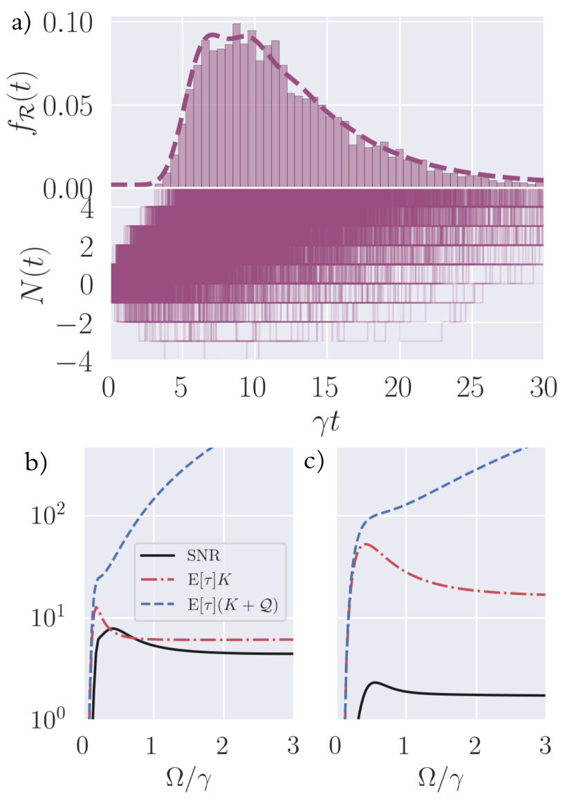
Figure 1: KURs for a driven qubit. a) FPT distribution for $N(t)$ crossing $\mathcal{R}=(-\infty,5]$, with $\Omega=\gamma=1$, $\bar{n}=0.2$ and initial state $\rho_{ss}$. The histogram corresponds to the quantum trajectory simulations, depicted below as a function of time. b,c) SNR (black solid), classical (KUR) Garrahan (2017) (red ‘– $\cdot$’) and quantum KUR Van Vu and Saito (2022) (blue ‘-’) as a function of $\Omega/\gamma$, for $\bar{n}=0.1$ and $1$ respectively. In b) we can see a violation of the classical bound.

We next use this model to study the KURs in Refs. Garrahan (2017); Van Vu and Saito (2022). Formulas for $K$ and $\mathcal{Q}$ are given in Appendix. D. Results comparing the SNR with the two bounds are shown in Fig. 1(b,c) for $\bar{n}=0.1$ and $1$. We see that the classical bound Garrahan (2017) is somewhat tight, and tends to follow the overall behavior of the SNR. However, it can be violated, as in Fig. 1(b). Such quantum violations have been the subject of extensive research Agarwalla and Segal (2018); Ptaszyński (2018); Liu and Segal (2019); Saryal et al. (2019); Cangemi et al. (2020); Kalaee et al. (2021); Prech et al. (2023) as they are connected to dynamical aspects of coherence. Conversely, the quantum bound of Van Vu and Saito (2022) is never violated, as it must. However, it is also rather loose and diverges as $\mathcal{Q}\propto\Omega^{2}$. This result is relevant for the following reason. The classical bound depends only on the dynamical activity $K$ of the observed quantum jumps associated to the operators $L_{k}$. But in quantum coherent problems there is also activity associated to the unitary dynamics (the Rabi oscillations in our case), although this is hidden to the observer. This additional activity is precisely what $\mathcal{Q}$ captures.

Single-qubit threshold detector.—As our second application, we use our framework to model a single qubit functioning as a threshold detector for Rabi pulses. This is motivated by the recent experiment in Ref. Petrovnin et al. (2023). Suppose one wishes to know whether a Rabi pulse $\Omega(t)$ (of unknown shape and duration) was applied to a qubit during some time window $\tau$. The goal is to come up with a “yes/no” protocol, based on a continuous measurement record of the qubit, that yields “yes” (click) if the pulse was applied and “no” (no-click) if it was not. To do that, we continuously monitor the qubit’s population, within the diffusive unravelling, resulting in a stochastic net charge $N(\tau)$ [Eq. (7)]. We then choose the interval $\mathcal{R}=[a,b]$ and associate $N(\tau)\notin\mathcal{R}$ with a click (the pulse was applied), and $N(\tau)\in\mathcal{R}$ with no click (the pulse was not applied). In this way, the threshold detector is cast as a first passage time problem. The goal is to choose $\tau$ and $\mathcal{R}$ in order to maximize the successful detection probability $p_{\rm succ}$ and, at the same time, minimize the probability of false positives $p_{\rm false}$ (when the detector clicks “yes” even though no pulse was applied).

We model this using Eq. (6) with $H(t)=\Omega(t)\sigma_{x}$ and a single jump operator $L=\sqrt{\gamma}\sigma_{z}$. We choose $\nu=\sqrt{\gamma}$ to make $N(\tau)$ in Eq. (7) dimensionless. The shape and structure of $\Omega(t)$ depend on the pulse in question. We assume the system starts in $|\!\!\downarrow\rangle$, so if $\Omega(t)\equiv 0$, it will remain there throughout. Any Rabi pulse will therefore tend to partially excite the qubit, which in turn will change the stochastic properties of the signal $N(\tau)$. For a given $\Omega(t)$, the detection probability is obtained by solving Eq. (8), with initial state $|\psi_{0}\rangle=|\!\!\downarrow\rangle$, and following the same steps delineated before to compute the survival probability $G_{\mathcal{R}}(\tau|\Omega(t),|\!\!\downarrow\rangle)$. The successful detection probability is then $p_{\rm succ}=1-G_{\mathcal{R}}(\tau|\Omega(t),|\!\!\downarrow\rangle)$. Conversely, the false positive probability is $p_{\rm false}=1-G_{\mathcal{R}}(\tau|\Omega(t)\equiv 0,|\!\!\downarrow\rangle)$.

The probability $p_{\rm succ}$ depends on the specifics of $\Omega(t)$. For concreteness and simplicity, we will focus here on a delta-like pulse $\Omega(t)=\Omega_{0}\delta(t)$. The complete analytical solution can be found in Appendix E. The resulting success probability reduces to $p_{\rm succ}=p_{-}+q(p_{+}-p_{-})$ where $q=\langle\sigma_{+}\sigma_{-}\rangle_{0}=\sin^{2}(\Omega_{0})$ is the initial state occupation and $p_{\pm}$, which depend only on $a,b,\gamma\tau$, are the detection probabilities for initial states $|\!\!\uparrow\rangle$ and $|\!\!\downarrow\rangle$, respectively. The false positive probability is $p_{\rm false}=p_{-}$. The goal is to minimize $p_{\rm false}$ and maximize $p_{\rm succ}$. Fig. 2 shows regions in the $(a,b)$ plane representing different bounds on $p_{\rm false/succ}$, for fixed $\gamma\tau=1$ and $q=1$. From this image one can infer that optimal operation occurs for small $b$ and large $|a|$; e.g. $b\sim 1$ and $a\sim-5$. Similar conclusions can be drawn by looking at the mean and variance of the FPT. The mean for the two processes are plotted on the inset of Fig. 2 as a function of $a$, with $b=1$ and $q=1$. For large $|a|$, $E_{\rm false}(\tau)\gg\gamma\tau=1$, so false positives are unlikely to occur for this value of $\gamma\tau$. The inset of Fig. 2 also shows how the maximum standard deviation of the FPT, maximized over all $q$, does not grow significantly with $a$. So not only are false positives unlikely on average, but their fluctuations is also small. These results, combined, corroborate this parameter regime as useful for the operation as a detector. Of course, this analysis pertains only to a toy model and, in reality, several other factors would have to be taken into consideration. Notwithstanding, they serve to illustrate how, through the analytical insights from our framework, one can systematically search for optimal operating regimes.

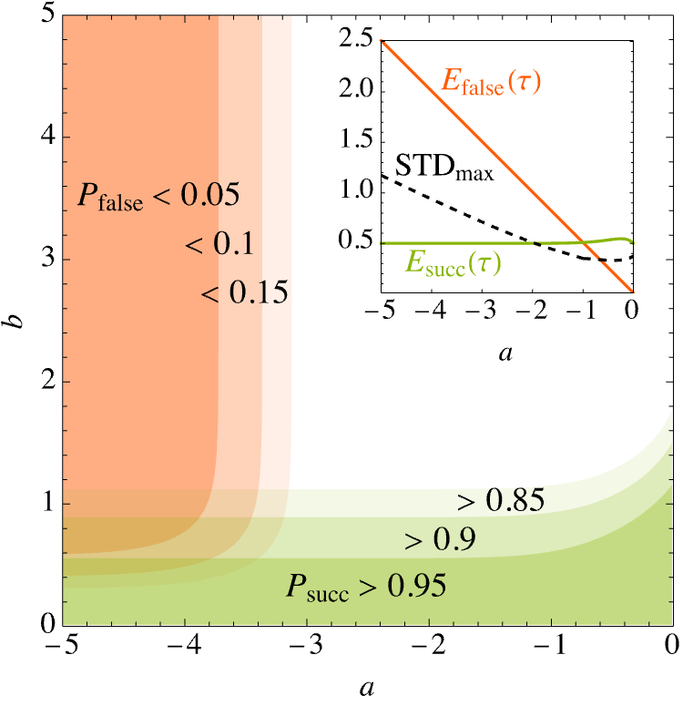
Figure 2: Operation of a continuously monitored qubit as a threshold detector. The plot shows regions in the $(a,b)$ plane with bounds on the false positive detection probability $p_{\rm false}$ and the successful detection probability $p_{\rm succ}$, with fixed $\gamma\tau=1$ and $q=1$ (analytical expressions are shown in Appendix E). The inset shows the average FPT, in units of $\gamma$, for the false positive and the successful detection cases respectively, with $b=1$ and $q=1$. It also shows the maximum possible standard deviation of the FPT, obtained by maximizing over all $q$.

Discussion and conclusions.—Our methodology is compatible with any type of master equation in the form (2), including time-dependent Hamiltonians. It therefore encompass a broad range of physical problems, from quantum optics to condensed matter. In addition, because Eqs. (4) and (8) are resolved in $N$, it is straightforward to extend our method to incorporate $N$-dependent feedback. That is, to study models where $H$ or $\{L_{k}\}$ are modified depending on the current value of $N(t)$ in a quantum trajectory Annby-Andersson et al. (2022). Despite not being the focus of this letter, we emphasize this connection because feedback and FPTs are actually conceptually very similar: both require monitoring of a stochastic quantity and performing (or not) actions depending on its value. In the case of the FPT, the action is to continue or cease the dynamics. In the case of feedback, it is to modify the Liouvillian. Feedback and FPT also share the same practical difficulty of requiring computationally expensive quantum trajectories. Deterministic strategies, such as the one put forth in this letter, are therefore crucial. A famous example of a successful deterministic theory is that of current feedback put forth in Refs. Wiseman and Milburn (1994); Wiseman (1994), which had a significant impact, despite working only for a restricted class of models. We believe a similar point can be made for our results.

A particularly interesting application of our results is to so-called gambling problems, such as that studied in Manzano et al. (2021). This involves an agent which uses information about the system’s state to devise stopping strategies aimed at maximizing a certain goal, which can be relevant in the context of thermodynamics. For instance, depending on the model $N(t)$ can be related to the heat exchanged with the bath, or the work performed by an external drive. An agent with access to either of these quantities could then devise a strategy such as “stop the process whenever a certain amount of work has been extracted.” This has interesting thermodynamic implications, as it puts in the foreground the role of information in thermodynamic processes. It may also have practical consequences. For example, one can use these ideas to devise optimal cooling protocols, or for quantum state engineering.

Acknowledgements– The authors thank Mark Mitchision for the helpful discussions. MJK acknowledges the financial support from a Marie Skłodowska-Curie Fellowship (Grant No. 101065974). SC acknowledges support from the Science Foundation Ireland Starting Investigator Research Grant “SpeedDemon” No. 18/SIRG/5508, the John Templeton Foundation Grant ID 62422, and the Alexander von Humboldt Foundation.

Appendix

Appendix A Derivation of the $N$-resolved master equation

There are multiple ways of deriving an equation for the charge-resolved density matrix. For instance, somewhat similar results have already appeared in Refs. Zoller et al. (1987); Plenio and Knight (1998); Li et al. (2005); Li (2016). These results, however, refer only to quantum jumps. Here we put forth a derivation method that actually applies to any unravelling (hence also including quantum diffusion). Its starting point is the generalized master equation from Full Counting Statistics (FCS). The basic object is the so-called generalized state $\rho_{\chi}(t)$ which is defined in relation to the probability $P(N,t)$ of detecting a charge $N$ at time $t$ according to

$$P(N,t)=\int\limits_{-\infty}^{\infty}\frac{d\chi}{2\pi}e^{-iN\chi}\tr\{\rho_{\chi}(t)\big{\}}.$$ (9)

One can show that $\rho_{\chi}(t)$ satisfies the generalized master equation Esposito et al. (2009); Landi et al. (2022, 2023)

$$\frac{d\rho_{\chi}(t)}{dt}=\mathcal{L}_{\chi}\rho_{\chi}(t),$$ (10)

where $\mathcal{L}_{\chi}$ is the tilted Liouvillian. From Eq. (9) we can define a $N$-resolved density matrix as

$$\rho_{N}(t)=\int\limits_{-\infty}^{\infty}\frac{d\chi}{2\pi}e^{-iN\chi}\rho_{\chi}(t).$$ (11)

We now discretize Eq. (10) in small time-steps $dt$:

$$\rho_{\chi}(t+dt)=\rho_{\chi}(t)+dt\mathcal{L}_{\chi}\rho_{\chi}(t).$$ (12)

Multiplying both sides by $e^{-iN\chi}$, integrating over $\chi$ and substituting $\rho_{\chi}(t)=\int dN^{\prime}e^{iN^{\prime}\chi}\rho_{N^{\prime}}(t)$ we find

$$\rho_{N}(t+dt)=\rho_{N}(t)+dt\int dN^{\prime}\Bigg{[}\int\frac{d\chi}{2\pi}e^{i(N^{\prime}-N)\chi}\mathcal{L}_{\chi}\Bigg{]}\rho_{N^{\prime}}(t).$$ (13)

This is the general form of the $N$-resolved master equation. It relates $\rho_{N}(t+dt)$ to all states $\rho_{N^{\prime}}(t)$ at time $t$. To make it useful, though, we now need to specialize to the jump and diffusion unravelings.

Appendix B Quantum jump unravelling

For quantum jumps the tilted Liouvillian has the form

$$\mathcal{L}_{\chi}\rho=\mathcal{L}_{0}\rho+\sum_{k}e^{i\nu_{k}\chi}L_{k}\rho L_{k}^{\dagger}.$$ (14)

Fourier transforming and using $\int\frac{d\chi}{2\pi}e^{i(N^{\prime}-N+\nu_{k})\chi}=\delta(N^{\prime}-N+\nu_{k})$ reduces Eq. (13) to

$$\rho_{N}(t+dt) =\rho_{N}(t)$$

$$+dt\int dN^{\prime}\delta(N^{\prime}-N)\mathcal{L}_{0}\rho_{N^{\prime}}(t)$$

$$+\sum_{k}\delta(N^{\prime}-N+\nu_{k})L_{k}\rho_{N^{\prime}}(t)L_{k}^{\dagger}$$

$$=\rho_{N}(t)+dt\mathcal{L}_{0}\rho_{N}(t)+dt\sum_{k}L_{k}\rho_{N-\nu_{k}}(t)L_{k}^{\dagger}.$$ (15)

Taking the limit $dt\to 0$ we recover Eq. (4) of the main text. To provide an example of how one can efficiently solve that equation, consider a generic system with two channels, $L_{-}$ and $L_{+}$, and weights $\nu_{-}=1$ and $\nu_{+}=-1$. Eq. (4) then becomes

$$\frac{\partial\rho_{N}}{\partial t}=\mathcal{L}_{0}\rho_{N}+\mathcal{J}_{-}\rho_{N-1}+\mathcal{J}_{+}\rho_{N+1}.$$ (16)

In this case $N(t)$ will take on only integer values. We can solve for all relevant density operators simultaneously, by rewriting this into a single vector equation

$$\frac{d}{dt}\begin{pmatrix}\rho_{a}^{\mathcal{R}}\\ \rho_{a+1}^{\mathcal{R}}\\ \vdots\\ \rho_{b-1}^{\mathcal{R}}\\ \rho_{b}^{\mathcal{R}}\end{pmatrix}=\begin{pmatrix}\mathcal{L}_{0}&\mathcal{J}_{+}&0&\dots&0\\ \mathcal{J}_{-}&\mathcal{L}_{0}&\mathcal{J}_{+}&\dots&0\\ 0&\mathcal{J}_{-}&\ddots&\dots&\vdots\\ \vdots&\vdots&\vdots&\mathcal{L}_{0}&\mathcal{J}_{+}\\ 0&0&\dots&\mathcal{J}_{-}&\mathcal{L}_{0}\end{pmatrix}\begin{pmatrix}\rho_{a}^{\mathcal{R}}\\ \rho_{a+1}^{\mathcal{R}}\\ \vdots\\ \rho_{b-1}^{\mathcal{R}}\\ \rho_{b}^{\mathcal{R}}\end{pmatrix},$$ (17)

where the superscript $\mathcal{R}$ is to emphasize that we are using absorbing boundary conditions, eliminating any $\rho_{N}$ outside of $\mathcal{R}=[a,b]$. As one can see, the result is in the form of a vector-matrix equation $\frac{d\vec{\rho}^{\mathcal{R}}}{dt}=\mathcal{V}\vec{\rho}^{\mathcal{R}}$, whose solution is $\vec{\rho}^{\mathcal{R}}=e^{\mathcal{V}t}\vec{\rho}^{\mathcal{R}}(0)$. The fact that we can write the solution as an exponential map means we do not have to integrate the equation for infinitesimal $dt$, but instead can immediately compute $\vec{\rho}(t)$ at any desired final time.

Appendix C Quantum diffusion unravelling

The tilted Liouvillian for diffusive measurements was derived in Landi et al. (2023) and reads

$$\mathcal{L}_{\chi}=\mathcal{L}+i\chi\sum_{k}\nu_{k}\mathcal{K}[L_{k}]-\frac{\chi^{2}}{2}K_{\rm diff},$$ (18)

where $\mathcal{K}[L]\rho=L\rho+\rho L^{\dagger}$ and $K_{\rm diff}=\sum_{k}\nu_{k}^{2}$. We insert this in Eq. (13). The Fourier transforms now read

$$\int\frac{d\chi}{2\pi}e^{i(N^{\prime}-N)\chi}\chi =-i\frac{\partial}{\partial N^{\prime}}\delta(N^{\prime}-N),$$ (19)

$$\int\frac{d\chi}{2\pi}e^{i(N^{\prime}-N)\chi}\chi^{2} =-\frac{\partial^{2}}{\partial N^{\prime 2}}\delta(N^{\prime}-N).$$ (20)

We therefore find

$$\rho_{N}(t+dt) =\rho_{N}(t)$$

$$+dt\mathcal{L}\rho_{N}(t)dt$$

$$+\int dN^{\prime}\Bigg{[}\frac{\partial}{\partial N^{\prime}}\delta(N^{\prime}-N)\Bigg{]}\sum_{k}\nu_{k}\mathcal{K}[L_{k}]\rho_{N^{\prime}}(t)$$

$$+\frac{dtK_{\rm diff}}{2}\int dN^{\prime}\Bigg{[}\frac{\partial^{2}}{\partial N^{\prime 2}}\delta(N^{\prime}-N)\Bigg{]}\rho_{N^{\prime}}(t).$$ (21)

Finally, we integrate by parts and transfer the derivatives to $\rho_{N^{\prime}}$, leading to

$$\rho_{N}(t+dt) =\rho_{N}(t)+dt\mathcal{L}\rho_{N}(t)$$

$$-dt\sum_{k}\nu_{k}\mathcal{K}[L_{k}]\frac{\partial\rho_{N}(t)}{\partial N}+\frac{K_{\rm diff}dt}{2}\frac{\partial^{2}\rho_{N}(t)}{\partial N^{2}}.$$ (22)

Passing $\rho_{N}(t)$ to the left-hand side, dividing by $dt$ and taking the limit $dt\to 0$ yields

$$\frac{\partial\rho_{N}(t)}{\partial t}=\mathcal{L}\rho_{N}(t)-\sum_{k}\nu_{k}\mathcal{K}[L_{k}]\frac{\partial\rho_{N}(t)}{\partial N}+\frac{K_{\rm diff}}{2}\frac{\partial^{2}\rho_{N}(t)}{\partial N^{2}},$$ (23)

which is the result presented in the main text, Eq. (8).

As far as solving the equation, the methodology is similar to the quantum jumps case. But now $N$ is continuous and therefore must be discretized in small increments $\Delta N$ (an alternative solution method based one expanding in a basis of special functions was introduced in Annby-Andersson et al. (2022), although it is not clear if that is equally applicable here). In terms of finite differences

$$\frac{\partial\rho_{N}}{\partial N} =\frac{\rho_{N+\Delta N}-\rho_{N-\Delta N}}{2\Delta N}$$ (24)

$$\frac{\partial^{2}\rho_{N}}{\partial N^{2}} =\frac{\rho_{N+\Delta N}-2\rho_{N}+\rho_{N-\Delta N}}{(\Delta N)^{2}}\,,$$ (25)

the relevant set of equations become

$$\frac{d}{dt}\left(\begin{array}[]{c}\rho_{a}^{\mathcal{R}}\\ \rho_{a+\Delta N}^{\mathcal{R}}\\ \vdots\\ \rho_{b-\Delta N}^{\mathcal{R}}\\ \rho_{b}^{\mathcal{R}}\end{array}\right)=\left(\begin{array}[]{ccccc}\mathcal{L}-\frac{K_{\rm diff}}{\Delta N^{2}}&-\frac{\mathcal{K}}{2\Delta N}+\frac{K_{\rm diff}}{2\Delta N^{2}}&0&\dots&0\\ \frac{\mathcal{K}}{2\Delta N}+\frac{K_{\rm diff}}{2\Delta N^{2}}&\mathcal{L}-\frac{K_{\rm diff}}{\Delta N^{2}}&-\frac{\mathcal{K}}{2\Delta N}+\frac{K_{\rm diff}}{2\Delta N^{2}}&\dots&0\\ 0&\frac{\mathcal{K}}{2\Delta N}+\frac{K_{\rm diff}}{2\Delta N^{2}}&\ddots&\dots&\vdots\\ \vdots&\vdots&\vdots&\ddots&-\frac{\mathcal{K}}{2\Delta N}+\frac{K_{\rm diff}}{2\Delta N^{2}}\\ 0&0&\dots&\frac{\mathcal{K}}{2\Delta N}+\frac{K_{\rm diff}}{2\Delta N^{2}}&\mathcal{L}-\frac{K_{\rm diff}}{\Delta N^{2}}\end{array}\right)\left(\begin{array}[]{c}\rho_{a}^{\mathcal{R}}\\ \rho_{a+\Delta N}^{\mathcal{R}}\\ \vdots\\ \rho_{b-\Delta N}^{\mathcal{R}}\\ \rho_{b}^{\mathcal{R}}\end{array}\right).$$ (41)

Just like in the jump case, this is in the form of a vector-matrix equation which can easily be solved.

Appendix D Quantum vs Classical KUR

In this section we expand on the KUR’s derived in Garrahan (2017); Van Vu and Saito (2022). The classical bound from Garrahan (2017) reads

$$\frac{{\rm E}[\tau]^{2}}{{\rm Var}[\tau]}\leq{\rm E}[\tau]K\,,$$ (42)

where $K=\sum_{k}\tr(L_{k}^{\dagger}L_{k}\rho_{\rm ss})$ is the steady-state dynamical activity. This bound can be violated in coherent systems. Conversely, the bound derived in Van Vu and Saito (2022), which always holds, reads

$$\frac{{\rm E}[\tau]^{2}}{{\rm Var}[\tau]}\leq{\rm E}[\tau](K+\mathcal{Q})\,,$$ (43)

where

$$\mathcal{Q}=-4\tr\{\mathcal{L}_{1}\mathcal{L}^{+}\mathcal{L}_{2}\rho_{\rm ss}\big{\}}-4\tr\{\mathcal{L}_{2}\mathcal{L}^{+}\mathcal{L}_{1}\rho_{\rm ss}\big{\}}.$$ (44)

Here $\mathcal{L}^{+}$ is the Drazin inverse of the Liouvillian Landi et al. (2023) while

$$\mathcal{L}_{1}\rho =-iH\rho+\frac{1}{2}\sum_{k}\big{(}L_{k}\rho L_{k}^{\dagger}-L_{k}^{\dagger}L_{k}\rho\big{)},$$ (45)

$$\mathcal{L}_{2}\rho =i\rho H+\frac{1}{2}\sum_{k}\big{(}L_{k}\rho L_{k}^{\dagger}-\rho L_{k}^{\dagger}L_{k}\big{)}.$$

For the specific case of the qubit model treated in the main text, we get the following results:

$$K =\frac{2\gamma(2\bar{n}+1)\left[\gamma^{2}\bar{n}(\bar{n}+1)+2\Omega^{2}\right]}{\gamma^{2}(2\bar{n}+1)^{2}+8\Omega^{2}},$$ (46)

$$\mathcal{Q} =\frac{32\Omega^{2}}{\gamma^{2}(2\bar{n}+1)^{2}}K.$$ (47)

Notice how $\mathcal{Q}\to 0$ when $\Omega\to 0$, as this corresponds to the limit where the dynamics becomes incoherent (and hence the two bounds coincide). In the limit of large temperatures we get $K\sim\gamma\bar{n}$, while $\mathcal{Q}\to 0$. Conversely, $\mathcal{Q}/K$ is largest when $\bar{n}\to 0$.

Appendix E Qubit threshold detector model

Here we provide more details on our second example of a qubit functioning as a threshold detector for a Rabi pulse. The system is modeled by the diffusive stochastic master equation (6) with a single jump operator $L=\sqrt{\gamma}\sigma_{z}$ and a time-dependent Hamiltonian $H(t)=\Omega(t)\sigma_{x}$; viz.,

$$d\rho_{c} =-i[\Omega(t)\sigma_{x},\rho_{c}]+\gamma D[\sigma_{z}]\rho_{c}+$$ (48)

$$\qquad\sqrt{\gamma}\Big{(}\sigma_{z}\rho_{c}+\rho_{c}\sigma_{z}-2\langle\sigma_{z}\rangle_{c}\rho_{c}\Big{)}dW(t).$$

The stochastic charge is given by Eq. (7). For convenience we take $\nu=\sqrt{\gamma}$, which makes $N(t)$ dimensionless:

$$N(t)=\int\limits_{0}^{t}dt^{\prime}\Big{[}2\gamma\langle\sigma_{z}\rangle_{c}(t^{\prime})+\sqrt{\gamma}\frac{dW}{dt^{\prime}}\Big{]}.$$ (49)

Our goal is to solve the Quantum Fokker-Planck equation (8) for the charge-resolved density matrix $\rho_{N}(t)$, from which we can then extract the survival and first-passage time probabilities. In what follows, we will use $x$ instead of $N$, and write the charge-resolved density matrix $\rho_{N}(t)$ as $\rho(x,t)$. Eq. (8) then becomes, for this particular problem,

$$\partial_{t}\rho(x,t) =-i\Omega(t)[\sigma_{x},\rho(x,t)]+\gamma D[\sigma_{z}]\rho(x,t)$$ (50)

$$-\gamma\{\sigma_{z},\partial_{x}\rho(x,t)\}+\frac{\gamma}{2}\partial_{x}^{2}\rho(x,t).$$

which is an operator-valued partial differential equation. The operator $\rho(x,t)$ is still Hermitian, but is no longer normalized. We therefore parametrize it as

$$\rho(x,t)=\frac{1}{2}\Big{(}s_{0}(x,t)\sigma_{0}+s_{x}(x,t)\sigma_{x}+s_{y}(x,t)\sigma_{y}+s_{z}(x,t)\sigma_{z}\Big{)},$$ (51)

for new variables $s_{i}(x,t)$, which will satisfy the four coupled partial differential equations

$$\Big{[}\partial_{t}-\frac{\gamma}{2}\partial_{x}^{2}\Big{]}s_{0} =-2\gamma\partial_{x}s_{z},$$ (52)

$$\Big{[}\partial_{t}-\frac{\gamma}{2}\partial_{x}^{2}\Big{]}s_{z} =-2\gamma\partial_{x}s_{0}+2\Omega(t)s_{y},$$ (53)

$$\Big{[}\partial_{t}-\frac{\gamma}{2}\partial_{x}^{2}\Big{]}s_{y} =-2\gamma s_{y}-2\Omega(t)s_{z},$$ (54)

$$\Big{[}\partial_{t}-\frac{\gamma}{2}\partial_{x}^{2}\Big{]}s_{x} =-2\gamma s_{x}.$$ (55)

Upon solving this we obtain our desired probability as $P_{\mathcal{R}}(x,t)=\tr\{\rho(x,t)\big{\}}=s_{0}(x,t)$ (with $x\equiv N$). Notice how $s_{x}(x,t)$ is decoupled from $s_{0},s_{z},s_{y}$. Hence, effectively we only need to solve 3 coupled partial differential equations (52)-(54). These are subject to the initial conditions $\rho(x,0)=\rho(0)\delta(x-x_{0})$, where $\rho(0)$ is the initial state and $x_{0}$ is the initial value of the charge, $x_{0}\equiv N(0)$. Throughout the main text we have assumed that this always started at $x_{0}=0$. However, we will see below that it is advantageous to keep it general.

Define the 3-component vector $\xi(x,t)=\big{(}s_{0}(x,t),s_{z}(x,t),s_{y}(x,t)\big{)}$. Eqs. (52)-(54) can then be written more compactly as

$$\Big{[}\partial_{t}-\frac{\gamma}{2}\partial_{x}^{2}+2\gamma M_{1}\partial_{x}+M_{2}\Big{]}\xi=0,$$ (56)

where

$$M_{1}=\begin{pmatrix}0&1&0\\ 1&0&0\\ 0&0&0\end{pmatrix},\qquad M_{2}=\begin{pmatrix}0&0&0\\ 0&0&-2\Omega(t)\\ 0&2\Omega(t)&2\gamma\end{pmatrix}.$$ (57)

We now transform to a new variable $\mu(x,t)$ according to $\xi(x,t)=e^{2xM_{1}}\mu(x,t)$. This modifies Eq. (56) to

$$\Big{[}\partial_{t}-\frac{\gamma}{2}\partial_{x}^{2}+2\gamma-2\Omega(t)M_{3}(x)\Big{]}\mu(x,t)=0,$$ (58)

where

$$M_{3}(x)=\left(\begin{array}[]{ccc}0&0&-\sinh(2x)\\ 0&0&\cosh(2x)\\ -\sinh(2x)&-\cosh(2x)&0\\ \end{array}\right).$$ (59)

The Rabi drive therefore make the equations inhomogeneous in $x$.

E.1 Solution for delta-like pulse

We specialize the above calculations to the case of a delta-like pulse $\Omega(t)=\Omega_{0}\delta(t)$. Initially the qubit is in the spin down state $|\!\!\downarrow\rangle$. The delta pulse will push it to $|\psi_{0}\rangle=-i\sin(\Omega_{0})|\!\!\uparrow\rangle+\cos(\Omega_{0})|\!\!\downarrow\rangle$. For $t=0^{+}$, the system will then evolve as if $\Omega(t)=0$. Recall we must employ absorbing boundary conditions on an interval $\mathcal{R}=[a,b]$. We will first focus on a solution for the interval $\mathcal{R}=[0,b]$. Afterwards, we will then shift the solution so that it encompass a generic interval $\mathcal{R}=[a,b]$. When $\Omega(t)=0$ the entries of $\mu(x,t)$ decouple in Eq. (58), each satisfying an identical equation, which is nothing but a scalar diffusion equation with a constant shift and also subject to absorbing boundaries at the endpoints. The solution, as one can verify, is

$$\mu(x,t)=\sqrt{\frac{2}{b}}\sum_{n=1}^{\infty}e^{-\gamma t(2+k_{n}^{2}/2)}a_{n}\sin(k_{n}x),$$ (60)

where $k_{n}=\frac{\pi n}{b}$ and $a_{n}$ is a 3-component vector of constants that are fixed by the initial conditions. Returning to the original variable $\xi(x,t)=e^{2xM_{1}}\mu(x,t)$ we get

$$\xi(x,t)=\sqrt{\frac{2}{b}}\sum_{n=1}^{\infty}e^{-\gamma t(2+k_{n}^{2}/2)}e^{2xM_{1}}a_{n}\sin(k_{n}x).$$ (61)

The initial conditions is $\xi(x,0)=\delta(x-x_{0})\xi_{0}$ where $\xi_{0}=(1,\langle\sigma_{z}\rangle_{0},\langle\sigma_{y}\rangle_{0})$ and $\langle\ldots\rangle_{0}=\langle\psi_{0}|\ldots|\psi_{0}\rangle$. Using the orthogonality of the Fourier coefficients we find

$$a_{n}=\sqrt{\frac{2}{b}}\sin(k_{n}x_{0})e^{-2x_{0}M_{1}}\xi_{0}.$$ (62)

Hence, the final solution reads

$$\xi(x,t)=\frac{2}{b}\sum_{n=1}^{\infty}e^{-\gamma t(2+k_{n}^{2}/2)}\sin(k_{n}x)\sin(k_{n}x_{0})e^{2(x-x_{0})M_{1}}\xi_{0}.$$ (63)

The quantity we are interested in is $P(x,t)=s_{0}(x,t)$, which is the first component of $\xi(x,t)$. Hence

$$P_{[0,b]}(x,t) =\frac{2}{b}\sum_{n=1}^{\infty}e^{-\gamma t(2+k_{n}^{2}/2)}\sin(k_{n}x)\sin(k_{n}x_{0})$$ (64)

$$\times\bigg{(}\cosh(2x-2x_{0})+\langle\sigma_{z}\rangle_{0}\sinh(2x-2x_{0})\bigg{)}.$$

Notice how the result is independent of $\langle\sigma_{y}\rangle_{0}$.

This solution holds for an interval $\mathcal{R}=[0,b]$. To obtain the general solution for arbitrary interval we shift all variables $x\to x-a$, $x_{0}\to x_{0}-a$ and $b\to b-a$. This yields

$$P_{\mathcal{R}}(x,t) =C\sum_{n=1}^{\infty}e^{-\gamma t(2+k_{n}^{2}/2)}\sin(k_{n}(x-a))\sin(k_{n}(x_{0}-a))$$ (65)

$$\times\bigg{(}\cosh(2x-2x_{0})+\langle\sigma_{z}\rangle_{0}\sinh(2x-2x_{0})\bigg{)},$$

where, now, $k_{n}=\frac{n\pi}{b-a}$ and we defined $C=\frac{2}{b-a}$. It is more convenient to work with the qubit occupation $\langle\sigma_{z}\rangle=2q-1$, where $q=\langle\sigma_{+}\sigma_{-}\rangle_{0}=\sin^{2}(\Omega_{0})$. We then obtain

$$P_{\mathcal{R}}(x,t)=P_{-}(x,t)+q\big{[}P_{+}(x,t)-P_{-}(x,t)\big{]},$$ (66)

where

$$P_{\pm}(x,t)=Ce^{\pm 2(x-x_{0})}\sum_{n=1}^{\infty}e^{-\gamma t(2+k_{n}^{2}/2)}\sin(k_{n}(x-a))\sin(k_{n}(x_{0}-a)).$$ (67)

These are the probabilities given that initially the qubit was fully polarized up or down. The way they are written, they are not very symmetric when it comes to the interval $\mathcal{R}=[a,b]$. One can verify however, that if we replace $x\to-x$, $a\to-b$ and $b\to-a$ in $P_{-}$ we obtain $P_{+}$ (and vice-versa). This allows us to write a more symmetric version by replacing $P_{+}(x,t;a,b)$ with $[P_{+}(x,t;a,b)+P_{-}(-x,t,-b,-a)]/2$ (and similarly for $P_{-}$). We then get

$$P_{\pm}(x,t) =Ce^{\pm 2x}\sum_{n=1}^{\infty}e^{-\gamma t(2+k_{n}^{2}/2)}\Big{\{}2\cos(k_{n}x)$$ (68)

$$-\cos[k_{n}(x-2a)]-\cos[k_{n}(x-2b)]\Big{\}},$$

which is now more symmetrical in $a$ and $b$. For simplicity, we have also set $x_{0}=0$ here, to simplify the formula. Eqs. (66) and (68) are the final result. They give the probability of finding the system with a charge $N(t)=x$ at time $t$ for any initial state $\rho_{0}$.

E.2 Survival probability and first passage time

The survival probability $G_{\mathcal{R}}(t)=\int_{a}^{b}dx±P_{\mathcal{R}}(x,t)$ similarly decomposes as

$$G_{\mathcal{R}}(t)=G_{-}(t)+q\big{[}G_{+}(t)-G_{-}(t)\big{]},$$ (69)

where

$$G_{\pm}(t)=C\sum_{n=1}^{\infty}\frac{k_{n}}{4+k_{n}^{2}}e^{-\gamma t(2+k_{n}^{2}/2)}\big{[}e^{\pm 2b}\sin(k_{n}b)-e^{\pm 2a}\sin(k_{n}a)\big{]}.$$ (70)

The detection probabilities $p_{\pm}$ used in the main text are $p_{\pm}=1-G_{\pm}$. And, recall, $p_{\rm false}=p_{-}$ while $p_{\rm succ}=p_{-}+q(p_{+}-p_{-})$.

The first passage time $f_{\mathcal{R}}=-\frac{dG_{\mathcal{R}}}{dt}$ also decomposes in the same way, $f_{\mathcal{R}}(t)=f_{-}(t)+q\big{[}f_{+}(t)-f_{-}(t)\big{]}$, with

$$f_{\pm}(t)=\frac{C}{2}\sum_{n=1}^{\infty}\gamma k_{n}e^{-\gamma t(2+k_{n}^{2}/2)}\big{[}e^{\pm 2b}\sin(k_{n}b)-e^{\pm 2a}\sin(k_{n}a)\big{]}.$$ (71)

From this we get the average first passage time

$$E_{\pm}(\tau)=\frac{C}{2\gamma}\sum_{n=1}^{\infty}\frac{4k_{n}}{(4+k_{n}^{2})^{2}}\big{[}e^{\pm 2b}\sin(k_{n}b)-e^{\pm 2a}\sin(k_{n}a)\big{]}.$$ (72)

If $a,b$ are not too small, we can convert the sum to an integral yielding

$$E_{\pm}(\tau)=\frac{1}{\pi\gamma}\int_{0}^{\infty}dk\frac{4k}{(4+k^{2})^{2}}\big{[}e^{\pm 2b}\sin(kb)-e^{\pm 2a}\sin(ka)\big{]}.$$ (73)

Carrying out the integration yields the approximate formulas

$$E_{-}(\tau)=\frac{1}{2\gamma}\big{(}be^{-4b}+|a|),\qquad E_{+}(\tau)=\frac{1}{2\gamma}\big{(}b+|a|e^{-4|a|}).$$ (74)

Lastly, we study the variance of the FPT. The second moment follows readily from (71):

$$E_{\pm}(\tau^{2})=\frac{C}{2\gamma^{2}}\sum_{n=1}^{\infty}\frac{16k_{n}}{(4+k_{n}^{2})^{3}}\big{[}e^{\pm 2b}\sin(k_{n}b)-e^{\pm 2a}\sin(k_{n}a)\big{]}.$$ (75)

Unlike the moments, the variance of the FPT is not linear in $q$. Instead, from the law of total variance we have that

$${\rm var}(\tau)=(1-q){\rm var}_{-}(\tau)+q{\rm var}_{+}(\tau)+q(1-q)\big{[}E_{+}(\tau)-E_{-}(\tau)\big{]}^{2}.$$ (76)

where ${\rm var}_{\pm}(\tau)=E_{\pm}(\tau^{2})-[E_{\pm}(\tau)]^{2}$ (and hence can be computed using (72) and (75)). Unless $q\equiv 0$ or $q\equiv 1$, the variance will therefore also depend on the average FPTs. The quantity plotted as a black dashed line on the inset of Fig. 2 is the standard deviation $\sqrt{{\rm var}(\tau)}$ maximized over all possible values of $q\in[0,1]$.

References

- Gillespie (1991) D. T. Gillespie, Markov processes: an introduction for physical scientists (Elsevier, 1991).
- Gardiner et al. (1985) C. W. Gardiner et al., Handbook of stochastic methods, Vol. 3 (springer Berlin, 1985).
- Manzano et al. (2021) G. Manzano, D. Subero, O. Maillet, R. Fazio, J. P. Pekola, and E. Roldán, Phys. Rev. Lett. 126, 080603 (2021).
- Sathyamoorthy et al. (2016) S. R. Sathyamoorthy, T. M. Stace, and G. Johansson, Comptes Rendus Physique 17, 756 (2016), quantum microwaves / Micro-ondes quantiques.
- Petrovnin et al. (2023) K. Petrovnin, J. Wang, M. Perelshtein, P. Hakonen, and G. S. Paraoanu, (2023), arXiv:2308.07084v1 [quant-ph] .
- Irwin and Hilton (2005) K. Irwin and G. Hilton, “Transition-edge sensors,” in Cryogenic Particle Detection (Springer Berlin Heidelberg, 2005) p. 63–150.
- Roldán et al. (2015) E. Roldán, I. Neri, M. Dörpinghaus, H. Meyr, and F. Jülicher, Phys. Rev. Lett. 115, 250602 (2015).
- Neri (2020) I. Neri, Phys. Rev. Lett. 124, 040601 (2020).
- Ptaszyński (2018) K. Ptaszyński, Phys. Rev. E 97, 012127 (2018).
- Saito and Dhar (2016) K. Saito and A. Dhar, EPL (Europhysics Letters) 114, 50004 (2016).
- Neri et al. (2017) I. Neri, E. Roldán, and F. Jülicher, Phys. Rev. X 7, 011019 (2017).
- Garrahan (2017) J. P. Garrahan, Phys. Rev. E 95, 032134 (2017).
- Gingrich and Horowitz (2017) T. R. Gingrich and J. M. Horowitz, Phys. Rev. Lett. 119, 170601 (2017).
- Manzano et al. (2019) G. Manzano, R. Fazio, and E. Roldán, Phys. Rev. Lett. 122, 220602 (2019).
- Falasco and Esposito (2020) G. Falasco and M. Esposito, Phys. Rev. Lett. 125, 120604 (2020).
- Pal et al. (2021) A. Pal, S. Reuveni, and S. Rahav, Phys. Rev. Res. 3, L032034 (2021).
- Van Vu and Saito (2022) T. Van Vu and K. Saito, Phys. Rev. Lett. 128, 140602 (2022).
- He et al. (2022) X. He, P. Pakkiam, A. A. Gangat, M. J. Kewming, G. J. Milburn, and A. Fedorov, arXiv preprint arXiv:2207.11043 (2022).
- Singh et al. (2019) S. Singh, P. Menczel, D. S. Golubev, I. M. Khaymovich, J. T. Peltonen, C. Flindt, K. Saito, E. Roldán, and J. P. Pekola, Phys. Rev. Lett. 122, 230602 (2019).
- Carmichael et al. (1989) H. J. Carmichael, S. Singh, R. Vyas, and P. R. Rice, Phys. Rev. A 39, 1200 (1989).
- Plenio and Knight (1998) M. B. Plenio and P. L. Knight, Reviews of Modern Physics 70, 101–144 (1998).
- Wiseman and Milburn (2009) H. M. Wiseman and G. J. Milburn, Quantum measurement and control (Cambridge university press, 2009).
- Landi et al. (2023) G. T. Landi, M. J. Kewming, M. T. Mitchison, and P. P. Potts, (2023), arXiv:2303.04270v2 [quant-ph] .
- Stratonovich (1963) R. L. Stratonovich, Topics in the theory of random noise, Vol. 1 (Gordon and Breach, Science Publishers, Inc., 1963).
- Vyas and Singh (1988) R. Vyas and S. Singh, Phys. Rev. A 38, 2423 (1988).
- Brandes (2008) T. Brandes, Ann. Phys. 17, 477 (2008).
- Thomas and Flindt (2013) K. H. Thomas and C. Flindt, Phys. Rev. B 87, 121405 (2013).
- Haack et al. (2014) G. Haack, M. Albert, and C. Flindt, Phys. Rev. B 90, 205429 (2014).
- Skinner and Dunkel (2021) D. J. Skinner and J. Dunkel, Phys. Rev. Lett. 127, 198101 (2021).
- Schulz et al. (2022) F. Schulz, D. Chevallier, and M. Albert, (2022), arXiv:2210.01080 [cond-mat.mes-hall] .
- Brandes and Emary (2016) T. Brandes and C. Emary, Physical Review E 93, 042103 (2016), arxiv:1602.02975 .
- Kosov (2016) D. S. Kosov, “Distribution of waiting times between superoperator quantum jumps in Lindblad dynamics,” (2016), arxiv:1605.02170 [cond-mat, physics:quant-ph] .
- Ptaszyński (2017) K. Ptaszyński, Physical Review B 96, 035409 (2017), arxiv:1707.00441v1 .
- Kleinherbers et al. (2021) E. Kleinherbers, P. Stegmann, and J. König, Physical Review B 104, 165304 (2021), arxiv:2107.10218 .
- Albert et al. (2011) M. Albert, C. Flindt, and M. Büttiker, Physical Review Letters 107, 086805 (2011), arxiv:1102.4452 .
- Stefanov et al. (2022) V. Stefanov, V. Shatokhin, D. Mogilevtsev, and S. Kilin, Physical Review Letters 129 (2022), 10.1103/physrevlett.129.083603.
- Bolund and Mølmer (2014) A. Bolund and K. Mølmer, Phys. Rev. A 89, 023827 (2014).
- Korotkov and Jordan (2006) A. N. Korotkov and A. N. Jordan, Physical Review Letters 97 (2006), 10.1103/physrevlett.97.166805.
- Zoller et al. (1987) P. Zoller, M. Marte, and D. F. Walls, Phys. Rev. A 35, 198 (1987).
- Li et al. (2005) X.-Q. Li, P. Cui, and Y. Yan, Phys. Rev. Lett. 94, 066803 (2005).
- Li (2016) X.-Q. Li, Frontiers of Physics 11 (2016), 10.1007/s11467-016-0539-8.
- Landi et al. (2022) G. T. Landi, D. Poletti, and G. Schaller, Reviews of Modern Physics 94 (2022), 10.1103/revmodphys.94.045006.
- Schaller (2014) G. Schaller, Open Quantum Systems Far from Equilibrium (2014).
- Esposito et al. (2009) M. Esposito, U. Harbola, and S. Mukamel, Reviews of Modern Physics 81, 1665 (2009).
- Levitov and Lesovik (1993) L. Levitov and G. Lesovik, JETP letters 58, 230 (1993).
- Levitov et al. (1996) L. S. Levitov, H. Lee, and G. B. Lesovik, Journal of Mathematical Physics 37, 4845 (1996).
- Nazarov and Kindermann (2003) Y. V. Nazarov and M. Kindermann, The European Physical Journal B - Condensed Matter and Complex Systems 35, 413 (2003).
- Flindt et al. (2010) C. Flindt, T. Novotný, A. Braggio, and A.-P. Jauho, Physical Review B 82, 155407 (2010), arxiv:1002.4506 .
- Karimi and Pekola (2020) B. Karimi and J. P. Pekola, Physical Review Letters 124 (2020), 10.1103/physrevlett.124.170601.
- K. Murch and Siddiqi (2013) C. M. K. Murch, S. Weber and I. Siddiqi, Nature 502, 211 (2013).
- Campagne-Ibarcq et al. (2016) P. Campagne-Ibarcq, P. Six, L. Bretheau, A. Sarlette, M. Mirrahimi, P. Rouchon, and B. Huard, Physical Review X 6 (2016), 10.1103/physrevx.6.011002.
- Didier et al. (2015) N. Didier, J. Bourassa, and A. Blais, Phys. Rev. Lett. 115, 203601 (2015).
- Blais et al. (2021) A. Blais, A. L. Grimsmo, S. M. Girvin, and A. Wallraff, Rev. Mod. Phys. 93, 025005 (2021).
- Naghiloo et al. (2020) M. Naghiloo, D. Tan, P. Harrington, J. Alonso, E. Lutz, A. Romito, and K. Murch, Physical Review Letters 124 (2020), 10.1103/physrevlett.124.110604.
- Hofmann et al. (2016) A. Hofmann, V. Maisi, C. Gold, T. Krähenmann, C. Rössler, J. Basset, P. Märki, C. Reichl, W. Wegscheider, K. Ensslin, and T. Ihn, Physical Review Letters 117 (2016), 10.1103/physrevlett.117.206803.
- Note (1) As a consistency check, note how , as expected.
- Note (2) Notice that if and , we recover the standard FCS distribution .
- Annby-Andersson et al. (2022) B. Annby-Andersson, F. Bakhshinezhad, D. Bhattacharyya, G. D. Sousa, C. Jarzynski, P. Samuelsson, and P. P. Potts, Physical Review Letters 129 (2022), 10.1103/physrevlett.129.050401.
- Erker et al. (2017) P. Erker, M. T. Mitchison, R. Silva, M. P. Woods, N. Brunner, and M. Huber, Physical Review X 7 (2017), 10.1103/physrevx.7.031022.
- Agarwalla and Segal (2018) B. K. Agarwalla and D. Segal, Physical Review B 98 (2018), 10.1103/physrevb.98.155438.
- Ptaszyński (2018) K. Ptaszyński, Physical Review B 98 (2018), 10.1103/physrevb.98.085425.
- Liu and Segal (2019) J. Liu and D. Segal, Physical Review E 99 (2019), 10.1103/physreve.99.062141.
- Saryal et al. (2019) S. Saryal, H. M. Friedman, D. Segal, and B. K. Agarwalla, Physical Review E 100 (2019), 10.1103/physreve.100.042101.
- Cangemi et al. (2020) L. M. Cangemi, V. Cataudella, G. Benenti, M. Sassetti, and G. D. Filippis, Physical Review B 102 (2020), 10.1103/physrevb.102.165418.
- Kalaee et al. (2021) A. A. S. Kalaee, A. Wacker, and P. P. Potts, Physical Review E 104 (2021), 10.1103/physreve.104.l012103.
- Prech et al. (2023) K. Prech, P. Johansson, E. Nyholm, G. T. Landi, C. Verdozzi, P. Samuelsson, and P. P. Potts, Physical Review Research 5 (2023), 10.1103/physrevresearch.5.023155.
- Wiseman and Milburn (1994) H. M. Wiseman and G. J. Milburn, Physical Review Letters 72, 4054 (1994).
- Wiseman (1994) H. M. Wiseman, Physical Review A 50, 4428 (1994).