Misspecified Bernstein-Von Mises theorem for hierarchical models

Abstract

We derive a Bernstein von-Mises theorem in the context of misspecified, non-i.i.d., hierarchical models parametrized by a finite-dimensional parameter of interest. We apply our results to hierarchical models containing non-linear operators, including the squared integral operator, and PDE-constrained inverse problems. More specifically, we consider the elliptic, time-independent Schrödinger equation with parametric boundary condition and general parabolic PDEs with parametric potential and boundary constraints. Our theoretical results are complemented with numerical analysis on synthetic data sets, considering both the square integral operator and the Schrödinger equation.

1 Introduction

Hierarchical models are frequently used in various fields, for instance in astronomy (weak lensing Alsing et al. (2016); Sellentin, Heymans and Harnois-Déraps (2018), cosmic microwave background (CMB) temperature maps Eriksen et al. (2004), gravitational waves Cornish and Littenberg (2015)), in statistical physics (the Dyson hierarchical model Monthus and Garel (2011)), in environmental sciences (predicting the spread of ecological processes Wikle (2003)) and in medicine (spatial modelling of fMRI data Bowman et al. (2008)). Hierarchical models specify a data-generating process in multiple layers, which yields great modelling flexibility. The connections between the layers are often non-linear, governed by some (system of) partial differential equations. This complex structure imposes analytical and computational challenges.

The goal is to make inference on aspects of the hierarchical process. The direct application of exact methods for inference is typically computationally overly expensive or even infeasible. Therefore, in practice often a surrogate, approximate likelihood is considered instead of the likelihood of the multilayer data-generating structure. For computational convenience and easy interpretation, misspecified Gaussian likelihoods are popular. However, using the simplified likelihood results in information loss and may lead to inaccurate error bands. Although in practice one is aware of the inaccuracy of the misspecified hierarchical procedures, these are typically used without rigorous theoretical guarantees or understanding of their limitations. This sometimes results in contradictory results.

This article was motivated by a concrete example from astronomy. Cosmic microwave background radiation (a snapshot of the universe approximately $3*10^{5}$ years after the big bang) is modelled as a draw from a Gaussian random field (although the Gaussianity is debated Marinucci (2004)). In our current time, we observe non-linear transformations of this field, which can be described by systems of complex partial differential equations, corrupted with noise. Due to the non-linearity, the observed data are non-Gaussian. The goal is to recover important, parametric aspects of the non-linear operators (and their surrogates). This includes the proportion of dark energy and dark matter, and the Hubble constant (the relative expansion rate of the universe). The article Ezquiaga and Zumalacárregui (2018) reviews tools for understanding the nature of dark energy using gravitational waves. To simplify the model and the computations, the complex hierarchical model is replaced by a Gaussian approximation. Figure 8 of Ezquiaga and Zumalacárregui (2018) collects the outcome of a collection of methods for estimating the Hubble constant. One can observe that the resulting error bars of the proposed estimators do not intersect, providing contradictory conclusions about the relative expansion rate of the universe. Understanding the theoretical properties of such, misspecified, hierarchical approaches is important to know whether the non-overlapping confidence intervals are due to using different models or due to statistical error. Here we consider such a result in a misspecified Gaussian framework.

In this article, we consider Bayesian methods for inference on parametric aspects of the complex, hierarchical data-generating process. Bayesian methods have gained popularity in many fields, due to their built-in uncertainty quantification and their ability to provide a natural way of incorporating preliminary knowledge into the observational model. In our work, we focus on the theoretical, asymptotic properties of the posterior distribution on the parameter of interest and investigate whether it can achieve optimal recovery and reliable uncertainty quantification. In regular, parametric models this is done typically by deriving a Bernstein-von Mises result, which assures that the posterior distribution is asymptotically Gaussian, centred at an efficient estimator and with variance equal to the Cramér-Rao bound.

We consider a general misspecified model indexed by finite-dimensional parameters and derive a Bernstein-von Mises theorem, giving a Gaussian approximation of the posterior distribution. Bernstein-von Mises type results have been derived in the literature for various models, starting from well-specified regular parametric models Doob (1949); Le Cam (2012); van der Vaart (1998), and extended to misspecified models; see Kleijn and van der Vaart (2012) and the recent review article Bochkina (2022). Extensions to semi-parametric Castillo and Rousseau (2015) and non-parametric models for weak norms were considered in Haralambie (2011); Castillo and Nickl (2014), while recently a more accurate, skewed version of the theorem was derived in Durante, Pozza and Szabó (2023). However, none of these results consider hierarchical models as examples, and the derived misspecified results depend on conditions that are not met by our highly non-linear examples. Thus, first, we derive a new, modified version of the classical misspecified theorem. Next, we apply this to a collection of hierarchical models, starting with the square integral operator as a toy example and next turning to partial differential equation (PDE) constrained inverse problems. We first investigate the time-independent Schrödinger equation, which allows tractable computations and is often used as a platform for investigating more complex PDE-constrained inverse problems. Then we derive asymptotic guarantees for general parabolic PDEs with parametric potential and boundary constraints. We consider observations at different time points, mimicking typical non-i.i.d. observational structures from physics and astronomy.

The article is organized as follows. In Section 2 we introduce the hierarchical observational model, its Gaussian surrogate and the misspecified Bayesian framework. In Section 3 we provide our general misspecified Bernstein-von Mises theorem and in Section 3.2 we apply it to hierarchical models. Our main contribution is to cover several interesting, PDE-constrained inverse problems, and is presented in Section 4. In Section 5 we investigate the numerical behaviour of our limiting misspecified posterior in contrast to the well-specified case and the accuracy of the Gaussian approximation. The proofs of the general results, examples, and additional technical lemmas are deferred to Sections 6, 7, 8, and 9.

2 Description of the problem

We consider non-linear hierarchical models of the form

$$f_{i} \stackrel{{\scriptstyle\text{i.i.d.}}}{{\sim}}G,\qquad\qquad i=1,\ldots,N,$$ (1)

$$X_{i}\mid f_{i},\theta_{0} \stackrel{{\scriptstyle\text{ind}}}{{\sim}}N_{p}(T_{\theta_{0}}^{(i)}f_{i},\Lambda^{(i)}),\qquad i=1,\ldots,N.$$

Here $G$ is a distribution on some Hilbert space $(\mathcal{F},\langle\cdot,\cdot\rangle_{\mathcal{F}})$, $T_{\theta}^{(i)}:\mathcal{F}\mapsto\mathbb{R}^{p}$ are (possibly) non-linear operators, indexed by an unknown finite-dimensional parameter $\theta\in\mathbb{R}^{d}$ of interest, and $\Lambda^{(i)}\in\mathbb{R}^{p\times p}$ are known, positive-definite covariance matrices. We denote the distribution of $X_{i}$ by $P_{\theta,i}$, for $i=1,\ldots,N$, assume that this has a density $p_{\theta,i}$ relative to some measure $\lambda$, and denote the expectation and covariance matrix with respect to this distribution by, for $i=1,\ldots,N$,

$$\mu_{\theta}^{(i)}:=\mathbb{E}_{\theta,i}X_{i},\qquad\qquad\Sigma_{\theta}^{(i)}:=\mathop{\mathrm{Cov}}\nolimits_{\theta,i}(X_{i}).$$ (2)

We aim at making inference on the unknown model parameter $\theta_{0}\in\Theta\subset\mathbb{R}^{d}$ of interest. In case the operators $T_{\theta_{0}}^{(i)}$ are the same for all $i=1,\ldots,N$, we arrive at an i.i.d. model for $(X_{i})_{i=1,\ldots,N}$.

The first layer in (1) models a random non-parametric functional parameter $f_{i}$. The second layer describes the actual observations, which depend on some (possibly) non-linear transformation of the functional parameter, and are corrupted with Gaussian noise. In Section 4 we consider several specific examples of this form, including elliptic and parabolic PDE-constrained inverse problems. The goal is to recover the unknown parameter $\theta_{0}$ of the hierarchical model (1). In applications the operators $T_{\theta}^{(i)}$ can be complex (see the examples in the introduction), but the main goal is typically the same: to recover certain parametric aspects of the model/operator.

In practice simplified, approximate models are used to speed up computations and increase the interpretability of the model. In particular, it is common to replace the otherwise complex likelihood with a Gaussian approximation with mean and covariance matching the corresponding quantities in the original model. In our analysis, we consider the misspecified model $Q_{\theta,i}=N_{p}(\mu_{\theta}^{(i)},\Sigma_{\theta}^{(i)})$ for $X_{i}$, for $i=1,\ldots,N$, with corresponding likelihood $q_{\theta,i}$. Using a misspecified model naturally results in information loss and requires care with uncertainty quantification. We investigate the accuracy of inference on $\theta_{0}$ using this Gaussian, misspecified model, and quantify the amount of information loss and the uncertainty of the procedure.

In our analysis we consider a Bayesian approach and investigate its frequentist properties. We endow the parameter $\theta\in\mathbb{R}^{d}$ in the misspecified likelihood $q_{\theta,i}$ with a prior distribution $\Pi$ with a density $\pi$ satisfying standard regularity assumptions, to be specified later. We then investigate the asymptotic behaviour of the misspecified posterior distribution for $\theta$, i.e. the random measure

$$\Pi(\theta\in A|X_{1},\ldots,X_{N})=\frac{\int_{A}\prod_{i=1}^{N}q_{\theta,i}(X_{i})\pi(\theta)\,d\theta}{\int_{\Theta}\prod_{i=1}^{N}q_{\theta,i}(X_{i})\pi(\theta)\,d\theta},$$ (3)

for Borel sets $A\subset\Theta$. We derive a Bernstein-von Mises type result in this misspecified model, which shows that asymptotically this random measure converges to a Gaussian distribution. Under mild assumptions this contracts around the parameter $\theta_{N}^{*}\in\Theta$ minimizing the Kullback-Leibler divergence between the misspecified Gaussian class and the original model, i.e.

$$\theta_{N}^{*}=\mathop{\rm argmin}_{\theta\in\Theta}P_{\theta_{0}}^{(N)}\biggl{(}\sum_{i=1}^{N}\log\frac{p_{\theta_{0},i}(X_{i})}{q_{\theta,i}(X_{i})}\biggr{)}.$$

We show that in our setup $\theta_{N}^{*}$ coincides with the parameter of interest $\theta_{0}$, and derive the covariance matrix of the limiting Gaussian distribution. We investigate how this differs from the well-specified posterior distribution, both theoretically and numerically for various synthetic data sets.

3 Misspecified Bernstein-von Mises Theorem

The asymptotic behaviour of the posterior distribution in regular parametric models is characterized by the celebrated Bernstein-von Mises theorem. However, in practice often simplified models are considered, to speed up computations and improve the interpretation. In such cases, we talk about misspecified models. As an example, in the previous section we have introduced the complex hierarchical model (1), and we use a surrogate Gaussian model $q_{\theta,i}$. In this section, we first derive a Bernstein-von Mises theorem for misspecified models that goes beyond our hierarchical model (1) and next apply it to the latter special case.

3.1 A general Bernstein-von Mises theorem

Misspecified Bernstein-von Mises results were derived in the literature before, see for instance Kleijn and van der Vaart (2012), but under conditions too strong for our situation. In particular, to obtain a $\sqrt{N}$-contraction rate, the paper Kleijn and van der Vaart (2012) assumes that the log misspecified likelihood is locally Lipschitz with a majorizing function that has exponential moments, which is violated for examples of our model (1), as demonstrated in Remark 1 in Section 4 below. In this section, we present a theorem that is appropriate for the model (1), and applies to hierarchical observational models with a selection of non-linear operators $T_{\theta,i}$.

The conditions of the theorem are essentially the classical ones given in Theorem 7.1 in Lehmann (1983) (given there for the well-specified case, i.i.d. data and a one-dimensional parameter), but are at a high enough level of abstraction that they apply to general models, also beyond independent observations.

Let $l^{(N)}(\theta)$ and $\nabla l^{(N)}(\theta)$ denote a possibly misspecified log-likelihood and its gradient, of a model for an observation $X_{N}$. Given $\theta_{N}^{*}\in\mathbb{R}^{d}$ and symmetric nonnegative-definite $d\times d$ matrices $V_{\theta_{N}^{*},N}$, define, for $\theta\in\Theta$, symmetric matrices $R_{N}(\theta)$ through

$$l^{(N)}(\theta) =l^{(N)}(\theta_{N}^{*})+\nabla l^{(N)}(\theta_{N}^{*})^{\intercal}(\theta-\theta_{N}^{*})$$ (4)

$$-\frac{1}{2}N(\theta-\theta_{N}^{*})^{\intercal}\bigl{[}V_{\theta_{N}^{*},N}+N^{-1}R_{N}(\theta)\bigr{]}(\theta-\theta_{N}^{*}).$$

We may think of $\theta_{N}^{*}$ as the vector minimizing $\theta\mapsto P_{0}^{(N)}l^{(N)}(\theta)$ for a given true distribution $P_{0}^{(N)}$ of the observation, and $V_{\theta_{N}^{*},N}$ as the Hessian of the map $\theta\mapsto-N^{-1}P_{0}^{(N)}l^{(N)}(\theta)$ at the point $\theta=\theta_{N}^{*}$, but this is not assumed in the following. The following assumptions are imposed.

Assumption 1.

1. The sequence $\theta_{N}^{*}$ tends to an interior point $\theta^{*}$ of $\Theta\subset\mathbb{R}^{d}$.

2. $\|V_{\theta_{N}^{*},N}-V_{\theta^{*}}\|\rightarrow 0$ for a positive-definite $d\times d$ matrix $V_{\theta^{*}}$.

3. $\frac{1}{\sqrt{N}}\nabla l^{(N)}(\theta_{N}^{*})=O_{P}(1)$ in $P_{0}^{(N)}$-probability as $n\to\infty$.

4. For any $\delta>0$, there exists an $\epsilon>0$ such that

   $$\lim_{N\to\infty}P_{0}^{(N)}\biggl{(}\sup_{\theta:\|\theta-\theta_{N}^{*}\|\geq\delta}\frac{1}{N}\bigl{(}l^{(N)}(\theta)-l^{(N)}(\theta_{N}^{*})\bigr{)}\leq-\epsilon\biggr{)}=1.$$

5. Given any $\epsilon>0$, there exists a $\delta>0$ such that

   $$\lim_{N\to\infty}P_{0}^{(N)}\biggl{(}\sup_{\theta:\|\theta-\theta_{N}^{*}\|\leq\delta}\frac{1}{N}\bigl{\|}R_{N}(\theta)\bigr{\|}\geq\epsilon\biggr{)}=0.$$

6. The prior has a density $\pi$ that is continuous and positive at $\theta=\theta^{*}$.

7. The prior has a finite first moment: $\int_{\Theta}\|\theta\|\pi(\theta)\,d\theta<\infty$.

Proposition 1.

Let $t\mapsto\pi_{N}(t|X_{N})$ be the density of $\sqrt{N}(\vartheta-T_{N})$ if $\vartheta$ follows the (misspecified) posterior distribution with density proportional to $\theta\mapsto\exp\bigl{(}l^{(N)}(\theta)\bigr{)}\,\pi(\theta)$ and let

$$T_{N}=\theta_{N}^{*}+\frac{1}{N}V_{\theta_{N}^{*},N}^{-1}\nabla l^{(N)}(\theta_{N}^{*}).$$ (5)

Under Assumptions assum:BvM theorem.1–assum:BvM theorem.6,

$$\int\limits_{\sqrt{N}(\Theta-T_{N})}\!\!\!\!\!\!\!\bigl{|}\pi_{N}(t\mid X_{N})-\varphi_{0,V_{\theta^{*}}^{-1}}(t)\bigr{|}\,dt\stackrel{{\scriptstyle P_{0}^{(N)}}}{{\to}}0,$$ (6)

where $\varphi_{\mu,\Sigma}$ denotes the density of the $d$-dimensional normal distribution with mean vector $\mu\in\mathbb{R}^{d}$ and covariance matrix $\Sigma\in\mathbb{R}^{d\times d}$. If in addition Assumption assum:BvM theorem.7 holds, then also

$$\int\limits_{\sqrt{N}(\Theta-T_{N})}\!\!\!\!\!\!\!\bigl{(}1+\|t\|\bigr{)}\,\bigl{|}\pi_{N}(t\mid X_{N})-\varphi_{0,V_{\theta^{*}}^{-1}}(t)\bigr{|}\,dt\stackrel{{\scriptstyle P_{0}^{(N)}}}{{\to}}0.$$ (7)

The proof of the proposition is deferred to Section 9. In contrast to the well-specified case, the covariance matrix $V_{\theta^{*}}^{-1}$ of the limiting distribution does not necessarily match the covariance matrix of the true posterior distribution or the covariance matrix of the misspecified MLE. In fact, the marginals of $V_{\theta^{*}}^{-1}$ can be larger, equal, or smaller than the corresponding marginal variances of the MLE, see Kleijn and van der Vaart (2012). Therefore, the credible sets resulting from the misspecified posterior distribution can either be overconfident or conservative, depending on the true distribution $P_{0}^{(N)}$, and can deviate from the credible sets resulting from the well-specified model.

3.2 Bernstein-von Mises in hierarchical models

In this section, we apply the above misspecified Bernstein-von Mises theorem in the context of the hierarchical data-generating model (1) and a misspecified surrogate Gaussian likelihood. Given observations $X_{1},\ldots,X_{N}$, we form the posterior distribution in Equation (3) with the $q_{\theta,i}$ equal to the density of the normal distribution with the correctly specified means and covariance matrices, as in Equation (2). The true distribution is given by the hierarchical model specified by (1)

The precision matrix $V_{\theta^{*}}\in\mathbb{R}^{d\times d}$ of the limiting Gaussian distribution takes a particular form. The proof of the following lemma is deferred to Section 6.1.

Lemma 1.

Consider the hierarchical model (1) and suppose that $(\mu_{\theta}^{(i)},\Sigma_{\theta}^{(i)})\neq(\mu_{\theta_{0}}^{(i)},\Sigma_{\theta_{0}}^{(i)})$, for all $\theta\neq\theta_{0}$. Then the map $\theta\mapsto P_{\theta_{0},i}\log(p_{\theta_{0},i}/q_{\theta,i})$ has a unique minimum at $\theta=\theta_{0}$, i.e. $\theta_{N}^{*}=\theta_{0}$. Assume furthermore that the maps $\theta\mapsto\mu_{\theta}^{(i)}$ and $\theta\mapsto\Sigma_{\theta}^{(i)}$ are twice continuously differentiable in a neighborhood around $\theta_{0}$, and that $\Sigma_{\theta_{0}}^{(i)}$ is invertible. Then, with $v_{l}^{(i)}:=(\Sigma_{\theta_{0}}^{(i)})^{-1/2}\frac{d}{d\theta_{l}}\mu_{\theta}^{(i)}|_{\theta=\theta_{0}}$ and $A_{l}^{(i)}:=(\Sigma_{\theta_{0}}^{(i)})^{-1}\frac{d}{d\theta_{l}}\Sigma_{\theta}^{(i)}|_{\theta=\theta_{0}}$, $l=1,\ldots,d$, the Hessian of the Kullback-Leibler divergence at $\theta=\theta_{0}$ is given by the positive semi-definite matrix

$$V_{\theta_{0}}^{(i)}=\frac{1}{2}\begin{pmatrix}\mathrm{tr}(A_{1}^{(i)}A_{1}^{(i)})&\cdots&\mathrm{tr}(A_{1}^{(i)}A_{d}^{(i)})\\ \vdots&\ddots&\vdots\\ \mathrm{tr}(A_{d}^{(i)}A_{1}^{(i)})&\cdots&\mathrm{tr}(A_{d}^{(i)}A_{d}^{(i)})\end{pmatrix}+\begin{pmatrix}(v_{1}^{(i)})^{\intercal}v_{1}^{(i)}&\cdots&(v_{1}^{(i)})^{\intercal}v_{d}^{(i)}\\ \vdots&\ddots&\vdots\\ (v_{d}^{(i)})^{\intercal}v_{1}^{(i)}&\cdots&(v_{d}^{(i)})^{\intercal}v_{d}^{(i)}\end{pmatrix}.$$ (8)

The matrix $V_{\theta_{0}}^{(i)}$ given in Equation (8) is the sum of two nonnegative-definite matrices and is strictly positive-definite as soon as one of the matrices on the right side of the display is invertible. The second matrix is invertible if and only if the vectors $\frac{d}{d\theta_{l}}\mu_{\theta}^{(i)}|_{\theta=\theta_{0}}$, $l=1,\ldots,d$, are linearly independent. The matrix $V_{\theta_{0}}^{(i)}$ in Equation (8) typically does not have a closed form analytic expression and hence numerical methods have to be used to evaluate it; see Section 5 for examples.

The following theorem specializes Proposition 1 to the Gaussian misspecification of model (1). The proof of the theorem consists of verifying the conditions of the proposition, and is given in Section 6.2.

Theorem 1.

1. Consider the hierarchical model (1) with compact parameter set $\Theta\subset\mathbb{R}^{d}$, and mean and variance functions $\theta\mapsto\mu_{\theta}^{(i)}$ and $\theta\mapsto\Sigma_{\theta}^{(i)}$ that are independent of $i$. Assume that $(\mu_{\theta}^{(i)},\Sigma_{\theta}^{(i)})\neq(\mu_{\theta_{0}}^{(i)},\Sigma_{\theta_{0}}^{(i)})$, for every $\theta\neq\theta_{0}$. Assume that $\theta_{0}\in\mathop{\text{int}}\nolimits(\Theta)$ and that the maps $\theta\mapsto\mu_{\theta}^{(i)}$ and $\theta\mapsto\Sigma_{\theta}^{(i)}$ are twice continuously differentiable in a neighborhood of $\theta_{0}$, and that the matrices $\Sigma_{\theta_{0}}^{(i)}$ and $V_{\theta_{0}}^{(i)}$ as given by Equation (8) are invertible. Assume that $\sup_{i\in\mathbb{N}}P_{\theta_{0}}^{(i)}\|X_{i}\|^{4}<\infty$ and that the prior density $\pi$ is continuous at $\theta=\theta_{0}$, with $\pi(\theta_{0})>0$. Then Equation (6) of Proposition 1 holds with $\theta^{*}=\theta_{0}$ and $V_{\theta^{*}}=V_{\theta_{0}}$.

2. The condition that the mean and variance functions $\mu_{\theta}^{(i)}$ and $\Sigma_{\theta}^{(i)}$ do not depend on $i$ can be dropped if the second derivatives of these functions are uniformly equicontinuous ($i\in\mathbb{N}$), the limit $V_{\theta_{0}}:=\lim_{N\to\infty}N^{-1}\sum_{i=1}^{N}V_{\theta_{0}}^{(i)}$ exists and is invertible, and, for every $\delta>0$,

$$\limsup_{N\to\infty}\sup_{\theta:\|\theta-\theta_{0}\|\geq\delta}\frac{1}{N}\sum_{i=1}^{N}\Bigl{(} \bigl{(}\mu_{\theta}^{(i)}-\mu_{\theta_{0}}^{(i)}\bigr{)}^{\intercal}\bigl{(}\Sigma_{\theta}^{(i)}\bigr{)}^{-1}\bigl{(}\mu_{\theta}^{(i)}-\mu_{\theta_{0}}^{(i)}\bigr{)}$$

$$+\mkern-0.75mu\mathop{\text{tr}}\nolimits\bigl{(}\Sigma_{\theta_{0}}^{(i)}\bigl{(}\Sigma_{\theta}^{(i)}\bigr{)}^{-1}-I\bigr{)}\mkern-0.75mu-\mkern-0.75mu\log\det\bigl{(}\Sigma_{\theta_{0}}^{(i)}\bigl{(}\Sigma_{\theta}^{(i)}\bigr{)}^{-1}\bigr{)}\Bigr{)}\mkern-0.75mu>0\mkern-0.75mu.$$ (9)

The theorem ensures that the misspecified posterior distribution accumulates its mass within balls with a radius of the order $1/\sqrt{N}$ around the true parameter $\theta_{0}$ and hence the posterior distribution is consistent at the optimal rate. However, the posterior covariance matrix might not match the inverse Fisher information, and hence credible sets do not necessarily coincide with confidence sets, not even asymptotically. See our numerical analysis in Section 5 for examples.

The left-hand side of Equation (1) involves the average of Kullback-Leibler divergence between the surrogate Gaussian distributions as defined in Equation (2). This condition can be regarded as ensuring that the model is, asymptotically, identifiable.

4 Applications

In this section, we investigate the behaviour of the misspecified posterior distribution resulting from the surrogate Gaussian likelihoods more closely in a number of instantiations of the model (1). First, we consider the integral of a shifted and squared Brownian motion, where the scalar shift is the parameter of interest. This involves perhaps one of the simplest possible non-linear transformation $T_{\theta,i}$ of the nuisance functional parameter $f_{i}$. Taking different limits of the integral gives a non-i.i.d. model for the observations. Next, we investigate two more practically relevant examples, in which the operator $T_{\theta,i}$ is the forward map of a partial differential equation (PDE). These models provide a more complex non-linear operator $T_{\theta,i}$ and can serve as a platform for investigating more complicated PDE-driven operators. First, we consider the time-independent Schrödinger equation, with the boundary condition set equal to a function parametrized by the finite-dimensional parameter $\theta$. In this case the operators $T_{\theta,i}$ are the same for each observation hence the data are i.i.d. As a second example, we consider general parabolic PDEs and evaluate the time variable at different time points $t_{i}$. We let the boundary condition and the potential in the parabolic PDE depend on the finite-dimensional parameter $\theta$ of interest. The different time points render this in a non-i.i.d. setting. This resembles situations in astronomy, where snapshots of the universe at different times of its evolvement are observed today.

4.1 Square integral operator

Take $\Theta$ to be a compact set in $\mathbb{R}$, and let $z\geq 0$. Define the map $T_{z,\theta}:L^{2}[0,z]\to L^{2}[0,z]$ to be the map given by

$$T_{z,\theta}(h)(t)=\int_{0}^{t}(h(s)-\theta)^{2}\,ds,\qquad t\in[0,z].$$ (10)

The operator $T_{z,\theta}$ is non-linear and parametrized by the one-dimensional shift parameter $\theta$. We assume that the functional parameter $f$ in (1) is a Brownian motion on $[0,z]$.

We consider observing the projection of the function $t\mapsto T_{z,\theta}f(t)$ on the Legendre polynomials. The normalized Legendre polynomials on the interval $[0,z]$ take the form, for $x\in[0,z]$ and $j\in\mathbb{N}_{0}$,

$$e_{j}^{z}(x)=\sum_{k=0}^{j}a_{j,k}z^{-j-1/2}x^{k}\quad\text{where}\quad a_{j,k}=\sqrt{2j+1}(-1)^{j+k}\binom{j}{k}\binom{j+k}{k}.$$ (11)

By elementary computations, it can be seen that the expected values of the coefficients in the series decomposition take the form

$$\mathbb{E}\langle T_{z,\theta}(f),e_{j}^{z}\rangle=\begin{cases}\frac{1}{6}z^{5/2}+\frac{1}{2}z^{3/2}\theta^{2}&j=0,\\ \frac{1}{12}\sqrt{3}z^{5/2}+\frac{1}{6}\sqrt{3}z^{3/2}\theta^{2}&j=1,\\ \frac{1}{60}\sqrt{5}z^{5/2}&j=2,\\ 0&j\geq 3.\end{cases}$$ (12)

Since the expectations disappear after the third coordinate, we omit the rest of the coefficients from our model.

Take $\eta_{z,\theta}(f)=(\langle T_{z,\theta}(f_{i}),e_{j}\rangle)_{j=0,1,2}\in\mathbb{R}^{3}$ and consider the observational model

$$X_{i}=\eta_{z_{i},\theta_{0}}(f_{i})+\gamma_{i},\qquad\text{where $\gamma_{i}\sim N(0,\Lambda)$},\quad i=1,\ldots,N,$$ (13)

with $\Lambda\in\mathbb{R}^{3\times 3}$ a known positive definite covariance matrix. The variables $f_{i}$ and $\gamma_{i}$ are independent, and so are the vectors $(f_{i},\gamma_{i},X_{i})$ across $i=1,\ldots,N$. The goal is to make inference about the parameter $\theta_{0}$.

The hierarchical structure renders the distribution of $X_{i}$ non-Gaussian. To simplify the estimation procedure, we fit a Gaussian surrogate model to $X_{i}$, with mean $\mu_{\theta}^{(i)}=\mathbb{E}_{\theta,z_{i}}(X_{i})=\big{(}\mathbb{E}\langle T_{z_{i},\theta}(f),e_{j}^{z_{i}}\rangle\big{)}_{j=1,2,3}\in\mathbb{R}^{3}$ and covariance matrix $\Sigma_{\theta}^{(i)}=\mathop{\mathrm{Cov}}\nolimits_{\theta,z_{i}}(X_{i})\in\mathbb{R}^{3\times 3}$. We endow $\theta$ with a prior $\Pi$, and compute the misspecified posterior Equation (3) using the given normal distribution as the surrogate likelihood $q_{\theta,i}$, for $i=1,\ldots,N$. The following corollary gives the limiting Gaussian law of the posterior distribution under mild assumption on the prior.

Corollary 1.

Let $\Theta\subset(0,\infty)$ be compact and endowed with a prior $\Pi$ with density $\pi$ that is continuous and strictly positive at $\theta=\theta_{0}$. Let $(z_{i})_{i\in\mathbb{N}}$ be a given positive sequence and assume that the observations $X_{1},\ldots,X_{N}$ follow Equation (13). Then

1. If the sequence $(z_{i})_{i\in\mathbb{N}}$ is bounded, satisfies $\limsup_{N\to\infty}\frac{1}{N}\sum_{i=1}^{N}z_{i}^{3}>0$ and $\lim_{N\to\infty}V_{\theta^{*},N}=V_{\theta^{*}}$ holds, then the misspecified posterior in Equation (3) converges to the Gaussian limit as in Equation (6).

2. If $z_{i}\to 0$, then $\lim_{N\to\infty}V_{\theta^{*},N}=0$.

The proof of the corollary is based on Theorem 1 and is deferred to Section 7.1. The limiting misspecified posterior variance $V_{\theta^{*}}^{-1}$ does not necessarily match the variance of the true posterior distribution, but in fact, depends on the value of the true shift parameter $\theta_{0}$. We compare the behaviour of the true and misspecified posterior numerically for synthetic data sets in Section 5.

Remark 1.

This model does not satisfy the condition imposed in Kleijn and van der Vaart (2012) for obtaining contraction at $\sqrt{N}$-rate. Specifically, in that paper it is assume that $P_{0}(e^{sm^{*}(X)})<\infty$, where $P_{0}$ is the true data-generating distribution and $m^{*}$ satisfies

$$\log\frac{q_{\theta_{1}}}{q_{\theta_{2}}}(X)\leq m^{*}(X)\|\theta_{1}-\theta_{2}\|_{2}\quad P_{0}-a.s.,$$ (14)

for $\theta_{1},\theta_{2}$ in an open neighborhood of $\theta^{*}$. To see that this fails, for simplicity take $\theta_{0}=0$ (hence $\theta^{*}=0$ as well)and $d=1$, i.e. consider only the first coordinate of the three-dimensional observation. Recalling that the 0th Legendre-polynomial is equal to $1$ on the whole unit interval, we get that $X_{i}=\int_{0}^{1}\int_{0}^{t}f_{i}(s)^{2}\,ds\,dt+\gamma_{i}$, for $f_{i}$ i.i.d. Brownian motion and $\gamma_{i}\stackrel{{\scriptstyle\text{i.i.d.}}}{{\sim}}N(0,\Lambda)$. Then due to Equations (12) and (24), we have

$$\Big{|}\log\frac{q_{\theta_{1},i}}{q_{\theta_{2},i}}(X_{i})\Big{|} =\frac{1}{2}\Big{|}\log\Big{(}\frac{\sigma_{\theta_{2}}^{(i)}}{\sigma_{\theta_{1}}^{(i)}}\Big{)}^{2}+\Big{(}\frac{X_{i}-\mu_{\theta_{2}}^{(i)}}{\sigma_{\theta_{2}}^{(i)}}\Big{)}^{2}-\Big{(}\frac{X_{i}-\mu_{\theta_{1}}^{(i)}}{\sigma_{\theta_{1}}^{(i)}}\Big{)}^{2}\Big{|}$$

$$\leq m_{0}(X_{i})\|\theta_{1}-\theta_{2}\|$$

for some $m_{0}(X_{i})$ that is quadratic in $X_{i}$. Then by Jensen’s inequality

$$\int_{0}^{1}\int_{0}^{t}f_{i}(s)^{2}\,ds\,dt \geq\biggl{(}\int_{0}^{1}\int_{0}^{t}f_{i}(s)\,ds\,dt\biggr{)}^{2}$$

and noting that the term on the right-hand side is a multiple of a $\chi_{1}^{2}$ distributed random variable we conclude that for any $s>0$, $P_{0,i}e^{sm_{0}(X_{i})}$ is not finite.

4.2 Schrödinger equation

The time-independent Schrödinger equation is a simple PDE-constrained non-linear inverse problem, which can serve as a benchmark for testing methodology. The main focus of the literature so far has been the recovery of the underlying potential function $f$. Minimax posterior contraction rates using multi-scale analysis were derived for Gaussian priors in Nickl, van de Geer and Wang (2020); Monard, Nickl and Paternain (2021) and uniform sequence priors in Nickl (2018). Furthermore, semi-parametric Bernstein-von Mises results on linear functionals were derived in Nickl (2018); Monard, Nickl and Paternain (2021). However, none of these results consider a hierarchical setting, where in the data-generating process the function $f$ is taken to be random and the focus is on recovering certain parametric aspects of the forward operator, which is the focus here. This study is motivated by applications from physics, astronomy, and medicine, as discussed in the introduction.

Consider a bounded domain $\mathcal{O}\subset\mathbb{R}^{p}$ with $C^{\infty}$-boundary and define the elliptic operator $T_{\theta}:L^{2}(\mathcal{O})\to L^{2}(\mathcal{O})$ to be the solution operator of the time-independent Schrödinger equation with parametric boundary condition $g_{\theta}$, $\theta\in\Theta\subset\mathbb{R}^{d}$, i.e. $u=T_{\theta}(f)$ solves

$$\Biggr{\{}\begin{aligned} \Delta u-2fu&=0,\qquad&&\text{on }\mathcal{O},\\ u&=g_{\theta},\qquad&&\text{on }\partial\mathcal{O}.\end{aligned}$$ (15)

The existence of a unique solution $T_{\theta}(f)\in C^{2}(\overline{\mathcal{O}})$ is guaranteed whenever $f>0$, $\|f\|_{C^{s}(\mathcal{O})}<\infty$ for some $s>0$ and $g_{\theta}\in C^{s+2}(\mathcal{O})$ (see Proposition $25$ in Nickl (2018)). Take the first $p\geq d$ coordinates of $T_{\theta}(f)$ relative to an appropriate orthonormal basis $(e_{j})_{j\in\mathbb{N}}$ of $L^{2}(\mathcal{O})$, and define $\eta_{\theta}(f)=(\langle T_{\theta}(f),e_{j}\rangle)_{j=1,\ldots,p}\in\mathbb{R}^{p}$.

Our observational model is given by (1), with $G$ a distribution that is supported on the set of positive functions $f\in L^{2}(\mathcal{O})$, and given $f_{i}\stackrel{{\scriptstyle\text{i.i.d.}}}{{\sim}}G$,

$$X_{i}=\eta_{\theta_{0}}(f_{i})+\gamma_{i},\qquad\gamma_{i}\stackrel{{\scriptstyle\text{i.i.d.}}}{{\sim}}N(0,\Lambda),\quad i=1,\ldots,N.$$ (16)

The observations $X_{1},\ldots,X_{N}$ are i.i.d., but the functions $u_{f_{i}}=T_{\theta}(f_{i})$ and hence the mean functions of the $X_{i}$ are random.

As a surrogate likelihood $q_{\theta}$, we take the Gaussian distribution with mean and covariance set equal to the mean $\mu_{\theta}$ and covariance matrix $\Sigma_{\theta}$ of the $X_{i}$ under the true data-generating distribution. We endow $\theta\in\Theta\subset\mathbb{R}^{d}$ with a prior distribution $\Pi$. The following corollary shows that the corresponding misspecified posterior is asymptotically Gaussian with a covariance matrix given in Equation (8). The proof is based on Theorem 1 and is deferred to Section 7.2.

Corollary 2.

Consider the observational model (16) and assume that the function $\theta\mapsto g_{\theta}(x)$ in Equation (15) is twice differentiable in $\theta$ for every $x\in\partial\mathcal{O}$, and the functions $g_{\theta}$, $\nabla g_{\theta}$ and $\nabla^{2}g_{\theta}$ are uniformly bounded in $\theta$ on $\partial\mathcal{O}$. Furthermore, assume that the vectors $\frac{d}{d\theta_{j}}\mu_{\theta}\big{|}_{\theta=\theta_{0}}\in\mathbb{R}^{p}$, $j=1,\ldots,d$ are linearly independent. Finally, assume that the prior $\Pi$ possesses a density $\pi$ that is continuous and strictly positive at $\theta=\theta_{0}$. Then the misspecified posterior distribution admits the Gaussian approximation given in Equation (7) with $\theta^{*}=\theta_{0}$ and $V_{\theta^{*}}$ given by Equation (8).

We investigate the non-asymptotic behaviour of the misspecified posterior in a numerical study with simulated data in Section 5. We show that the size of the deviation between the true and misspecified posterior depends on the boundary condition. In all cases, the misspecified posterior distribution achieves the parametric recovery rate $1/\sqrt{N}$ for the underlying true parameter $\theta_{0}$ of interest.

4.3 Parabolic PDE-constrained inverse problem

In this section, we consider parabolic PDEs with different time horizons for the observations. This model is a step towards the more complex PDE-constrained inverse problems considered in practice. It illustrates the case of data that is observed at different time points, which influences the operator and hence the distribution of the data.

The existing frequentist Bayesian literature on versions of this model considers the case in which the driving function ($f$ in the following) is fixed, and focuses on inference on this function. Specifically Kekkonen (2022) derives a minimax posterior contraction rate, using multi-scale analysis in the context of the heat-equation with additional absorption term. Here we consider the different setups of a hierarchical model with a random nuisance parameter, and aim to recover parametric aspects of the non-linear partial differential equation.

Let $\mathcal{O}$ be an open, bounded domain in $\mathbb{R}^{d}$ with boundary $\partial\mathcal{O}$. For a nonnegative continuous function $f:\mathcal{O}\to\mathbb{R}$, let $u=T_{\theta}f$ be the solution to the following elliptic PDE, for given $t_{\max}>0$,

$$\left\{\begin{aligned} -\frac{\partial u(t,x)}{\partial t}+\mathcal{A}u(t,x)&=f(x),\quad&&\text{on }(0,t_{\max})\times\mathcal{O},\\ u(t,x)&=g_{\theta}(t,x),\quad&&\text{on }[(0,t_{\max})\times\partial\mathcal{O}]\cup[\{t_{\max}\}\times\overline{\mathcal{O}}],\end{aligned}\right.$$ (17)

where, for $v\in C^{2}(\mathcal{O})$,

$$\mathcal{A}v(t,x):=-\frac{1}{2}\mathop{\text{tr}}\nolimits(a(x)D^{2}v(t,x))-\langle b(x),Dv(t,x)\rangle+c_{\theta}(x)v(t,x).$$

The function $b:\mathcal{O}\to\mathbb{R}^{d},c_{\theta}:\mathcal{O}\to[0,\infty)$ is the transport vector and the positive-definite matrix $a:\mathcal{O}\to\mathbb{R}^{d\times d}$ the diffusion of the equation. We assume that the functions satisfy the regularity conditions given in Feehan, Gong and Song (2015). In particular, the functions $a,b$ and $c_{\theta}$ are continuous, and $a$ is positive definite with $a(x)=x_{d}^{\beta}\tilde{a}(x)$ for some positive-definite matrix-valued function $\tilde{a}:\mathcal{O}\to\mathbb{R}^{d\times d}$, and $\beta\in(0,2]$, where $x_{d}$ denotes the $d$th coordinate of the vector $x$. Furthermore, $g_{\theta}:(0,t_{\max})\times\partial\mathcal{O}\mapsto\mathbb{R}$ is continuous, indexed by a $d$-dimensional parameter $\theta\in\Theta\subset\mathbb{R}^{d}$ of interest.

For a fixed sequence $(t_{i})_{i\in\mathbb{N}}$ of positive numbers, define $T_{\theta,i}f:=u_{\theta}(t_{i},\cdot)$. Let $(e_{j})_{j\in\mathbb{N}}$ be a orthonormal basis for $L^{2}(\mathcal{O})$, and take the first $p$ coordinates of the corresponding series decomposition of the image $T_{\theta,i}f$, i.e. let $\eta_{\theta,i}(f)=(\langle T_{\theta,i}f,e_{j}\rangle)_{j=1,\ldots,p}\in\mathbb{R}^{p}$. We assume that $\sup_{j=1,\ldots,p}\|e_{j}\|_{\infty}<\infty$. Our $p$-dimensional observations are generated as in model (1) with $G$ a distribution $G$ on the space of nonnegative continuous functions such that $\mathbb{E}_{G}\|f\|_{\infty}^{4}<\infty$ and

$$X_{i}=\eta_{\theta,i}(f_{i})+\gamma_{i}\qquad\gamma_{i}\stackrel{{\scriptstyle\text{i.i.d.}}}{{\sim}}N_{p}(0,\Lambda),\qquad i=1,\ldots,N,$$

for some given positive-definite covariance matrix $\Lambda\in\mathbb{R}^{p\times p}$. Denote the mean and covariance functions of the observation by $\mu_{\theta}^{(i)}=(\mathbb{E}_{G}\langle u_{\theta}(t_{i},\cdot),e_{j}\rangle)_{j=1,\ldots,p}$ and $\Sigma_{\theta}^{(i)}=\mathop{\mathrm{Cov}}\nolimits_{\theta,i}(X_{i})$, respectively. Then we form the misspecified posterior distribution from Equation (3) with the misspecified likelihood $X_{i}\stackrel{{\scriptstyle\text{ind}}}{{\sim}}q_{\theta,i}=N_{p}(\mu_{\theta}^{(i)},\Sigma_{\theta}^{(i)})$. The next corollary describes the limiting law of this posterior. The proof is deferred to Section 7.3.

Corollary 3.

Let $\theta_{0}\in\mathop{\text{int}}\nolimits(\Theta)$ and assume that $(t_{i})_{i\in\mathbb{N}}$ is a sequence of positive numbers such that $V_{\theta^{*}}=\lim_{N\to\infty}N^{-1}\sum_{i=1}^{N}V_{\theta^{*}}^{(i)}\succ 0$ exists, where $V_{\theta^{*}}^{(i)}$ is defined in Equation (8), and the boundary condition $g_{\theta}(t,x)$ and the potential functions $c_{\theta}(x)$ are twice differentiable with respect to $\theta$ with equicontinuous second derivatives. Assume that $(\mu_{\theta}^{(i)},\Sigma_{\theta}^{(i)})\neq(\mu_{\theta_{0}}^{(i)},\Sigma_{\theta_{0}}^{(i)})$ holds for all $\theta\neq\theta_{0}$. Assume furthermore that for all $\delta>0$,

$$\limsup_{N\to\infty}\sup_{\theta:\|\theta-\theta_{0}\|>\delta}\frac{1}{N}\sum_{i=1}^{N}\|\mu_{\theta}^{(i)}-\mu_{\theta_{0}}^{(i)}\|^{2}>0.$$

Finally, let $\Pi$ be a prior on the compact set $\Theta$ with a density $\pi$ that is positive and continuous at $\theta_{0}$. Then the misspecified posterior admits the Gaussian approximation given in Equation (7) with $\theta^{*}=\theta_{0}$ and precision matrix $V_{\theta^{*}}$.

5 Numerical analysis

In this section, we study the numerical accuracy of the misspecified Gaussian approximation relative to the misspecified and true posterior distributions, both in the toy model with the integral of the shifted squared Brownian motion and in the model involving the time-independent Schrödinger equation.

5.1 Square integral operator

We consider the shifted, square integral operator $T_{z_{i},\theta}(f)=\int_{0}^{z_{i}}\bigl{(}f(s)-\theta\bigr{)}^{2}\,ds$ given in Equation (10), where $f$ follows a Brownian motion. The true observational model for the data $X_{1},\ldots,X_{N}\in\mathbb{R}^{p}$ is given in Equation (13), where for simplicity we take $z_{i}=1$, for every $i=1,\ldots,N$. We consider the misspecified model using the surrogate Gaussian, as discussed in Section 4.1.

We start our analysis by comparing the true and misspecified Fisher informations $I_{\theta_{0}}$ and $V_{\theta^{*}}$. The latter is derived in Lemma 1 (where all $V_{\theta^{*}}^{(i)}$ are equal as the data are i.i.d.), with entries to the formula given in Equations (12) and (24). The computation of the true Fisher information is numerically more involved. The Fisher information is given by

$$I_{\theta}=\mathbb{E}\biggl{(}\frac{\int\frac{d}{d\theta}p_{\theta,f}(X)\,dP(f)}{\int p_{\theta,f}(X)\,dP(f)}\biggr{)}^{2},$$ (18)

where $P$ denotes the law of a Brownian motion, the outer expectation is with respect to the marginal distribution of $X$, and $p_{\theta,f}$ denotes the conditional density of $X$ given $\theta$ and $f$, i.e.

$$p_{\theta,f}(x)=(2\pi)^{-d/2}(\det\Lambda)^{-1/2}e^{-\frac{1}{2}\sum(x_{i}-\langle T_{z_{i},\theta}f,e_{i}\rangle)(\Lambda)^{-1}_{ij}(x_{j}-\langle T_{z_{i},\theta}f,e_{j}\rangle)}.$$

We estimated the expectation in Equation (18) numerically using the Monte Carlo method, based on $10^{6}$ draws from the Brownian motion $f$. For each draw, we approximated the forward map $T_{1,\theta}f$ by computing the integral on a grid of size $100$ on $[0,1]$. We approximated the inner integrals in Equation (18) at each data point $X$ by averaging the likelihoods $p_{\theta,f}(x)$ and their derivatives over the $10^{6}$ draws from the Brownian motion, and next the outer expectation by averaging the resulting quotients over $10^{6}$ draws from $X$.

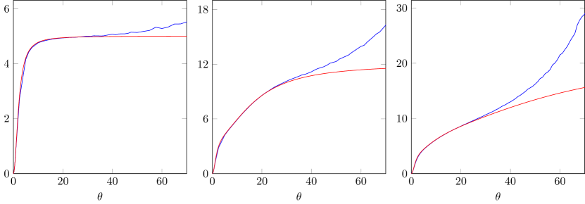
Figure 1: Square integral observational model Equation (13). Numerical Fisher information $I_{\theta_{0}}$ (blue) and the misspecified inverse variance $V_{\theta^{*}}$ (red) for dimensions $p=1,2$ and 3.

We considered the observational model with $p=1,2$ and $3$ coordinates and evaluated the true and misspecified Fisher informations for a wide collection of true shift parameters $\theta_{0}$, ranging from $\theta_{0}=0$ to $\theta_{0}=70$. The corresponding Fisher informations are plotted in Figure 1, using blue for the true and red for the misspecified information. For small values of $\theta_{0}$ they are aligned, and the misspecified model provides similar uncertainty quantification as the well-specified one. However, for large values of $\theta_{0}$ the scissor opens and there is a significant and increasing discrepancy between the two informations. We observe that the misspecified Fisher information gets substantially smaller than the true one, resulting in overly conservative credible sets in the misspecified model, for all choices of $p=1,2,3$.

We also compared the true and misspecified posterior distributions and their Gaussian approximations, where we varied the sample sizes over $N=50,250$, and $1250$ and took the shift parameter equal to $\theta_{0}=2$ or $\theta_{0}=40$, examples for which the true and misspecified Fisher informations match or not. In the former case, we considered a uniform prior for $\theta$ supported on the interval $[1,3]$. Figure 2 shows in blue and red the true and the misspecified posterior distributions in the case $\theta_{0}=2$, where dashed curves are their Gaussian approximations. One can see that both the true and misspecified posteriors concentrate around the true parameter $\theta_{0}$, their spread decreases at the same rate, and in both cases the Gaussian approximations are accurate. Figure 3 shows the same curves in the case $\theta_{0}=40$. By comparing the true density to the misspecified density, it can be seen that the centring points of the densities differ slightly. However, the interval where the centred 95% credible intervals intersect, remains large.

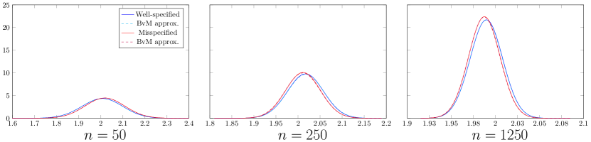
Figure 2: Square integral observational model Equation (13). True (blue) and misspecified (red) posterior densities and corresponding limiting Gaussian approximations in the case that the true shift parameter is $\theta_{0}=2$. The true curve is solid and the dashed curve is the Gaussian approximation. The sample size increases from left to right $N=50,250$, and $1250$.

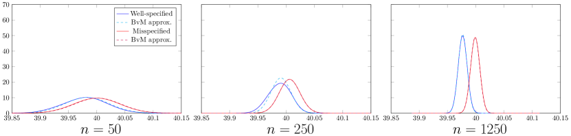
Figure 3: Square integral observational model Equation (13). True (blue) and misspecified (red) posterior densities and corresponding limiting Gaussian approximations in the case that the true shift parameter is $\theta_{0}=40$. The true curve is solid and the dashed curve is the Gaussian approximation. The sample size increases from left to right $N=50,250$, and $1250$.

5.2 Schrödinger equation

We consider the observational model Equation (16) resulting from the time-independent Schrödinger equation (15), investigated in Section 4.2. We choose $\mathcal{O}$ equal to the unit square, and in the first layer of the hierarchical model we take $f(x,y)=e^{2B_{1}(x)+3B_{2}(y)}$, for $(x,y)\in[0,1]^{2}$, where $B_{1},B_{2}$ are i.i.d. standard Brownian motions. Furthermore, we set the boundary condition to $g_{\theta}(x,y)=(x-\frac{1}{2})^{2}+\theta^{2}y$, for $(x,y)\in\partial[0,1]^{2}$.

We focus on comparing the true and misspecified Fisher informations $I_{\theta}$ and $V_{\theta^{*}}$, for values of the true parameter ranging from $\theta_{0}=0$ to $\theta_{0}=10$. We considered the $p=1$, 2 and 3-dimensional observational models. The true Fisher information was computed numerically from Equation (26). We simulated a Brownian motion $(\tilde{B}_{t})_{t\geq 0}$ and function $f$ on an equidistantly spaced $100\times 100$ grid of $[0,1]^{2}$. For each $X_{i}$, we drew $100$ i.i.d. observations of $f$, and used these to estimate the Fisher information through Equation (18). We used the basis functions $e_{i}(x)e_{j}(y)$ for $0\leq i,j\leq 3$, where $e_{i}$ denotes the $i$th normalized Legendre basis on $[0,1]$.

Figure 4 shows the true (blue) and misspecified (red) Fisher informations as a function of $\theta_{0}$. One observes that there is a slight deviation between the two informations. For $p=1$, the misspecified Fisher information dominates the true Fisher information, but for $p=3$ the true Fisher dominates the misspecified Fisher information.

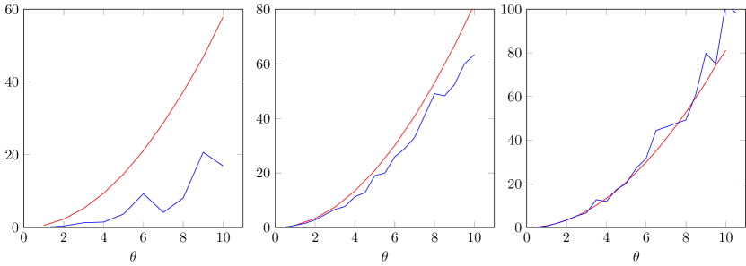
Figure 4: Schrödinger model (16). True Fisher information $I_{\theta_{0}}$ (blue) and misspecified Fisher information $V_{\theta_{0}}$ (red) as function of $\theta_{0}$ for observations of dimensions $p\times p$ with $p=1,3$ and $4$ (left to right).

6 Proof of the hierarchical Bernstein von-Mises theorem

In this section, we give the proofs of Lemma 1 and Theorem 1.

6.1 Proof of Lemma 1

For simplicity, we omit the index $i$ from the notation.

We show the more general statement that the Kullback-Leibler divergence is uniquely minimized at $(\mu,\Sigma)=(\mu_{\theta_{0}},\Sigma_{\theta_{0}})$, from which it follows that $\theta^{*}=\theta_{0}$ is the minimizer of $\theta\mapsto P_{0}\log(p_{0}/p_{\theta})$.

Up to an additive constant minus twice the log-likelihood of the normal distribution with mean $\mu$ and covariance matrix $\Sigma$ is equal to $\log\det\Sigma+(X-\mu)^{\intercal}\Sigma^{-1}(X-\mu)$. The expectation of this relative to an arbitrary distribution with $\mathbb{E}X=\mu_{\theta_{0}}$ and covariance matrix $\mathop{\mathrm{Cov}}\nolimits X=\Sigma_{\theta_{0}}$ is equal to

$$\log\det\Sigma+\mathbb{E}\bigl{(}(X-\mu_{\theta_{0}})^{\intercal}\Sigma^{-1}(X-\mu_{\theta_{0}})+(\mu-\mu_{\theta_{0}})^{\intercal}\Sigma^{-1}(\mu-\mu_{\theta_{0}})^{\intercal}$$

$$\qquad=\log\det\Sigma+\mathop{\text{tr}}\nolimits(\Sigma_{\theta_{0}}\Sigma^{-1})+(\mu-\mu_{\theta_{0}})^{\intercal}\Sigma^{-1}(\mu-\mu_{\theta_{0}}).$$

This is clearly minimized at $\mu=\mu_{\theta_{0}}$. It remains to find the minimizer of $\Sigma\mapsto\log\det(\Sigma)+\mathop{\text{tr}}\nolimits(\Sigma^{-1}\Sigma_{\theta_{0}})$. Taking $B:=\Sigma_{\theta_{0}}^{-1/2}\Sigma\Sigma_{\theta_{0}}^{-1/2}\succ 0$, equivalently we aim to minimize

$$B\mapsto\log\det(\Sigma_{\theta_{0}}^{1/2}B\Sigma_{\theta_{0}}^{1/2})+\mathrm{tr}(B^{-1}) =\log\det\Sigma_{\theta_{0}}+\log\det B+\mathrm{tr}(B^{-1}).$$

Let $(\lambda_{j})_{j=1,\ldots,p}$ denote the eigenvalues of $B$. Then the above expression simplifies to $c+\sum_{j=1}^{p}\log\lambda_{j}+\lambda_{j}^{-1}$, which is minimized at $\lambda_{j}=1$, for all $j=1,\ldots,p$. Hence the minimizer is $\Sigma=\Sigma_{\theta_{0}}$.

We now verify the formula for the Hessian at $\theta=\theta_{0}$. The second derivative of the Kullback-Leibler divergence with respect to $\theta_{l}$ and $\theta_{k}$ is given by

$$\frac{d^{2}}{d\theta_{l}d\theta_{k}}P_{0}\log(p^{o}/p_{\theta})|_{\theta=\theta_{0}}=-\frac{1}{2}\det(\Sigma_{\theta_{0}})^{-2}\Bigl{(}\frac{d}{d\theta_{l}}\det(\Sigma_{\theta_{0}})\Bigr{)}\biggl{(}\frac{d}{d\theta_{k}}\det(\Sigma_{\theta_{0}})\biggr{)}$$

$$\quad+\frac{1}{2}\det(\Sigma_{\theta_{0}})^{-1}\frac{d^{2}}{d\theta_{l}d\theta_{k}}\det(\Sigma_{\theta_{0}})+\biggl{(}\frac{d}{d\theta_{l}}\mu_{\theta_{0}}\biggr{)}^{\intercal}\Sigma_{\theta_{0}}^{-1}\biggl{(}\frac{d}{d\theta_{k}}\mu_{\theta_{0}}\biggr{)}$$

$$\quad+\frac{1}{2}\sum_{i,j}\Sigma_{\theta_{0},i,j}\frac{d^{2}}{d\theta_{l}d\theta_{k}}\Sigma_{\theta_{0},i,j}^{-1}.$$

Combining this with Lemmas 3 and 4, we see that

$$\frac{d^{2}}{d\theta_{l}d\theta_{k}}P_{0}\log(p_{0}/p_{\theta})|_{\theta=\theta_{0}}-\biggl{(}\frac{d}{d\theta_{l}}\mu_{\theta_{0}}\biggr{)}^{\intercal}\Sigma_{\theta_{0}}^{-1}\biggl{(}\frac{d}{d\theta_{k}}\mu_{\theta_{0}}\biggr{)}$$

$$\qquad=\frac{1}{2}\mathop{\text{tr}}\nolimits\biggl{(}\Sigma_{\theta_{0}}^{-1}\frac{d^{2}}{d\theta_{l}d\theta_{k}}\Sigma_{\theta_{0}}\biggr{)}-\frac{1}{2}\mathop{\text{tr}}\nolimits\biggl{(}\Sigma_{\theta_{0}}^{-1}\biggl{(}\frac{d}{d\theta_{l}}\Sigma_{\theta_{0}}\biggr{)}\Sigma_{\theta_{0}}^{-1}\biggl{(}\frac{d}{d\theta_{k}}\Sigma_{\theta_{0}}\biggr{)}\biggr{)}$$

$$\qquad+\frac{1}{2}\mathop{\text{tr}}\nolimits\biggl{(}\Sigma_{\theta_{0}}\frac{d^{2}}{d\theta_{l}d\theta_{k}}\Sigma_{\theta_{0}}^{-1}\biggr{)}.$$

By applying Equation (30) twice, we obtain

$$\frac{d^{2}}{d\theta_{l}d\theta_{k}}\Sigma_{\theta}^{-1} =\Sigma_{\theta}^{-1}\biggl{(}\frac{d}{d\theta_{l}}\Sigma_{\theta}\biggr{)}\Sigma_{\theta}^{-1}\biggl{(}\frac{d}{d\theta_{k}}\Sigma_{\theta}\biggr{)}\Sigma_{\theta}^{-1}-\Sigma_{\theta}^{-1}\biggl{(}\frac{d^{2}}{d\theta_{l}d\theta_{k}}\Sigma_{\theta}\biggr{)}\Sigma_{\theta}^{-1}$$

$$+\Sigma_{\theta}^{-1}\biggl{(}\frac{d}{d\theta_{k}}\Sigma_{\theta}\biggr{)}\Sigma_{\theta}^{-1}\biggl{(}\frac{d}{d\theta_{l}}\Sigma_{\theta}\biggr{)}\Sigma_{\theta}^{-1}.$$

Plugging this expression into the formula one before the previous display results in

$$\frac{d^{2}}{d\theta_{l}d\theta_{k}}P_{0}\log(p_{0}/p_{\theta})|_{\theta=\theta_{0}}$$ (19)

$$\qquad=\frac{1}{2}\mathop{\text{tr}}\nolimits\biggl{(}\Sigma_{\theta_{0}}^{-1}\biggl{(}\frac{d}{d\theta_{l}}\Sigma_{\theta_{0}}\biggr{)}\Sigma_{\theta_{0}}^{-1}\biggl{(}\frac{d}{d\theta_{k}}\Sigma_{\theta_{0}}\biggr{)}\biggr{)}+\biggl{(}\frac{d}{d\theta_{l}}\mu_{\theta_{0}}\biggr{)}^{\intercal}\Sigma_{\theta_{0}}^{-1}\biggl{(}\frac{d}{d\theta_{k}}\mu_{\theta_{0}}\biggr{)}.$$

This in turn implies the formula in Equation (8) for $V_{\theta^{*}}$.

Now note that Equation (8) can be rewritten in the form

$$\frac{1}{2}\sum_{1\leq k,l\leq p}(A_{1,kl},\ \ldots,\ A_{p,kl})(A_{1,kl},\ \ldots,\ A_{p,kl})^{\intercal}+[v_{1}^{\intercal},\ldots,v_{p}^{\intercal}][v_{1}^{\intercal},\ldots,v_{p}^{\intercal}]^{\intercal},$$

where $A_{l}=(A_{l,kl})_{k,l=1,\ldots,p}$. This expression is the sum of Gram matrices and hence is positive semi-definite. If the vectors $v_{j}$, $j=1,\ldots,d$ are linearly independent, then the second Gram matrix is positive definite, which implies the positive definiteness of $V_{\theta^{*}}$

6.2 Proof of Theorem 1

Below we verify Assumptions 1, with $\theta_{N}^{*}=\theta_{0}$ and $V_{\theta_{N}^{*},N}$ equal to the Hessian of the Kullback-Leibler divergence. Then the theorem is implied by Proposition 1 and Lemma 1.

Assumption assum:BvM theorem.1. The minimizing point $\theta_{N}^{*}=\theta_{0}$ is independent of $N$ and is interior to $\Theta$ by assumption.

Assumption assum:BvM theorem.2. In the case that the mean and covariance functions do not depend on $i$, the Hessian is given by Equation (8). In the case that they do depend on $i$, the average Hessians converge by assumption. In both cases, the (limiting) Hessian $V_{\theta_{0}}$ is positive definite by assumption.

Assumption assum:BvM theorem.3. Because the Kullback-Leibler divergence is minimized at $\theta=\theta_{0}$, its gradient vanishes at this point. This implies that $\nabla l^{(N)}(\theta_{0})$ has mean zero. The random vector $\nabla l^{(N)}(\theta_{0})$ is a sum of independent variables, each a polynomial of degree $2$ in the observations $X_{i,k}$, $k=1,\ldots,p$ . Therefore $\mathop{\mathrm{Var}}\nolimits_{P_{0}}\bigl{(}N^{-1/2}\nabla l^{(N)}(\theta_{0})\bigr{)}\lesssim N^{-1}\sum_{i=1}^{N}P_{0,i}\|X_{i}\|_{2}^{4}$. Because $\sup_{i}P_{0,i}\|X_{i}\|_{2}^{4}<\infty$ by assumption, the variances are bounded in $N$. Combined with the vanishing means, this implies that the sequence $N^{-1/2}\nabla l^{(N)}(\theta_{0})$ is bounded in probability.

Assumption assum:BvM theorem.4. By the formula for the expected log Gaussian likelihood given in the proof of Lemma 1, we have that $2N^{-1}P_{0}\bigl{(}l^{(N)}(\theta)-l^{(N)}(\theta_{0})\bigr{)}$ is equal to minus the average given in Equation (1). In the case that the mean and variance functions $\mu_{\theta}^{(i)}$ and $\Sigma_{\theta}^{(i)}$ do not depend on $i$, these averages are fixed in $N$. In view of Lemma 1 and the assumptions, these averages are positive for every $\theta\not=\theta_{0}$. Furthermore, as a function of $\theta$ they are continuous. Since $\Theta$ is compact, it follows that the averages are bounded away from zero on the set $\{\theta:\|\theta-\theta_{0}\|\geq\delta\}$, for every $\delta>0$. In the case that the mean and covariance functions do depend on $i$, this is true by assumption. Therefore, for the verification of Assumption assum:BvM theorem.4, it suffices to show that $\sup_{\theta}N^{-1}\bigl{|}\bigl{(}l^{(N)}(\theta)-l^{(N)}(\theta_{0})\bigr{)}-P_{0}\bigl{(}l^{(N)}(\theta)-l^{(N)}(\theta_{0})\bigr{)}\bigr{|}$ tends to zero in probability.

We prove this using a bracketing argument, as given in Lemma 2. The Gaussian log-likelihood can be written in exponential family form as

$$l^{(N)}(\theta)=c_{N}(\theta)-\sum_{i=1}^{N}\sum_{k=1}^{K}T_{i,k}(X_{i})g_{i,k}(\theta)$$ (20)

with sufficient statistics and natural parameter vectors given by

$$T_{i}(X_{i})=\begin{pmatrix}X_{i}\\ \mathop{\text{vec}}\nolimits\big{(}X_{i}X_{i}^{\intercal}\big{)}\end{pmatrix}\qquad\text{and}\qquad g_{i}(\theta)=\begin{pmatrix}(\Sigma_{\theta}^{(i)})^{-1}\mu_{\theta}^{(i)}\\ -\frac{1}{2}\mathop{\text{vec}}\nolimits\big{(}(\Sigma_{\theta}^{(i)})^{-1}\big{)}\end{pmatrix}.$$ (21)

Here $\mathop{\text{vec}}\nolimits(A)$ denotes a column vector constructed from the elements of a matrix $A$ (in an arbitrary, but fixed way). By assumption the functions $\theta\mapsto(\Sigma_{\theta}^{(i)})^{-1}$ and $\theta\mapsto\mu_{\theta}^{(i)}$ are twice differentiable with equicontinuous second derivatives. The same holds for the functions $\theta\mapsto g_{i,k}(\theta)$, $i=1,\ldots,N$ and $k=1,\ldots,K$.

It suffices to prove that $\sup_{\theta}\tfrac{1}{N}\bigl{|}\sum_{i=1}^{N}\bigl{(}T_{i,k}(X_{i})-P_{0}T_{i,k})\bigr{)}\bigl{(}g_{i,k}(\theta)-g_{i,k}(\theta_{0})\bigr{)}\bigr{|}$ tends to zero in probability, for every fixed $k$. For a given covering $\Theta=\cup_{j}B_{j}$ by balls of radius $\delta$, consider the brackets

$$\mathcalligra{l}_{i,j} =T_{i,k}^{+}\,\inf_{\theta\in B_{j}}\bigl{(}g_{i,k}(\theta)-g_{i,k}(\theta_{0})\bigr{)}-T_{i,k}^{-}\,\sup_{\theta\in B_{j}}\bigl{(}g_{i,k}(\theta)-g_{i,k}(\theta_{0})\bigr{)}$$

$$\mathcalligra{u}_{i,j} =T_{i,k}^{+}\,\sup_{\theta\in B_{j}}\bigl{(}g_{i,k}(\theta)-g_{i,k}(\theta_{0})\bigr{)}-T_{i,k}^{-}\,\inf_{\theta\in B_{j}}\bigl{(}g_{i,k}(\theta)-g_{i,k}(\theta_{0})\bigr{)}.$$

We have $\mathcalligra{l}_{i,j}\leq T_{i,k}\bigl{(}g_{i,k}(\theta)-g_{i,k}(\theta_{0})\bigr{)}\leq\mathcalligra{u}_{i,j}$, for all $\theta\in B_{j}$ and $i\in\mathbb{N}$, and

$$|\mathcalligra{u}_{i,j}-\mathcalligra{l}_{i,j}|\leq|T_{i,k}|\,\Bigl{|}\sup_{\theta\in B_{j}}g_{i,k}(\theta)-\inf_{\theta\in B_{j}}g_{i,k}(\theta)\Bigr{|}.$$

Because the functions $g_{i,k}$ are uniformly equicontinuous, for every given $\epsilon>0$ there exists $\delta>0$ such that the variation of $g_{i,k}$ over an arbitrary ball of radius $\delta$ is at most $\epsilon$. Because $\Theta$ is compact, for given $\delta>0$, there is a finite cover $\Theta=\cup_{j}B_{j}$ by balls of radius $\delta$. For such a cover the right side of the display is bounded above by $|T_{i,k}|\epsilon$, for every $j$ and $i$. It follows that $N^{-1}\sum_{i=1}^{N}P_{0}|\mathcalligra{u}_{i,j}-\mathcalligra{l}_{i,j}|\leq N^{-1}\sum_{i=1}^{N}P_{0}|T_{i,k}|\epsilon\lesssim\sup_{i}P_{0}\|X_{i}\|^{4}\epsilon$. Furthermore, since $\mathop{\mathrm{Var}}\nolimits T^{-}\vee\mathop{\mathrm{Var}}\nolimits T^{+}\leq\mathop{\mathrm{Var}}\nolimits T$ and $\mathop{\mathrm{Var}}\nolimits(S+T)\leq 2\mathop{\mathrm{Var}}\nolimits S+2\mathop{\mathrm{Var}}\nolimits T$, for any random variables $S,T$, we have

$$\frac{1}{N^{2}}\sum_{i=1}^{N}\bigl{(}\mathop{\mathrm{Var}}\nolimits_{P_{0}}\mathcalligra{l}_{i,j}(X_{i})+\mathop{\mathrm{Var}}\nolimits_{P_{0}}\mathcalligra{u}_{i,j}(X_{i})\bigr{)}$$

$$\qquad\leq\frac{4}{N^{2}}\sum_{i=1}^{N}\mathop{\mathrm{Var}}\nolimits_{P_{0}}T_{i,k}(X_{i})\max_{j}\sup_{\theta\in B_{j}}\bigl{|}g_{i,k}(\theta)-g_{i,k}(\theta_{0})\bigr{|}^{2},$$

which tends to zero as $N\to\infty$.

Assumption assum:BvM theorem.5. By using the Taylor expansion of $l^{(N)}(\theta)$ around $\theta^{*}$, we obtain that

$$l^{(N)}(\theta)-l^{(N)}(\theta^{*})$$

$$\qquad=\nabla l^{(N)}(\theta^{*})^{\intercal}(\theta-\theta^{*})+\frac{1}{2}(\theta-\theta^{*})^{\intercal}\sum_{i=1}^{N}\sum_{k=1}^{K}H^{g_{i,k}}_{\theta^{*}}(\theta)T_{i,k}(X_{i})(\theta-\theta^{*}),$$

where $H^{g_{i,k}}_{\theta^{*}}(\theta)$, are symmetric matrices with value at index $(r,s)$ given by

$$H^{g_{i,k}}_{\theta^{*},r,s}(\theta)=2\int_{0}^{1}(1-t)\frac{\partial^{2}}{\partial\theta_{r}\partial\theta_{s}}g_{i,k}(\theta^{*}+t(\theta-\theta^{*}))\,dt.$$ (22)

Since $V_{\theta^{*},N}$ is defined as the Hessian of $N^{-1}l^{(N)}(\theta)$ at $\theta^{*}$, we have

$$-V_{\theta^{*},N}=\frac{1}{N}\sum_{i=1}^{N}\sum_{k=1}^{K}H_{\theta^{*}}^{g_{i,k}}(\theta^{*})P_{0,i}(T_{i,k}(X_{i})),$$

and arrive at

$$\frac{1}{N}R_{N}(\theta)=\frac{1}{N}\sum_{i=1}^{N}\biggl{(}\sum_{k=1}^{K}(H^{g_{i,k}}_{\theta^{*}}(\theta^{*})P_{0,i}T_{i,k}(X_{i})-H^{g_{i,k}}_{\theta^{*}}(\theta)T_{i,k}(X_{i}))\biggr{)}.$$ (23)

By the triangle inequality this is bounded above by

$$\frac{1}{N}\Bigl{\|}\sum_{i=1}^{N}\sum_{k=1}^{K}H^{g_{i,k}}_{\theta^{*}}(\theta^{*})\Bigl{(}T_{i,k}(X_{i})-P_{0,i}T_{i,k}(X_{i})\Bigr{)}\Bigr{\|}$$

$$+\max_{i,k}\sup_{\theta:\|\theta-\theta^{*}\|\leq\delta}\big{(}H^{g_{i,k}}_{\theta^{*}}(\theta^{*})-H^{g_{i,k}}_{\theta^{*}}(\theta)\big{)}\frac{1}{N}\sum_{i=1}^{N}\sum_{k=1}^{K}P_{0,i}|T_{i,k}(X_{i})|.$$

The first term is an average of independent random variables with mean zero and bounded variances, and hence this term tends to zero in probability. The second term can be made arbitrarily small by choice of $\delta$, by the equicontinuity of the functions $H^{g_{i,k}}_{\theta^{*}}$.

Assumption assum:BvM theorem.6. This is true by assumption.

Lemma 2.

For $i\in\mathbb{N}$ and $\theta\in\Theta$, let $f_{i,\theta}:\mathbb{R}^{d}\to\mathbb{R}$ be a measurable function. Assume that for every $\epsilon>0$, there exist functions $\mathcalligra{l}_{i,j},\mathcalligra{u}_{i,j}:\mathbb{R}^{d}\to\mathbb{R}$, for $j=1,\ldots,J_{\epsilon}$ and $i\in\mathbb{N}$ such that for every $\theta\in\Theta$ there exists a $j\in\{1,\ldots,J_{\epsilon}\}$ such that $\mathcalligra{l}_{i,j}\leq f_{i,\theta}\leq\mathcalligra{u}_{i,j}$ for every $i\in\mathbb{N}$, and such that

$$\limsup_{N\to\infty}\frac{1}{N}\sum_{i=1}^{N}\mathbb{E}\big{(}\mathcalligra{u}_{i,j}(X_{i})-\mathcalligra{l}_{i,j}(X_{i})\big{)} \leq\epsilon$$

$$\lim_{N\to\infty}N^{-2}\sum_{i=1}^{N}\frac{1}{N}\sum_{i=1}^{N}\bigl{(}\mathop{\mathrm{Var}}\nolimits\mathcalligra{l}_{i,j}(X_{i})+\mathop{\mathrm{Var}}\nolimits\mathcalligra{u}_{i,j}(X_{i})\bigr{)} =0,$$

for every $j\in\{1,\ldots,J_{\epsilon}\}$. Then $\frac{1}{N}\sup_{\theta\in\Theta}\bigl{|}\sum_{i=1}^{N}\bigl{(}f_{i,\theta}(X_{i})-\mathbb{E}f_{i,\theta}(X_{i})\bigr{)}\bigr{|}\to 0$ in probability.

Proof.

Take arbitrary $\theta\in\Theta$. By assumption there exists a $j\in\{1,\ldots,J_{\epsilon}\}$ such that, for $N$ large enough,

$$\frac{1}{N}\sum_{i=1}^{N}\bigl{[}f_{i,\theta}(X_{i})-P_{i}f_{i,\theta}\bigr{]} \leq\frac{1}{N}\sum_{i=1}^{N}\bigl{(}\mathcalligra{u}_{i,j}(X_{i})-P_{i}\mathcalligra{u}_{i,j}\bigr{)}+\frac{1}{N}\sum_{i=1}^{N}P_{i}(\mathcalligra{u}_{i,j}-\mathcalligra{l}_{i,j})$$

$$\leq\frac{1}{N}\sum_{i=1}^{N}\bigl{(}\mathcalligra{u}_{i,j}(X_{i})-P_{i}\mathcalligra{u}_{i,j}\bigr{)}+\epsilon.$$

Hence the supremum over $\theta$ of the left side is bounded above by

$$\max_{j=1,\ldots,J_{\epsilon}}\frac{1}{N}\sum_{i=1}^{N}\bigl{(}\mathcalligra{u}_{i,j}(X_{i})-P_{i}\mathcalligra{u}_{i,j}\bigr{)}+\epsilon.$$

By the assumption $\lim_{N\to\infty}N^{-2}\sum_{i=1}^{N}\mathop{\mathrm{Var}}\nolimits\mathcalligra{u}_{i,j}(X_{i})=0$, this tends in probability to $\epsilon$. In combination with a similar argument using the lower brackets $\mathcalligra{l}_{i,j}$, we find that the sequence given by $N^{-1}\sup_{\theta\in\Theta}\bigl{|}\sum_{i=1}^{N}\bigl{(}f_{i,\theta}(X_{i})-\mathbb{E}f_{i,\theta}(X_{i})\bigr{)}\bigr{|}\to 0$ is asymptotically bounded in probability by $\epsilon$. This being true for every $\epsilon>0$, gives the result. ∎

7 Proofs for the applications

In this section, we collect the proofs for the three examples discussed in Section 4. In each case we verify that the conditions of Theorem 1 hold.

7.1 Proof of Corollary 1

The mean function $\theta\mapsto\mu_{\theta}^{(i)}$ is given in Equation (12) with $z=z_{i}$. These functions are twice differentiable, and for bounded set $\{z_{i}:\,i\in\mathbb{N}\}$ the second derivative is bounded and equicontinuous.

Next, we deal with the function $\theta\mapsto\Sigma_{\theta}^{(i)}$. For $k,l\in\mathbb{N}_{0}$, define the coefficients

$$b_{k,l} =\frac{2}{3}((4+k)^{-1}(k+l+6)^{-1}+(k+2)^{-1}((l+4)^{-1}-(k+l+6)^{-1}))$$

$$-\frac{1}{3}((5+k)^{-1}(k+l+6)^{-1}+(k+1)^{-1}((l+5)^{-1}-(k+l+6)^{-1}))$$

and

$$c_{k,l} =2((k+3)^{-1}(k+l+5)^{-1}+(k+2)^{-1}((l+3)^{-1}-(k+l+5)^{-1}))$$

$$-\frac{2}{3}((k+4)^{-1}(k+l+5)^{-1}+(k+1)^{-1}((l+4)^{-1}-(k+l+5)^{-1}))).$$

Then for all $j_{1},j_{2}\in\mathbb{N}_{0}$, we have

$$\Sigma_{\theta,j_{1},j_{2}}^{(i)}=\Lambda_{j_{1},j_{2}}+\sum_{k=0}^{j_{1}}\sum_{l=0}^{j_{2}}a_{j_{1},l}a_{j_{2},k}(z_{i}^{5}b_{k,l}+\theta^{2}z_{i}^{4}c_{k,l}).$$ (24)

See Section 8.0.1 for the details of the cumbersome, but elementary computations to derive this result. The limiting covariance matrix of the misspecified posterior, given in Equation (8), is completely determined by Equations (12) and (24).

The function $\theta\mapsto\Sigma_{\theta,j_{1},j_{2}}^{(i)}$ is twice differentiable and for bounded set $\{z_{i}:\,i\in\mathbb{N}\}$ the second derivative is bounded and equicontinuous. Also note that the matrix can be written in the form $\Sigma_{\theta}^{(i)}=\Lambda+Az_{i}^{5}+\theta^{2}z_{i}^{4}B$ for positive semi-definite matrices $\Lambda,B$ and $C$ not depending on $z_{i}\geq 0$ or $\theta\in\mathbb{R}$ (the positive semi-definiteness of $B$ and $C$ follows from the positive semi-definiteness of $\Sigma_{\theta}$ for all $z_{i}>0$ and $\theta\in\mathbb{R}$). Using the above formula one can compute the misspecified posterior covariance matrix given in Equation (8). In view of $\frac{d}{d\theta}\mu_{\theta}=\theta z^{3/2}(1,\tfrac{1}{3},0,\ldots,0)$, we get that

$$V_{\theta^{*}}^{(i)} =\frac{1}{2}\mathop{\text{tr}}\nolimits\biggl{(}\Bigl{[}\bigl{(}\Lambda+Az_{i}^{5}+B\theta_{0}^{2}z_{i}^{4}\bigr{)}^{-1}2\theta_{0}Bz_{i}^{4}\Bigr{]}^{2}\biggr{)}$$

$$\quad+\theta_{0}z_{i}^{3/2}(1,\tfrac{1}{3},0,\ldots,0)\bigl{(}\Lambda+Az_{i}^{5}+B\theta_{0}^{2}z_{i}^{4}\bigr{)}^{-1}\theta_{0}z_{i}^{3/2}(1,\tfrac{1}{3},0,\ldots,0)^{\intercal}$$

$$=z_{i}^{8}G_{\theta_{0},1}(z_{i})+z_{i}^{3}G_{\theta_{0},2}(z_{i})$$

with functions $G_{\theta_{0},1}(z)$ and $G_{\theta_{0},2}(z)$ such that $\sup_{0\leq z\leq C}|G_{\theta_{0},1}(z)|+|G_{\theta_{0},2}(z)|<\infty$ for arbitrary $C>0$. One can immediately obtain that $V_{\theta^{*}}^{(i)}>0$ if and only if $\theta^{*}=\theta_{0}\neq 0$.

Since $\Theta$ and $(z_{i})_{i\in\mathbb{N}}$ are bounded, we know that $\mu_{\theta,j}^{(i)}$ are uniformly bounded. Furthermore, in view of

$$\Sigma_{\theta}^{-1}\leq\Lambda^{-1},$$

the elements of $\Sigma_{\theta}^{-1}$ are bounded in absolute value.

The map $(\theta,z)\mapsto\mu_{\theta,z}$ is continuous. Since $\Theta\times\overline{\{z_{i}:i\in\mathbb{N}\}}$ is compact, it is uniformly continuous. Similarly, $(\theta,z)\mapsto\Sigma_{\theta,z}$ is uniformly continuous. Note also that the function $\theta\mapsto\Sigma_{\theta,z}$ is twice differentiable and the second derivative is also equicontinuous. Furthermore, since $\det(\Sigma_{\theta,z})\geq\det(\mathop{\mathrm{Cov}}\nolimits(\eta_{z,\theta}(f_{i})))+\det(\Lambda)\geq\det(\Lambda)$ is lower bounded for all $(\theta,z)\in\Theta\times\{z_{i}:i\in\mathbb{N}\}$, the function $(\theta,z)\mapsto\Sigma_{\theta,z}^{-1}$ is uniformly continuous as well. For the case where the sequence $(z_{i})_{i\in\mathbb{N}}$ is constant we have i.i.d. data and therefore $\lim_{N\to\infty}V_{\theta^{*},N}=V_{\theta^{*}}>0$. If $z_{i}\rightarrow 0$, then $\lim_{z_{i}\to 0}V_{\theta*}^{(i)}=0$, and thus $\lim_{N\to\infty}N^{-1}\sum_{i=1}^{N}V_{\theta^{*}}^{(i)}=0$.

In order to show that Equation (1) holds, we first note that the Kullback-Leibler divergence between a $N(0,\Sigma_{\theta})$ distribution, and a $N(0,\Sigma_{\theta_{0}})$ distribution is equal to the difference $\mathop{\text{tr}}\nolimits\bigl{(}\Sigma_{\theta_{0}}^{(i)}\bigl{(}\Sigma_{\theta}^{(i)}\bigr{)}^{-1}-I\bigr{)}-\log\det\bigl{(}\Sigma_{\theta_{0}}^{(i)}\bigl{(}\Sigma_{\theta}^{(i)}\bigr{)}^{-1}\bigr{)}$. Hence this term must be non-negative. Therefore it suffices to show that

$$\limsup_{N\to\infty}\sup_{\theta:|\theta-\theta_{0}|\geq\delta}\frac{1}{N}\sum_{i=1}^{N}(\mu_{\theta}^{(i)}-\mu_{\theta_{0}}^{(i)})^{\intercal}(\Sigma_{\theta}^{(i)})^{-1}(\mu_{\theta}^{(i)}-\mu_{\theta_{0}}^{(i)})>0.$$

With $\lambda_{1}^{(i)},\ldots,\lambda_{d}^{(i)}$ the eigenvalues of $\Sigma_{\theta}^{(i)}$, the left-hand side of the previous display is lower-bounded by

$$\limsup_{N\to\infty}\sup_{\theta:|\theta-\theta_{0}|\geq\delta}\frac{1}{N}\sum_{i=1}^{N}\inf_{j=1,\ldots,d}(\lambda_{j}^{(i)})^{-1}\|\mu_{\theta}^{(i)}-\mu_{\theta_{0}}^{(i)}\|^{2}.$$ (25)

We first lower bound $\inf_{j=1,\ldots,d}(\lambda_{j}^{(i)})^{-1}$ uniformly in $i$, which is equivalent to giving an upper bound for the eigenvalues of $\Sigma_{\theta}^{(i)}=\mathop{\mathrm{Cov}}\nolimits(T_{z_{i},\theta}(f))+\Lambda$ that is uniform in $i$. The uniform boundedness of the coefficients $a_{k,l}$, $b_{k,l}$ and $c_{k,l}$ combined with Equation (24) shows that the elements of $\Sigma_{\theta_{0}}^{(i)}$ are uniformly bounded as long as $(z_{i})_{i\in\mathbb{N}}$ is bounded. This in turn shows that the eigenvalues of $\Sigma_{\theta_{0}}^{(i)}$ are uniformly upper bounded, if the sequence $(z_{i})_{i\in\mathbb{N}}$ is bounded. Therefore we see that $\inf_{j=1,\ldots,d}(\lambda_{j}^{(i)})^{-1}$ is lower bounded by some fixed constant. This shows that the eigenvalues of $\Sigma_{\theta_{0}}^{(i)}$ are uniformly bounded as well. In order to lower bound $\|\mu_{\theta}^{(i)}-\mu_{\theta_{0}}^{(i)}\|^{2}$, we Equation (12) to see that

$$\|\mu_{\theta}^{(i)}-\mu_{\theta_{0}}^{(i)}\|^{2}=\frac{1}{3}z_{i}^{3}(\theta+\theta_{0})^{2}(\theta-\theta_{0})^{2}.$$

This is lower bounded by $\frac{1}{3}z_{i}^{3}|\theta+\theta_{0}|^{2}\delta^{2}$ for all $\theta\in\Theta$ such that $|\theta-\theta_{0}|\geq\delta$. Therefore Equation (25) is lower bounded, up to some fixed constant, by

$$\limsup_{N\to\infty}\frac{1}{N}\sum_{i=1}^{N}z_{i}^{3},$$

which is positive by assumption.

We finish the proof by providing upper bounds for the fourth moment. By Jensen’s inequality and Fubini’s theorem, we have

$$P_{0}^{(N)}|\langle T_{\theta,i}f,e_{i,j}\rangle|^{4} \leq\int_{0}^{z_{i}}\int_{0}^{t}P_{0}^{(N)}(f(s)-\theta)^{8}ds|e_{i,j}(t)|^{4}\,dt<\infty,$$

where in the last inequality we used that $f(s)\sim\mathcal{N}(0,s)$, implying a finite eighth moment.

7.2 Proof of Corollary  2

In view of the maximum principle (see Theorem $4$ in Chapter 6.4 of Evans (2010)), for all $x\in\mathcal{O}$,

$$0\wedge\inf_{y\in\partial\mathcal{O}}g_{\theta_{0}}(y)\leq T_{\theta_{0}}f(x)\leq 0\vee\sup_{y\in\partial\mathcal{O}}g_{\theta_{0}}(y),$$

implying $P_{0}^{(N)}\|X_{i}\|^{4}<\infty$.

Proposition $25$ in Nickl (2018) implies that the solution $T_{\theta}f$ can be represented by the Feynman-Kac formula

$$T_{\theta}f(x)=\mathbb{E}^{x}\biggl{(}g_{\theta}(\tilde{B}_{\tau_{\mathcal{O}}})e^{-\int_{0}^{\tau_{\mathcal{O}}}f(\tilde{B}_{s})ds}\biggr{)}.$$ (26)

Here $(\tilde{B}_{s}:s\geq 0)$ denotes a $d$-dimensional Brownian motion, where the superscript $x$ denotes the fact that it has started at $x\in\mathcal{O}$. Here $\tau_{\mathcal{O}}$ is the exit time of $(\tilde{B}_{s})_{s\geq 0}$ from $\mathcal{O}$. Recall that the multivariate Gaussian model belongs to the exponential family of distributions Equation (20), with natural parameter vector $g_{\theta}$ and sufficient statistics vector $T_{i}(X_{i})$ given in Equation (21). In view of the regularity assumptions on $\theta\mapsto\mu_{\theta}$ and $\theta\mapsto\Sigma_{\theta}$, one can apply Fubini’s theorem twice in the Feynman-Kac formula, and conclude

$$\frac{d}{d\theta_{j}}P_{0}^{(N)}\langle T_{\theta}f,e_{l}\rangle =\int_{\mathcal{O}}\mathbb{E}^{x}\biggl{(}\frac{d}{d\theta_{j}}g_{\theta}(\tilde{B}_{\tau_{\mathcal{O}}})\mathbb{E}_{f}e^{-\int_{0}^{\tau_{\mathcal{O}}}f(\tilde{B}_{s})ds}\biggr{)}e_{l}(x)\,dx,$$ (27)

where $\mathbb{E}^{x}$ denotes the expectation with respect to Brownian motion starting at $x\in\mathcal{O}$, and $\mathbb{E}_{f}$ denotes the expectation with respect to the random variable $f$. Therefore, the map $\theta\mapsto\mu_{\theta}$ is smooth. We can extend this argument to show that these maps are differentiable to the same order as $\theta\mapsto g_{\theta}$ is differentiable and bounded. It follows that the map $\theta\mapsto P_{0}^{(N)}\log p_{\theta}$ is a composition of twice differentiable maps, and therefore twice differentiable. Reasoning along similar lines shows that $\theta\mapsto\mathop{\mathrm{Cov}}\nolimits_{\theta}(X_{i},X_{j})$ is twice differentiable.

Finally, to prove the positive definiteness of $V_{\theta^{*}}$, note that the linear independence assumption of the vectors $\frac{d}{d\theta_{j}}\mu_{\theta}\in\mathbb{R}^{p}$, for $j=1,\ldots,d$, implies that the vectors $v_{j}$, for $j=1,\ldots,d$, are linearly independent in Equation (8). Therefore, the second Gram matrix in Equation (8) is positive definite, which implies the positive definiteness of $V_{\theta^{*}}$.

7.3 Proof of Corollary 3

Define $X=(X_{t})_{t\in[0,t_{\max}]}$ to be the solution to the stochastic differential equation defined in terms of $a,b$ and $c_{\theta}$ and initial conditions $X_{0}=x\in\mathcal{O}$ (see Feehan, Gong and Song (2015)). By the Feynman-Kac formula the solution $u_{\theta}:(0,t_{\max})\times\mathcal{O}$ of Equation (17) can be expressed as

$$u_{\theta}(t,x) =\mathbb{E}^{x}\Biggl{(}g_{\theta}(\tau_{\mathcal{O}}\wedge t_{\max},X_{\tau_{\mathcal{O}}\wedge t_{\max}})\exp\biggl{(}-\int_{t}^{\tau_{\mathcal{O}}\wedge t_{\max}}c_{\theta}(X_{s})\,ds\biggr{)}\Biggr{)}$$ (28)

$$+\mathbb{E}^{x}\Biggl{(}\int_{t}^{\tau_{\mathcal{O}}\wedge t_{\max}}f(X_{s})\exp\biggl{(}-\int_{t}^{s}c_{\theta}(X_{v})\,dv\biggr{)}\,ds\Biggr{)}.$$

Here $\tau_{\mathcal{O}}=\tau_{\mathcal{O},x}$ is defined as the exit time of $X$ out of $\mathcal{O}$, i.e.

$$\tau_{\mathcal{O},x}=\inf\{s\geq 0:X_{s}\notin\mathcal{O}\},\qquad X_{0}=x.$$

Using this formula, we proceed by showing that the collections of functions $\{\theta\mapsto\mu_{\theta}^{(i)}:i\in\mathbb{N}\}$ and $\{\theta\mapsto\Sigma_{\theta}^{(i)}:i\in\mathbb{N}\}$ are equicontinuous. Let $\theta_{1},\theta_{2}\in\Theta$ be given. Note that

$$|\mu_{\theta_{1},l}^{(i)}-\mu_{\theta_{2},l}^{(i)}| \leq\|e_{l}\|_{\infty}\mathbb{E}_{g}\|u_{\theta_{1}}(t_{i},\cdot)-u_{\theta_{2}}(t_{i},\cdot)\|_{\infty}.$$

The second factor on the right-hand side of the preceding display can be bounded from above by triangle inequality as

$$\|u_{\theta_{1}}(t_{i},\cdot)-u_{\theta_{2}}(t_{i},\cdot)\|_{\infty}$$

$$\leq\mathbb{E}^{x}|g_{\theta_{1}}(\tau_{\mathcal{O}}\wedge t_{\max},X_{\tau_{\mathcal{O}}\wedge t_{\max}})|$$

$$\quad\times\underbrace{\Big{|}\exp\Big{(}-\int_{t}^{\tau_{\mathcal{O}}\wedge t_{\max}}c_{\theta_{1}}(X_{s})ds\Big{)}-\exp\Big{(}-\int_{t}^{\tau_{\mathcal{O}}\wedge t_{\max}}c_{\theta_{2}}(X_{s})ds\Big{)}\Big{|}}_{=:\Delta_{1}}$$

$$+\mathbb{E}^{x}\Big{|}\exp\Big{(}-\int_{t}^{\tau_{\mathcal{O}}\wedge t_{\max}}c_{\theta_{2}}(X_{s})ds\Big{)}\Big{|}$$

$$\quad\times\underbrace{|g_{\theta_{2}}(\tau_{\mathcal{O}}\wedge t_{\max},X_{\tau_{\mathcal{O}}\wedge t_{\max}})-g_{\theta_{1}}(\tau_{\mathcal{O}}\wedge t_{\max},X_{\tau_{\mathcal{O}}\wedge t_{\max}})|}_{=:\Delta_{2}}$$

$$+\mathbb{E}^{x}\!\int\limits_{t}^{\tau_{\mathcal{O}}\wedge t_{\max}}|f(X_{s})|\underbrace{\Big{|}\exp\Big{(}-\int_{t}^{s}c_{\theta_{1}}(X_{v})dv\Big{)}-\exp\Big{(}-\int_{t}^{s}c_{\theta_{2}}(X_{v})dv\Big{)}\Big{|}}_{=:\Delta_{3}}\ ds.$$

In view of the bounds

$$\Delta_{1} \leq t_{\max}\sup_{\theta\in\Theta}\|\nabla_{\theta}c_{\theta}\|_{\infty}\|\theta_{1}-\theta_{2}\|,$$

$$\Delta_{2} \leq\sup_{\theta\in\Theta}\|\nabla_{\theta}g_{\theta}\|_{\infty}\|\theta_{1}-\theta_{2}\|,$$

$$\Delta_{3} \leq t_{\max}\sup_{\theta\in\Theta}\|\nabla_{\theta}c_{\theta}\|_{\infty}\|\theta_{1}-\theta_{2}\|,$$

combined with the assumed bounds on $g_{\theta}$ and $c_{\theta}$, we find that

$$\|u_{\theta_{1}}(t_{i},\cdot)-u_{\theta_{2}}(t_{i},\cdot)\|_{\infty}\leq t_{\max}\sup_{\theta\in\Theta}\|g_{\theta}\|_{\infty}\sup_{\theta\in\Theta}\|\nabla_{\theta}c_{\theta}\|_{\infty}\|\theta_{1}-\theta_{2}\|$$

$$\qquad\qquad+\sup_{\theta\in\Theta}\|\nabla_{\theta}g_{\theta}\|_{\infty}\|\theta_{1}-\theta_{2}\|+t_{\max}^{2}\sup_{\theta\in\Theta}\|f\|_{\infty}\sup_{\theta\in\Theta}\|\nabla_{\theta}c_{\theta}\|_{\infty}\|\theta_{1}-\theta_{2}\|.$$ (29)

We conclude that $\{\theta\mapsto\mu_{\theta,l}^{(i)}:i\in\mathbb{N}\}$ is equicontinuous. Since the covariance term $\Sigma_{\theta,l,k}^{(i)}=P_{0,i}X_{\theta,i,l}X_{\theta,i,k}-P_{0,i}X_{\theta,i,l}P_{0,i}X_{\theta,i,k}$, and the second term is equicontinuous, we only need to show that $\theta\mapsto P_{0,i}X_{\theta,i,k}X_{\theta,i,l}$ is equicontinuous. We have

$$|P_{0,i}X_{\theta_{1},i,k}X_{\theta_{1},i,l}-P_{0,i}X_{\theta_{2},i,k}X_{\theta_{2},i,l}|$$

$$\qquad\qquad\leq\|e_{l}\|_{\infty}\|e_{k}\|_{\infty}P_{0,i}\int_{\mathcal{O}}\int_{\mathcal{O}}\Big{(}|u_{\theta_{1}}(t_{i},x)-u_{\theta_{2}}(t_{i},x)||u_{\theta_{1}}(t_{i},y)|$$

$$\qquad\qquad\qquad\qquad\qquad+|u_{\theta_{1}}(t_{i},y)-u_{\theta_{2}}(t_{i},y)||u_{\theta_{2}}(t_{i},x)|\Big{)}\,dx\,dy.$$

If we show that the first term of the integrand on the right-hand side is equicontinuous, the claim follows. By Hölder’s inequality, we bound the integral by

$$\mathbb{E}_{G}\int_{\mathcal{O}}\int_{\mathcal{O}}|u_{\theta_{1}}(t_{i},x)-u_{\theta_{2}}(t_{i},x)||u_{\theta_{1}}(t_{i},y)|\,dx\,dy$$

$$\qquad\qquad\qquad\leq\sqrt{\mathbb{E}_{G}\int_{\mathcal{O}}|u_{\theta_{1}}(t_{i},x)-u_{\theta_{2}}(t_{i},x)|\,dx^{2}\mathbb{E}_{G}\Big{(}\int_{\mathcal{O}}|u_{\theta_{1}}(t_{i},y)|\,dy\Big{)}^{2}}.$$

The second factor on the right-hand side is bounded by $\text{Vol}(\mathcal{O})^{2}(\mathbb{E}_{G}\|g_{\theta_{1}}\|_{\infty}+t_{\max}\|f\|_{\infty})^{2}$. The integrand in the first factor is bounded as

$$\mathbb{E}_{G}|u_{\theta_{1}}(t_{i},x)-u_{\theta_{2}}(t_{i},x)|\leq C\|\theta_{1}-\theta_{2}\|$$

by Equation (7.3), for a constant $C<\infty$ that does not depend on $i$. We conclude that $\theta\mapsto\Sigma_{\theta,k,l}^{(i)}$ is also equicontinuous. Similar reasoning shows that the map $(\theta,t)\mapsto(\mu_{\theta,t},\Sigma_{\theta,t})$ is continuous on $\Theta\times[0,t_{\max}]$ if $g_{\theta},f$ and $c_{\theta}$ are continuous and bounded in $\theta$. This can be extended to differentiability in $\theta$ up to the minimum order of differentiability of $g_{\theta}$ and $c_{\theta}$.

Similar to the proof in Section 7.1, by the assumption on $\mu_{\theta}$ it suffices to show that the eigenvalues of $\Sigma_{\theta_{0}}^{(i)}$ are uniformly bounded in $i$. We do this by showing that $|\eta_{\theta_{0}}(f_{i})|$ is uniformly bounded in $i$. Due to Equation (28), we can bound $|\eta_{\theta_{0}}(f_{i})|$ from above by

$$|\eta_{\theta_{0}}(f_{i})|\leq\sup_{j=1,\ldots,p}\|e_{j}\|_{\infty}\biggl{(}\sup_{\begin{subarray}{c}t\in(0,t_{\text{max}}),\\ x\in\mathcal{O}\end{subarray}}g_{\theta_{0}}(t,x)+t_{\text{max}}\mathbb{E}^{x}\|f\|_{\infty}\biggr{)}<\infty.$$

Since this is uniform in $i$, we conclude that the entries of $\Sigma_{\theta_{0}}^{(i)}$ are uniformly bounded in $i$, and therefore its eigenvalues $\lambda_{1}^{(i)},\ldots,\lambda_{d}^{(i)}$ are also uniformly bounded in $i$.

Finally, we note that $P_{0,i}\|X_{i}\|^{4}\lesssim\mathbb{E}_{G}\|u(t_{i},\cdot)\|_{\infty}^{4}+P_{0,i}\|\gamma_{i}\|^{4}$. The first term is bounded by a multiple of $t_{\max}^{4}\big{(}\|g_{\theta}\|_{\infty}^{4}+\mathbb{E}_{G}\|f\|^{4}_{\infty}\big{)}<\infty$, while the boundedness of the second term follows from the Gaussianity of $\gamma_{i}$.

8 Technical lemmas

In this section, we collect technical lemmas used to prove our main results. We start by recalling Jacobi’s formula (see for instance Magnus and Neudecker (2019)), and extending this to the second derivative of the determinant. Next, we present the computations for deriving assertion Equation (24) used in the application on the square integral operator.

Lemma 3 (Jacobi’s formula).

Let $\Sigma:\Theta\to\mathbb{R}^{n\times n}$ with $\Theta\subset\mathbb{R}^{d}$ be a coordinate-wise differentiable map, such that $\Sigma_{\theta}$ is invertible for each $\theta\in\Theta$. Then the partial derivative of the determinant for every $j=1,\ldots,d$ is given by

$$\frac{d}{d\theta_{j}}\det\Sigma_{\theta}=\det(\Sigma_{\theta})\mathop{\text{tr}}\nolimits\Bigl{(}\Sigma_{\theta}^{-1}\frac{d}{d\theta_{j}}\Sigma_{\theta}\Bigr{)}.$$

Lemma 4.

Let $\Sigma:\Theta\to\mathbb{R}^{n\times n}$ be as in Lemma 3, where each coordinate is twice differentiable. Then the second derivative of $\det(\Sigma_{\theta})$ with respect to $\theta_{l}$ and $\theta_{k}$ is given by

$$\frac{d^{2}}{d\theta_{l}d\theta_{k}}\det(\Sigma_{\theta}) =\det(\Sigma_{\theta})\biggl{(}\mathop{\text{tr}}\nolimits\Big{(}\Sigma_{\theta}^{-1}\frac{d}{d\theta_{l}}\Sigma_{\theta}\Big{)}\mathop{\text{tr}}\nolimits\Big{(}\Sigma_{\theta}^{-1}\frac{d}{d\theta_{k}}\Sigma_{\theta}\Big{)}$$

$$\qquad\quad\ -\mathop{\text{tr}}\nolimits\Bigl{(}\Sigma_{\theta}^{-1}\Big{(}\frac{d}{d\theta_{l}}\Sigma_{\theta}\Big{)}\Sigma_{\theta}^{-1}\frac{d}{d\theta_{k}}\Sigma_{\theta}\Bigr{)}+\mathop{\text{tr}}\nolimits\Big{(}\Sigma_{\theta}^{-1}\frac{d^{2}}{d\theta_{l}d\theta_{k}}\Sigma_{\theta}\Big{)}\biggr{)}.$$

Proof.

Writing the first derivative with the help of Jacobi’s formula and interchanging the order of trace and differentiation, we see

$$\frac{d}{d\theta_{l}d\theta_{k}}\det(\Sigma_{\theta})=\frac{d}{d\theta_{l}}\mathop{\text{tr}}\nolimits\Big{(}\det(\Sigma_{\theta})\Sigma_{\theta}^{-1}\frac{d}{d\theta_{k}}\Sigma_{\theta}\Big{)}$$

$$\qquad=\mathop{\text{tr}}\nolimits\Big{(}\Big{(}\frac{d}{d\theta_{l}}\det(\Sigma_{\theta})\Big{)}\Sigma_{\theta}^{-1}\frac{d}{d\theta_{k}}\Sigma_{\theta}+\det(\Sigma_{\theta})\Big{(}\frac{d}{d\theta_{l}}\Sigma_{\theta}^{-1}\Big{)}\frac{d}{d\theta_{k}}\Sigma_{\theta}$$

$$\qquad+\det(\Sigma_{\theta})\Sigma_{\theta}^{-1}\frac{d^{2}}{d\theta_{l}d\theta_{k}}\Sigma_{\theta}\Big{)}.$$

Next, we apply again Jacobi’s formula to the first term on the right-hand side and the formula

$$\frac{d}{d\theta_{l}}\Sigma_{\theta}^{-1}=-\Sigma_{\theta}^{-1}\biggl{(}\frac{d}{d\theta_{l}}\Sigma_{\theta}\biggr{)}\Sigma_{\theta}^{-1},$$ (30)

for the derivative of the inverse of $\Sigma_{\theta}$, see for instance Magnus and Neudecker (2019), in the second term on the right-hand side. This results in the stated formula, concluding the proof. ∎

8.0.1 Proof of assertion (24)

Note that for the Brownian motion $f$

$$\mathop{\mathrm{Cov}}\nolimits(X_{z,i},X_{z,j}) =\mathbb{E}\langle T_{z,\theta}f,e_{z,i}\rangle\langle T_{z,\theta}f,e_{z,j}\rangle-\mathbb{E}\langle T_{z,\theta}f,e_{z,i}\rangle\mathbb{E}\langle T_{z,\theta}f,e_{z,j}\rangle.$$

The first term is equal to

$$\mathbb{E}\langle T_{z,\theta}f,e_{z,i}\rangle\langle T_{z,\theta}f,e_{z,j}\rangle$$

$$\qquad=\int_{0}^{z}\int_{0}^{z}\int_{0}^{t}\int_{0}^{s}\mathbb{E}(f_{v}-\theta)^{2}(f_{r}-\theta)^{2}\,dr\,dve_{z,i}(t)e_{z,j}(s)\,ds\,dt.$$

Assuming $v\geq r$, by elementary computations using the definition of the Brownian motion, one can obtain that $\mathbb{E}f_{v}^{2}f_{r}^{2}=3r^{2}+(v-r)r$, and $\mathbb{E}f_{r}f_{v}^{2}=0=\mathbb{E}f_{r}f_{v}^{2}$. By elementary algebra this results in

$$\mathbb{E}(f_{v}-\theta)^{2}(f_{r}-\theta)^{2} =3r^{2}+(v-r)r+\theta^{2}v+4\theta^{2}r+\theta^{2}r+\theta^{4}.$$

This in turn implies the following formula for the covariance

$$\mathbb{E}\langle T_{z,\theta}f,e_{z,i}\rangle\langle T_{z,\theta}f,e_{z,j}\rangle$$ (31)

$$\qquad=\int_{0}^{z}\int_{0}^{z}\int_{0}^{t}\int_{0}^{s}3(r\wedge v)^{2}+\big{(}(r\vee v)-(r\wedge v)\big{)}(r\wedge v)$$

$$\qquad+\big{(}5(r\wedge v)+(r\vee v)\big{)}\theta^{2}+\theta^{4}\,dr\,dv\ e_{z,i}(t)e_{z,j}(s)\,ds\,dt.$$ (32)

The double inner integral can be explicitly calculated to be

$$\Big{(}\frac{2}{3}(s\vee t)(s\wedge t)^{3}-\frac{1}{3}(s\wedge t)^{4}+\frac{1}{4}(s\wedge t)^{2}(s\vee t)^{2}\Big{)}$$ (33)

$$\qquad+\theta^{2}\Big{(}\frac{1}{2}(s\wedge t)(s\vee t)^{2}+\frac{5}{2}(s\vee t)(s\wedge t)^{2}-\frac{2}{3}(s\wedge t)^{3}\Big{)}+\theta^{4}st.$$ (34)

Next, for general $k,\ell,m,n\in\mathbb{N}$,

$$\int_{0}^{z}\int_{0}^{z}(s\wedge t)^{k}(s\vee t)^{\ell}s^{m}t^{n}\,ds\,dt$$

$$\qquad=\int_{0}^{z}\int_{0}^{t}s^{k+m}t^{\ell+n}\,ds\,dt+\int_{0}^{z}\int_{t}^{z}t^{k+n}s^{\ell+m}\,ds\,dt$$

$$\qquad=\frac{(2+2k+m+n)z^{2+k+l+m+n}}{(1+k+m)(1+k+n)(2+k+l+m+n)}.$$

By recalling the definitions of Legendre polynomials, see Equation (11), and using the formula above one can compute all integrals in Equation (31), where the double inner integral can be rewritten in the form Equation (33). For instance, the coefficient in the $\theta^{4}$ term is

$$\int_{0}^{z}\int_{0}^{z}ste_{z,i}(t)e_{z,j}(s)\,ds\,dt=\sum_{\ell=0}^{i}\sum_{k=0}^{j}a_{z,i,\ell}a_{z,j,k}\frac{z^{\ell+k+4}}{(\ell+2)(k+2)}.$$

Similarly, the coefficient of the $\theta^{2}$-term can be seen to be equal to the sum

$$\sum_{\ell=0}^{i}\sum_{k=0}^{j}a_{z,i,\ell}a_{z,j,k}\biggl{\{}\frac{1}{2}\frac{(4+\ell+k)z^{5+k+\ell}}{(2+\ell)(2+k)(5+\ell+k)}+\frac{5}{2}\frac{(6+\ell+k)z^{5+\ell+k}}{(3+\ell)(3+k)(5+\ell+k)}$$

$$-\frac{2}{3}\frac{(8+\ell+k)z^{5+\ell+k}}{(4+\ell)(4+k)(5+\ell+k)}\biggr{\}},$$

while the constant term takes the form

$$\begin{aligned} \sum_{\ell=0}^{i}\sum_{k=0}^{j}a_{z,i,\ell}a_{z,j,k}\biggl{\{}\frac{2}{3}\frac{(8+\ell+k)z^{6+\ell+k}}{(4+\ell)(4+k)(6+\ell+k)}-\frac{1}{3}\frac{(10+\ell+k)z^{6+\ell+k}}{(5+\ell)(5+k)(6+\ell+k)}\\ +\frac{1}{4}\frac{z^{6+\ell+k}}{(3+\ell)(3+k)}\biggr{\}}.\end{aligned}$$

Furthermore, by similar, elementary computations we can compute the expectation of $\langle T_{z,\theta}f,e_{z,i}\rangle$, showing that it is equal to

$$\mathbb{E}\langle T_{z,\theta}f,e_{z,i}\rangle=\sum_{\ell=0}^{i}a_{z,i,\ell}\biggl{\{}\frac{1}{2}\frac{1}{\ell+3}z^{\ell+3}+\theta^{2}\frac{1}{\ell+2}z^{\ell+2}\biggr{\}}.$$

Combining the above displays and simplifying the expression, we see that the covariance $\mathop{\mathrm{Cov}}\nolimits(X_{z,i},X_{z,j})$ equals

$$\sum_{\ell=0}^{i}\!\sum_{k=0}^{j}a_{1,i,l}a_{1,j,k}\Biggl{(}\!z^{5}\biggl{\{}\frac{2(8\mkern-1.45mu+\mkern-1.45mu\ell\mkern-1.45mu+\mkern-1.45muk)}{3(4\mkern-1.45mu+\mkern-1.45mu\ell)(4\mkern-1.45mu+\mkern-1.45muk)(6\mkern-1.45mu+\mkern-1.45mu\ell\mkern-1.45mu+\mkern-1.45muk)}\!-\!\frac{10\mkern-1.45mu+\mkern-1.45mu\ell\mkern-1.45mu+\mkern-1.45muk}{3(5\mkern-1.45mu+\mkern-1.45mu\ell)(5+k)(6\mkern-1.45mu+\mkern-1.45mu\ell\mkern-1.45mu+\mkern-1.45muk)}\!\Biggr{\}}$$

$$\phantom{\sum_{\ell=0}^{i}\!\sum_{k=0}^{j}a_{1,i,l}a_{1,j,k}\Biggl{(}\!}+\theta^{2}z^{4}\biggl{\{}\frac{2}{(2+k)(3+\ell)}-\frac{2}{3(1+k)(4+\ell)}$$

$$\phantom{\sum_{\ell=0}^{i}\!\sum_{k=0}^{j}a_{1,i,l}a_{1,j,k}\Biggl{(}\!}+\frac{4}{(1+k)(2+k)(3+k)(4+k)(5+k+\ell)}\biggr{\}}\Biggr{)}.$$

This concludes the proof of the claim.

9 Proof of Proposition 1

The main component of the proof is Lemma 5 below, which is modelled on Lemma 7.1 in Lehmann (1983).

For $\tilde{\Theta}_{N}=\sqrt{N}(\Theta-T_{N})$ the rescaled parameter set, we write the posterior density as

$$\pi_{N}(t|X_{N}) =\frac{\pi\bigl{(}T_{N}+\frac{t}{\sqrt{N}}\bigr{)}\exp\Bigl{(}l^{(N)}\bigl{(}T_{N}+\frac{t}{\sqrt{N}}\bigr{)}\Bigr{)}}{\int_{\tilde{\Theta}_{N}}\pi\bigl{(}T_{N}+\frac{u}{\sqrt{N}}\bigr{)}\exp\Bigl{(}l^{(N)}\bigl{(}T_{N}+\frac{u}{\sqrt{N}}\bigr{)}\Bigr{)}du}$$

$$=\pi\Bigl{(}T_{N}+\frac{t}{\sqrt{N}}\Bigr{)}e^{\omega_{N}(t)}\frac{1}{C_{N}},$$

where

$$\omega_{N}(t) =l^{(N)}\Bigl{(}T_{N}+\frac{t}{\sqrt{N}}-l^{(N)}(\theta_{N}^{*})\Bigr{)}-\frac{1}{2N}\nabla l^{(N)}(\theta_{N}^{*})^{\intercal}V_{\theta_{N}^{*},N}^{-1}\nabla l^{(N)}(\theta_{N}^{*}),$$ (35)

$$C_{N} =\int\limits_{\tilde{\Theta}_{N}}\pi\Bigl{(}T_{N}+\frac{u}{\sqrt{N}}\Bigr{)}e^{\omega_{N}(u)}\,du.$$ (36)

Since $\int_{\mathbb{R}^{d}}e^{-\frac{1}{2}t^{\intercal}V_{\theta^{*}}t}\,dt=(2\pi)^{d/2}\mathrm{det}(V_{\theta^{*}})^{-1/2}$ and the sets $\tilde{\Theta}_{N}$ grow to the full space by Assumption assum:BvM theorem.1, Lemma 5 implies

$$C_{N}\stackrel{{\scriptstyle P_{0}^{(N)}}}{{\to}}\pi(\theta^{*})(2\pi)^{d/2}\mathrm{det}(V_{\theta^{*}})^{-1/2}>0.$$ (37)

It follows that the sequence $C_{N}^{-1}$ is bounded in probability.

We can rewrite Equation (6) as $C_{N}^{-1}$ times

$$\int\limits_{\tilde{\Theta}_{N}}\biggl{|}\pi\Big{(}T_{N}+\frac{t}{\sqrt{N}}\Big{)}e^{\omega_{N}(t)}-C_{N}(2\pi)^{-d/2}\mathrm{det}(V_{\theta^{*}})^{1/2}e^{-\frac{1}{2}t^{\intercal}V_{\theta^{*}}t}\biggr{|}\,dt$$

$$\qquad\leq\int_{\tilde{\Theta}_{N}}\biggl{|}\pi(T_{N}+\frac{t}{\sqrt{N}})e^{\omega_{N}(t)}-e^{-\frac{1}{2}t^{\intercal}V_{\theta^{*}}t}\pi(\theta^{*})\biggr{|}\,dt$$

$$\qquad+\bigl{|}C_{N}(2\pi)^{-d/2}\mathrm{det}(V_{\theta^{*}})^{1/2}-\pi(\theta^{*})\bigr{|}\int\limits_{\tilde{\Theta}_{N}}e^{-\frac{1}{2}t^{\intercal}V_{\theta^{*}}t}\,dt,$$

by the triangle inequality. Both terms on the right converge to zero in probability, as follows from Lemma 5 and Equation (37), respectively. This concludes the proof of Equation (6).

For the proof of Equation (7), it is enough to show that the preceding line of argument goes through with an added factor $(1+|t|)$ in the integrands. This follows by an appropriately adapted version of Lemma 5.

Lemma 5.

Under the assumptions of Proposition 1, as $N\to\infty$,

$$\int\limits_{\tilde{\Theta}_{N}}\biggl{|}e^{\omega_{N}(t)}\pi(T_{N}+\frac{t}{\sqrt{N}})-e^{-\frac{1}{2}t^{\intercal}V_{\theta^{*}}t}\pi(\theta^{*})\biggr{|}\,dt\stackrel{{\scriptstyle P_{0}^{(N)}}}{{\to}}0.$$

Proof.

In view of the definitions of $R_{N}(\theta)$ and $\omega_{N}(t)$, given in Equations (4) and (35),

$$\omega_{N}(t) =-\frac{1}{2}t^{\intercal}V_{\theta_{N}^{*},N}t-\frac{1}{2N}(t+Z_{N})^{\intercal}R_{N}\Bigl{(}T_{N}+\frac{t}{\sqrt{N}}\Bigr{)}(t+Z_{N}),$$ (38)

where $Z_{N}:=N^{-1/2}V_{\theta_{N}^{*},N}^{-1}\nabla l^{(N)}(\theta_{N}^{*})$. By Assumptions assum:BvM theorem.2 and assum:BvM theorem.3, the sequence $Z_{N}$ is bounded in probability. Definition (5) of $T_{N}$ gives that $T_{N}=\theta_{N}^{*}+N^{-1/2}Z_{N}$ and hence $T_{N}\to\theta^{*}$ in probability, by Assumption assum:BvM theorem.1. We now partition $\tilde{\Theta}_{N}$ into three subsets: for a fixed $M$ and $\eta$, we consider the sets of $t\in\tilde{\Theta}_{N}$ with $\|t\|\leq M$, $M<\|t\|<\eta\sqrt{N}$ and $\|t\|\geq\eta\sqrt{N}$.

Because the volume of the ball with radius $M$ is finite, for the range $\|t\|\leq M$, it suffices to show that

$$\sup_{\|t\|\leq M}\Bigl{|}e^{\omega_{N}(t)}\pi\Bigl{(}T_{N}+\frac{t}{\sqrt{N}}\Bigr{)}-e^{-\frac{1}{2}t^{\intercal}V_{\theta^{*}}t}\pi(\theta_{N}^{*})\Bigr{|}=o_{P}(1).$$ (39)

In view of Assumption assum:BvM theorem.5, we have that $\sup_{\|t\|\leq M}\bigl{\|}N^{-1}R_{N}\bigl{(}T_{N}+t/\sqrt{N}\bigr{)}\bigr{\|}\to 0$ in probability. It follows that the supremum over $\|t\|\leq M$ of the second term on the right of Equation (38) tends to zero in probability. Combined with Assumption assum:BvM theorem.2 this gives that $\sup_{\|t\|\leq M}|\omega_{N}(t)+\frac{1}{2}t^{\intercal}V_{\theta^{*}}\to 0$. Since also $\sup_{\|t\|\leq M}|\pi(T_{N}+\frac{t}{\sqrt{N}})-\pi(\theta^{*})|\to 0$ by Assumption assum:BvM theorem.6, it follows that Equation (39) holds. This is true for every fixed $M$.

Next, we deal with the range $M<\|t\|<\eta\sqrt{N}$. The function defined by $t\mapsto\exp(-\frac{1}{2}t^{\intercal}V_{\theta^{*}}t)$ is integrable and can be made arbitrarily small by choosing large enough $M$. We shall show that

$$\int\limits_{M<\|t\|<\eta\sqrt{N}}\pi(T_{N}+t/\sqrt{N})e^{\omega_{N}(t)}\,dt$$ (40)

can be made arbitrarily small by choosing sufficiently large $M$ and sufficiently small $\eta>0$. On the range of the integral, we have $\|T_{N}+t/\sqrt{N}-\theta^{*}\|<2\eta$, with probability tending to one. Therefore, by Assumption assum:BvM theorem.6, we have for sufficiently small $\eta>0$ that $\pi(T_{N}+\frac{t}{\sqrt{N}})$ is bounded in probability. By Assumption assum:BvM theorem.5 we can choose $\eta>0$ still smaller, if necessary, so that $\sup_{\|t\|<\eta\sqrt{N}}\bigl{\|}\frac{1}{N}R_{N}(T_{N}+\frac{t}{\sqrt{N}})\bigr{\|}<\tfrac{1}{4}\lambda_{\text{min},V_{\theta^{*}}}$, with probability tending to one, where $\lambda_{\min,V_{\theta^{*}}}>0$ denotes the smallest eigenvalue of $V_{\theta^{*}}$. Assumption assum:BvM theorem.2 gives that $\|V_{\theta_{N}^{*},N}-V_{\theta^{*}}\|<\frac{1}{4}\lambda_{\text{min},V_{\theta^{*}}}$, for large enough $N$. Then, in view of Equation (38),

$$\omega_{N}(t)\leq-\frac{1}{2}\lambda_{\min,V_{\theta^{*}}} \|t\|^{2}+\frac{1}{2}\|V_{\theta_{N}^{*},N}-V_{\theta^{*}}\|\|t\|^{2}+\frac{1}{4}\lambda_{\min,V_{\theta^{*}}}\bigl{(}\|t\|^{2}+\|Z_{N}\|^{2}\bigr{)}$$

$$\leq-\frac{1}{8}\lambda_{\min,V_{\theta^{*}}}\|t\|^{2}+\frac{1}{4}\lambda_{\min,V_{\theta^{*}}}\|Z_{N}\|^{2},$$

with probability tending to one. The second term is bounded in probability, while the first term is quadratically decreasing, and hence dominates the expression. We conclude that Equation (40) can be made arbitrarily small by choosing sufficiently large $M$, for $\eta$ sufficiently small so that the preceding estimates hold.

Finally, we consider the range $\|t\|>\eta\sqrt{N}$. As before, the contribution of the term involving $\exp(-\frac{1}{2}t^{\intercal}V_{\theta^{*}}t)$ tends to zero, and hence we need only deal with the term $\pi(T_{N}+t/\sqrt{N})e^{\omega_{N}(t)}$. In view of Assumption assum:BvM theorem.4, there exists an $\epsilon>0$ such that $\sup_{\|\theta-\theta_{N}^{*}\|>\eta}l^{(N)}(\theta)-l^{(N)}(\theta_{N}^{*})\leq-\epsilon N$ with probability going to one. On this event,

$$\int\limits_{\|t\|>\eta\sqrt{N}}\Bigl{|}e^{\omega_{N}(t)}\pi\Bigl{(}T_{N}+\frac{t}{\sqrt{N}}\Bigr{)}\Bigr{|}\,dt$$

$$\qquad\leq N^{d/2}e^{-n\epsilon-\frac{1}{2N}\nabla l^{(N)}(\theta_{N}^{*})^{\intercal}V_{\theta_{N}^{*},N}^{-1}\nabla l^{(N)}(\theta_{N}^{*})}\int\limits_{\|\theta-T_{N}\|\geq\eta}\pi(\theta)\,d\theta.$$

This tends to zero in probability. This finishes the proof of the lemma. ∎

[Acknowledgments] We would like to thank Harry van Zanten for proposing the problem and the fruitful discussions in the beginning of the project. Furthermore, we would also like to thank Elena Sellentin for discussing novel statistical problems in astronomy and helping us in selecting relevant examples. Co-funded by the European Union (ERC, BigBayesUQ, project number: 101041064). Views and opinions expressed are however those of the author(s) only and do not necessarily reflect those of the European Union or the European Research Council. Neither the European Union nor the granting authority can be held responsible for them. The research leading to these results is partly financed by a Spinoza prize awarded by the Netherlands Organisation for Scientific Research (NWO).

References

• Alsing et al. (2016) {barticle}[author] \bauthor\bsnmAlsing, \bfnmJustin\binitsJ., \bauthor\bsnmHeavens, \bfnmAlan\binitsA., \bauthor\bsnmJaffe, \bfnmAndrew H. \binitsA., \bauthor\bsnmKiessling, \bfnmAlina\binitsA., \bauthor\bsnmWandelt, \bfnmBenjamin\binitsB. and \bauthor\bsnmHoffmann, \bfnmTill\binitsT. (\byear2016). \btitleHierarchical cosmic shear power spectrum inference. \bjournalMonthly Notices of the Royal Astronomical Society \bvolume455 \bpages4452–4466. \bdoi10.1093/mnras/stv2501 \endbibitem
• Bochkina (2022) {bmisc}[author] \bauthor\bsnmBochkina, \bfnmNatalia\binitsN. (\byear2022). \btitleBernstein - von Mises theorem and misspecified models: a review. \bnoteArXiv E-prints. \endbibitem
• Bowman et al. (2008) {barticle}[author] \bauthor\bsnmBowman, \bfnmF.  DuBois\binitsF., \bauthor\bsnmCaffo, \bfnmBrian\binitsB., \bauthor\bsnmBassett, \bfnmSusan Spear\binitsS. and \bauthor\bsnmKilts, \bfnmClinton\binitsC. (\byear2008). \btitleA Bayesian hierarchical framework for spatial modeling of fMRI data. \bjournalNeuroImage \bvolume39 \bpages146–156. \bdoi10.1016/j.neuroimage.2007.08.012 \endbibitem
• Castillo and Nickl (2014) {barticle}[author] \bauthor\bsnmCastillo, \bfnmIsmaël\binitsI. and \bauthor\bsnmNickl, \bfnmRichard\binitsR. (\byear2014). \btitleOn the Bernstein-von Mises phenomenon for nonparametric Bayes procedures. \bjournalAnn. Statist. \bvolume42 \bpages1941–1969. \bdoi10.1214/14-AOS1246 \bmrnumber3262473 \endbibitem
• Castillo and Rousseau (2015) {barticle}[author] \bauthor\bsnmCastillo, \bfnmIsmaël\binitsI. and \bauthor\bsnmRousseau, \bfnmJudith\binitsJ. (\byear2015). \btitleA Bernstein–von Mises theorem for smooth functionals in semiparametric models. \bjournalAnn. Statist. \bvolume43 \bpages2353–2383. \bdoi10.1214/15-AOS1336 \bmrnumber3405597 \endbibitem
• Cornish and Littenberg (2015) {barticle}[author] \bauthor\bsnmCornish, \bfnmNeil J. \binitsN. and \bauthor\bsnmLittenberg, \bfnmTyson B. \binitsT. (\byear2015). \btitleBayeswave: Bayesian inference for gravitational wave bursts and instrument glitches. \bjournalClassical and Quantum Gravity \bvolume32 \bpages135012. \bdoi10.1088/0264-9381/32/13/135012 \endbibitem
• Doob (1949) {barticle}[author] \bauthor\bsnmDoob, \bfnmJoseph L. \binitsJ. (\byear1949). \btitleApplication of the theory of martingales. \bjournalLe Calcul des probabilités et ses applications \bvolume13 \bpages23–27. \endbibitem
• Durante, Pozza and Szabó (2023) {bmisc}[author] \bauthor\bsnmDurante, \bfnmDaniele\binitsD., \bauthor\bsnmPozza, \bfnmFrancesco\binitsF. and \bauthor\bsnmSzabó, \bfnmBotond\binitsB. (\byear2023). \btitleSkewed Bernstein-von Mises theorem and skew-modal approximations. \bnoteArXiv E-prints. \endbibitem
• Eriksen et al. (2004) {barticle}[author] \bauthor\bsnmEriksen, \bfnmHans Kristian\binitsH., \bauthor\bsnmO’Dwyer, \bfnmI.  J\binitsI., \bauthor\bsnmJewell, \bfnmJ.  B. \binitsJ., \bauthor\bsnmWandelt, \bfnmB. D. \binitsB., \bauthor\bsnmLarson, \bfnmD.  L. \binitsD., \bauthor\bsnmGórski, \bfnmK.  M. \binitsK., \bauthor\bsnmLevin, \bfnmS. \binitsS., \bauthor\bsnmBanday, \bfnmA.  J. \binitsA. and \bauthor\bsnmLilje, \bfnmP.  B\binitsP. (\byear2004). \btitlePower spectrum estimation from high-resolution maps by Gibbs sampling. \bjournalThe Astrophysical Journal Supplement Series \bvolume155 \bpages227. \bdoi10.1086/425219 \endbibitem
• Evans (2010) {bbook}[author] \bauthor\bsnmEvans, \bfnmLawrence C. \binitsL. (\byear2010). \btitlePartial differential equations, \beditionsecond ed. \bseriesGraduate Studies in Mathematics \bvolume19. \bpublisherProvidence: American Mathematical Society. \bdoi10.1090/gsm/019 \bmrnumber2597943 \endbibitem
• Ezquiaga and Zumalacárregui (2018) {barticle}[author] \bauthor\bsnmEzquiaga, \bfnmJose María\binitsJ. and \bauthor\bsnmZumalacárregui, \bfnmMiguel\binitsM. (\byear2018). \btitleDark energy in light of multi-messenger gravitational-wave astronomy. \bjournalFrontiers in Astronomy and Space Sciences \bvolume5 \bpages44. \bdoi10.3389/fspas.2018.00044 \endbibitem
• Feehan, Gong and Song (2015) {bmisc}[author] \bauthor\bsnmFeehan, \bfnmP.  M.  N. \binitsP., \bauthor\bsnmGong, \bfnmR. \binitsR. and \bauthor\bsnmSong, \bfnmJ. \binitsJ. (\byear2015). \btitleFeynman-Kac Formulas for Solutions to Degenerate Elliptic and Parabolic Boundary-Value and Obstacle Problems with Dirichlet Boundary Conditions. \bnoteArXiv E-prints. \endbibitem
• Haralambie (2011) {barticle}[author] \bauthor\bsnmHaralambie, \bfnmLeahu\binitsL. (\byear2011). \btitleOn the Bernstein-von Mises phenomenon in the Gaussian white noise model. \bjournalElectron. J. Stat. \bvolume5 \bpages373 – 404. \bdoi10.1214/11-EJS611 \endbibitem
• Kekkonen (2022) {barticle}[author] \bauthor\bsnmKekkonen, \bfnmHanne\binitsH. (\byear2022). \btitleConsistency of Bayesian inference with Gaussian process priors for a parabolic inverse problem. \bjournalInverse Problems \bvolume38 \bpages035002. \bdoi10.1088/1361-6420/ac4839 \endbibitem
• Kleijn and van der Vaart (2012) {barticle}[author] \bauthor\bsnmKleijn, \bfnmB.  J.  K. \binitsB. and \bauthor\bparticlevan der \bsnmVaart, \bfnmA.  W. \binitsA. (\byear2012). \btitleThe Bernstein-Von-Mises theorem under misspecification. \bjournalElectron. J. Stat. \bvolume6 \bpages354–381. \bdoi10.1214/12-EJS675 \bmrnumber2988412 \endbibitem
• Le Cam (2012) {bbook}[author] \bauthor\bsnmLe Cam, \bfnmLucien\binitsL. (\byear2012). \btitleAsymptotic Methods in Statistical Decision Theory, \beditionfirst ed. \bseriesSpringer Series in Statistics. \bpublisherNew York: Springer. \bdoi10.1007/978-1-4612-4946-7 \endbibitem
• Lehmann (1983) {bbook}[author] \bauthor\bsnmLehmann, \bfnmE.  L. \binitsE. (\byear1983). \btitleTheory of Point Estimation, \beditionfirst ed. \bseriesProbability and Mathematical Statistics. \bpublisherNew York: John Wiley & Sons. \endbibitem
• Magnus and Neudecker (2019) {bbook}[author] \bauthor\bsnmMagnus, \bfnmJ.  R. \binitsJ. and \bauthor\bsnmNeudecker, \bfnmH. \binitsH. (\byear2019). \btitleMatrix Differential Calculus with Applications in Statistics and Econometrics, \beditionthird ed. \bseriesProbability and Statistics. \bpublisherHoboken: John Wiley & Sons. \bdoi10.1002/9781119541219 \endbibitem
• Marinucci (2004) {barticle}[author] \bauthor\bsnmMarinucci, \bfnmDomenico\binitsD. (\byear2004). \btitleTesting for non-Gaussianity on cosmic microwave background radiation: A review. \bjournalStatist. Sci. \bvolume19 \bpages294–307. \bdoi10.1214/088342304000000783 \endbibitem
• Monard, Nickl and Paternain (2021) {barticle}[author] \bauthor\bsnmMonard, \bfnmFrançois\binitsF., \bauthor\bsnmNickl, \bfnmRichard\binitsR. and \bauthor\bsnmPaternain, \bfnmGabriel P. \binitsG. (\byear2021). \btitleStatistical guarantees for Bayesian uncertainty quantification in nonlinear inverse problems with Gaussian process priors. \bjournalAnn. Statist. \bvolume49 \bpages3255–3298. \bdoi10.1214/21-aos2082 \bmrnumber4352530 \endbibitem
• Monthus and Garel (2011) {barticle}[author] \bauthor\bsnmMonthus, \bfnmCécile\binitsC. and \bauthor\bsnmGarel, \bfnmThomas\binitsT. (\byear2011). \btitleA critical Dyson hierarchical model for the Anderson localization transition. \bjournalJ. Stat. Mech. Theory Exp. \bvolume2011 \bpagesP05005. \bdoi10.1088/1742-5468/2011/05/P05005 \endbibitem
• Nickl (2018) {barticle}[author] \bauthor\bsnmNickl, \bfnmRichard\binitsR. (\byear2018). \btitleBernstein-von Mises Theorems for statistical inverse problems I: Schrödinger Equation. \bjournalJ. Eur. Math. Soc. \bvolume22 \bpages2697-2750. \bdoi10.4171/JEMS/975 \endbibitem
• Nickl, van de Geer and Wang (2020) {barticle}[author] \bauthor\bsnmNickl, \bfnmRichard\binitsR., \bauthor\bsnmvan de Geer, \bfnmSara\binitsS. and \bauthor\bsnmWang, \bfnmSven\binitsS. (\byear2020). \btitleConvergence rates for penalized least squares estimators in PDE constrained regression problems. \bjournalSIAM/ASA J. Uncertain. Quantification \bvolume8 \bpages374–413. \bdoi10.1137/18M1236137 \endbibitem
• Sellentin, Heymans and Harnois-Déraps (2018) {barticle}[author] \bauthor\bsnmSellentin, \bfnmElena\binitsE., \bauthor\bsnmHeymans, \bfnmCatherine\binitsC. and \bauthor\bsnmHarnois-Déraps, \bfnmJoachim\binitsJ. (\byear2018). \btitleThe skewed weak lensing likelihood: why biases arise, despite data and theory being sound. \bjournalMonthly Notices of the Royal Astronomical Society \bvolume477 \bpages4879–4895. \bdoi10.1093/mnras/sty988 \endbibitem
• van der Vaart (1998) {bbook}[author] \bauthor\bsnmvan der Vaart, \bfnmAad W. \binitsA. (\byear1998). \btitleAsymptotic Statistics, \beditionfirst ed. \bseriesCambridge Series in Statistical and Probabilistic Mathematics. \bpublisherCambridge: Cambridge University Press. \bdoi10.1017/CBO9780511802256 \endbibitem
• Wikle (2003) {barticle}[author] \bauthor\bsnmWikle, \bfnmChristopher K. \binitsC. (\byear2003). \btitleHierarchical Bayesian models for predicting the spread of ecological processes. \bjournalEcology \bvolume84 \bpages1382–1394. \bdoi10.1890/0012-9658(2003)084[1382:HBMFPT]2.0.CO;2 \endbibitem