A Mathematical Analysis of Benford’s Law and its Generalization

Abstract

We explain Kossovsky’s generalization of Benford’s law which is a formula that approximates the distribution of leftmost digits in finite sequences of natural data and apply it to six sequences of data including populations of US cities and towns and times between earthquakes. We model the natural logarithms of these two data sequences as samples of random variables having normal and reflected Gumbel densities respectively. We show that compliance with the general law depends on how nearly constant the periodized density functions are and that the models are generally more compliant than the natural data. This surprising result suggests that the generalized law might be used to improve density estimation which is the basis of statistical pattern recognition, machine learning and data science.

2010 Mathematics Subject Classification: 42A16, 60E05, 62-04, 62G07

1 Introduction

In 1938 Frank Benford proposed ([1], Eqn 1) that the first or leftmost digits $d=1,...,9$ in natural data are not uniformly distributed, instead their frequencies are approximately

$$\log_{10}(1+1/d)\approx\{0.301,0.176,0.125,0.097,0.079,0.067,0.058,0.051,0.046\}.$$

This distribution of digits is called Benford’s Law. It was earlier discovered by Simon Newcomb in 1881 [11] who noticed that in logarithm tables the earlier pages (that started with 1) were much more worn than the other pages.

In ([9], Section 8) Kossovsky demonstrated that Benford’s approximation is accurate for finite sequences of positive-valued natural data with sufficient variability. For $\delta\in(0,1)$ and for a finite sequence of positive numbers $s$ define $T_{\delta}(s)$ to be the sequence $s$ truncated by removing the fraction $\delta$ of smallest terms and fraction $\delta$ of largest terms, and define the ratio

$$R_{\delta}(s):=\frac{\hbox{max }(T_{\delta}(s))}{\hbox{min }(T_{\delta}(s))}$$ (1)

In ([9], Section 9) he proposed $R_{0.01}(s)$ as a measure of variability of a sequence and observed that Benford’s approximation is very accurated when $\log_{10}R_{0.01}(s)\geq 3.$ We will discuss the robustness of this statistic in our empirical analysis in Sections 4 and 5.

Benford’s law extends to base-$(D+1)\geq 3$ to give probabilities $\log_{D+1}(1+1/d),d=1,...,D$ that depend on partitioning positive numbers into D subsets determined by the first digit in their base-(D +1) postional notation representation. Very accurate Benford approximation is expected when $\hbox{length}(s)>>D$ and

$$\log_{D+1}R_{0.01}(s)\geq 3.$$ (2)

In this paper iff means if an only if, $:=$ means that the expression to its left is defined to be the quantity to its right. $\mathbb{Z},\mathbb{Q},\mathbb{R},\mathbb{C},\mathbb{R}_{+}$ are the integer, rational, real, complex and positive numbers. $\ln:\mathbb{R}_{+}\mapsto\mathbb{R}$ is the natural logarithm function.

2 The General Law

In 2013 Kossovsky generalized Benford’s partition [6] and in more detail in ([7], Section 7) by creating a partition described in Appendix 1 where we use it to derive, for $F>1$ and integer $D\geq 2,$ the partition of $\mathbb{R}_{+}$ below:

$$\Sigma_{F,D}(d):=\bigcup_{j\in\mathbb{Z}}[1+(d-1)(F-1)/D,1+d(F-1)/D)F^{j},\ \ d=1,...,D.$$ (3)

He defined the rank function $R_{F,D}:\mathbb{R}_{+}\mapsto\{1,...,D\}$ by

$$R_{F,D}(x):=d\hbox{ such that }x\in\Sigma_{F,D}(d),\ \ x\in\mathbb{R}_{+},\,d=1,...,D.$$ (4)

If $F=D+1$ then $R_{F,D}(x)$ is the leftmost digit in the base-$F$ representation of $x.$ For every finite $\mathbb{R}_{+}$-valued sequence $s=(s_{1},...,s_{n})$ Kossovsky defined rank frequencies

$$Freq(R_{F,D}(s)=d):=\frac{1}{n}\,card\,\{j:R_{F,D}(s_{j})=d\},\ \ d=1,...,D$$ (5)

and observed that for data sequences with length $n\geq 2000$ having sufficient variability, and using $F$ and $D$ values roughly between 2 and 17, the rank frequencies are

$$Freq(R_{F,D}(s)=d)\approx L_{F,D}(d)$$ (6)

where

$$L_{F,D}(d):=\log_{F}\,\frac{1+d(F-1)/D}{1+(d-1)(F-1)/D},\ \ d=1,...,D$$ (7)

and he named approximation (6) the General Law Of Relative Quantities (GLORQ) ([7], p. 561). For the sake of brevity we will refer to this as the General Law (GL). Very close GL approximation is expected when $\hbox{length}(s)>>D$ and

$$\log_{F}R_{0.01}(s)\geq 3.$$ (8)

In [7] he quantified the error in the GL approximation (6) by the sum of squares deviation (SSD) statistic

$$E_{F,D}(s):=\sum_{d=1}^{D}\left[\,Freq(R_{F,D}(s)=d)-L_{F,D}(d)\,\right]^{2}$$ (9)

Definition 1

A finite sequence $s$ is $(F,D)$-flat if $Freq(R_{F,D}(s)=d)=\frac{1}{D},\ d=1,...,D.$

Lemma 1

If $s$ is $(F,D)$-flat then

$$D\times E_{F,D}(s):=D\sum_{d=1}^{D}(L_{F,D}(d))^{2}-1.$$ (10)

Proof: Follows since $\Sigma_{d=1}^{D}L_{F,D}(d)=1.$

The intermediate value theorem gives

$$\frac{(F-1)/lnF}{1+d(F-1)/D}\leq D\times L_{F,D}(d)<\frac{(F-1)/lnF}{1+(d-1)(F-1)/D},\ d=1,...,D$$ (11)

which implies that $L_{F,D}(d)$ is a strictly decreasing function of $d$ and

$$\lim_{D\rightarrow\infty}\frac{L_{F,D}(D)}{L_{F,D}(1)}=\frac{1}{F}.$$ (12)

Define

$$S(F):=\frac{(F-1)^{2}}{F(\ln F)^{2}}.$$ (13)

An integral comparison gives:

$$\bigg{|}\,D\sum_{d=1}^{D}(L_{F,D}(d))^{2}-S(F)\,\bigg{|}\leq\frac{1}{D}\frac{F-1}{F\ln F}$$ (14)

The table below shows values of $S(F)-1$ for selected values of $F.$

$$\begin{array}[]{cccccccccc}F&1.01&1.1&1.5&2&8&32&128&512\\ S(F)-1&8.3e-6&7.6e-04&1.4e-2&4.1e-2&4.2e-1&1.5&4.4&12\end{array}$$

Remark 1

Applying L’Hôpital’s rule gives that $\lim_{F\rightarrow 1}L_{F,D}(d)=\frac{1}{D},\ ,d=1,...,D.$ Therefore $\lim_{F\rightarrow 1}S(F)-1=0,$ as shown in the table. If a sequence $s$ is flat then $D\times E_{F,D}(s)\approx S(F)-1.$ Therefore the table together with the preceding results provides a means of testing the null hypothesis that a sequence is flat.

Lemma 2

If $D_{1}$ divides $D_{2}$ then $D_{1}\times E_{F,D_{1}}(s)\leq D_{2}\times E_{F,D_{2}}(s)$ for every finite positive-valued sequence $s.$

Proof: Let $m:=D_{2}/D_{1}$ and $F_{j}(d_{j}):=Freq(R_{F,D_{j}}(s)=d_{j}),j=1,2.$ Then

$$F_{1}(d_{1})-L_{F,D+1}(d_{1})=\sum_{d_{2}=m(d_{1}-1)+1}^{md_{1}}[F_{2}(d_{2})-L_{F,D_{2}}(d_{2})],\ d_{1}=1,...,D_{1}$$

The Schwarz inequality ([12], Theorem 11.35) gives

$$\bigg{|}F_{1}(d_{1})-L_{F,D+1}(d_{1})\bigg{|}^{2}\leq m\sum_{d_{2}=m(d_{1}-1)+1}^{md_{1}}[F_{2}(d_{2})-L_{F,D_{2}}(d_{2})]^{2}.$$

The result follows by summing over $d_{1}$ as follows:

$$D_{1}\times E_{F,D_{1}}(s)=D_{1}\sum_{d_{1}=1}^{D_{1}}\bigg{|}F_{1}(d_{1})-L_{F,D+1}(d_{1})\bigg{|}^{2}$$

$$\leq D_{1}m\sum_{d_{1}=1}^{D_{1}}\sum_{d_{2}=m(d_{1}-1)+1}^{md_{1}}[F_{2}(d_{2})-L_{F,D_{2}}(d_{2})]^{2}$$

$$=D_{2}\sum_{d_{2}=1}^{D_{2}}[F_{2}(d_{2})-L_{F,D_{2}}(d_{2})]^{2}=D_{2}\times E_{F,D_{2}}(s).$$

3 General Law for Natural Data

The three tables below show the quantities $L_{F,D}(d),F=2,8,32;d=1,...,5;$ and for six sequences $s$ of natural data the quantities $Freq(R_{F,5}(s)=d),F=2,8,32;d=1,...,5.$ The last columns show $E_{F,D}(s).$ The seven lines in each of the three tables below refer to:

1. $L_{F,5}(d),F=2,8,32;d=1,..5.$

2. Masses of $n=1404$ known exoplanets in the Milky Way Galaxy as of September 21, 2016, with the measurements of mass in units of Jupiter. $\sigma(\ln s)=2.26,$ $R_{0.01}(s)=15482.$

3. Market capitalization values of the list of $n=2889$ companies registered on the NASDAQ Exchange as of the end of Oct 9, 2016. $\sigma(\ln s)=2.09,$ $R_{0.01}(s)=18001.$

4. Populations of $n=19509$ incorporated cities and towns reported in the US 2009 census. $mean(\ln s)=7.2170,$ $\sigma(\ln s)=1.8316,$ $R_{0.01}(s)=3678.$

5. Prices in US dollars of $n=15194$ electronics items in an online catalogue of Canford PLC in October 2013. $\sigma(\ln s)=2.09,$ $R_{0.01}(\widetilde{s})=9306.$

6. House numbers in $n=23633$ street addresses in Prince Edward Island, Canada. $\sigma(\ln s)=2.13,$ $R_{0.01}(s)=12621.$

7. Time in seconds between $n=19451$ successive earthquakes worldwide for the year of $2012.$ $mean(\ln s)=7.2170,$ $\sigma(\ln s)=1.3754,$ $R_{0.01}(s)=629.$

$$\begin{array}[]{ccccccc}L_{2,5}&0.263&0.222&0.193&0.170&0.152&0\\ Planets&0.262&0.226&0.188&0.171&0.152&0.00004\\ Capital.&0.264&0.216&0.195&0.169&0.155&0.00005\\ USPop.&0.262&0.223&0.193&0.176&0.147&0.00006\\ Prices&0.257&0.225&0.197&0.161&0.160&0.00021\\ Addresses&0.263&0.217&0.197&0.165&0.158&0.00010\\ Earthquakes&0.268&0.222&0.192&0.167&0.152&0.00003\end{array}$$

$$\begin{array}[]{ccccccc}L_{8,5}&0.421&0.221&0.151&0.115&0.093&0\\ Planets&0.419&0.204&0.170&0.108&0.100&0.00075\\ Capital.&0.414&0.230&0.155&0.115&0.087&0.00018\\ USPop&0.423&0.221&0.148&0.114&0.093&0.00001\\ Prices&0.427&0.205&0.154&0.124&0.090&0.00038\\ Addresses&0.417&0.226&0.159&0.114&0.084&0.00017\\ Earthquakes&0.411&0.225&0.160&0.113&0.091&0.00021\end{array}$$

$$\begin{array}[]{ccccccc}L_{32,5}&0.570&0.179&0.110&0.079&0.062&0\\ Planets&0.593&0.223&0.108&0.046&0.031&0.00461\\ Capital.&0.564&0.186&0.115&0.073&0.062&0.00014\\ USPop&0.600&0.168&0.102&0.070&0.060&0.00121\\ Prices&0.589&0.161&0.114&0.077&0.060&0.00076\\ Addresses&0.606&0.168&0.095&0.078&0.053&0.00177\\ Earthquakes&0.509&0.221&0.131&0.086&0.053&0.00592\end{array}$$

Remark 2

In ([8], p. 142, 159) Kossovsky computed the values in the first table for $F=2.$ We substituted earthquake data for his data that consisted of molar masses in grams of $n=2175$ commonly used and naturally occurring chemical compounds for two reasons. First, the GL error was significantly more for molar data than other data. Second, there is a combinatorial chemistry reason why molar data does not follow the GL. Simple molecules such a $H_{2}$ are more numerous than complex molecules such as DNA, but there are far fewer types of simple molecules. For example the hydrocarbon propane $C_{3}H_{8},$ with molar mass $44.097g,$ has one type. The hydrocarbon butane $C_{4}H_{10},$ with molar mass $58.12,$ has two isomers, one with a straight carbon chain and the other with one carbon bonded with three carbons. This is why the molar mass data was not included in the above tables for this article.

The three tables show two striking features:

1. The frequencies $Freq(R_{F,5}(s)=d),d=1,...,5$ decrease with increasing $d$ and are very close to the theoretical $L_{F,D}(d),d=1,...,5$ values.

2. The quantities $E_{F,D}(s)$ are small but increase significantly as $F$ increases.

4 Population Model

Figure 1 displays a histogram of the natural logarithm of the population data. It appears to be normal so we modeled the data as random samples of a random variable $X$ that has a lognormal distribution and $\ln X$ has density

$$p(x)=\frac{1}{\sigma\sqrt{2\pi}}\exp\left[-\frac{1}{2}\left(\frac{x-\mu}{\sigma}\right)^{2}\right]$$ (15)

where $\mu=7.2170$ and $\sigma=1.8316$ are the mean and standard deviation of the natural logarithms of the data sequence. To test our model we compared the cumulative distribution of $\ln s$ with the theoretic cumulative distribution of $\ln X$ in Figure 2 and computed the Kolmogorov-Smirnov statistic

$$KS:=\sqrt{n}\times\max|\hbox{ difference between cumulative distributions }|$$ (16)

to have value 6.1457. Kolmogorov’s theorem implies that as $n$ increases $KS$ converges to the random variable $\sup_{t\in[0,1]}|B(t)|$ where $B(t)$ is the Brownian bridge, thus

$$\lim_{n\rightarrow\infty}\hbox{Prob }(KS\geq x)=2\sum_{k=1}^{\infty}(-1)^{k-1}e^{-2k^{2}x^{2}}$$ (17)

Since our value $n=19509$ is rather large we obtain

$$\hbox{Prob }(KS\geq x)\approx 2\sum_{k=1}^{\infty}(-1)^{k-1}e^{-2k^{2}x^{2}}$$ (18)

hence

$$\hbox{Prob }(KS\geq 6.1457)\approx 1.5621\times 10^{-33}$$ (19)

suggesting we should decisively reject the null hypothesis that the data was formed from independent random samples of a lognormal distribution with the specfified parameters.

Moreover, for our lognormal distribution, $R_{0.01}(X)=\exp(-2\times 2.3263\times\sigma)=5022$ compared to our empirical value $R_{0.01}(s)=3678.$ The reason these values differ is because the samples are not chosen from an exactly lognormal density as proved by the Kolmogorov-Smirnov test. Nevertheless the lognormal approximation is rather accurate.

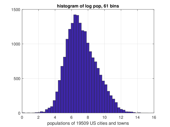
Figure 1: Populations Histogram

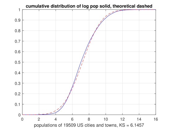
Figure 2: Populations Cumulative

5 Earthquake Time Model

Figure 3 displays a histogram of the natural logarithm of times between earthquake data. It appears be reflected Gumbel distributed so we modeled the data as random samples of a random variable $X$ such that $\ln X$ has density

$$p(x)=\frac{1}{\beta}\exp(z-e^{z}),\ z=\frac{x+\mu}{\beta}$$ (20)

where $\mu\in\mathbb{R}$ and $\beta>0.$ Its standard deviation equals $\pi\beta/\sqrt{6}$ and its mean equals $\mu-\beta\gamma$ where $\gamma\approx 0.5772$ is the Euler-Mascheroni constant. Using our data mean $7.2170$ and standard deviation $1.3754$ for $\ln s$ gives $\beta=1.0724$ and $\mu=7.8360.$ To test our model we compared the cumulative distribution of $\ln s$ with the theoretic cumulative distribution of $\ln X$ in Figure 4 and computed the Kolmogorov-Smirnov statistic to have value $1.8058.$ Thus

$$\hbox{Prob }(KS\geq 1.8058)\approx 0.0015$$ (21)

which suggests rejecting the null hypothesis that the data was formed from independent random samples of a log reflected Gumbel distribution with the specified parameters. However, the rejection is far less compelling than for the population data. The distributions of earthquake times is far closer to the log reflected Gumbel distribution than the distribution of populations is to the lognormal distribution.

Moreover, for our log reflected Gumbel $R_{0.01}(X)=714$ compared to our empirical value $R_{0.01}(s)=629$ which is much closer than for the population data.

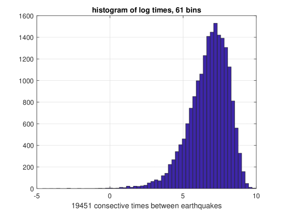
Figure 3: Earthquake Times Histogram

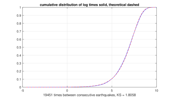
Figure 4: Earthquake Times Cumulative

Lemma 3

If $X$ is log reflected Gumbel distributed then it has a Weibull density

$$q(x)=\frac{k}{\lambda}\left(\frac{x}{\lambda}\right)^{k-1}e^{-(x/\lambda)^{k}}$$ (22)

where $\lambda=e^{-\mu}$ and $k=1/\beta.$

Proof: Equation (26) gives $p(x)=q(e^{x})e^{x}$ so the result follows from a direct computation.

Remark 3

Garavalia and colleagues [3] have modelled earthquake interoccurence times from an Italian database spanning 20 years, using Weibull distrbutions.

Lemma 4

The Weibel distribution is exponential iff $\beta=1$ otherwise it equals the following mixture of exponential distributions where $f$ is a uniquely determined probability density:

$$q(x)=\int_{0}^{\infty}yf(y)e^{-yx}dy.$$ (23)

Proof: Clearly $q(x)=-\frac{d}{dx}\mathcal{L}(f)(x)$ where $\mathcal{L}(f)$ is the Laplace transform of $f.$ Uniqueness follows since $\mathcal{L}(f)(0)=1$ and the fact that the Laplace transform is invertible.

Remark 4

Jewel [5] has used mixture of exponential distributions to study times of failure of units (patients, components) under observation. One can consider earthquakes as mechanical failures of geologic units in the Earth’s crust.

6 General Law for Random Variables

If $s$ consists of $n$ independent samples of an $\mathbb{R}_{+}$-valued random variable $X,$ then the law of large numbers ([2], Chapter VII, Lemma 1) implies that

$$\lim_{n\rightarrow\infty}Freq(R_{F,D}(s)=d)=Prob(R_{F,D}(X)=d),$$ (24)

with probability $1$ and hence

$$\lim_{n\rightarrow\infty}E_{F,D}(s)=E_{F,D}(X):=\sum_{d=1}^{D}\left[\,Prob(R_{F,D}(X)=d)-L_{F,D}(d)\,\right]^{2}.$$ (25)

This crucial fact motivates our additional consideration regarding random variables and their probabilities, besides sampled data and their frequencies. Henceforth in this section we assume that $X$ is a continuously distributed $\mathbb{R}_{+}$-valued randon variable with density $q:\mathbb{R}_{+}\mapsto[0,\infty).$ Then $\ln X$ is continuously distributed with density $p:\mathbb{R}\mapsto[0,\infty)$ given by

$$p(x)=\lim_{\Delta x\rightarrow 0}\frac{Prob(\ln X\in[x,x+\Delta x))}{\Delta x}=\lim_{\Delta x\rightarrow 0}\frac{Prob(X\in[e^{x},e^{x}e^{\Delta x}))}{\Delta x}=q(e^{x})e^{x}.$$ (26)

Define the $\ln F$-periodized function

$$\widetilde{p}(x):=\sum_{j\in\mathbb{Z}}p(x+j\ln F).$$ (27)

Clearly the restriction of $\widetilde{p}$ to the interval $[0,\ln F)$ is a probability density. Since

$$R_{F,D}(x)=d\hbox{ iff }\ln x\in I_{F,D}(d)+\mathbb{Z}\ln F,\ \ x\in\mathbb{R}_{+};\,d=1,...,D$$ (28)

where

$$I_{F,D}(d):=[\ln(1+(d-1)(F-1)/D),\ln(1+d(F-1)/D)),\ d=1,...,D,$$ (29)

it follows that

$$Prob(R_{F,D}(X)=d)=\int_{I_{F,D}(d)}\widetilde{p}(x)\,dx.$$ (30)

If $\widetilde{p}$ is constant then $\widetilde{p}=\frac{1}{\ln F},$

$$Prob(R_{F,D}(X)=d)=L_{F,D}(d),$$ (31)

and $E_{F,D}(X)=0$ for all integers $D\geq 2.$

Theorem 1

If $X$ is a $R_{+}$–valued continuously distributed random variable and $\ln X$ has density $p$ and $\widetilde{p}$ is defined by (27) then

$$DE_{F,D}(X)\leq(F-1)\int_{0}^{\ln F}e^{-x}\,\left[\widetilde{p}(x)-\frac{1}{\ln F}\right]^{2}\,dx.$$ (32)

If $D_{1}$ divides $D_{2}$ then

$$D_{1}\times E_{F,D_{1}}(X)\leq D_{2}\times E_{F,D_{2}}(X).$$ (33)

If $\widetilde{p}$ is Riemann integrable, then

$$\lim_{D\rightarrow\infty}DE_{F,D}(X)=(F-1)\int_{0}^{\ln F}e^{-x}\,\left[\widetilde{p}(x)-\frac{1}{\ln F}\right]^{2}\,dx.$$ (34)

Proof: (32) follows from the Schwarz inequality

$$\Bigg{|}\,Prob(R_{F,D}(X)=d)-L_{F,D}(d)\,\Bigg{|}^{2}=\Bigg{|}\int_{I_{F,D}(d)}\left(\widetilde{p}(x)-\frac{1}{\ln F}\right)\,e^{-x/2}\,e^{x/2}\,dx\,\Bigg{|}^{2}$$

$$\leq\int_{I_{F,D}(d)}e^{x}dx\,\int_{I_{F,D}(d)}\left(\widetilde{p}(x)-\frac{1}{\ln F}\right)^{2}e^{-x}\,dx=\frac{F-1}{D}\int_{I_{F,D}(d)}\left(\widetilde{p}(x)-\frac{1}{\ln F}\right)^{2}e^{-x}\,dx.$$

(33) follows from Lemma (2) and the law of large numbers (24). (34) follows from the definition of the Riemann integral and that fact that for large $D$ (11) gives $\hbox{ length }I_{F,D}(d)=L_{F,D}(d)\approx\frac{F-1}{D+d(F-1)},\ d=1,...,D.$

The periodized normal densities, also called the wrapped normal distributions, are well known to be expressed by the Jacobi theta function. Figures 5-8 show the plots of the $\l F$-periodicised functions $\widetilde{p}$ for $F=2,8,32,128$ where $p$ is a normal density with mean $7.2170$ and standard deviation $1.831$ corresponding to our model for the US populations.The max-min values of $\widetilde{p}$ increase rapidly with increasing $F$ but are extremely small for $F=2$ and $F=8.$

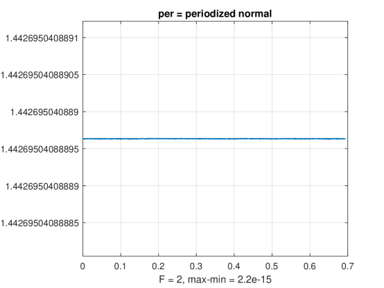
Figure 5: Periodized Normal Density

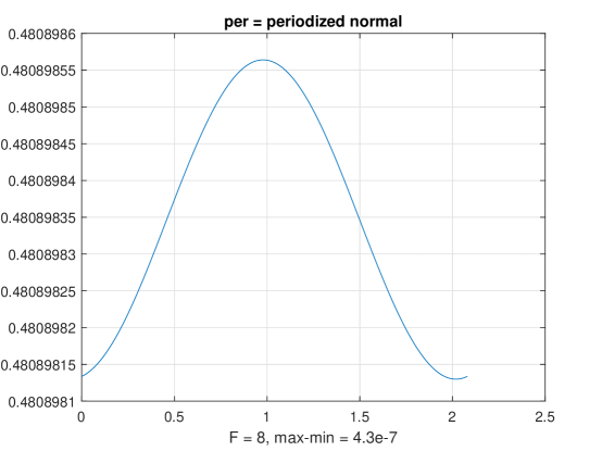
Figure 6: Periodized Normal Density

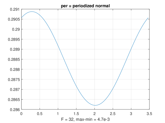
Figure 7: Periodized Normal Density

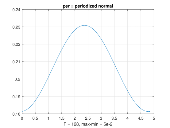
Figure 8: Periodized Normal Density

Definition 2

The Fourier transform of a density function $p:\mathbb{R}\mapsto[0,\infty)$ is the function $\widetilde{p}:\mathbb{R}\mapsto\mathbb{C}$ defined by $\widehat{p}(y):=\int_{\mathbb{R}}p(x)\,e^{-2\pi iyx}\,dx.$

Lemma 5

The normal density

$$p(x)=\frac{1}{\sigma\sqrt{2\pi}}\exp(-\frac{1}{2\sigma^{2}}(x-\mu)^{2})$$

has Fourier transform

$$\widehat{p}(y)=\exp(-2\pi i\mu y)\,\exp(-2\pi^{2}\sigma^{2}y)$$

which never vanishes. The reflected Gumbel density

$$p(x)=\frac{1}{\beta}\exp(z-e^{z}),\ z=\frac{x+\mu}{\beta}$$

has Fourier transform

$$\widehat{p}(y)=e^{2\pi i\mu y}\,\Gamma(1-2\pi i\beta y).$$ (35)

which never vanishes.

Proof: The Fourier transform of the normal density is computed by completing the square and then replacing the contour of integration $\mathbb{R}$ by a contour $\mathbb{R}+2\pi i\sigma.$ For the reflected Gumbel density $\widehat{p}(y):=\int_{\mathbb{R}}p(x)\,e^{-2\pi iyx}\,dx=e^{2\pi i\beta\mu y}\int_{\mathbb{R}}\exp(z-e^{z})\,e^{-2\pi i\beta zy}\,dz$
$=e^{2\pi iy\ln\mu}\int_{0}^{\infty}e^{-u}\,u^{(1-2\pi iy)-1}du=e^{2\pi iy\ln\mu}\Gamma(1-2\pi i\beta y).$ The Gamma function never vanishes since it satisfies the well known identity

$$\Gamma(z)\,\Gamma(1=z)=\frac{\pi}{\sin\pi z},\ \ z\in\mathbb{C}.$$

Lemma 6

Fourier Inversion Theorem: If $f:\mathbb{R}\rightarrow\mathbb{C}$ is integrable and sufficiently smooth and $h(x):=\int_{\mathbb{R}}f(x)\,e^{2\pi iyx}\,dy,$ then $\widehat{h}=f.$

Proof: See ([2], p. 509-510).

Lemma 7

$\widetilde{p}=\frac{1}{\ln F}$ is constant iff the Fourier transform satisfies

$$\widehat{p}(j/\ln F)=0,\ \ j\in\mathbb{Z}\backslash\{0\}.$$ (36)

Proof: $\widetilde{p}$ has periodic $1/\ln F$ so has a Fourier series expansion $\widehat{p}(x)=\sum_{k\in\mathbb{Z}}c_{k}\,e^{2\pi ikx/\ln F}$ with $c_{k}=\frac{1}{\ln F}\int_{[0,\ln F)}\widehat{p}(x)e^{-2\pi ikx/\ln F}.$ Substituting (27) into this expression gives

$$c_{k}=\int_{[0,\ln F)}\sum_{j\in\mathbb{Z}}p(x+j\ln F)e^{-2\pi ikx/\ln F}\,dx$$

$$=\int_{[0,\ln F)}\sum_{j\in\mathbb{Z}}p(x+j\ln F)e^{-2\pi ik(x+j\ln F)/\ln F}\,dx$$

$$=\sum_{j\in\mathbb{Z}}\int_{[0,\ln F)+j\ln F}p(x+j\ln F)e^{-2\pi ik(x+j\ln F)/\ln F}\,dx$$

$$=\int_{\mathbb{R}}p(x)e^{-2\pi ikx/\ln F}\,dx=\widehat{p}(k/\ln F),\ \ k\in\mathbb{Z}.$$

Definition 3

A random variable $X$ is $F$-perfect if $E_{F,D}(X)=0$ for every integer $D\geq 2.$

The following is a slight generalization of ”Benford’s law compliance theorem” derived by Steven Smith ([13], p. 716).

Lemma 8

For a continuously distributed random variable $X$ let $p$ be the density function of $\ln X$ and let $F>1.$ Then $X$ is $F$-perfect iff $\widehat{p}(j/\ln F)=0$ for every nonzero integer $j.$

Proof: Follows directly from Equation (34) in Theorem 1 (34) and from Lemma 7.

Theorem 2

No random variable is $F_{j}$-perfect for every $F_{j}$ if $F_{j}\rightarrow\infty.$ For every $K>0$ there exists a random variable $X$ that is $F$-perfect whenever $\ln F\leq 1/K.$ Lognormal and log reflected Gumbel distributed random variables are never $F$-perfect.

Proof: If $X$ is $F_{j}$-perfect for every $j$ then $\widehat{p}(0)=\lim_{j\rightarrow\infty}\widehat{p}(1/\ln F_{j})=0$ but this contradicts the fact that $\widehat{p}(0)=\int_{\mathbb{R}}p(x)dx=1.$ To prove the second assertion define

$$h(x):=\begin{cases}\frac{1}{\sqrt{K}}\hbox{ if }x\in[-K/2,K/2]\\ 0\hbox{ otherwise}.\end{cases}$$

and the convolution

$$f(x):=\int_{\mathbb{R}}h(x-y)h(y)dy=\begin{cases}1+x/K\hbox{ if }x\in[-K,0]\\ 1-x/K\hbox{ if }x\in[0,K]\\ 0\hbox{ otherwise}.\end{cases}$$

Then define

$$p(x):=\int_{\mathbb{R}}f(y)e^{2\pi iyx}\,dy=\bigg{|}\int_{\mathbb{R}}h(y)e^{2\pi iyx}\,dy\bigg{|}^{2}=\frac{1}{K}\left(\frac{\sin(\pi Kx)}{\pi x}\right)^{2}.$$

Lemma 6 implies that $\widehat{p}=f$ so $\widehat{p}(j/\ln F)=0$ for $j\in\mathbb{Z}\backslash\{0\}$ and $\ln F\leq 1/K.$ Let $X$ be a random variable such that the density of $\ln X$ equals $p.$ The assertions about lognormal and log reflected Gumbel distributions follow from Lemmas 5 and 8

The three tables below display values of $L_{F,5}(d),F=2,8,32;d=1,...,5$ and the Prob$(R_{F,D}(X)=d),F=2,8,32;d=1,...,5$ for the lognormal and log reflected Gumbel distributed random variable $X$ whose parameters were chosen to equal those for US populations and times between successive earthquakes. These were the probability models discussed in Sections 4 and 5. The last columns contain the sum of squared errors.

$$\begin{array}[]{ccccccc}L_{2,5}&0.26303441&0.22239242&0.19264508&0.16992500&0.15200309&0\\ lognormal&0.26303441&0.22239242&0.19264508&0.16992500&0.15200309&1.1e-28\\ logGumbel&0.26303431&0.22239316&0.19264535&0.16992461&0.15200257&1.1e-12\end{array}$$

$$\begin{array}[]{ccccccc}L_{8,5}&0.42101147&0.22098834&0.15083740&0.11465147&0.09251133&0\\ lognormal&0.42099290&0.22116695&0.15084018&0.11457438&0.09242559&4.6e-8\\ logGumbel&0.42311092&0.21018579&0.15025476&0.11896115&0.09748739&1.6e-4\end{array}$$

$$\begin{array}[]{ccccccc}L_{32,5}&0.56959938&0.17923284&0.10972413&0.07930348&0.06214017&0\\ lognormal&0.58122693&0.16012001&0.10727135&0.08330820&0.06807350&5.6e-4\\ logGumbel&0.67229291&0.13437162&0.07473944&0.06235662&0.05623941&1.4e-2\end{array}$$

Remark 5

Comparing these tables with the tables for natural data sequences shows that probability densities may better approximate the generalized law than the frequencies of natural data that they model. This may be useful for density estimation that is a crucial tool in statistical pattern recognition, machine intelligence, and data science.

7 Appendix 1: Kossovsky’s Partition

In ([7], Section 7, Chapters 122 and 123) Kossovsky partioned positive numbers as

$$\mathbb{R}_{+}=(0,w)\cup\bigcup_{d=1}^{D}\bigcup_{j=0}^{\infty}[1+(d-1)(F-1)/D,1+d(F-1)/D)wF^{j}$$ (37)

where $w>0$ is extremely small. Since $w=F^{L}c$ where $c\in[1,F)$ and the integer $L<<0$ are unique, we get

$$\mathbb{R}_{+}=(0,F^{L}c)\cup\bigcup_{d=1}^{D}\bigcup_{j=L}^{\infty}[1+(d-1)(F-1)/D,1+d(F-1)/D)F^{j}c.$$ (38)

Taking the limit as $w\rightarrow 0$ gives $L\rightarrow-\infty$ hence

$$\mathbb{R}_{+}=\bigcup_{d=1}^{D}c\Sigma_{F,D}(d)$$ (39)

where $\Sigma_{F,D}(d)$ is defined in (3). So this corresponds to scaling the data by the factor $1/c$ which does not effect the Benford compliance of the data. However, for $F=D+1,$ and $x>0,$ $x\in c\Sigma_{F,D}(d)$ iff the first digit of the base $F$ representation of $x/c$ equals $d.$

In ([7], Section 7, Chapters 124-129) Kossovsky used his partition (37) to initially define

$$L_{F,D}(d):=\lim_{L\rightarrow\infty}Prob(R_{F,D}(X_{w,L})=d),\ d=1,...,D$$ (40)

where $X_{w,L}$ is the random variable with density $k/x$ on $[w,L]$ and $k=1/\ln(L/w).$ He derived an expression for $Prob(R_{F,D}(X_{w,L})=d),d=1,...,D$ as the ratio of two quantities both converging to $\infty.$ George Andrews proved that its limit equals the expression for $L_{F,D}(d)$ in (7).

8 Appendix 2: MATLAB Programs

function [GLvals,LFD,Diff,EFD] = GLnorm(F,D,mu,sigma)
Inputs and Outputs
F : base
D : number of bins
mu : mean of normal density
sigma : standard deviation of normal density
LFD : ideal GL values
GLvals : actual GL values
Start of Algorithm
r = 0:D; r = 1+r*(F-1)/D; r = log(r);
LFD = (r(2:D+1)-r(1:D))/log(F);
M = zeros(21,D+1);
LF = log(F);
for j = 1:101
M(j,1:(D+1)) = r + (j-51)*LF;
end
M = (M-mu)/sigma;
s = sign(M);
eM = 0.5+0.5*s.*erf(s.*M);
reM = sum(eM);
GLvals = reM(2:D+1)-reM(1:D);
Diff = GLvals-LFD;
EFD = Diff*Diff’;
end

function [GLvals,LFD,Diff,EFD] = GLGumbel(F,D,mu,beta)
Inputs and Outputs
F : base
D : number of bins
mu : mode (max argument) (= mean + beta*gamma)
beta : (= sigma*sqrt(6)//pi)
density(x) = (1/beta)*exp[w - exp(w)], w = (x-mu)/beta
LFD : ideal GL values
GLvals : actual GL values
Start of Algorithm
r = 0:D; r = 1+r*(F-1)/D; r = log(r);
LFD = (r(2:D+1)-r(1:D))/log(F);
M = zeros(21,D+1);
LF = log(F);
for j = 1:101
M(j,1:(D+1)) = r + (j-51)*LF;
end
M = (M-mu)/beta;
cM = 1-exp(-exp(M));
rcM = sum(cM);
GLvals = rcM(2:D+1)-rcM(1:D);
Diff = GLvals-LFD;
EFD = Diff*Diff’;
end

function [x,per,mm] = periodizednormal(sigma,m,F)
period = log(F);N = 10000;dx = period/N; dy = period/(N-1);x = 0:dy:period;
a= -0.5/sigma²; b = 1/(sigma*sqrt(2*pi)); J = size(x,2);
K1 = round(m-50*sigma); K2 = round(m+50*sigma); y = x-m;
for j = 1:J
per(j) = 0;
for k = K1:K2
d = b*exp(a*(y(j)-k*period)²);
per(j) = per(j)+d;
end
end
plot(x,per)
title(’per = periodized normal’)
grid
mm = max(per)-min(per);
end

Acknowledgment We thank the distinguished mathematician George Andrews for his ingenious proof which enabled the entire discussion of this article. Andrews is well known for his discovery of Ramanujan’s lost notebook at Trinity College’s library, Cambridge in 1976, and for his extensive work on Ramanujan’s research. Andrews stated recently that his computation of the expression for $L_{F,D}$ in the GLORQ was inspired by this work. Accordingly both authors indirectly owe gratitude to Ramanujan of India as well.

References

- [1] F. Benford, The law of anomalous numbers, Proceedings of the American Philosophical Society 78 (1938) 551-572.
- [2] W. Feller, An Introduction to Probability Theory and Its Applications, vol. 2, 1st edition, John Wiley, New York, 1971.
- [3] E. Garavaglia, E. Guagenti, R. Pavani, L. Petrini, Renewal models for earthquake predictability, J. Seismology 14 (1) (2010) 79-93. doi:10.1007/s10950-008-9147-6
- [4] E. J. Gumbel, Les valeurs extrêmes des distributions statistique, Annales de l’Institute Henri Poincaré 5 (2) (1935) 115-158.
- [5] N. P. Jewel, Mixtures of exponential distributions, The Annals of Statistics 10 (2) (1982) 479-484.
- [6] A. E. Kossovsky, On the relative quantities occurring within physical data sets, May 8, 2013. arxiv.org/abs/1305.1893
- [7] A. E. Kossovsky, Benford’s Law: Theory, the General Law of Relative Quantities, and Forensic Fraud Detection Applications, World Scientific Publishing Company. August 2014. ISBN: 978-9814651202
- [8] A. E. Kossovsky, Small is Beautiful: Why the Small is Numerous but the Big is Rare in the World, Kindle Direct Publishing, June 2017. ISBN 978-0692912416
- [9] A. E. Kossovsky, Studies in Benford’s Law: Arithmetical Tugs of War, Quantitative Partition Models, Prime Numbers, Exponential Growth Series, and Data Forensics, Kindle Direct Publishing, April 2019. ISBN 978-1729283257
- [10] E. Kouassi, E. Akpata, K. Pokou, A note on Lapalace transforms of some common distributions used in counting processes analysis, Applied Mathematics 11 (2020) 67-75. doi.org/10.4236/am.2020.112007
- [11] S. Newcomb, Note on the frequency of use of the different digits in natural numbers, American Journal of Mathematics 4 (1/4) (1881) 39-40. doi:10.2307/2369148
- [12] W. Rudin, Principles of Mathematical Analysis, 3rd Edition, McGraw-Hill, New York, 1964.
- [13] S. W. Smith, Chapter 34: Explaining Benford’s Law. The Power of Signal Processing, The Scientist and Engineer’s Guide to Digital Signal Processing. Retrieved 15 December 2012. http://www.dspguide.com/ch34/5.htm