The algebraic degree of sparse polynomial optimization

Abstract.

In this paper we study a broad class of polynomial optimization problems whose constraints and objective functions exhibit sparsity patterns. We give two characterizations of the number of critical points to these problems, one as a mixed volume and one as an intersection product on a toric variety. As a corollary, we obtain a convex geometric interpretation of polar degrees, a classical invariant of algebraic varieties as well as Euclidean distance degrees. Furthermore, we prove BKK generality of Lagrange systems in many instances. Motivated by our result expressing the algebraic degree of sparse polynomial optimisation problems via Porteus’ formula, in the appendix we answer a related question concerning the degree of sparse determinantal varieties.

Keywords: sparse polynomial optimization, toric varieties, algebraic degree, ED degree, polar degree

MSC2020: 90C26, 14M25, 14Q20, 52B20

1. Introduction

We consider a polynomial optimization problems of the form:

(POP) $$\min_{x\in\mathbb{R}^{n}}\ f_{0}(x)\quad\text{subject to}\quad f_{1}(x)=0,\ldots,f_{m}(x)=0$$

where $f_{i}\in\mathbb{R}[x_{1},\ldots,x_{n}]$. Polynomial optimization problems have broad modelling power and have found applications in signal processing, combinatorial optimization, power systems engineering and more [TR01, PRW95, MH19]. In general these problems are NP hard to solve [Vav90] but there has been much work in the recent decades studying various solution techniques for (POP). Inspired by recent increases in performance of numerical polynomial system solving, in this work we focus on solving critical point equations.

When the first order optimality conditions hold, there are finitely many complex critical points to (POP). For a specified objective function $f_{0}$ and fixed constraints $f_{1},\ldots,f_{m}$ we denote $\mathbf{F}=(f_{0},\ldots,f_{m})$. The number of complex critical points of $\mathbf{F}$ is called the algebraic degree of $\mathbf{F}$. While (POP) is a real optimization problem, one considers the number of complex critical points since for polynomials $\mathbf{F}$ with fixed monomial support, the algebraic degree is generically constant. Further, when the first order optimality conditions of (POP) hold, then the coordinates of the optimal solution of (POP) are algebraic functions of the coefficients of $\mathbf{F}$.

The algebraic degree of $\mathbf{F}$ has an additional interpretation as the degree of these algebraic functions. Observe also that the algebraic degree gives an upper bound on the number of critical points of (POP). This gives a bound on how many places local optimization methods can get caught at non-optimal critical points.

A formula for the algebraic degree when $\mathbf{F}$ consist of generic polynomials with full monomial support was given in [NR09a]. This was then specialized for many classes of convex polynomial optimization problems in [GvBR09] and [NRS10]. When the objective function is the Euclidean distance function, i.e. $f_{0}=\lVert x-u\rVert_{2}^{2}$ for a point $u\in\mathbb{R}^{n}$, the number of critical points to (POP) for general $u$ is called the ED degree of $(f_{1},\ldots,f_{m})$. The study of ED degrees began with [DHO⁺14] and initial bounds on the ED degree of a variety was given in [DHO⁺16]. Other work has found the ED degree for real algebraic groups [BD15], Fermat hypersurfaces [Lee17], orthogonally invariant matrices [DLOT17], smooth complex projective varieties [AH18], the multiview variety [MRW20a], when $m=1$ [BSW21] and when the data $u$ and polynomials $f_{1},\ldots,f_{m}$ are not general [MRW20b].

A related problem considers maximum likelihood estimation which considers the objective function $f_{0}=x_{1}^{u_{1}}\cdots x_{n}^{u_{n}}$. The number of complex critical points is called the ML degree of $(f_{1},\ldots,f_{m})$. Relationships between ML degrees and Euler characteristics as well as the ML degree of various statistical models have been studied in [CHKS06, HKS05, Huh13, ABB⁺19, DM21, MMW21, MMM⁺23].

Inspired by recent results on the ED and ML degrees of sparse polynomial systems [BSW21, LNRW23], we study the algebraic degree of (POP) when each $f_{i}\in\mathbb{R}[x_{1},\ldots,x_{n}]$ is assumed to be a sparse polynomial with generic coefficients. Given an optimization problem of the form (POP) where $\mathbf{F}$ is a general list of sparse polynomial equations, define the Lagrangian of $\mathbf{F}$ to be

$$\Phi_{F}(\lambda,x):=f_{0}-\sum_{i=1}^{m}\lambda_{i}f_{i}.$$

We consider the Lagrange system of $\mathbf{F}$, $\mathbf{L}_{\mathrm{F}}=(f_{1},\ldots,f_{m},\ell_{1},\ldots,\ell_{n})$ where

$$\ell_{j}=\frac{\partial}{\partial x_{j}}\left(f_{0}-\sum_{i=1}^{m}\lambda_{i}f_{i}\right).$$

Analogous to the algebraic degree of polynomial optimization from [NR09b] we generalize the term to the algebraic degree of sparse polynomial optimization. It denotes the number of critical points:

(1.1) $$\#\mathcal{V}\left(\mathbf{L}_{\mathrm{F}}\right)=\#\left\{(x,\lambda)\in\mathbb{C}^{n}\times\mathbb{C}^{m}:\quad 0=f_{1}=\cdots=f_{m}=\ell_{1}=\cdots=\ell_{n}\right\}$$

of $f_{0}$ restricted to $\mathcal{V}(f_{1},\ldots,f_{m})$ where each $f_{i}\in\mathbb{R}[x_{1},\ldots,x_{n}]$ is a sparse polynomial.

There exist classical results in algebraic geometry bounding the number of isolated solutions to a square polynomial system. A result of Bezout says that $\#\mathcal{V}(\mathbf{L}_{\mathrm{F}})$ is bounded above by the product of the degrees of the polynomials in $\mathbf{L}_{\mathrm{F}}$. If $\deg(f_{i})=d_{i}$ and $\deg(\ell_{j})=c_{j}$, $0\leq i\leq m,1\leq j\leq n$, Bezout’s bound reduces to $d_{1}\cdots d_{m}\cdot c_{1}\cdots c_{n}$ where $c_{j}\leq\max_{i\in[m]}\{d_{0}-1,d_{i}\}$. The work of Nie and Ranestad refined this bound considerably and showed that

$$\#\mathcal{V}(\mathbf{L}_{\mathrm{F}})\leq d_{1}\cdots d_{m}\cdot D_{n-m}(d_{0}-1,\ldots,d_{m}-1)$$

where $D_{r}(n_{1},\ldots,n_{k})=\sum_{i_{1}+\cdots+i_{k}=r}n_{1}^{i_{1}}\cdots n_{k}^{i_{k}}$ is the symmetric sum of products [NR09a]. While this bound is generically tight for dense polynomial systems, the following example shows that it can quite bad (even worse than Bezout’s bound) for sparse polynomial systems.

Example 1.1.

Consider the following optimization problem:

(1.2) $$\min_{x\in\mathbb{R}^{n}}\ c^{T}x\quad\text{subject to}\quad f=\alpha_{1}x_{1}^{3}+\sum_{j=2}^{n-1}\alpha_{j}x_{j}^{2}+\alpha_{n}x_{n}=1.$$

where $c,\alpha\in\mathbb{R}^{n}$ are generic parameters. The corresponding Lagrange system is given by $\mathbf{L}_{\mathrm{F}}=(\ell_{1},\ldots,\ell_{n},f)$ where

$$\ell_{1}=c_{1}-3\lambda\alpha_{1}x_{1}^{2},\quad\ell_{n}=c_{n}-\alpha_{n}\lambda,\quad\ell_{j}=c_{i}-2\lambda\alpha_{j}x_{j},\ 2\leq j\leq n-1.$$

The Bezout bound tells us that $\#\mathcal{V}(\mathbf{L}_{\mathrm{F}}))\leq 3\cdot 2^{n-2}$ which is better than the Nie-Ranestad bound which gives $\#\mathcal{V}(\mathbf{L}_{\mathrm{F}}))\leq 3\cdot D_{n-1}(0,2)=3\cdot 2^{n-1}$. In this case, the sparsity of the Lagrange equations allows one to solve the system by hand one variable at a time and therefore can see that for generic $c,\alpha$, $\#\mathcal{V}(\mathbf{L}_{\mathrm{F}})=2$.

This work is motivated by the previous example and proves stronger bounds for the algebraic degree of sparse polynomial optimization programs. This paper focuses on the following question.

Question 1.

How many smooth critical points does (POP) have for sparse $\mathbf{F}$?

The motivation for 1 is that if we know how many critical points (POP) has, and we find them all, then we can globally solve (POP). The only way to provably find all smooth critical points is to find all complex solutions of $\mathbf{L}_{\mathrm{F}}$.

The field of computational algebraic geometry has traditionally been associated with symbolic computations based on Gröbner bases. Recent developments in numerical frameworks, such as homotopy continuation [BSHW13], provide algorithms that are able to solve problems intractable with symbolic methods. Moreover, numerical algorithms can not only provide the floating point approximation of a solution, but also certify that a given approximation represents a unique solution, and provide guarantees for correctness [BRT23, Rum99, Lee19]. Therefore, numerical computation can be used to prove lower bounds to the number of solutions. However, to guarantee that there are no other roots, one needs an upper bound to $\#\mathcal{V}(\mathbf{L}_{\mathrm{F}})$, which can be obtained using intersection theory.

Such an intersection theoretic bound for sparse polynomial systems was given by the celebrated Bernstein-Kouchnirenko-Khovanskii (BKK) theorem. BKK theorem relates the number of isolated $\mathbb{C}^{*}$ zeros to a system of polynomial equations to the mixed volume of the corresponding Newton polytopes (see Section 2.1). While their bound is generically tight, we note that the coefficients of the system $\mathbf{L}_{\mathrm{F}}$ are linearly dependent, so a priori it is not clear that the system $\mathbf{L}_{\mathrm{F}}$ is BKK general. This inspires the second question motivating this work.

Question 2.

Is the Lagrange system of (POP) BKK general?

An affirmative answer to 2 would show that polyhedral homotopy algorithms are optimal for finding all complex critical points to (POP) in the sense that for every solution to $\mathbf{L}_{\mathrm{F}}=0$, exactly one homotopy path is tracked. For more details on polyhedral homotopy continuation see [HS95]. Furthermore, understanding BKK exactness of non generic polynomial systems is of increasing interest in the applied algebraic geometry community.

A final consequence of 2 has to do with the complexity of algorithms in real algebraic geometry. A fundamental question in real algebraic geometry is to find a point on each connected component of a real algebraic variety, $X$. In [Hau13], it was shown that when $f_{0}$ is the Euclidean distance function, the zeros of the Lagrange system of $f_{0}$ restricted to $X$ cover all connected components. By showing that polyhedral homotopy algorithms are optimal for a large class of Euclidean distance optimization problems we would then reduce the complexity of the algorithm given in [Hau13, Section 2.1] since we don’t need to worry about homotopy paths diverging.

Contribution

Our contribution is several results based on intersection theory that determine the number of critical points of generic, sparse polynomial programs. First, we show in B, the answer to 2 is positive for a wide class of sparse polynomial programs having strongly admissible monomial support (see Definition 3.4). In particular, our results show that the bound is tight for Example 1.1.

As a corollary, we generalize the result in [BSW21] in this case and show that the ED degree of a variety with strongly admissible support is equal to the BKK bound of its corresponding Lagrange system (4.1). We also prove analogous results for (the sum of) polar degrees (4.5), giving the first convex geometric interpretation of the algebraic invariant. Further, in 3.7 we show that algebraic degrees of generic sparse polynomial programs are determined by the Newton polytopes of $\mathbf{F}$. 3.7 has also algorithmic implications which were studied in [LMR23].

For a larger family of sparse polynomial programs, in C we provide a different formula for the corresponding algebraic degrees. Our main tool here is Porteus’ formula which computes the fundamental class of the degeneracy locus of a morphism between two vector bundles as a polynomial in their Chern classes. Using Porteus’ formula C expresses the algebraic degree in terms of the intersection theory of certain toric compactification of $(\mathbb{C}^{*})^{n}$. The formula for algebraic degree in C can be expressed as a (non-necessarily positive) linear combination of mixed volumes. However, the explicit connection to the mixed volume of Lagrange system is still mysterious.

Finally, in Appendix A we study a closely related problem of computing degrees of sparse determinantal varieties. Our main result here is Theorem A.2 which computes these degrees as the mixed volume of certain polytopes. To obtain this result we prove a toric version of Porteus’ formula.

2. Preliminaries and notation

2.1. Sparse polynomials and polyhedral geometry

A sparse polynomial $f\in\mathbb{C}[x_{1},\ldots,x_{n}]$ is defined by its monomial support and its coefficients. Specifically, for a subset $\mathcal{A}\subset\mathbb{N}^{n}=\mathbb{Z}_{\geq 0}^{n}$, we write

$$f=\sum_{\alpha\in\mathcal{A}}c_{\alpha}x^{\alpha}$$

where $x^{\alpha}:=x_{1}^{\alpha_{1}}\cdots x_{n}^{\alpha_{n}}$ and $c_{\alpha}\in\mathbb{C}$. For a sparse polynomial $f$, we associate to it a polytope called the Newton polytope of $f$ which is defined as the convex hull of its exponent vectors. It is denoted ${\mathrm{Newt}}(f)=\operatorname{conv}\{\alpha\ :\ \alpha\in\mathcal{A}\}$. A sparse polynomial system $\mathbf{F}=(f_{0},\ldots,f_{m})$ is then defined by a tuple $\mathcal{A}=(\mathcal{A}_{0},\ldots,\mathcal{A}_{m})$ where $f_{i}=\sum_{\alpha\in\mathcal{A}_{i}}c_{\alpha,i}x^{\alpha}\in\mathbb{C}[x_{1},\ldots,x_{n}]$.

Remark 2.1.

In this paper we consider generic sparse polynomial systems. A statement holds for a generic sparse polynomial system if it holds for all systems $\mathbf{F}$ where for each $i=0,\dots,m$ the coefficients $\{c_{\alpha,i}\}_{\alpha\in\mathcal{A}_{i}}$ of $f_{i}$ lie in some nonempty Zariski open subset of the space $\mathbb{C}^{\mathcal{A}_{0}}\times\cdots\times\mathbb{C}^{\mathcal{A}_{m}}$ of coefficients. This means that the non-generic behavior occurs on a set of measure zero in the space $\mathbb{C}^{\mathcal{A}_{0}}\times\cdots\times\mathbb{C}^{\mathcal{A}_{m}}$.

Given polytopes $P_{1},\ldots,P_{n}\in\mathbb{R}^{n}$, the mixed volume of $P_{1},\ldots,P_{n}$ is the coefficient in front of the monomial $\lambda_{1}\cdots\lambda_{n}$ of the polynomial

$${\mathrm{Vol}}_{n}(\lambda_{1}P_{1}+\ldots+\lambda_{n}P_{n})$$

where $P+Q=\{p+q\ :\ p\in P,\ q\in Q\}$ is the Mikowski sum and ${\mathrm{Vol}}_{n}$ is the standard $n$-dimensional Euclidean volume.

In a series of celebrated results [Ber75, Kou76, Kho78] the connection between the number of $\mathbb{C}^{*}:=\mathbb{C}\backslash\{0\}$ solutions to a system of sparse polynomial equations and the underlying convex geometry of the polynomials was made.

Theorem 2.2 (BKK Bound [Ber75, Kou76, Kho78]).

Let $\mathbf{F}=(f_{1},\ldots,f_{n})\subset\mathbb{C}[x_{1},\ldots,x_{n}]$ be a sparse polynomial system with $\eta$ isolated $\mathbb{C}^{*}$ solutions counted with multiplicity and let $P_{i}={\mathrm{Newt}}(f_{i})$. Then

$$\eta\leq{\mathrm{MV}}(P_{1},\ldots,P_{n}).$$

Moreover, if the coefficients of $\mathbf{F}$ are general then $\eta={\mathrm{MV}}(P_{1},\ldots,P_{n})$.

If for a sparse polynomial system $\mathbf{F}$ the BKK bound holds with equality, we say $\mathbf{F}$ is BKK general. Bernstein gave explicit degeneracy conditions under which the above inequality is tight by considering the initial systems of $\mathbf{F}$ [Ber75].

Given a polytope $P\subset\mathbb{R}^{n}$ and a vector $w\in\mathbb{Z}^{n}\backslash\{0\}$, let $P_{w}$ denote the face exposed by $w$. Specifically,

$$P_{w}=\{x\in P\ :\ \langle x,w\rangle\leq\langle y,w\rangle\ \forall y\in P\}.$$

For a sparse polynomial $f$ we call

$${\mathrm{init}}_{w}(f)=\sum_{\alpha\in({\mathrm{Newt}}(f))_{w}}c_{\alpha}x^{\alpha}$$

the initial polynomial of $f$ with respect to $w$. For a sparse polynomial system $\mathbf{F}$, we denote ${\mathrm{init}}_{w}(\mathbf{F})=({\mathrm{init}}_{w}(f_{1}),\ldots,{\mathrm{init}}_{w}(f_{n}))$.

Theorem 2.3.

[Ber75, Theorem 2] Let $\mathbf{F}=(f_{1},\ldots,f_{n})\subset\mathbb{C}[x_{1},\ldots,x_{n}]$ be a sparse polynomial system with $\eta$ isolated $\mathbb{C}^{*}$ solutions counted with multiplicity and let $P_{i}={\mathrm{Newt}}(f_{i})$. All $\mathbb{C}^{*}$ solutions of $F(x)=0$ are isolated and $\eta={\mathrm{MV}}(P_{1},\ldots,P_{n})$ if and only if for every $w\in\mathbb{Z}^{n}\backslash\{0\}$, ${\mathrm{init}}_{w}(\mathbf{F})$ has no $\mathbb{C}^{*}$ solutions.

Theorem 2.2 and Theorem 2.3 demonstrate the intimate connection between solutions to systems of polynomial equations and polyhedral geometry. In the remainder of this section we define a few more objects that are helpful when using this connection. Given $\mathcal{A}=(\mathcal{A}_{0},\ldots,\mathcal{A}_{m})\in\mathbb{N}^{n}$ we define the Cayley polytope of $\mathcal{A}$ as

$${\mathrm{Cay}}(\mathcal{A})=\operatorname{conv}\left(\{(x,e_{i})\ :x\in\mathcal{A}_{i},i=0,\dots,m\}\right)\subset\mathbb{R}^{n+m}$$

where $e_{i}$ is the $i$th standard basis vector of $\mathbb{R}^{m}$ and $e_{0}$ is the vector of all zeroes. Similarly, for a sparse polynomial system $\mathbf{F}$, with support $\mathcal{A}=(\mathcal{A}_{0},\ldots,\mathcal{A}_{m})$ we define ${\mathrm{Cay}}(\mathbf{F})={\mathrm{Cay}}(\mathcal{A})$.

For a face of a convex polytope, $F\subset P\subset\mathbb{R}^{n}$, the normal cone of $F$ is the set of linear functionals which achieve their minimum on $F$, i.e.

$$\sigma(F)=\{c\in\mathbb{R}^{n}\ :\ \langle c,x\rangle\leq\langle c,y\rangle,\ \forall x\in F,\ y\in P\}.$$

The normal cones of each face of $P$ form a fan, denoted ${\Sigma}(P)\subset\mathbb{R}^{n}$.

Finally, throughout the rest of this paper we will consider the operation of taking the “partial derivative” of a polytope which we define as follows. Let $P\subset\mathbb{R}_{\geq 0}^{n}$ be a polytope contained in the positive orthant. Then

$$\partial_{j}P=(P-e_{j})\cap\mathbb{R}_{\geq 0}^{n}=\{\alpha-e_{j}\ :\ \alpha\in P,\ \alpha_{j}\geq 1\},$$

where $e_{j}$ is the standard basis vector of $\mathbb{R}^{n}$.

Of course, the definition of $\partial_{j}P$ is motivated by the partial differentiation operation of a polynomial $f\in\mathbb{R}[x_{1},\ldots,x_{n}]$ with ${\mathrm{Newt}}(f)=P$. Indeed, one always has ${\mathrm{Newt}}(\frac{\partial}{\partial x_{j}}f)\subset\partial_{j}{\mathrm{Newt}}(f)$. However, ${\mathrm{Newt}}(\frac{\partial}{\partial x_{j}}f)$ and $\partial_{j}{\mathrm{Newt}}(f)$ can be quite different. For instance, let $f(x)=1+x^{3}$, then ${\mathrm{Newt}}(f)=[0,3]$ and $\partial{\mathrm{Newt}}(f)=[0,2]$. However, $\frac{\partial}{\partial x}f=3x^{2}$ and ${\mathrm{Newt}}(\frac{\partial}{\partial x}f)=\{2\}$. In general, even if $P$ is integral, the polytope $\partial_{i}P$ does not have to be integral.

For a polynomial $f=\sum_{\alpha\in\mathcal{A}}c_{\alpha}x^{\alpha}$ having full monomial support (i.e. $c_{\alpha}\neq 0$ for any $\alpha\in{\mathrm{Newt}}(f)\cap\mathbb{N}^{n}$) the two constructions are connected in the following way:

$${\mathrm{Newt}}\left(\frac{\partial}{\partial x_{j}}f\right)=\operatorname{conv}\{\partial_{j}{\mathrm{Newt}}(f)\cap\mathbb{N}^{n}\}.$$

In particular, if $f$ is a degree $d$ polynomial with all monomials of degree $\leq d$ having non-zero coefficients, then

$${\mathrm{Newt}}\left(\frac{\partial}{\partial x_{j}}f\right)=\partial_{j}{\mathrm{Newt}}(f).$$

2.2. Toric varieties

Theorem 2.2 can be seen as an intersection theory question on toric varieties. A toric variety $X$ is an irreducible variety such that $(\mathbb{C}^{*})^{n}$ is a Zariski open subset of $X$ and the action of $(\mathbb{C}^{*})^{n}$ on itself extends to an action of $(\mathbb{C}^{*})^{n}$ on $X$. We can also associate toric varieties to polyhedral fans.

Let $\sigma\in\mathbb{R}^{n}$ be a rational polyhedral cone which does not contain any vector subspace and denote

$$S_{\sigma}=\sigma^{\vee}\cap\mathbb{Z}^{n}$$

where $\sigma^{\vee}=\{y\in\mathbb{R}^{n}\ :\ \langle y,x\rangle\geq 0\ \forall x\in\sigma\}$ is the dual cone of $\sigma$. Then the affine toric variety associated to $\sigma$ is

$$V_{\sigma}=\text{Spec}(\mathbb{C}[S_{\sigma}])$$

where $\mathbb{C}[S_{\sigma}]$ is the semigroup algebra associated to $S_{\sigma}$.

Given a polyhedral fan $\Sigma$ we have a collection of affine toric varieties indexed by cones in $\Sigma$: $\{X\ :\ \sigma\in\Sigma\}$. This collection of toric varieties can be ‘glued’ together to create the toric variety $X_{\Sigma}$ as follows. Given $\sigma,\tau\in\Sigma$, then $\rho=\sigma\cap\tau\in\Sigma$ is a face of both $\sigma$ and $\tau$. This induces the inclusion $X_{\rho}\subset V_{\sigma}$ and $X_{\rho}\subset X_{\tau}$. We then glue $X$ and $X_{\tau}$ by identifying of the common open subset $X_{\rho}$. For a more complete treatment of toric varieties, see [CLS11].

In this paper we will work with total coordinate ring or Cox ring of a toric variety which is a generalization of homogeneous coordinate ring of projective space introduced in [Cox95]. First, let us denote by $\Sigma(1)$ the set of all rays of $\Sigma$, where by abuse of notation we often do not distinguish between rays $\rho$ and their primitive ray generators. The Cox ring of $X_{\Sigma}$ is

$$S=\mathbb{C}[x_{\rho}\ :\ \rho\in\Sigma(1)].$$

To every ray $\rho$ we associate the corresponding torus invariant Weyl divisor $D_{\rho}$. Note that every torus invariant Weyl divisor $D$ on $X$ is a free linear combination $D=\sum_{\rho\in\Sigma(1)}a_{\rho}D_{\rho}$. Then the global sections of the associated sheaf $\mathcal{O}_{X}(D)$ are spanned by monomials:

$$H^{0}(\mathcal{O}_{X}(D),X)=\left\langle X^{m}\mid\ m\in\mathbb{Z}^{n},\ \langle m,\rho\rangle\geq-a_{\rho}\right\rangle.$$

Given a global section $f=\sum_{m\in\mathbb{Z}^{n}}c_{m}X^{m}$ of $\mathcal{O}_{X}(D)$ we define the homogenization $\widetilde{f}\in S$ of $f$ to be

(2.1) $$\widetilde{f}=\prod_{\rho\in\Sigma(1)}x_{\rho}^{a_{\rho}}f(z_{1},\dots,z_{n})=\sum_{m\in\mathbb{Z}^{n}}c_{m}\prod_{\rho\in\Sigma(1)}x_{\rho}^{\langle m,\rho\rangle+a_{\rho}}.$$

Here the variables $z_{i}$ are defined by $z_{i}=\prod x_{\rho}^{\rho_{i}}.$ Note that a Laurent polynomial $f\in\mathbb{C}[X_{1}^{\pm},\dots,X_{n}^{\pm}]$ can be a section of the sheaf $\mathcal{O}_{X}(D)$ for different choices of $D$, and the homogenization $\widetilde{f}$ depends on the choice of $D$.

2.3. Chern and Segre classes of vector bundles

The main ingredient of the intersection theoretic formulas for the algebraic degree of polynomial optimization problems given in [NR09b] is Porteous’ formula. Porteous’ formula computes the expected cohomology class of the degeneracy locus of maps of vector bundles. Loosely speaking, vector bundles are families of vector spaces that are parameterized by another space and cohomology classes are algebraic invariants of topological spaces. In this paper all vector spaces will be parameterized by algebraic varieties and the family of vector spaces will be of constant dimension, called the rank. To formulate Porteous formula one needs to use Chern and Segre classes, which are well-studied characteristic classes of vector bundles. Here we list some main properties of these classes. For more detailed introduction we refer to [EH16].

For a vector bundle $\mathcal{E}$ of rank $r$ on a variety $X$ of dimension $d$ and any $i=0,\ldots,d$, one can define its $i$th Chern class as an element of the $2i$th cohomology class of $X$, $c_{i}(\mathcal{E})\in H^{2i}(X)$. For any vector bundle $\mathcal{E}$, one has $c_{0}(\mathcal{E})=1$ and $c_{i}(\mathcal{E})=0$ for any $i>r$. We will denote by $c(\mathcal{E})$ the total Chern class of $\mathcal{E}$, that is

$$c(\mathcal{E})=c_{0}(\mathcal{E})+\ldots+c_{{\rm max}(d,r)}(\mathcal{E}).$$

The crucial property of total Chern classes, known as Whitney’s formula, is that they are multiplicative under the direct sums of line bundles:

$$c(\mathcal{E}\oplus F)=c(\mathcal{E})\cdot c(\mathcal{F}).$$

In what follows we will mostly work with vector bundles coming as a direct sums of line bundles $E=\mathcal{L}_{1}\oplus\ldots\oplus\mathcal{L}_{n}$. By applying Whitney formula to such vector bundles we obtain a convenient formula for their total Chern class:

$$c(\mathcal{E})=\prod_{i=1}^{n}(1+c_{1}(\mathcal{L}_{i})),\text{ or equivalently }c_{k}(\mathcal{E})=\sum_{I\in\binom{[n]}{k}}\prod_{i\in I}c_{1}(\mathcal{L}_{i}).$$

Finally, let us recall the definition of Segre classes. Note that, the total Chern class $c(\mathcal{E})$ is an invertible element in the cohomology ring of $X$ as its $0$-th degree part is equal to $1$. Using this one defines a total Segre class $s(\mathcal{E})$ of a vector bundle $\mathcal{E}$ on $X$ to be the the inverse of the total Chern class of $\mathcal{E}$:

$$s(\mathcal{E})=\frac{1}{c(\mathcal{E})}.$$

Individual Segre classes $s_{i}(\mathcal{E})$ are defined as homogeneous components of the total Segre class. Note that unlike Chern classes, one could have non-trivial Segre class $s_{i}(\mathcal{E})$ even for $i>r$.

3. Statement of the main result

In this section we give an overview of the main results of this paper and defer the proofs of A and C to Section 6. Our results require assumptions on the monomial support of $\mathbf{F}$. This is because in order to do intersection theory on toric varieties, we need $\mathbf{F}$ to have a common smooth vertex (up to a unitary change of coordinates). We first define the type of monomial support considered in this paper.

Definition 3.1.

We call a point configuration $\mathcal{A}=(\mathcal{A}_{0},\ldots,\mathcal{A}_{m})\in\mathbb{N}^{n}$ admissible if:

1. the positive orthant $\mathbb{R}_{\geq 0}^{n}$ is a cone in the normal fan of the polytope $\operatorname{conv}(\mathcal{A}_{i})$ for each $i=0,\ldots,m$,

2. $\operatorname{conv}(\mathcal{A}_{i})$ meets every coordinate hyperplane of $\mathbb{R}^{n}$ for each $i=0,\ldots,m$, and

3. $\mathcal{A}_{0}$ contains a vector of unity.

Definition 3.2.

Let $X$ be a proper normal toric variety with underlying polyhedral fan $\Sigma$ in $\mathbb{R}^{n}$ and $\mathcal{A}=(\mathcal{A}_{0},\ldots,\mathcal{A}_{m})$ an admissible point configuration. We call $X$ appropriate for $\mathcal{A}$ if the following three properties hold:

1. for each $i=0,\dots,m$ the the normal fan $\Sigma(\operatorname{conv}(\mathcal{A}_{i}))$ is refined by $\Sigma$

2. the fan $\Sigma$ contains the positive orthant $\mathbb{R}^{n}_{\geq 0}$

3. for generic functions $f_{i}$ with monomial support $\mathcal{A}_{i}$ the closure of $\mathcal{V}(f_{1},\dots,f_{m})$ in $X$ is disjoint from the singular locus of $X$.

Remark 3.3.

Note that for every admissible point configuration $\mathcal{A}$ there exists a smooth appropriate toric variety $X$. To construct $X$ consider the normal fan $\Sigma^{\prime}$ of the Minkowski sum $\operatorname{conv}(\mathcal{A}_{0})+\cdots+\operatorname{conv}(\mathcal{A}_{m})$. A resolution of singularities can be performed by subdividing each singular cone of $\Sigma^{\prime}$, resulting in a smooth, complete polyhedral fan $\Sigma$ which contains the positive orthant. For more details on toric resolution of singularities consider [CLS11].

Definition 3.4.

We call a point configuration $\mathcal{A}=(\mathcal{A}_{0},\ldots,\mathcal{A}_{m})\in\mathbb{N}^{n}$ strongly admissible if it is admissible and if the toric variety

$$X=X(\Sigma(\operatorname{conv}(\mathcal{A}_{0})+\cdots+\operatorname{conv}(\mathcal{A}_{m})))$$

associated to the common refinement of the normal fans $\Sigma(\operatorname{conv}(\mathcal{A}_{i}))$, is appropriate for $\mathcal{A}$.

Example 3.5.

Let $\mathcal{S}\subseteq\mathbb{R}^{3}$ denote the three simplex $\operatorname{conv}(0,e_{1},e_{2},e_{3})$, let $\mathcal{C}$ denote the three cube $\operatorname{conv}(0,e_{1},e_{2},e_{3},e_{1}+e_{2},e_{1}+e_{3},e_{2}+e_{3},e_{1}+e_{2}+e_{3})$ and let $\mathcal{B}$ denote the bipyramid $\operatorname{conv}(0,e_{1},e_{2},e_{3},e_{1}+e_{2}+e_{3})$.

• The integer points of $\mathcal{S}$ and the points of $-\mathcal{S}+(1,1,1)$ do not form an admissible point configuration since $-\mathcal{S}+(1,1,1)$ does not contain the positive orthant as a cone in its normal fan.

• The integer points of $\mathcal{S}$ and $\mathcal{C}$ form a strongly admissible point configuration. This is because the singular locus of the toric variety defined by $\mathcal{S}+\mathcal{C}$ is zero dimensional and does not intersect $V$.

• The three simplex $\mathcal{S}$ and the bipyramid $\mathcal{B}$ define an admissible, but not strongly admissible point configuration. In particular, the toric variety defined by $S+B$ is not appropriate for the considered point configuration. To see this consider the three dimensional toric variety defined by $\mathcal{S}+\mathcal{B}$. The torus orbit defined by the cone $\sigma=\mathbb{R}_{+}(-1,-1,1)+\mathbb{R}_{+}(-1,-1,-1)$, dual to the face $\operatorname{conv}((2,1,1),(1,2,1))$ of $S+B$ is contained in the singular locus. Further, said orbit intersects $V$, since the face $\operatorname{conv}((1,0,0),(0,1,0))$ of $S$ revealed by $\sigma$ is not a vertex.

Theorem A.

Let $\mathbf{F}=(f_{0},\ldots,f_{m})$ be a generic sparse system of polynomials in $\mathbb{C}[x_{1},\ldots,x_{n}]$ with strongly admissible support. Then the algebraic degree of the sparse polynomial optimization (POP) is equal to

(3.1) $$\operatorname{MV}\left({\mathrm{Newt}}(f_{1}),\dots,{\mathrm{Newt}}(f_{m}),\partial_{1}{\mathrm{Newt}}(\Phi_{F}),\dots,\partial_{n}{\mathrm{Newt}}(\Phi_{F})\right).$$

Theorem B.

Under the assumptios of Theorem A the Lagrange system $\mathbf{L}_{\mathrm{F}}$ is BKK general and all critical points are smooth. The number of solutions is the mixed volume

(3.2) $$\operatorname{MV}\left({\mathrm{Newt}}(f_{1}),\dots,{\mathrm{Newt}}(f_{m}),{\mathrm{Newt}}(\ell_{1}),\dots,{\mathrm{Newt}}(\ell_{n})\right).$$

If $\mathbf{F}$ is not generic then (3.2) is an upper bounds to the number of isolated, smooth critical points of $f_{0}$ restricted to $\mathcal{V}(f_{1},\dots,f_{m})$.

Proof.

For every $j=1,\dots,n$ we have the inclusion ${\mathrm{Newt}}(\ell_{j})\subseteq\partial_{j}{\mathrm{Newt}}(\Phi_{F})$ of polytopes, showing the inequality (3.2)$\leq$(3.1). On the other hand, by Theorem A, the BKK bound (3.2) of $\mathbf{L}_{\mathrm{F}}$ constitutes an upper bound to (1.1) and we obtain

$$\eqref{eq:degree of sparse pol optimisation}\leq\eqref{eq:Mixed_Volume_Lagrangian}\leq\eqref{eq:Mixed_Volume_partialDelta}=\eqref{eq:degree of sparse pol optimisation}.$$

By Lemma 6.4, all critical points are smooth. ∎

Example 3.6.

Recall the optimization problem (1.2) in Example 1.1. B shows that the algebraic degree of this problem is equal to the mixed volume of its corresponding Lagrange system. A property of mixed volumes is that if $P_{1},\ldots,P_{n}\subset\mathbb{R}^{n}$ and $Q_{1},\ldots,Q_{m}\subset\mathbb{R}^{n+m}$, then

$${\mathrm{MV}}(P_{1},\ldots,P_{n},Q_{1},\ldots,Q_{m})={\mathrm{MV}}(P_{1},\ldots,P_{n})\cdot{\mathrm{MV}}(\pi(Q_{1}),\ldots,\pi(Q_{m})),$$

where $\pi:\mathbb{R}^{n+m}\to\mathbb{R}^{m}$ is the projection onto the last $m$ coordinates. Observe that ${\mathrm{Newt}}(\ell_{1}),\ldots,{\mathrm{Newt}}(\ell_{n})\subset\mathbb{R}^{n+1}$ have $n$th coordinate zero. Therefore,

$${\mathrm{MV}}({\mathrm{Newt}}(\ell_{1}),\ldots,{\mathrm{Newt}}(\ell_{n}),{\mathrm{Newt}}(f))={\mathrm{MV}}({\mathrm{Newt}}(\ell_{1}),\ldots,{\mathrm{Newt}}(\ell_{n}))\cdot{\mathrm{MV}}(\pi_{n}({\mathrm{Newt}}(f))$$

where $\pi_{n}:\mathbb{R}^{n+1}\to\mathbb{R}$ is the projection onto the $n$th coordinate.

Since ${\mathrm{Newt}}(\ell_{j})=\operatorname{conv}(0,\alpha_{j})$ for $j\in[n]$ and some $\alpha_{j}\in\mathbb{R}^{n}$, we can compute ${\mathrm{MV}}({\mathrm{Newt}}(\ell_{1}),\ldots,{\mathrm{Newt}}(\ell_{n}))=\det(M)$ where $M$ is the matrix with $j$th column equal to $\alpha_{j}$. In our case this amounts to computing

$$\det\left(\begin{bmatrix}2&0&\ldots&0\\ 0&1&\ldots&0\\ 0&0&\ddots&0\\ 1&1&\ldots&1\end{bmatrix}\right)=2.$$

Finally, observe that $\pi_{n}({\mathrm{Newt}}(f))=[0,1]$ so it has (mixed) volume one. This gives a geometric proof that the optimization degree of (1.2) is $2$, agreeing with the result we computed in Example 1.1.

To formulate C we first need some notation. We refer to Section 2 and references therein for a brief introduction to the objects we use. Let $\mathcal{A}=(\mathcal{A}_{0},\ldots,\mathcal{A}_{m})$ be an admissible point configuration (Definition 3.1) and let $X$ be a smooth toric variety given by the fan $\Sigma$ which is appropriate for $\mathcal{A}$ (Definition 3.2). As usual, the convex hull of each point configuration $\mathcal{A}_{i}$ defines a line bundle $\mathcal{L}_{\mathcal{A}_{i}}$.

Further, since we assume that the fan $\Sigma$ contains the positive orthant as one of its cones, we know that $\Sigma$ containes the rays generated by the standard basis vectors $e_{1},\ldots,e_{n}$ of $\mathbb{R}^{n}$. We denote by $D_{e_{1}},\ldots,D_{e_{n}}$ the corresponding torus-invariant divisors on $X$ and by $\mathcal{O}_{X}(D_{e_{1}}),\ldots,\mathcal{O}_{X}(D_{e_{n}})$ the corresponding line bundles.

Theorem C.

Let $\mathbf{F}=(f_{0},\ldots,f_{m})$ be a generic sparse system of polynomials in $\mathbb{C}[x_{1},\ldots,x_{n}]$ with admissible support $\mathcal{A}$ and let $X$ be as above. Then the algebraic degree of sparse polynomial optimization (POP) is finite and equal to the degree of the following cycle class:

(3.3) $$c_{1}\left(\mathcal{L}_{\mathcal{A}_{1}}\right)\ldots c_{1}\left(\mathcal{L}_{\mathcal{A}_{n}}\right)\left(\operatorname{s}(\mathcal{E})\operatorname{c}(\mathcal{F})\right)_{n-m},$$

where $\mathcal{E}=\mathcal{L}_{\mathcal{A}_{0}}^{-1}\oplus\cdots\oplus\mathcal{L}_{\mathcal{A}_{m}}^{-1}$ and $\mathcal{F}=\mathcal{O}_{X}(-D_{e_{1}})\oplus\cdots\oplus\mathcal{O}_{X}(-D_{e_{n}}).$

Moreover, if $\mathbf{F}$ is not generic then (3.3) is an upper bound to the number of isolated, smooth critical points of $f_{0}$ restricted to $\mathcal{V}(f_{1},\dots,f_{m})$.

The algebraic degree of sparse polynomial optimization is insensitive to deleting elements of the monomial support of the constraints that don’t constitute vertices. The polytopes appearing in (3.2) on the other hand, and even their dimensions, are sensitive to the exact monomial support $\mathcal{A}$.

Corollary 3.7.

Under the assumptions of Theorem A the algebraic degree of the sparse polynomial optimization problem (POP) and the mixed volume (3.2) depend only on the convex hulls of ${\mathrm{Newt}}(f_{i})$ for $i=0,\dots,m$.

Proof.

The monomial supports $\mathcal{A}_{0},\dots,\mathcal{A}_{m}$ contribute to the mixed volume (3.1) only by means of their convex hulls. ∎

Remark 3.8.

3.7 has algorithmic consequences if one wishes to numerically find all critical points to (POP) (as opposed to counting them). We leverage this in [LMR23] and efficiently compute polyhedral start systems for $\mathbf{L}_{\mathrm{F}}$ by imposing maximal sparsity on the Newton polytopes of $\mathbf{F}$.

The purpose of the following example is to demonstrate that the assumptions for Theorem C are necessary.

Example 3.9.

Consider the following objective $f_{0}$ and constraint $f_{1}$.

$$f_{0}=7+11x-13y-19xy-2x^{2}-5y^{2}$$

$$f_{1}=-5xy+29xy^{2}-17x^{2}y+61x^{2}y^{2}+x^{2}-3y^{2}.$$

Note that the inner normal fan of ${\mathrm{Newt}}(f_{1})$ does not contain the positive orthant $\mathbb{R}^{2}_{\geq 0}$. In fact, the content of C equals $12$, while the actual number of isolated solutions to $\mathbf{L}_{\mathrm{F}}$ in the torus are $10$, which is equal to the content of A. This discrepancy is not due to the specific choice of coefficients for $f_{0}$ and $f_{1}$, and demonstrates the failure of C. We note that, although the assumptions on A and B are stronger than the ones on C, we believe that they hold in greater generality.

The content of C is the product of the torus invariant cycle classes

$$12=c_{1}\left(\mathcal{L}_{\mathcal{A}_{1}}\right)\cdot\left(\operatorname{s}(\mathcal{E})\operatorname{c}(\mathcal{F})\right)_{1}$$

on $X$, where we denote

$$c_{1}\left(\mathcal{L}_{\mathcal{A}_{1}}\right)=[2D_{2}+4D_{3}+2D_{4}-2D_{6}],\text{ and }\left(\operatorname{s}(\mathcal{E})\operatorname{c}(\mathcal{F})\right)_{1}=[-D_{1}+4D_{2}+6D_{3}+4D_{4}-D_{5}-2D_{6}].$$

Here, $X$ is the smooth toric variety defined by the complete fan $\Sigma$ with ray generators

$$\rho_{1}=(0,1),\ \rho_{2}=(1,1),\ \rho_{3}=(1,0),\ \rho_{4}=(0,-1),\ \rho_{5}=(-1,-1),\ \rho_{6}=(-1,0).$$

4. Sparse ED, polar and sectional degrees

In this section, we discuss important corollaries of A and B which relates Euclidean distance optimization, polar degrees and sectional degrees to mixed volumes.

We consider polynomial optimization problems where the objective function $f_{0}=\lVert x-u\rVert_{2}^{2}$ for generic point $u\in\mathbb{R}^{n}$. Let $(f_{1},\ldots,f_{m})$ be a general sparse polynomial system, and $u\in\mathbb{R}^{n}$ a general point, then the ED degree of $(f_{1},\ldots,f_{m})$ is the number of complex critical points of the optimization problem:

(ED) $$\min_{x\in\mathbb{R}^{n}}\ \lVert x-u\rVert_{2}^{2}\quad\text{subject to}\quad f_{1}(x)=\ldots=f_{m}(x)=0.$$

Equivalently, it is the number of complex critical points to the corresponding Lagrange system of $\mathbf{F}=(f_{0},f_{1},\ldots,f_{m})$, $\mathbf{L}_{\mathrm{F}}=(\ell_{1},\ldots,\ell_{n},f_{1},\ldots,f_{m})$. This brings us to the main result of this section, which relates ED degrees and mixed volumes.

Corollary 4.1 (Euclidean distance objective function).

If $f_{0}=\lVert x-u\rVert_{2}^{2}$ is the squared Euclidean distance function for a generic point $u$ of $\mathbb{R}^{n}$ and $(f_{1},\ldots,f_{m})$ is a general sparse polynomial system such that the support of $\mathbf{F}=(f_{0},\ldots,f_{m})$ is strongly admissible, then the mixed volume and degree of the Lagrange system $\mathbf{L}_{\mathrm{F}}$ are equal.

Proof.

First, consider the weighted Euclidean distance function $f_{C}=\lVert Cx-u\rVert_{2}^{2}$ where $C$ is an $n\times n$ diagonal matrix with general entries and call $F_{C}=(f_{C},f_{1},\ldots,f_{m})$. Theorem A implies that the degree and mixed volume of $\mathbf{L}_{F_{C}}$ are equal. We call this value $\eta$.

Observe that the variety of $\mathbf{L}_{F_{c}}$ is in bijection with the critical points of

(4.1) $$\min_{x\in\mathbb{R}^{n}}\ \lVert x-u\rVert_{2}^{2}\quad\text{subject to}\quad f_{1}(C^{-1}x)=\ldots=f_{m}(C^{-1}x)=0.$$

This gives that there are $\eta$ critical points to (4.1). Notice that the monomial support of $(f_{1}(C^{-1}(x)),\ldots,f_{m}(C^{-1}(x))$ is the same as that of $(f_{1}(x),\ldots,f_{m}(x))$. Therefore, the degree of $\mathbf{L}_{F}$ is equal to its mixed volume. ∎

In addition, we recall that in [DHO⁺14] a relationship between ED degrees and polar degrees was established. Let $X\subset\mathbb{C}^{n}$ be an irreducible affine cone and $Y$ its dual. For a smooth point $x\in X$, denote $T_{x}X$ as the tangent space of $X$ at $x$. Denote the conormal variety of $X$ as

$$\mathcal{N}_{X}=\overline{\{(x,y)\in\mathbb{P}^{n}\times\mathbb{P}^{n}\ :\ y\in Y\backslash Y_{\text{sing}},\ x\bot T_{y}X\}}.$$

Theorem 4.2 ([DHO⁺14, Theorem 5.4]).

If $\mathcal{N}_{X}$ does not intersect the diagonal $\Delta(\mathbb{P}^{n-1})$, then

$$\text{ED Degree}(X)=\delta_{0}(X)+\delta_{1}(X)+\ldots+\delta_{n-2}(X)$$

where $\delta_{i}(X)$ is the $i$th polar degree of $X$.

Remark 4.3.

For a variety $X\subset\mathbb{P}^{n}$, the $i$th polar degree $\delta_{i}(X)=|\mathcal{N}_{X}\cap(L_{1}\times L_{2})|$ where $L_{1}$ is a generic linear space of dimension $n+1-i$ and $L_{2}$ is a generic linear space of dimension $i$. $\mathcal{N}_{X}$ has dimension $n-1$ so intersecting with the linear spaces $L_{1}$, $L_{2}$ amount to intersecting it with a variety of codimension $n+1$. This ensures that the intersection $\mathcal{N}_{X}\cap(L_{1}\times L_{2})$ is finite.

While the assumption of Theorem 4.2 that requires $X$ to be an irreducible affine cone does not typically does not hold in our situation, we remark that by considering a variety $X\subset\mathbb{C}^{n}$ defined by polynomial equations with strongly admissible support, we can simply consider the projective closure of $X$, which we denote $\overline{X}$. The projective closure of $X$ is defined by homogenizing the defining equations of $X$ with respect to a new variable, $x_{0}$. While the ED degree of $X$ in general is not equal to that of $\overline{X}$ [DHO⁺16, Example 6.6], so long as certain varieties intersect transversally, they are equal. Let $H_{\infty}=\mathbb{P}^{n}\backslash\mathbb{C}^{n}=\mathcal{V}(x_{0})$ denote the hyperplane at infinity. Denote $X_{\infty}=\overline{X}\cap H_{\infty}$ and $Q_{\infty}=\{x_{0}^{2}+\ldots+x_{n}^{2}=0\}$.

Theorem 4.4 (Theorem 6.11 [DHO⁺16]).

Let $X\subset\mathbb{C}^{n}$ be an irreducible, affine variety and $\overline{X}\subset\mathbb{P}^{n}$ its projective closure. Assume that the intersections $X_{\infty}=\overline{X}\cap H_{\infty}$ and $X_{\infty}\cap Q_{\infty}$ are both transversal. Then the ED degree of $X$ is equal to $\sum_{i=0}^{n-1}\delta_{i}(\overline{X})$ where $\delta_{i}(\overline{X})$ is the $i$th polar degree of $\overline{X}$.

As a consequence of 4.1 and Theorem 4.4 we then are able to establish a relationship between polar degrees and mixed volumes. To our knowledge this is the first time a connection between convex geometry and polar degrees has been made.

Corollary 4.5.

Let $X\subset\mathbb{C}^{n}$ be an affine variety defined by polynomials $f_{1},\ldots,f_{m})$ with strongly admissible support and let $\overline{X}\subset\mathbb{P}^{n}$ be its projective closure. Assume that the intersections $X_{\infty}=\overline{X}\cap H_{\infty}$ and $X_{\infty}\cap Q_{\infty}$ are both transversal. Let $\mathbf{L}_{\mathrm{F}}=(\ell_{1},\ldots,\ell_{n},f_{1},\ldots,f_{m})$ be the Lagrange system of $\mathbf{F}=(f_{0},\ldots,f_{m})$ corresponding to the Euclidean distance optimization problem (ED). Then

$${\mathrm{MV}}({\mathrm{Newt}}(\ell_{1}),\ldots,{\mathrm{Newt}}(\ell_{n}),{\mathrm{Newt}}(f_{1}),\ldots,{\mathrm{Newt}}(f_{m}))=\delta_{0}(\overline{X})+\ldots+\delta_{n-1}(\overline{X})$$

where $\delta_{i}(\overline{X})$ is the $i$th polar degree of $\overline{X}$.

Example 4.6.

Consider the Euclidean distance optimization problem

$$\min_{x\in\mathbb{R}^{2}}\ \left\lVert\begin{bmatrix}x_{1}\\ x_{2}\end{bmatrix}-\begin{bmatrix}1\\ 1\end{bmatrix}\right\rVert_{2}^{2}\quad\text{subject to}\quad 4x_{1}^{2}+2x_{2}^{2}-x_{1}x_{2}=1$$

The Lagrange system of this optimization problem is

$$\mathbf{L}_{\mathrm{F}}=(2(x_{1}-1)-\lambda(8x_{1}-x_{2}),2(x_{2}-1)-\lambda(-x_{1}+4x_{2}),4x_{1}^{2}+2x_{2}^{2}-x_{1}x_{2}-1).$$

The mixed volume of this system is four and there are indeed four complex solutions $(x_{1},x_{2},\lambda)$, two of which are real:

$$[0.3864,0.5557,-0.4840],$$

$$[-0.3050,-0.6418,1.4516],$$

$$[-0.1407-1.6318\textbf{i},2.3431-0.5950\textbf{i},0.2904-0.1023\textbf{i}],$$

$$[-0.1407+1.6318\textbf{i},2.3431+0.5950\textbf{i},0.2904+0.1023\textbf{i}]$$

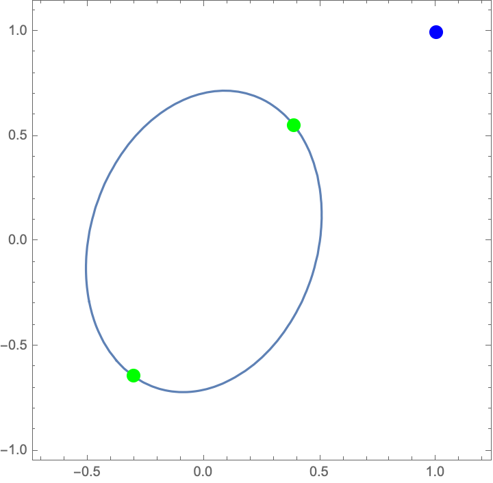
Figure 1. The ellipse $4x_{1}^{2}+2x_{2}^{2}-x_{1}x_{2}=1$ along with the critical points (green) of the Euclidean distance problem from the point $(1,1)$ (blue).

By B we know the number of complex critical points to this optimization problem will be ${\mathrm{MV}}(P_{1},P_{2},P_{3})$ where $P_{1}=\operatorname{conv}\{(1,0,0),(1,0,1),(0,1,1)\}$, $P_{2}=\operatorname{conv}\{(0,1,0),(1,0,1),(0,1,1)\}$ and $P_{3}=\operatorname{conv}\{(2,0,0),(0,2,0),(1,1,0),(0,0,0)\}$.

Now we consider the projective closure of our variety which is defined by $\overline{X}=\mathcal{V}(4x_{1}^{2}+2x_{2}^{2}-x_{1}x_{2}-x_{0}^{2})\subset\mathbb{P}^{2}$. The conormal variety of $\overline{X},\mathcal{N}_{\overline{X}}\subset\mathbb{P}^{2}\times(\mathbb{P}^{2})^{*}$ is defined as the zero set of the polynomials:

$$g_{1} =x_{1}y_{1}-4x_{2}y_{1}+8x_{1}y_{2}-x_{2}y_{2}$$

$$g_{2} =31y_{0}^{2}-8y_{1}^{2}-4y_{1}y_{2}-16y_{2}^{2}$$

$$g_{3} =31x_{2}y_{0}+2x_{0}y_{1}+16x_{0}y_{2}$$

$$g_{4} =31x_{1}y_{0}+8x_{0}y_{1}+2x_{0}y_{2}$$

$$g_{5} =x_{0}y_{0}+4x_{2}y_{1}-8x_{1}y_{2}+2x_{2}y_{2}$$

$$g_{6} =x_{0}^{2}-4x_{1}^{2}+x_{1}x_{2}-2x_{2}^{2}.$$

The $i$th polar degree $\delta_{i}(\overline{X})$ is given by the number of intersection points of $\mathcal{N}_{\overline{X}}\cap(L_{1}\times L_{2})$ where $L_{1}$ is a generic linear space of dimension $n+1-i$ and $L_{2}$ is a generic linear space of dimension $i$. In this case we have $\delta_{0}(\overline{X})=2$ and $\delta_{1}(\overline{X})=2$ and we see that the ED degree of $4x_{1}^{2}+2x_{2}^{2}-x_{1}x_{2}-1$ equals the sum of the polar degrees of its projective closure as expected.

Finally, we conclude this section by making a final connection to sectional degrees as recently studied in [MRWW23]. Given an affine variety $X\subset\mathbb{C}^{n}$, we define the $i$th sectional degree of $X$, $s_{i}(X)$ as the algebraic degree of the optimization problem

(SO) $$\min_{x\in\mathbb{R}^{n}}\ \langle u,x\rangle\quad\text{subject to}\quad x\in X\cap H_{1}\cap H_{2}\cap\cdots\cap H_{i}$$

where $u\in\mathbb{R}^{n}$ is a generic linear function and $H_{1},\ldots,H_{i}$ are generic affine linear hyperplanes. As an immediate consequence of B we have a convex algebraic interpretation of $s_{i}(X)$.

Corollary 4.7.

Let $X\subset\mathbb{C}^{n}$ be an affine variety defined by generic polynomials $(f_{1},\ldots,f_{m})$ with strongly admissible support. Let $\mathbf{L}_{\mathrm{F}}=(\ell_{1},\ldots,\ell_{n},f_{1},\ldots,f_{m})$ be the Lagrange system of $\mathbf{F}=(\langle u,x\rangle,f_{1},\ldots,f_{m})$ corresponding to the sectional optimization problem (SO). Then

$${\mathrm{MV}}({\mathrm{Newt}}(\ell_{1}),\ldots,{\mathrm{Newt}}(\ell_{n}),{\mathrm{Newt}}(f_{1}),\ldots,{\mathrm{Newt}}(f_{m}))=s_{i}(X)$$

where $s_{i}(X)$ is the $i$th sectional degree of $X$.

Furthermore, by [MRWW23, Corollary 6.8] we have that if $X\subset\mathbb{C}^{n}$ is an affine variety with projective closure $\overline{X}\subset\mathbb{P}^{n}$ such that $H_{\infty}$ is not contained in the dual of $\overline{X}$, then $s_{i}(X)=\delta_{i}(\overline{X})$ for all $0\leq i\leq\dim(X)$. Therefore, as a corollary of this and 4.5 we get an equality of mixed volumes. Given a polynomial system $\mathbf{F}=(f_{1},\ldots,f_{m})$ we use the notation ${\mathrm{MV}}(F)={\mathrm{MV}}({\mathrm{Newt}}(f_{1}),\ldots,{\mathrm{Newt}}(f_{m}))$.

Corollary 4.8.

Let $X\subset\mathbb{C}^{n}$ be an affine variety defined by polynomials $(f_{1},\ldots,f_{m})$ with strongly admissible support. For generic $u\in\mathbb{R}^{n}$, let $\mathbf{L}_{\mathrm{F}}$ be the Lagrange system of $\mathbf{F}=(\lVert x-u\rVert_{2}^{2},f_{1}\ldots,f_{m})$ corresponding to the Euclidean distance optimization problem (ED) and $\mathbf{L}_{F_{i}}$ the Lagrange system of $\mathbf{F}_{i}=(\langle u,x\rangle,f_{1},\ldots,f_{m})$ corresponding to the $i$th sectional optimization problem (SO). Assume that $H_{\infty}$ is not contained in the dual variety of $\overline{X}$. Then

$${\mathrm{MV}}(\mathbf{L}_{\mathrm{F}}) =\sum_{i=0}^{n-1}{\mathrm{MV}}(\mathbf{L}_{i}).$$

Observe that by the results in [MRWW23], we can think of sectional degrees as the affine analogue of polar degrees. With this in mind and the aforementioned results, we have the following conjecture.

Conjecture 4.9.

Let $X\subseteq\mathbb{C}^{n}$ be an irreducible, affine variety and $\overline{X}\subset\mathbb{P}^{n}$ its projective closure. If $\overline{X}$ intersects $Q_{\infty}$ transversely then the ED degree of $X$ is equal to $s_{0}(X)+\ldots+s_{n-1}(X)$.

To provide one piece of evidence for 4.9 we give an example where 4.9 is true but Theorem 4.4 gives a strict upped bound on the ED degree.

Example 4.10.

Consider the affine variety $X=\mathcal{V}(x_{1}^{2}-x_{2})\subset\mathbb{R}^{2}$. We can directly compute the ED degree of $X$ to be three. In this case, $X$ has two sectional degrees: $s_{0}(X)=1$ and $s_{1}(X)=2$. It is then clear that 4.9 holds in this case.

Conversely, we can consider the polar degrees of $\overline{X}=\mathcal{V}(x_{1}^{2}-x_{2}x_{0})$. Here, the conormal variety of $\overline{X}$ is defined as the common zero set of:

$$g_{1} =x_{2}y_{2}-x_{0}y_{0}$$

$$g_{2} =y_{1}^{2}-4y_{2}y_{0}$$

$$g_{3} =x_{0}y_{1}+2x_{1}y_{2}$$

$$g_{4} =x_{2}y_{1}+2x_{1}y_{0}$$

$$g_{5} =x_{1}y_{1}+2x_{0}y_{0}$$

$$g_{6} =x_{1}^{2}-x_{2}x_{0}.$$

With this, one can directly compute that $\delta_{0}(\overline{X})=2$ and $\delta_{1}(\overline{X})=2$. This provides an example where the sum of the polar degrees of $\overline{X}$ is a strict upper bound on the ED degree of $X$ but the sum of the sectional degrees is exact.

5. Homogeneous equations for critical points

In this section we define homogeneous critical point equations for the optimization problem (POP). We give two different sets of critical point equations for $\eqref{POP}$. On the one hand, in [NR09b] critical points are characterised as an intersection of the vanishing locus of homogeneous equations $\{\widetilde{f}_{1}=\cdots=\widetilde{f}_{m}=0\}$ with a projective determinantal variety $W$. We generalize this approach by replacing projective space with an appropriate toric variety $X$. On the other hand we homogenise the Lagrange equations $\mathbf{L}_{\mathrm{F}}=(f_{1},\ldots,f_{m},\ell_{1},\ldots,\ell_{n})$ in the Cox ring of a toric variety, $\mathbb{P}(\mathcal{E})$, which we introduce now. We show both approaches define the desired critical point equations in Lemma 5.8 with (5.2) concerning the former approach and (5.3) the latter.

5.1. Toric projective bundles

We now describe the toric structure on the projectivisation of a direct sum of line bundles on toric varieties. Let $X$ be a complete toric variety given by a fan $\Sigma$ and let $\mathcal{E}=\mathcal{L}_{0}\oplus\ldots\oplus\mathcal{L}_{m}$ be a fully decomposible vector bundle on $X$. In this subsection we will describe the fan of the total space of the projectivisation $\mathbb{P}(\mathcal{E})$. For a more general study of bundlea with toric variety fiber see [HKM23]. We will start with the a lemma:

Lemma 5.1.

Let $X$ be a toric variety and let $\mathcal{E}=\mathcal{L}_{0}\oplus\ldots\oplus\mathcal{L}_{m}$ be a vector bundle which is a direct sum of line bundles. The total spaces of $\mathcal{E}$ and $\mathbb{P}(\mathcal{E})$ have the structure of fibered toric varieties.

Proof.

The result follows from the fact that for every line bundle $\mathcal{L}_{i}$, there exists torus invariant divisor $D_{i}$ such that $\mathcal{L}_{i}=\mathcal{O}(D_{i})$. Therefore, each line bundle $\mathcal{L}_{i}$ on $X$ could be equipped with an equivariant structure, i.e. the action of $T$ on the total space of $\mathcal{L}_{i}$, which makes the projection map equivariant.

Now, fixing an equivariant structure on each of line bundles $\mathcal{L}_{i}$, we obtain a $T$-action on the total space of $\mathcal{E}$. Finally we extend $T$-action on $\mathcal{E}$ to the action of $T\times(\mathbb{C}^{*})^{m+1}$ by making the second component act fiberwise in a natural way. Clearly, this action is faithful and has open-dense orbit in the total space of $\mathcal{E}$.

Moreover, the action of $T\times(\mathbb{C}^{*})^{m+1}$ on $\mathcal{E}$ induces faithful action descends to an action on $\mathbb{P}(\mathcal{E})$. The latter action has a one dimensional kernel given by the diagonal subtorus in $(\mathbb{C}^{*})^{m+1}$. Hence $\mathbb{P}(\mathcal{E})$ has a structure of toric variety with respect to the factor torus

$$T\times\left((\mathbb{C}^{*})^{m+1}/\mathbb{C}^{*}\cdot(1,\ldots,1)\right).\qed$$

Remark 5.2.

Note that the divisor $D_{i}$ is defined up to addition of the principal divisor $div(u)$ of character $u\in\mathbb{Z}^{n}$ or equivalently, any two equivariant structures on $\mathcal{L}_{i}$ differ by the action of the character of $T$. However, the toric variety structures defined by different choices of $D_{i}$ are isomorphic (as toric varieties).

From now on assume that we fixed some $T$-invariant divisors $D_{i}$ such that $\mathcal{L}_{i}=\mathcal{O}(D_{i})$ for $i=0,\ldots,m$. Each such divisor defines a conewise-linear function

$$\psi_{i}\colon\mathbb{R}^{n}=|\Sigma|\to\mathbb{R}.$$

Let $\Psi=(\psi_{0},\ldots,\psi_{m})\colon|\Sigma|\to\mathbb{R}^{m+1}$ be the corresponding piecewise linear map.

Let us denote by $\widetilde{\Sigma}\subset\mathbb{R}^{n}\times\mathbb{R}^{m+1}$ a fan obtained as the graph of the function $\Psi$. That is, $\widetilde{\Sigma}$ consists of cones $\widetilde{\sigma}$ where

$$\widetilde{\sigma}=\{(y,\Psi(y))\,|\,y\in\sigma\},\text{ for }\sigma\in\Sigma.$$

Further, let $\mathbb{R}^{n}_{\geq 0}$ be the standard positive orthant in $\mathbb{R}^{m+1}$ considered as a fan in $\mathbb{R}^{n}\times\mathbb{R}^{m+1}$. Then the fan defining the total space of $\mathcal{E}$ consists of cones

$$\widetilde{\sigma}+\tau\text{ for }\sigma\in\Sigma,\tau\in\mathbb{R}^{n}_{\geq 0}.$$

Similarly, the fan $F$ defining the the total space of $\mathcal{E}$ with the zero section removed is given by

$$\widetilde{\sigma}+\tau\text{ for }\sigma\in\Sigma,\tau\in\partial\mathbb{R}^{n}_{\geq 0},$$

where $\partial\mathbb{R}^{n}_{\geq 0}$ is the relative boundary of the positive orthant in $\mathbb{R}^{m+1}$.

Finally, let $S_{0}\subset\mathcal{E}$ be the image of the zero section of $\mathcal{E}$. Clearly $S_{0}$ is a torus invariant subset of $\mathcal{E}$ and thus the natural projection of $\mathcal{E}\setminus S_{0}\to\mathbb{P}(\mathcal{E})$ is a toric morphism. Therefore the fan of the projectivisation $\mathbb{P}(\mathcal{E})$ is given by the projection of $\pi(F)$ where $\pi$ is the natural projection

$$\pi\colon\mathbb{R}^{n}\times\mathbb{R}^{m+1}\to\mathbb{R}^{n}\times\left(\mathbb{R}^{m+1}/\mathbb{R}\cdot(1,\ldots,1)\right).$$

Now let $S$ be the Cox ring of $X$, and let $S_{\mathcal{E}}$ be the Cox ring of $\mathbb{P}(\mathcal{E})$. By the above discussion, each ray of $\widetilde{\Sigma}$ is either of the form $\widetilde{\rho}$, where $\rho$ is a ray of $\Sigma$, or of the form $\{0\}\times e_{i}$, $i=1,\dots,m+1$. This splits the generators of $S_{\mathcal{E}}$ over $\mathbb{C}$ into two groups. The first group of generators $x_{\widetilde{\rho}}$ is bijective to the generators $x_{\rho}$ of $S$. We denote members of the second group by $\lambda_{i}=x_{\{0\}\times e_{i+1}}$ and obtain the following proposition.

Proposition 5.3.

The Cox ring of $S_{\mathcal{E}}$ is isomorphic to the free $S$-algebra $S[\lambda_{0},\dots,\lambda_{m}]$.

Remark 5.4.

In the following we are often in the situation that $f$ is a global section of a torus invariant line bundle $\mathcal{O}_{X}(D)$ on $X$. Now $\widetilde{f}$ denotes an element of $S\subseteq S_{\mathcal{E}}$. At the same time $f$ can be seen as a section of the bundle $\pi^{*}\mathcal{O}_{X}(D)$ on $\mathbb{P}(\mathcal{E})$. When homogenising, this gives rise to another element $\widetilde{f}\in S_{\mathcal{E}}$. Direct computation shows that there is no need for disambiguation, since both expressions are equal.

5.2. Homogeneous equations for critical points

We start by fixing some notation and definitions: For the rest of this section let $\mathbf{F}=(f_{0},\ldots,f_{m})$ be a generic sparse system of polynomials in $\mathbb{C}[X_{1},\ldots,X_{n}]$ with admissible support $\mathcal{A}=(\mathcal{A}_{0},\ldots,\mathcal{A}_{m})$. Furthermore $X$ denotes a toric variety that is appropriate for $\mathcal{A}$, with fan $\Sigma$.

Remark 5.5.

Note that, since $\Sigma$ contains the positive orthant $\mathbb{R}_{\geq 0}^{n}$ as a cone, there is a distinct copy of the affine space $\mathbb{C}^{n}$ contained in $X$. For clarity, in this section, we denote the variables in the coordinate ring $\mathbb{C}[X_{1},\ldots,X_{n}]$ of $\mathbb{C}^{n}$ in capital letters, while the generators of the Cox ring $S$ of $X$ are in lower case. By slight abuse of notation, we will denote the element $x_{e_{j}}$ in $S$ by $x_{j}$ for each $j=1\dots,n$.

For every $i=0,\dots,m$ let $\mathcal{L}_{i}=\mathcal{O}(-D_{f_{i}})$ denote the dual line bundle associated to $D_{f_{i}}$. Here $D_{f_{i}}$ is the torus invariant Weyl divisor on $X$, corresponding to the Newton polytope ${\mathrm{Newt}}(f_{i})$:

(5.1) $$D_{f_{i}}=\sum_{\rho\in\Sigma(1)}a_{\rho,i}D_{\rho},\quad\text{where}\quad a_{\rho,i}=-\min\{\langle m,\rho\rangle\ :\ m\in{\mathrm{Newt}}(f_{i})\}.$$

We denote by $\mathcal{E}$ the vector bundle $\mathcal{E}=\mathcal{L}_{0}\oplus\cdots\oplus\mathcal{L}_{m}$ with projectivized total space

$$\mathbb{P}(\mathcal{E})=\{(x,[\lambda])\mid\ x\in X,\ [\lambda]\in\mathbb{P}\left(\mathcal{E}(x)\right)\}.$$

The rest of this section is devoted to giving two different, but related, systems of homogeneous critical point equations for (POP), one in the Cox ring $S$ of $X$, and one in the Cox ring $S_{\mathcal{E}}$ of $\mathbb{P}(\mathcal{E})$. On the one hand, critical points are characterised by the vanishing of the Lagrange system $\mathbf{L}_{\mathrm{F}}$. It describes the intersection of the incidence variety

$$Z^{\circ}:=\{(x,[\lambda])\in\mathbb{C}^{n}\times\mathbb{P}^{n}:\ \left(\nabla f_{0}\mid\dots\mid\nabla f_{m}\right)\lambda=\underline{0}\}$$

with the vanishing locus of $f_{1},\dots,f_{m}$. On the other hand, critical points are characterized by the Jacobian $\left(\nabla f_{0}\mid\dots\mid\nabla f_{m}\right)$ dropping rank. They form the intersection $V^{\circ}\cap W^{\circ}$, where $V^{\circ}\coloneqq\mathcal{V}\left(f_{1},\dots,f_{m}\right)\subseteq\mathbb{C}^{n}$, and $W^{\circ}$ is the determinantal variety

$$W^{\circ}:=\{x\in\mathbb{C}^{n}\ :\ \operatorname{rank}\left(\nabla f_{0}\mid\dots\mid\nabla f_{m}\right)\leq m\}.$$

We proceed by giving homogeneous equations for $V^{\circ},W^{\circ}$ and $Z^{\circ}$ in $S$ and $S_{\mathcal{E}}$ respectively. Every polynomial $f_{i}$ is a global section of the line bundle $\mathcal{O}_{X}(D_{f_{i}})$, and its homogeneous form can be written as

$$\widetilde{f_{i}}=\sum_{m\in{\mathrm{Newt}}(f_{i})\cap\mathbb{Z}^{n}}c_{m,i}\prod_{\rho\in\Sigma(1)}x_{\rho}^{\langle m,\rho\rangle+a_{\rho,i}}.$$

Here we homogenize $f_{i}$ as in (2.1) in Section 2.2. In particular, $\widetilde{f}_{i}$ is defined by our choice of line bundle $\mathcal{O}_{X}(D_{f_{i}})$.

We denote by $V$ the closure of $V^{\circ}=\mathcal{V}\left(f_{1},\dots,f_{m}\right)$ in $X$. Observe that by genericity of $\mathbf{F}$, $V$ is equal to the vanishing locus of the homogeneous equations $V=\mathcal{V}\left(\widetilde{f}_{1},\dots\widetilde{f}_{m}\right).$

From now on $M$ denotes a homogeneous version of the Jacobian matrix:

$$M=\left(\widetilde{\nabla}\widetilde{f}_{0}\mid\dots\mid\widetilde{\nabla}\widetilde{f}_{m}\right).$$

Here $\widetilde{\nabla}$ denotes the vector $(\frac{\partial}{\partial x_{1}},\dots,\frac{\partial}{\partial x_{n}})^{T},$ so $M$ has columns $\left(\frac{\partial}{\partial x_{1}}\widetilde{f}_{i},\dots,\frac{\partial}{\partial x_{n}}\widetilde{f}_{i}\right)^{T}$. We define

$$W\coloneqq\{x\in X\ :\ \operatorname{rank}M(x)\leq m\}$$

to be the vanishing locus of the maximal minors of $M$, and furthermore we let

$$Z\coloneqq\{(x,[\lambda])\in\mathbb{P}(\mathcal{E})\ :\ M(x)\lambda=0\}$$

be the associated incidence variety, contained in the projectivized total space $\mathbb{P}(\mathcal{E})$.

The rest of this Section is devoted to proving Lemma 5.8. It shows that the homogeneous critical point equations agree with the affine ones when restricted to affine space $\mathbb{C}^{n}$.

We need an observation about differentiating homogeneous polynomials. Let $D$ be a torus invariant Weyl divisor on $X$ (or on $\mathbb{P}(\mathcal{E})$), and $f$ a global section of $\mathcal{O}_{X}(D)$. Observe that for $j=1,\dots,n$ the Newton polytope of the differential $X_{j}\frac{\partial}{\partial X_{j}}f$ is contained in the rational polytope $e_{j}+\partial_{j}{\mathrm{Newt}}(f)$, and in particular $\frac{\partial}{\partial X_{j}}f$ is a global section of the sheaf $\frac{1}{X_{j}}\mathcal{O}_{X}(D-D_{e_{j}})$ (or of the sheaf $\frac{1}{X_{j}}\mathcal{O}_{\mathbb{P}(\mathcal{E})}(D-D_{\widetilde{e}_{j}})$). Direct computation shows the following proposition.

Proposition 5.6.

Homogenisation and differentiation commute: $\widetilde{\frac{\partial}{\partial X_{j}}f}=\frac{\partial}{\partial x_{j}}\widetilde{f}$.

We denote by $\widetilde{\Phi}_{F}$ the homogenization of the Lagrangian $\Phi$, living in the Cox ring $S_{\mathcal{E}}$. This makes sense since $\mathbb{P}(\mathcal{E})$ is a global section of the sheaf $\mathcal{O}_{\mathbb{P}(\mathcal{E})}(D_{\Phi_{F}})$, associated to the Cayley polytope ${\mathrm{Newt}}(\Phi_{F})={\mathrm{Cay}}({\mathrm{Newt}}(f_{0}),\dots,{\mathrm{Newt}}(f_{m}))$. By the above Proposition, each of the defining equations

$$0=\left(M(x)\lambda\right)_{j}=\lambda_{0}\frac{\partial}{\partial x_{j}}\widetilde{f}_{0}+\cdots+\lambda_{m}\frac{\partial}{\partial x_{j}}\widetilde{f}_{m}=\frac{\partial}{\partial x_{j}}\widetilde{\Phi}_{F}(\lambda,x)$$

of $Z$ is equal to the homogenisation $\widetilde{\ell_{j}}$ of $\ell_{j}=\widetilde{\frac{\partial}{\partial X_{j}}\Phi_{F}}(\lambda,x)$. Here $\widetilde{\ell_{j}}$ is identified with a global section of the sheaf $\mathcal{O}_{\mathbb{P}(\mathcal{E})}(D_{\Phi_{F}}-D_{\widetilde{e}_{j}})$.

We denote by $\widetilde{\mathbf{L}}_{F}=(\widetilde{f}_{1},\ldots,\widetilde{f}_{m},\widetilde{\ell}_{1},\ldots,\widetilde{\ell}_{n})$ the homogenized Lagrange system. On the one hand, we observed above that $Z$ is equal to the vanishing locus of $\widetilde{\ell}_{1},\ldots,\widetilde{\ell}_{n}$. On the other hand, the vanishing locus of $(\widetilde{f}_{1},\ldots,\widetilde{f}_{m})$ in $\mathbb{P}(\mathcal{E})$ is the preimage $\pi^{-1}(V)$ of the vanishing locus $V$ in $X$. We obtain the following Proposition.

Proposition 5.7.

The vanishing locus of  $\widetilde{\mathbf{L}}_{F}$ in $\mathbb{P}(\mathcal{E})$ is the intersection $Z\cap\pi^{-1}(V)$.

The following lemma shows that the homogeneous critical point equations introduced in this chapter restrict, on $\mathbb{C}^{n}$, to the expected affine critical point equations.

Lemma 5.8.

The following three equalities hold:

(5.2) $$V\cap\mathbb{C}^{n}=V^{\circ},\quad\ W\cap\mathbb{C}^{n}=W^{\circ}$$

(5.3) $$Z\cap\left(\mathbb{C}^{n}\times\mathbb{P}^{n}\right)=Z^{\circ}$$

where the intersection in (5.2) is on $X$ and the intersection in (5.3) is on $\mathbb{P}(\mathcal{E})$.

Proof.

The first of the equalities is clear, by the definition of $V$ as the closure of $V^{\circ}$. To see the second equality, we prove that the entries of $M$ are homogenizations of the entries of the Jacobian $\left(\nabla{f}_{0},\dots,\nabla{f}_{m}\right)$. This is a direct consequence of Proposition 5.6, since for every $i=0,\dots,m$ and $j=1,\dots,n$ it holds $\widetilde{\frac{\partial}{\partial X_{j}}f_{i}}=\frac{\partial}{\partial x_{j}}\widetilde{f}_{i}$. The third equality is analogous, since homogenising the defining equations ${\ell}_{1},\dots\ell_{n}$ of $Z^{\circ}$ yields the defining equations $\widetilde{\ell}_{1},\dots\widetilde{\ell}_{n}$ of $Z$. ∎

We close this section with the following generalization of the Euler equation.

Proposition 5.9.

Let $D=\sum_{\rho\in\Sigma(1)}a_{\rho}D_{\rho}$ be a torus invariant Weyl divisor, $f$ a global section of $\mathcal{O}_{X}(D)$ and $\tau\in\Sigma(1)$ a ray. Then the generalized Euler equation

(5.4) $$-x_{\tau}\frac{\partial}{\partial x_{\tau}}\widetilde{f}+\tau_{1}x_{1}\frac{\partial}{\partial x_{1}}\widetilde{f}+\cdots+\tau_{n}x_{n}\frac{\partial}{\partial x_{n}}\widetilde{f}=-a_{\tau}\widetilde{f}$$

holds for the homogenization $\widetilde{f}\in S$ of $f$.

Proof.

Equation (2.1) reads $\widetilde{f}=\sum_{m\in\mathbb{Z}^{n}}c_{m}\prod_{\rho\in\Sigma(1)}x_{\rho}^{\langle m,\rho\rangle+a_{\rho}}$ and we have

$$-x_{\tau}\frac{\partial}{\partial x_{\tau}}\widetilde{f}+\tau_{1}x_{1}\frac{\partial}{\partial x_{1}}\widetilde{f}+\cdots+\tau_{n}x_{n}\frac{\partial}{\partial x_{n}}\widetilde{f}$$

$$= \sum_{m\in\mathbb{Z}^{n}}c_{m}\left(-x_{\tau}\frac{\partial}{\partial x_{\tau}}+\tau_{1}x_{1}\frac{\partial}{\partial x_{1}}+\cdots+x_{n}\frac{\partial}{\partial x_{n}}\right)\prod_{\rho\in\Sigma(1)}x_{\rho}^{\langle m,\rho\rangle+a_{\rho}}$$

$$= \sum_{m\in\mathbb{Z}^{n}}c_{m}(-\langle m,\tau\rangle-a_{\tau}+m_{1}+a_{e_{1}}+\cdots+m_{n}+a_{e_{n}})\prod_{\rho\in\Sigma(1)}x_{\rho}^{\langle m,\rho\rangle+a_{\rho}}$$

$$= \sum_{m\in\mathbb{Z}^{n}}c_{m}(-a_{\tau})\prod_{\rho\in\Sigma(1)}x_{\rho}^{\langle m,\rho\rangle+a_{\rho}}=-a_{\tau}\widetilde{f}.\qed$$

6. Computing the number of critical points

In Section 5 we characterized critical points of (POP) in two ways. On the one hand, as an intersection $V\cap W$ in $X$ as in (5.2) of Lemma 5.8,

and on the other hand by means of homogenized Lagrange equations $\widetilde{\mathbf{L}}_{F}$ in the Cox ring of $\mathbb{P}(\mathcal{E})$ as in (5.3) of Lemma 5.8. In this section we show that all intersections are transversal and happen in $\mathbb{C}^{n}$. This characterises the number of critical points as products of cohomology classes? In the case of Theorem A this product is a mixed volume. The proof of Theorem C rests on a characterization of $[W]$ as a Porteus’ class.

6.1. Preliminary results

We start by proving some technical statements that are needed for the the desired transversality results. For the rest of the section we again fix the assumptions from 5.2, and furthermore assume that $V$ does not intersect the singular locus of $X$. It follows from Bertini’s Theorem, that $V$ is smooth.

For the next proposition we need the following notion. Similar to the projection $\mathbb{C}^{n+1}\setminus\{0\}\to\mathbb{P}^{n}$, there exists the open subset $U_{\Sigma}\subseteq\mathbb{C}^{\Sigma(1)}$ with a projection $\tau:U_{\Sigma}\to X$. For a subvariety $V$ of $X$, we define the cone $C(Y)$ over $Y$ to be the closure of the preimage $\tau^{-1}(Y)$ in $\mathbb{C}^{\Sigma(1)}$. The intersection $C(Y)\cap U_{\Sigma}$ forms a torus principle bundle over $Y$. In particular, $C(Y)\cap U_{\Sigma}$ is smooth if $Y$ is smooth.

Proposition 6.1.

The matrices $M=\left(\widetilde{\nabla}\widetilde{f}_{0},\dots,\widetilde{\nabla}\widetilde{f}_{m}\right)$ and $\left(\widetilde{\nabla}\widetilde{f}_{1},\dots,\widetilde{\nabla}\widetilde{f}_{m}\right)$ have full ranks $m+1$ and $m$ everywhere on $\mathcal{V}\left(\widetilde{f}_{0},\dots\widetilde{f}_{m}\right)$ and $\mathcal{V}\left(\widetilde{f}_{1},\dots\widetilde{f}_{m}\right)$ respectively.

Proof.

The proof for the second matrix is analogous, so we only do the proof for

$$M=\left(\widetilde{\nabla}\widetilde{f}_{0},\dots,\widetilde{\nabla}\widetilde{f}_{m}\right).$$

Let $x\in\mathcal{V}\left(\widetilde{f}_{0},\dots\widetilde{f}_{m}\right)$ be arbitrary and $\sigma\in\Sigma$ the unique cone such that $x$ is contained in the torus orbit $O(\sigma)$. Let $\widetilde{M}$ denote the matrix with rows

(6.1) $$\left(\frac{\partial}{\partial x_{\rho}}\widetilde{f}_{0},\dots,\frac{\partial}{\partial x_{\rho}}\widetilde{f}_{m}\right)$$

for each ray $\rho$ in $\Sigma(1)$. The left kernel of $\widetilde{M}$ is the tangent space of the cone $C\left(\mathcal{V}\left(\widetilde{f}_{0},\dots,\widetilde{f}_{m}\right)\right)$ in $\mathbb{C}^{\Sigma(1)}$. The Jacobian $\widetilde{M}_{\sigma}$, of the cone over the variety $O(\sigma)\cap\mathcal{V}\left(\widetilde{f}_{0},\dots,\widetilde{f}_{m}\right)$ is a submatrix of $\widetilde{M}$. Its rows correspond to those rays $\rho$ that are not contained in $\sigma$. By Bertini’s Theorem $\mathcal{V}\left(\widetilde{f}_{0},\dots,\widetilde{f}_{m}\right)$ is a smooth variety. Further the intersection $O(\sigma)\cap\mathcal{V}\left(\widetilde{f}_{0},\dots,\widetilde{f}_{m}\right)$ is transversal by [Kho78], so $\widetilde{M}_{\sigma}$ is of full rank $m+1$ at $x$. We now finish the proof by showing that the row span of $\widetilde{M}_{\sigma}$ is contained in the row span of $M$. Let $\rho$ be any ray that is not contained in $\sigma$. To show that the corresponding row (6.1) of $\widetilde{M}_{\sigma}$ is contained in the row span of $M$, we apply Proposition 5.9 to all functions $\widetilde{f}_{0},\dots,\widetilde{f}_{m}$. The right side of equation $\eqref{eq:Euler formula}$ vanishes, and we obtain

$$\begin{pmatrix}\rho_{1}x_{1}\\ \vdots\\ \rho_{n}x_{n}\end{pmatrix}^{T}M=x_{\rho}\begin{pmatrix}\frac{\partial}{\partial x_{\rho}}\widetilde{f}_{0}\\ \vdots\\ \frac{\partial}{\partial x_{\rho}}\widetilde{f}_{m}\end{pmatrix}^{T}.\qed$$

Proposition 6.2.

The gradient $\widetilde{\nabla}\widetilde{f}_{0}$ does not vanish uniformly on any torus orbit.

Proof.

Towards a contradiction we assume that there exists a cone $\sigma\in\Sigma$ such that for every $j=1,\dots,n$ the polynomial $\frac{\partial}{\partial x_{j}}\widetilde{f}_{0}$ vanishes on the associated torus orbit $O(\sigma)$ of $X$. We denote by $\left.\frac{\partial}{\partial x_{j}}\widetilde{f}_{0}\right|_{O(\sigma)}$ the restriction of $\frac{\partial}{\partial x_{j}}\widetilde{f}_{0}$ to the cone over $O(\sigma)$. It is obtained by substituting all variables $x_{\rho}$ with zero, where $\rho$ is contained in $\sigma$.

Now consider the face ${\mathrm{Newt}}(f_{0})^{\sigma}$ of ${\mathrm{Newt}}(f_{0})$ exposed by $\sigma$. For every lattice point $m$ of ${\mathrm{Newt}}(f_{0})^{\sigma}$ the monomial

$$\frac{\partial}{\partial x_{j}}\prod_{\rho\in\Sigma(1)}x_{\rho}^{\langle m,\rho\rangle+a_{\rho,0}},\quad a_{\rho,0}=-\min\{\langle m,\rho\rangle\ :\ m\in{\mathrm{Newt}}(f_{0})\}$$

of $\frac{\partial}{\partial x_{j}}\widetilde{f}_{0}$ only vanishes on $O(\sigma)$ if $m_{j}=0$. In particular, the face ${\mathrm{Newt}}(f_{0})^{\sigma}$ can only contain the single element $\underline{0}$. By assumption 3.2 on $X$, $\underline{0}$ is a smooth vertex of ${\mathrm{Newt}}(f_{0})$, and dual to the cone $\mathbb{R}_{\geq 0}^{n}$. Since $\sigma$ reveals the vertex $\underline{0}$, it has to intersect the interior of the positive orthant $\mathbb{R}_{\geq 0}^{n}$ and in fact both cones are equal. This leaves us with the case where the torus orbit is $\{\underline{0}\}$. But the gradient of $f_{0}$ does not vanish uniformly at $\underline{0}$. ∎

Proposition 6.3.

The variety $V\cap W$ is of dimension $0$.

Proof.

Towards a contradiction we assume that there exists a torus orbit $O(\sigma)$, and a curve $C$ such that $C$ is contained in the intersection $W\cap V\cap O(\sigma)$. We denote by $\left.\widetilde{f}_{0}\right|_{O(\sigma)}$ the restriction of $\widetilde{f}_{0}$ to $O(\sigma)$. It is obtained by substituting all variables $x_{\rho}$ with zero, where $\rho$ is contained in $\sigma$. We now distinguish two cases: either $\left.\widetilde{f}_{0}\right|_{O(\sigma)}$ vanishes somewhere on $O(\sigma)$, or it is a scalar multiple of a monomial. In the first case $\left.\widetilde{f}_{0}\right|_{O(\sigma)}$ vanishes on $C$ by genericity. In particular, the matrix $M$ drops rank somewhere on the vanishing locus $\mathcal{V}\left(\widetilde{f}_{0},\dots\widetilde{f}_{m}\right)$, contradicting Proposition 6.1.

In the second case we derive a contradiction from Proposition 6.1 by showing that the matrix $\left(\widetilde{\nabla}\widetilde{f}_{1},\dots,\widetilde{\nabla}\widetilde{f}_{m}\right)$ drops rank somewhere on $C$. Suppose $\left.\widetilde{f}_{0}\right|_{O(\sigma)}$ is a monomial. Then each restriction $\left.\frac{\partial}{\partial x_{j}}\widetilde{f}_{0}\right|_{O(\sigma)}$ is either a monomial or zero, and by Proposition 6.2 there is an index $l=1,\dots,n$ such that $\left.\frac{\partial}{\partial x_{l}}\widetilde{f}_{0}\right|_{O(\sigma)}$ is not zero. Without loss of generality we assume $l$ to be $1$. Consider the following matrix, $M^{*}$, obtained by subtracting for each $j=2,\dots,n$ from the $j-$th row of $M$ the multiple

$$\frac{\frac{\partial}{\partial x_{j}}\widetilde{f}_{0}}{\frac{\partial}{\partial x_{1}}\widetilde{f}_{0}}\left(\frac{\partial}{\partial x_{1}}\widetilde{f}_{0},\dots,\frac{\partial}{\partial x_{1}}\widetilde{f}_{m}\right)$$

of the first row, eliminating the first entry in the process:

$$M^{*}=\begin{bmatrix}\frac{\partial}{\partial x_{1}}\widetilde{f}_{0}&\frac{\partial}{\partial x_{1}}\widetilde{f}_{1}\dots\frac{\partial}{\partial x_{1}}\widetilde{f}_{m}\\ \begin{matrix}0\\ \vdots\\ 0\end{matrix}&\Huge{A}\end{bmatrix}.$$

Since $M$ drops rank everywhere on $C$ and $\frac{\partial}{\partial x_{1}}\widetilde{f}_{0}$ is not identically zero, $A$ also drops rank on $C$. Let $\mu=\left(\mu_{1},\dots,\mu_{n}\right)^{T}$ be a vector of rational functions on $O(\sigma)$ satisfying

$$A\mu=0$$

everywhere on $C$. Since the expression $\mu_{1}\frac{\partial}{\partial x_{1}}\widetilde{f}_{1}+\dots+\mu_{n}\frac{\partial}{\partial x_{n}}\widetilde{f}_{1}$, is not a monomial on $O(\sigma)$, it vanishes at some point $x$ in $C$ by genericity. This shows that $\mu(x)$ is in the right kernel of $\left(\widetilde{\nabla}\widetilde{f}_{1}(x),\dots,\widetilde{\nabla}\widetilde{f}_{m}(x)\right)$, finishing the proof. ∎

Lemma 6.4.

The intersection $Z\cap\mathcal{V}(\widetilde{f}_{1},\dots,\widetilde{f}_{m})$ is transversal and contained in the big torus $(\mathbb{C}^{*})^{n+m}$ in the toric variety $\mathbb{P}(\mathcal{E})$.

Proof.

The image of $Z\cap\mathcal{V}(\widetilde{f}_{1},\dots,\widetilde{f}_{m})$ under the natural projection $\pi:\mathbb{P}(\mathcal{E})\longrightarrow X$ is $W\cap\mathcal{V}(\widetilde{f}_{1},\dots,\widetilde{f}_{m})$, which by Proposition 6.3 is finite. In fact, we prove below that $\pi$ bijectively identifies both sets. In particular, the $n$ defining equations of $Z$, given by $M(x)\lambda=0$, form a complete intersection when restricted to $\mathcal{V}(\widetilde{f}_{1},\dots,\widetilde{f}_{m})$.

To inductively apply Bertini we now show that, for varying coefficients of $f_{0}$, $Z\cap\mathcal{V}(\widetilde{f}_{1},\dots,\widetilde{f}_{m})$ defines a basepoint free family of varieties on the vanishing locus $\mathcal{V}(\widetilde{f}_{1},\dots,\widetilde{f}_{m})$ in $\mathbb{P}(\mathcal{E})$. To do this, we fix any element $x$ of $V$ and show that $Z$ does not have a fixed point in the fiber $\pi^{-1}(x)$. By Proposition 6.1 the last $m$ columns $\left(\widetilde{\nabla}\widetilde{f}_{1},\dots,\widetilde{\nabla}\widetilde{f}_{m}\right)$ of $M$ are linearly independent. In particular, varying the first column $\widetilde{\nabla}\widetilde{f}_{0}$ changes the unique solution $[\lambda]$ to $M(x)\lambda=0$. It now suffices to see that the gradient $\widetilde{\nabla}\widetilde{f}_{0}$ does not vanish uniformly at $x$, which by Proposition 6.2 is true for generic coefficients of $f_{0}$. To finally see that $Z\cap\mathcal{V}(\widetilde{f}_{1},\dots,\widetilde{f}_{m})$ is contained in the big torus orbit, we apply the same Bertini type argument to show transversality of the intersection $O\cap\mathcal{V}\left(\widetilde{f}_{1},\dots,\widetilde{f}_{m}\right)\cap Z$. Here $O$ denotes any torus orbit on $\mathbb{P}(\mathcal{E})$. For dimensional reasons only for the big torus this intersection can be non empty. ∎

6.2. The proof of A

The idea behind the proof of A is to study the system of homogenized Lagrange equations $\widetilde{\mathbf{L}}_{F}=(\widetilde{f}_{1},\ldots,\widetilde{f}_{m},\widetilde{\ell}_{1},\ldots,\widetilde{\ell}_{n})$. We will show that it comprises global sections of $\mathbb{Q}$-Cartier divisors, that intersect transversally and away from infinity. This expresses the number of solutions as a product of Chern classes, which is a mixed volume.

For the rest of this subsection we impose the assumptions of Theorem A. Let $\Sigma$ be the normal fan of the Minkowski sum of the polytopes ${\mathrm{Newt}}(f_{0}),\dots,{\mathrm{Newt}}(f_{n})$, and let $X$ be the associated normal toric variety. Then the assumptions from the beginning of Subsection 5.2 are fulfilled, since $X$ is appropriate for $\mathcal{A}$, and $V$ does not intersect the singular locus of $X$.

For each $j=1,\dots,n$, we defined the homogenisation $\widetilde{\ell}_{j}$ of $\ell_{j}$ as a section of the divisor $D_{\Phi_{F}}-D_{\widetilde{e}_{j}}$ on $\mathbb{P}(\mathcal{E})$. We first prove that this divisor is associated to the rational polytope $\partial_{j}{\mathrm{Newt}}(\Phi_{F})$.

Lemma 6.5.

For all $j=1,\dots,n$, the divisor $D_{\Phi_{F}}-D_{\widetilde{e}_{j}}$ on $\mathbb{P}(\mathcal{E})$ is rationally equivalent to the divisor associated to the rational polytope $\partial_{j}{\mathrm{Newt}}(\Phi_{F})$. In particular, the sheaf $\mathcal{O}_{\mathbb{P}(\mathcal{E})}(D_{\Phi_{F}}-D_{\widetilde{e}_{j}})$ is basepeoint free.

Proof.

We now prove that the divisor $D_{\Phi_{F}}-D_{\widetilde{e}_{j}}$ is associated to the polytope $e_{j}+\partial_{j}{\mathrm{Newt}}(\Phi_{F})$. Note that $e_{j}+\partial_{j}{\mathrm{Newt}}(\Phi_{F})$ is the intersection of ${\mathrm{Newt}}(\Phi_{F})$ with the affine halfspace $\{x_{j}\geq 1\}$. We have to prove that the support function of ${\mathrm{Newt}}(\Phi_{F})\cap{\{x_{j}\geq 1\}}$ takes the same value on all rays of $\Sigma_{\mathcal{E}}$, except for $\widetilde{e_{j}}$, where it differs by one. Let $v$ be any element of $\mathbb{R}^{n+m}$. The value

$$-\min\{\langle w,v\rangle\ :\ w\in{\mathrm{Newt}}(\Phi_{F})\}$$

of the support function of ${\mathrm{Newt}}(\Phi_{F})$ on $v$ can only differ if the face ${\mathrm{Newt}}(\Phi_{F})^{v}$ is contained in the facet

$${\mathrm{Newt}}(\Phi_{F})^{\widetilde{e}_{j}}={\mathrm{Newt}}(\Phi_{F})\cap{\{x_{j}=0\}}.$$

Since a face of the form ${\mathrm{Newt}}(\Phi_{F})^{\{0\}\times e_{i}}$ is always a facet, we may restrict to rays of the form $\widetilde{\rho}.$ Let now $\widetilde{\rho}$ be a ray such that ${\mathrm{Newt}}(\Phi_{F})^{\widetilde{\rho}}$ is contained in ${\mathrm{Newt}}(\Phi_{F})^{\widetilde{e}_{j}}$. By Proposition 6.6 below we have

$$\,{\mathrm{Cay}}\left({\mathrm{Newt}}(f_{0})^{\rho},\dots,{\mathrm{Newt}}(f_{m})^{\rho}\right)$$

$$= \,{\mathrm{Newt}}(\Phi_{F})^{\widetilde{\rho}}$$

$$\subseteq \,{\mathrm{Newt}}(\Phi_{F})^{\widetilde{e_{j}}}$$

$$= \,{\mathrm{Cay}}\left({\mathrm{Newt}}(f_{0})^{e_{j}},\dots,{\mathrm{Newt}}(f_{m})^{e_{j}}\right),$$

implying ${\mathrm{Newt}}(f_{i})^{\rho}\subseteq{\mathrm{Newt}}(f_{i})^{e_{j}}$ for all $i=0,\dots,m$. We obtain

$$\left(\sum_{i=0}^{n}{\mathrm{Newt}}(f_{i})\right)^{\rho}=\sum_{i=0}^{n}{\mathrm{Newt}}(f_{i})^{\rho}\subseteq\sum_{i=0}^{n}{\mathrm{Newt}}(f_{i})^{e_{j}}\left(\sum_{i=0}^{n}{\mathrm{Newt}}(f_{i})\right)^{e_{j}},$$

which is an inclusion of facets of the Minkowski sum $\sum_{i=0}^{m}{\mathrm{Newt}}(f_{i})$, showing the equality $\rho=e_{j}$. ∎

Proposition 6.6.

Let $\sigma$ be a cone in the normal fan $\Sigma(P_{1}+\cdots+P_{n})$. Then the face of ${\mathrm{Cay}}(P_{1},\dots,P_{n})$ exposed by $\widetilde{\sigma}$ is equal to the Cayley polytope of the faces $P_{1}^{\sigma},\dots,P_{n}^{\sigma}$:

(6.2) $${\mathrm{Cay}}(P_{1},\dots,P_{n})^{\widetilde{\sigma}}={\mathrm{Cay}}(P_{1}^{\sigma},\dots,P_{n}^{\sigma}).$$

Proof.

This can be done by direct computation. A different argument relies on Proposition A.4. For this, denote by $X_{\sigma}$ the closure of the torus orbit of $X_{\Sigma}$ corresponding to $\sigma\in\Sigma$. By Proposition A.4, the equation (6.2) is equivalent to the equality

$$\mathcal{O}_{\mathbb{P}(\mathcal{E})}(1)\big{|}_{X_{\Sigma}}=\mathcal{O}_{\mathbb{P}(\mathcal{E}|_{X_{\Sigma}})}(1).\qed$$

Before proving Theorem A we need to show a statement about the intersection of $\mathbb{Q}$-Cartier divisors.

Lemma 6.7 (Generic intersection of $\mathbb{Q}$-cartier divisors).

Let $X$ be a normal, proper variety of dimension $n$ with Weyl divisors $D_{1},\dots,D_{n}$, and let $k$ be an integer such that $\mathcal{O}(kD_{i})$ is a line-bundle for each $i=1,\dots,n$. Let $\widetilde{f_{i}}$ be a global section of $\mathcal{O}(D_{i})$ for $i=1,\dots,n$ such that $\mathcal{V}(\widetilde{f}_{1},\dots,\widetilde{f}_{n})$ is a zero dimensional smooth scheme contained in the smooth locus of $X$. Then

$$k^{n}\#\mathcal{V}(\widetilde{f}_{1},\dots,\widetilde{f}_{n})=c_{1}(\mathcal{O}(kD_{1}))\cdots c_{1}(\mathcal{O}(kD_{n})).$$

Proof.

The length of the zero dimensional scheme $\mathcal{V}(\widetilde{f}_{1}^{k},\dots,\widetilde{f}_{n}^{k})$ is equal to the product $c_{1}(\mathcal{O}(kD_{1}))\cdots c_{1}(\mathcal{O}(kD_{n}))$ of Chern classes. On the other hand, since $\widetilde{f}_{1},\dots,\widetilde{f}_{n}$ intersect transversally, each isolated point of $\mathcal{V}(\widetilde{f}_{1}^{k},\dots,\widetilde{f}_{n}^{k})$ is isomorphic to the scheme $\operatorname{Spec}\mathbb{C}[x_{1},\dots,x_{n}]/\langle x_{1}^{k},\dots,x_{n}^{k}\rangle$. In particular we have

$$k^{n}\operatorname{length}(\mathcal{V}(\widetilde{f}_{1},\dots,\widetilde{f}_{m}))=\operatorname{length}(\mathcal{V}(\widetilde{f}_{1}^{k},\dots,\widetilde{f}_{n}^{k})),$$

finishing the proof. ∎

Proof of Theorem A.

The vanishing locus of the homogenized system of Lagrange equations $\widetilde{\mathbf{L}}_{F}=(\widetilde{f}_{1},\ldots,\widetilde{f}_{m},\widetilde{\ell}_{1},\ldots,\widetilde{\ell}_{n})$ is the intersection of $Z$ with the vanishing locus of $\widetilde{f}_{1},\ldots,\widetilde{f}_{m}$ and by Lemma 6.4 this intersection is a smooth zero dimensional variety, contained in the big torus. By Lemma 5.8, the algebraic degree of sparse polynomial optimization is equal to its cardinality. According to Lemma 6.5, the system $\widetilde{\mathbf{L}}_{F}$ comprises global sections of $\mathbb{Q}$-Cartier divisors, associated to the respective, rational, polytopes ${\mathrm{Newt}}(f_{1}),\dots,{\mathrm{Newt}}(f_{m}),\partial_{1}{\mathrm{Newt}}(\Phi_{F}),\dots,\partial_{n}{\mathrm{Newt}}(\Phi_{F}).$ As a consequence of Lemma 6.7, and using multilinearity of the mixed volume, we can express the number of solutions to $\widetilde{\mathbf{L}}_{F}$ as the mixed volume (3.1) of these polytopes. ∎

6.3. The proof of Theorem C

In this section we study the intersection of the determinantal variety $W$ with the vanishing locus $V$ of $\widetilde{f}_{1},\ldots,\widetilde{f}_{m}$ in $X$. The proof of Theorem C rests on a proof of transversality, and a characterisation of the cohomology class $[W]$ as a Porteus’ class.

We start by recalling Porteous’ formula, also called the Giambelli–Thom–Porteous formula. For more details refer to [Ful98] and [EH16]. The following statement is a special case of Theorem 12.4 in [EH16].

Theorem 6.8.

(Porteus’ formula) Let $\varphi:\mathcal{E}\longrightarrow\mathcal{F}$ be a morphism of vector bundles of ranks $m+1\leq n$ on a smooth proper variety $X$ of dimension $n$. We denote by $W$ the (possibly non reduced) degeneracy locus of $\varphi$, supported on the set

$$|W|=\{x\in X\ :\ \varphi_{x}:\mathcal{E}(x)\longrightarrow\mathcal{F}(x)\textrm{ is not injective}\}.$$

If $W$ is pure of codimension $n-m$ then the cohomology class of $W$ is the $n-m$ graded part

$$\left[W\right]=\left(\operatorname{s}(\mathcal{E})\operatorname{c}(\mathcal{F})\right)_{n-m}$$

of the product of the total Segre class $\operatorname{s}(\mathcal{E})$ and the total Chern class $\operatorname{c}(\mathcal{F})$.

We need the following, modified version of Porteus’ formula which only requires $W$ to be pure dimensional after restricting to a subvariety $V$ of $X$.

Corollary 6.9.

Under the assumptions of Theorem 6.8, let $V$ be an irreducible closed subvariety of $X$ of codimension $k$, which intersects $W$ transversally and let the intersection $V\cap W$ be pure of codimension $n-m+k$. Then the cohomology class $\left[V\cap W\right]$ is given by

$$\left[V\cap W\right]=\left[V\right]\cdot\left(\operatorname{s}(\mathcal{E})\operatorname{c}(\mathcal{F})\right)_{n-m}.$$

Proof.

Note that $V\cap W$ is the degeneracy locus of the restriction $\left.\varphi\right|_{V}$. By applying Porteous formula to $\phi|_{V}\colon\mathcal{E}|_{V}\to\mathcal{F}|_{V}$ we get

$$[V\cap W]=\left(\operatorname{s}(\left.\mathcal{E}\right|_{V})\operatorname{c}(\left.\mathcal{F}\right|_{V})\right)_{n-m+k}.$$

Lastly we notice that $\left(\operatorname{s}(\left.\mathcal{E}\right|_{V})\operatorname{c}(\left.\mathcal{F}\right|_{V})\right)_{n-m+k}=\left[V\right]\cdot\left(\operatorname{s}(\mathcal{E})\operatorname{c}(\mathcal{F})\right)_{n-m}$ by naturality of characteristic classes. ∎

Lemma 6.10.

Under the assumptions of Theorem C the intersection $V\cap W$ is transversal and contained in the big torus orbit $\left(\mathbb{C}^{*}\right)^{n}$.

Proof.

Under the assumptions of C, the assumptions from Section 5.2 are satisfied. The inclusion in the big torus follows from Lemma 6.4. We now show that transversality of the intersection $V\cap W$ follows from transversality of the intersection of $Z$ with $\mathcal{V}(\widetilde{f}_{1},\dots,\widetilde{f}_{m})$. Let $\pi:\mathbb{P}(\mathcal{E})\longrightarrow X$ denote the natural projection and let $z=(x,[\lambda])$ be any element of $\mathbb{P}(\mathcal{E})$. If $Z$ intersects $\pi^{-1}(V)$ transversally at $z$, then for the tangent spaces $T_{Z,z}$ and $T_{\pi^{-1}(V),z}$ at $z$ it holds

(6.3) $$T_{Z,z}+T_{\pi^{-1}(V),z}=T_{\mathbb{P}(\mathcal{E}),z}.$$

To see that $W$ and $V$ intersect transversally at $x$ we show $T_{W,x}+T_{V,x}=T_{X,x}$. We apply the differential $d\pi$ to both sides of (6.3) and note that we have the inclusions

$$d\pi(T_{Z,z})\subseteq T_{W,x},\ d\pi(T_{\pi^{-1}(V),z})\subseteq T_{V,x},\ d\pi(T_{\mathbb{P}(\mathcal{E}),z})=T_{X,x}.\qed$$

Proof of Theorem C.

By Lemma 5.8 the algebraic degree of sparse polynomial optimization is the cardinality of $V\cap W\cap\mathbb{C}^{n}$. By Lemma 6.10, the scheme theoretic intersection $V\cap W$ is a smooth variety of dimension zero, contained in the big torus. We now finish the proof by verifying the assumptions of 6.9.

Let $D_{f_{i}}$ be the Weyl divisors introduced in equation (5.1). By the assumptions of C, $X$ is smooth. In particular, all divisors considered in this proof are Cartier. The variety $W$ is defined to be the degeneracy locus of the matrix $M$, whose entries are global sections of the bundle $\mathcal{O}_{X}(D_{f_{i}}-D_{e_{j}})$. The transpose of $M$ defines a morphism $\varphi:\mathcal{E}\rightarrow\mathcal{F}$ of vector bundles, where

$$\mathcal{E}=\mathcal{O}_{X}(-D_{f_{0}})\oplus\cdots\oplus\mathcal{O}_{X}(-D_{f_{m}}),\text{ and }\mathcal{F}=\mathcal{O}_{X}(-D_{e_{1}})\oplus\cdots\oplus\mathcal{O}_{X}(-D_{e_{n}}).$$

Now $W$ is the degeneracy locus of $\varphi$, further $V\cap W$ is pure of dimension zero. Finally, $\mathcal{L}_{\mathcal{A}_{i}}=\mathcal{O}_{X}(D_{f_{i}})$ which finishes the proof. ∎

Appendix A Sparse determinantal varieties

C represents the algebraic degree of (POP) as the degree of the intersection of a certain determinantal variety with the zero locus of a system of Laurent polynomials. In this appendix we will study a more general version of this intersection problem by computing degrees of some sparse determinantal varieties in $(\mathbb{C}^{*})^{n}$.

Let $Y\subset(\mathbb{C}^{*})^{k}$ be a subvariety of dimension $d$ and let $A=(\mathcal{A}_{1},\ldots,\mathcal{A}_{d})$ be a collection of finite subsets of $\mathbb{Z}^{k}$. We define the $A$-degree of $Y$ to be the generic number of solutions of system $f_{1}=\ldots=f_{d}=0$ on $Y$ with $supp(f_{i})\subset\mathcal{A}_{i}$

$$\deg_{A}(Y)=|\{f_{1}(x)=\ldots=f_{d}(x)=0\,|\,x\in Y,f_{i}\text{ are generic with }supp(f_{i})\subset\mathcal{A}_{i}\}|.$$

Remark A.1.

Computing $A$-degrees of $Y$ for all collection of supports $A$ is equivalent to computing the cohomology class of closure of $\overline{Y}$ in any toric compactification $Y$ compatible with $Y$. In other words this computes the class of $Y$ in the ring of conditions of $(\mathbb{C}^{*})^{n}$, see for example [KKE21].

In this section we give convex theoretic formulas for $A$-degrees of a class of determinental varieties in $(\mathbb{C}^{*})^{k}$. More concretely, let $P_{1},\ldots,P_{m}$ and $Q_{1},\ldots Q_{n}$ be two collections of lattice polytopes in $\mathbb{R}^{k}$ such that the Minkowski differences $P_{i}-Q_{j}$ can be represented by a convex polytopes $\Delta_{i,j}$. That is there exist lattice polytopes $\Delta_{i,j}$ such that

$$P_{i}=\Delta_{i,j}+Q_{j}\text{ for any }i,j.$$

Let further, $M=(f_{i,j})$ be a matrix of Laurent polynomials with fixed Newton polytopes $\Delta_{i,j}$:

$$M=\begin{pmatrix}f_{1,1}&\cdots&f_{1,n}\\ \vdots&\ddots&\vdots\\ f_{m,1}&\cdots&f_{m,n}\end{pmatrix},\quad supp(f_{i,j})\subset\Delta_{i,j}.$$

The degeneracy locus $W_{M}$ is a variety defined as the set of points in $(\mathbb{C}^{*})^{k}$ with condition $\operatorname{rank}(M(x))<n$:

$$W_{M}=\{x\in(\mathbb{C}^{*})^{n}\,|\,\operatorname{rank}(M(x))<n\}.$$

The expected codimension of the degeneracy locus is $n-m+1$. The main result of this section is the following theorem.

Theorem A.2.

Let $W_{M}$ be as before, and let $A=(\mathcal{A}_{1},\ldots,\mathcal{A}_{k-n+m})$ be any collection of finite subsets of $\mathbb{Z}^{k}$. Assume further that all irreducible components of $W_{M}$ have the expected dimension. Then the $A$-degree of $W_{M}$ can be computed as

$$\mathrm{MV}({\mathrm{Cay}}(\Delta_{1,1}\ldots,\Delta_{m,1}),\ldots,{\mathrm{Cay}}(\Delta_{1,n}\ldots,\Delta_{m,n}),\operatorname{conv}(\mathcal{A}_{1}),\ldots,\operatorname{conv}(\mathcal{A}_{k-n+m})).$$

A similar result was obtained in [Est07] using tropical techniques. Our proof of Theorem A.2 uses a reduction of Porteous’ formula to polyhedral geometry.

First we reformulate computation of $A$-degrees of determinantal variety as a degeneracy problem for a map of vector bundles on a toric variety. For this, let $\Sigma$ be some smooth fan which refines the normal fan of the Minkowski sum $\sum\Delta_{i,j}$ and let $X$ be the corresponding toric variety. Then each Laurent polynomial $f_{i,j}$ with $supp(f_{i,j})\subset\Delta_{i,j}$ can be thought of as a section of line bundle $\mathcal{L}_{\Delta_{i,j}}$ on $X$ associated to $\Delta_{i,j}$. The condition that there exist polytopes $P_{1},\ldots,P_{m}$ and $Q_{1},\ldots,Q_{n}$ with

$$P_{i}=\Delta_{i,j}+Q_{j}$$

guaranties that $\mathcal{L}_{\Delta_{i,j}}=\mathcal{L}_{P_{i}}\otimes\mathcal{L}_{Q_{j}}^{-1}=\hom(\mathcal{L}_{Q_{j}},\mathcal{L}_{P_{i}})$. In particular, the matrix $M$ provides a homomorphism of vector bundles

$$\mathcal{L}_{Q_{1}}\oplus\ldots\oplus\mathcal{L}_{Q_{n}}\to\mathcal{L}_{P_{1}}\oplus\ldots\oplus\mathcal{L}_{P_{m}},$$

and therefore $W_{M}$ is the degeneracy locus of the homomorphism bundle $\hom(\mathcal{L}_{Q_{1}}\oplus\ldots\oplus\mathcal{L}_{Q_{n}},\mathcal{L}_{P_{1}}\oplus\ldots\oplus\mathcal{L}_{P_{m}})$.

Let us denote by $\mathcal{E}$ and $\mathcal{F}$ vector bundles $\mathcal{L}_{Q_{1}}\oplus\ldots\oplus\mathcal{L}_{Q_{n}}$ and $\mathcal{L}_{P_{1}}\oplus\ldots\oplus\mathcal{L}_{P_{m}}$ respectively. Moreover, we will denote by $\psi$ the first Chern class of relative $\mathcal{O}(1)$ bundle on $\mathbb{P}(\mathcal{E})$.

Proposition A.3.

Under the assumption of Theorem A.2 the cohomology class $\left[W_{M}\right]$ of $W$ is equal to the pushforward

$$\pi_{*}\prod_{i=1}^{n}(\xi-\pi^{*}c_{1}(\mathcal{L}_{Q_{i}})),$$

where $\pi\colon\mathbb{P}(\mathcal{E})\to X$ is the bundle projection

Proof.

By definition of the Segre class for every $k$ it holds $\pi_{*}\xi^{k+m}=\operatorname{s}_{k}(\mathcal{E})$. Thus a direct computation shows that

$$\pi_{*}\prod_{i=1}^{n}(\xi-\pi^{*}c_{1}(\mathcal{L}_{Q_{i}}))=\left(\operatorname{c}(\mathcal{E})\operatorname{s}(\mathcal{F})\right)_{n-m}.$$

The statement of the proposition then holds by Porteus formula (Theorem 6.8). ∎

To prove Theorem A.2 we need a final well known statement.

Proposition A.4.

Let $X$ be a toric variety and $\mathcal{E}=\bigoplus\mathcal{L}_{P_{i}}$ be a direct sum of line bundles on $X$. Then the the relative $\mathcal{O}(1)$ bundle of $\mathbb{P}(\mathcal{E})$ is represented by the Cayley polytope: ${\mathrm{Cay}}(P_{1},\ldots,P_{m})$

Proof.

The space of sections $H^{0}(\mathbb{P}(\mathcal{E}),\mathcal{O}(1))$ is canonically isomorphic to $H^{0}(X,\mathcal{E})=\bigoplus_{i}H^{0}(X,\mathcal{L}_{P_{i}})$. Moreover, $H^{0}(X,\mathcal{L}_{P_{i}})$ is the weight space of $H^{0}(X,\mathcal{E})$ with respect to $(\mathbb{C}^{*})^{m}$ torus acting fiberwise on $\mathbb{P}(\mathcal{E})$ corresponding to $i$-th basis vector of $\mathbb{Z}^{m}$. Since the weights of the base torus acting on $H^{0}(X,\mathcal{L}_{P_{i}})$ is given by the lattice points of $P_{i}$, we obtain the result. ∎

Now we are ready to prove Theorem A.2

Proof.

Let $\mathcal{L}_{\mathcal{A}_{i}}$ be the line bundles on $X$ defined by $\mathrm{conv}(\mathcal{A}_{i})$. As a corollary of the projection formula in Proposition A.3 we have that

$$\deg_{A}(W_{M})=p^{*}c_{1}(\mathcal{L}_{\mathcal{A}_{1}})\cdot\ldots\cdot p^{*}c_{1}(\mathcal{L}_{\mathcal{A}_{k-n+m}})\cdot\prod_{i=1}^{n}(\xi-\pi^{*}c_{1}(\mathcal{L}_{Q_{i}})).$$

Moreover, by Proposition A.4 and the linearity of the Cayley construction, we have that the class $\xi-\pi^{*}c_{1}(\mathcal{L}_{Q_{i}})$ is represented by

$${\mathrm{Cay}}(P_{1}-Q_{j},\ldots,P_{m}-Q_{j})={\mathrm{Cay}}(\Delta_{1,i}\ldots,\Delta_{m,i}).$$

The statement of the theorem then follows from the BKK theorem. ∎

References

- [ABB+19] Carlos Améndola, Nathan Bliss, Isaac Burke, Courtney R. Gibbons, Martin Helmer, Serkan Hoşten, Evan D. Nash, Jose Israel Rodriguez, and Daniel Smolkin. The maximum likelihood degree of toric varieties. J. Symbolic Comput., 92:222–242, 2019.
- [AH18] Paolo Aluffi and Corey Harris. The Euclidean distance degree of smooth complex projective varieties. Algebra Number Theory, 12(8):2005–2032, 2018.
- [BD15] Jasmijn A. Baaijens and Jan Draisma. Euclidean distance degrees of real algebraic groups. Linear Algebra Appl., 467:174–187, 2015.
- [Ber75] David N. Bernstein. The number of roots of a system of equations. Funkcional. Anal. i Priložen., 9(3):1–4, 1975.
- [BRT23] P. Breiding, K. Rose, and S. Timme. Certifying zeros of polynomial systems using interval arithmetic. ACM, 49(1):14, 2023.
- [BSHW13] Daniel J. Bates, Andrew J. Sommese, Jonathan D. Hauenstein, and Charles W. Wampler. Numerically Solving Polynomial Systems with Bertini. Society for Industrial and Applied Mathematics, Philadelphia, PA, 2013.
- [BSW21] P. Breiding, Frank Sottile, and J. Woodcock. Euclidean distance degree and mixed volume. Foundations of Computational Mathematics, 09 2021.
- [CHKS06] Fabrizio Catanese, Serkan Hoşten, Amit Khetan, and Bernd Sturmfels. The maximum likelihood degree. Amer. J. Math., 128(3):671–697, 2006.
- [CLS11] David A. Cox, John B. Little, and Henry K. Schenck. Toric varieties, volume 124 of Graduate Studies in Mathematics. American Mathematical Society, Providence, RI, 2011.
- [Cox95] David A Cox. The homogeneous coordinate ring of a toric variety. arXiv preprint alg-geom/9210008, 1995.
- [DHO+14] Jan Draisma, Emil Horobeţ, Giorgio Ottaviani, Bernd Sturmfels, and Rekha Thomas. The Euclidean distance degree. In SNC 2014—Proceedings of the 2014 Symposium on Symbolic-Numeric Computation, pages 9–16. ACM, New York, 2014.
- [DHO+16] Jan Draisma, Emil Horobeţ, Giorgio Ottaviani, Bernd Sturmfels, and Rekha R. Thomas. The Euclidean distance degree of an algebraic variety. Found. Comput. Math., 16(1):99–149, 2016.
- [DLOT17] Dmitriy Drusvyatskiy, Hon-Leung Lee, Giorgio Ottaviani, and Rekha R. Thomas. The Euclidean distance degree of orthogonally invariant matrix varieties. Israel J. Math., 221(1):291–316, 2017.
- [DM21] Harm Derksen and Visu Makam. Maximum likelihood estimation for matrix normal models via quiver representations. SIAM J. Appl. Algebra Geom., 5(2):338–365, 2021.
- [EH16] David Eisenbud and Joe Harris. 3264 and All That: A Second Course in Algebraic Geometry. Cambridge University Press, 2016.
- [Est07] Alexander Esterov. Determinantal singularities and newton polyhedra. Proceedings of the Steklov Institute of Mathematics, 259:16–34, 2007.
- [Ful98] William Fulton. Intersection Theory. Springer New York, NY, 2 edition, 1998.
- [GvBR09] Hans-Christian Graf von Bothmer and Kristian Ranestad. A general formula for the algebraic degree in semidefinite programming. Bull. Lond. Math. Soc., 41(2):193–197, 2009.
- [Hau13] Jonathan D. Hauenstein. Numerically computing real points on algebraic sets. Acta Appl. Math., 125:105–119, 2013.
- [HKM23] Johannes Hofscheier, Askold Khovanskii, and Leonid Monin. Cohomology rings of toric bundles and the ring of conditions. Arnold Mathematical Journal, 2023.
- [HKS05] Serkan Hoşten, Amit Khetan, and Bernd Sturmfels. Solving the likelihood equations. Found. Comput. Math., 5(4):389–407, 2005.
- [HS95] Birkett Huber and Bernd Sturmfels. A polyhedral method for solving sparse polynomial systems. Math. Comp., 64(212):1541–1555, 1995.
- [Huh13] June Huh. The maximum likelihood degree of a very affine variety. Compos. Math., 149(8):1245–1266, 2013.
- [Kho78] Askold G. Khovanskii. Newton polyhedra, and the genus of complete intersections. Funktsional. Anal. i Prilozhen., 12(1):51–61, 1978.
- [KKE21] B Ya Kazarnovskii, Askold Georgievich Khovanskii, and Alexander Isaakovich Esterov. Newton polytopes and tropical geometry. Russian Mathematical Surveys, 76(1):91, 2021.
- [Kou76] Anatoli G. Kouchnirenko. Polyèdres de Newton et nombres de Milnor. Invent. Math., 32(1):1–31, 1976.
- [Lee17] Hwangrae Lee. The Euclidean distance degree of Fermat hypersurfaces. J. Symbolic Comput., 80(part 2):502–510, 2017.
- [Lee19] Kisun Lee. Certifying approximate solutions to polynomial systems on Macaulay2. ACM Communications in Computer Algebra, 53(2):45–48, 2019.
- [LMR23] Julia Lindberg, Leonid Monin, and Kemal Rose. A polyhedral homotopy algorithm for computing critical points of polynomial programs. arXiv preprint arXiv:2302.04117, 2023.
- [LNRW23] Julia Lindberg, Nathan Nicholson, Jose I. Rodriguez, and Zinan Wang. The maximum likelihood degree of sparse polynomial systems. SIAM Journal on Applied Algebra and Geometry, 7(1):159–171, 2023.
- [MH19] Daniel K. Molzahn and Ian A. Hiskens. A survey of relaxations and approximations of the power flow equations. Foundations and Trends in Electric Energy Systems, 4(1-2):1–221, 2019.
- [MMM+23] Laurent Manivel, Mateusz Michałek, Leonid Monin, Tim Seynnaeve, and Martin Vodička. Complete quadrics: Schubert calculus for gaussian models and semidefinite programming. Journal of the European Mathematical Society, 2023.
- [MMW21] Mateusz Michałek, Leonid Monin, and Jarosław A. Wiśniewski. Maximum likelihood degree, complete quadrics, and -action. SIAM J. Appl. Algebra Geom., 5(1):60–85, 2021.
- [MRW20a] Laurentiu G. Maxim, Jose I. Rodriguez, and Botong Wang. Euclidean distance degree of the multiview variety. SIAM J. Appl. Algebra Geom., 4(1):28–48, 2020.
- [MRW20b] Laurentiu G. Maxim, Jose Israel Rodriguez, and Botong Wang. Defect of Euclidean distance degree. Adv. in Appl. Math., 121:102101, 22, 2020.
- [MRWW23] Laurentiu G. Maxim, Jose Israel Rodriguez, Botong Wang, and Lei Wu. Linear optimization on varieties and chern-mather classes, 2023.
- [NR09a] Jiawang Nie and Kristian Ranestad. Algebraic degree of polynomial optimization. SIAM J. Optim., 20(1):485–502, 2009.
- [NR09b] Jiawang Nie and Kristian Ranestad. Algebraic degree of polynomial optimization. SIAM Journal on Optimization, 20(1):485–502, 2009.
- [NRS10] Jiawang Nie, Kristian Ranestad, and Bernd Sturmfels. The algebraic degree of semidefinite programming. Math. Program., 122(2, Ser. A):379–405, 2010.
- [PRW95] S. Poljak, F. Rendl, and H. Wolkowicz. A recipe for semidefinite relaxation for -quadratic programming. J. Global Optim., 7(1):51–73, 1995.
- [Rum99] Siegfried M. Rump. INTLAB - INTerval LABoratory. In Developments in Reliable Computing, pages 77–104. Kluwer Academic Publishers, 1999.
- [TR01] Peng Hui Tan and L.K. Rasmussen. The application of semidefinite programming for detection in CDMA. IEEE Journal on Selected Areas in Communications, 19(8):1442–1449, 2001.
- [Vav90] Stephen A. Vavasis. Quadratic programming is in NP. Inform. Process. Lett., 36(2):73–77, 1990.