NeFL: Nested Federated Learning for
Heterogeneous Clients

Abstract

Federated learning (FL) is a promising approach in distributed learning keeping privacy. However, during the training pipeline of FL, slow or incapable clients (i.e., stragglers) slow down the total training time and degrade performance. System heterogeneity, including heterogeneous computing and network bandwidth, has been addressed to mitigate the impact of stragglers. Previous studies tackle the system heterogeneity by splitting a model into submodels, but with less degree-of-freedom in terms of model architecture. We propose nested federated learning (NeFL), a generalized framework that efficiently divides a model into submodels using both depthwise and widthwise scaling. NeFL is implemented by interpreting forward propagation of models as solving ordinary differential equations (ODEs) with adaptive step sizes. To address the inconsistency that arises when training multiple submodels of different architecture, we decouple a few parameters from parameters being trained for each submodel. NeFL enables resource-constrained clients to effectively join the FL pipeline and the model to be trained with a larger amount of data. Through a series of experiments, we demonstrate that NeFL leads to significant performance gains, especially for the worst-case submodel. Furthermore, we demonstrate NeFL aligns with recent studies in FL, regarding pre-trained models of FL and the statistical heterogeneity.

1 Introduction

The success of deep learning owes much to vast amounts of training data where a large amount of data comes from mobile devices and internet-of-things (IoT) devices. However, privacy regulations on data collection has become a critical concern, potentially impeding further advancement of deep learning (Dat, 2022; Dou et al., 2021). A distributed machine learning framework, federated learning (FL) is getting attention to address these privacy concerns. FL enables model training by collaboratively leveraging the vast amount of data on clients while preserving data privacy. Rather than centralizing raw data, FL collects trained model weights from clients, that are subsequently aggregated on a server by a method (e.g., FedAvg) (McMahan et al., 2017). FL has shown its potential, and several studies have explored to utilize it more practically (Hong et al., 2022; He et al., 2020b; Makhija et al., 2022; Zhuang et al., 2022; He et al., 2021).

Despite its promising perspective, there exist challenges in regarding systems-related heterogeneity (Kairouz et al., 2021; Li et al., 2020a). For example, clients with heterogeneous resources, including computing power, communication bandwidth, and memory, introduce stragglers that lead to longer delays and training times during the FL pipeline. The FL server can wait for stragglers or drop out stragglers. However, excluding stragglers can lead to a trained model biased predominantly toward data from resource-rich clients. Therefore, FL framework that accommodates clients with heterogeneous resources is required. On the other hand, one another option is to reduce a model size to accommodate resource-poor clients. However, a smaller-sized model could result in a performance degradation due to limited model capacity. To this end, FL with a single global model may not be efficient for heterogeneous clients.

In this paper, we propose Nested Federated Learning (NeFL), a method that embraces existing studies of federated learning in a nested manner (Horváth et al., 2021; Diao et al., 2021; Kim et al., 2023). While generic FL trains a model with a fixed size and structure, NeFL trains several submodels of adaptive sizes to meet dynamic requirements (e.g., memory, computing and bandwidth dynamics) of each client. We propose to scale down a model into submodels generally (by widthwise or/and depthwise). The proposed scaling method provides more degree-of-freedom (DoF) to scale down a model than previous studies (Horváth et al., 2021; Diao et al., 2021; Kim et al., 2023). The increased DoF makes submodels be more efficient in size (Tan & Le, 2019) and provides more flexibility on model size and computing cost. The scaling is motivated by interpreting a model forwarding as solving ordinary differential equations (ODEs). The ODE interpretation also motivated us to suggest the submodels with learnable step size parameters and the concept of inconsistency. We also propose a parameter averaging method for NeFL: Nested Federated Averaging (NeFedAvg) for averaging consistent parameters and FedAvg for averaging inconsistent parameters of submodels.

Additionally, we verify if NeFL aligns with the recently proposed ideas in FL: (i) pre-trained models improve the performance of FL in both identically independently distributed (IID) and non-IID settings (Chen et al., 2023) and (ii) simply rethinking the model architecture improves the performance, especially in non-IID settings (Qu et al., 2022). Through a series of experiments we observe that NeFL outperforms baselines sharing the advantages of recent studies.

The main contributions of this study can be summarized as follows:

• We propose a general model scaling method employing the concept of ODE solver to deal with the system heterogeneity.

• We propose a method for parameter averaging across generally scaled submodels.

• We evaluate the performance of NeFL through a series of experiments and verify the applicability of NeFL over recent studies.

2 Related Works

Knowledge distillation.

Knowledge distillation (KD) aims to compress models by transferring knowledge from a large teacher model to a smaller student model (Hinton et al., 2015). Several studies have explored the integration of knowledge distillation within the context of federated learning (Seo et al., 2020; Zhu et al., 2021). These studies investigate the use of KD to address (i) reducing the model size and transmitting model weights and (ii) fusing the knowledge of several models with different architectures. FedKD (Wu et al., 2022) proposes an adaptive mutual distillation where the level of distillation is controlled based on prediction performance. FedGKT (He et al., 2020a) presents an edge-computing method that employs knowledge distillation to train resource-constrained devices. The method partitions the model, and clients transfer intermediate features to an offloading server for task offloading. FedDF (Lin et al., 2020) introduces a model fusion technique that employs ensemble distillation to combine models with different architecture. However, it is worth noting that knowledge distillation-based FL requires shared data or shared generative models across clients to get the knowledge distillation loss. Alternatively, clients can transfer trained models to the other clients (Afonin & Karimireddy, 2022).

Compression and sparsification.

Several studies have focused on compressing uploaded gradients by quantization or sparsification to deal with the communication bottleneck (Rothchild et al., 2020; Haddadpour et al., 2021). FetchSGD (Rothchild et al., 2020) proposes a method that compresses model updates using a Count Sketch. Some approaches aim to represent the weights of a larger network using a smaller network (Ha et al., 2017; Buciluǎ et al., 2006). Pruning is another technique that can be used to compress models. A model is pruned and retrained after the model is trained which needs additional communication and computational load for FL (Jiang et al., 2022; Mugunthan et al., 2022). A global model keeps its model size during training. Otherwise, the pruned model can be determined at the initialization (Lee et al., 2020) leading a unique pruned model with the limited capacity to be trained.

Dynamic runtime.

The neural network can forward with larger numerical error and less computational load or forward with smaller numerical error and more computational load (Chen et al., 2018; Hairer et al., 2000). This approach offers a way to dynamically optimize computation. Split learning (Vepakomma et al., 2018; Thapa et al., 2022; He et al., 2020a) is another technique that addresses the issue of resource-constrained clients by leveraging richer computing resources, such as cloud or edge servers. These methods enable clients with system-related heterogeneity to participate in the FL pipeline.

Model splitting.

Various approaches have been proposed to address the heterogeneity of clients by splitting global network based on their capabilities. LG-FedAvg (Liang et al., 2020) introduced a method to split the model and decouple layers into global and local layers, reducing the number of parameters involved in communication. While FjORD (Horváth et al., 2021) and HeteroFL (Diao et al., 2021) split a global model widthwise, DepthFL (Kim et al., 2023) splits a global model depthwise. Unlike widthwise scaling, DepthFL incorporates an additional bottleneck layer and an independent classifier for every submodel. It has been studied that deep and narrow models as well as shallow and wide models are inefficient in terms of the number of parameters or floating-point operations (FLOPs). Prior studies have shown that carefully balancing the depth and width of a network can lead to improved performance (Zagoruyko & Komodakis, 2016; Tan & Le, 2019). Therefore, a balanced network is expected to contribute to performance gains in the context of FL. It is worth noting that our proposed NeFL provides a scaling method both widthwise and depthwise for submodels to be well-balanced.

3 Background

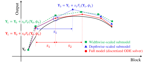
Figure 1: Graph visualization of widthwise/depthwise model scaling inspired by ODE solver.

We propose to scale down the models inspired by solving ODEs in a numerical way (e.g., Euler method). Modern deep neural networks stack residual blocks that contain skip-connections that bypass the residual layers. A residual block is written as $\mathbf{Y}_{j+1}=\mathbf{Y}_{j}+F_{j}(\mathbf{Y}_{j},\phi_{j})$, where $\mathbf{Y}_{j}$ is the feature map at the $j$th layer, $\phi_{j}$ denotes the $j$th block’s network parameters, and $F_{j}$ represents a residual module of the $j$th block. These networks can be interpreted as solving ODEs by numerical analysis (Chang et al., 2018; He et al., 2016).

Consider an initial value problem to find $y$ at $t$ given $\frac{dy}{dt}=f(t,y)$ and $y(t_{0})=y_{0}$. We can obtain $y$ at any point by integration: $y=y_{0}+\int_{t_{0}}^{t}f(t,y)dt$. It can be approximated by Taylor’s expansion as $y=y_{0}+f(t_{0},y_{0})\left(t-t_{0}\right)$ and approximated after more steps as follows:

$$y_{n+1}=y_{n}+hf(t_{n},y_{n})=y_{0}+hf(t_{0},y_{0})+\cdots+hf(t_{n-1},y_{n-1})+hf(t_{n},y_{n}),$$ (1)

where $h$ denotes the step size. An ODE solver can compute with less steps by using larger step size as: $y_{n+1}=y_{0}+2hf(t_{0},y_{0})+\cdots+2hf(t_{n-1},y_{n-1})$ when $n$ is odd. The results would be numerically less accurate than fully computing with a smaller step size. Note that the equation looks like the equation of residual connections. An output of a residual block is rewritten as follows:

$$\mathbf{Y}_{j+1}=\mathbf{Y}_{j}+F_{j}(\mathbf{Y}_{j},\phi_{j})=\mathbf{Y}_{0}+F_{0}(\mathbf{Y}_{0},\phi_{0})+\cdots+F_{j-1}(\mathbf{Y}_{j-1},\phi_{j-1})+F_{j}(\mathbf{Y}_{j},\phi_{j}).$$ (2)

Motivated by this interpreting the neural networks as solving ODEs, we proposed that few residual blocks can be omitted during forward propagation. For example, $\mathbf{Y}_{3}=\mathbf{Y}_{0}+F_{0}+F_{1}+F_{2}$ could be approximated by $\mathbf{Y}_{3}=\mathbf{Y}_{0}+F_{0}+2F_{1}$ omitting the $F_{2}$ block. Here, we propose learnable step size parameters (Touvron et al., 2021; Bachlechner et al., 2021). Instead of pre-determining the step size parameters ($h$’s in the equation (1)), we let step size parameters be trained along with the network parameters. For example, when we omit $F_{2}$ block, output is formulated as $\mathbf{Y}_{3}=\mathbf{Y}_{0}+s_{0}F_{0}+s_{1}F_{1}$ where $s_{i}$’s are also optimized. This enables to scale down the network depthwise. Furthermore, it is also possible to scale each residual block by width (e.g., the size of filters in convolutional layers). The theoretical background behind width-wise scaling is provided by the Eckart-Young-Mirsky theorem (Eckart & Young, 1936). A width-wise scaled residual block represents the optimal $k$-rank approximation of the original (full) block (Horváth et al., 2021).

Our model scaling method inpired by ODE solver is displayed in Figure 1. The black line represents a function to approximate, while the red line represents output approximated by a full nerual netowk. The blue color line represents the depthwise-scaled submodel. The model omitted to compute block $F_{2}(\cdot)$ at the point $\mathbf{Y}_{2}$ and instead, larger step size for computing $F_{1}(\mathbf{Y}_{1},\phi_{1})$ compensates the omitted block (Chang et al., 2018). The green colored line represents the widthwise-scaled submodel that has less parameters $\phi$ in each block. Following the theorem that a widthwise-scaled model with less parameters is an approximation of a model with more parameters (Eckart & Young, 1936), output from a widthwise-scaled model has larger numerical error.

4 NeFL: Nested Federated Learning

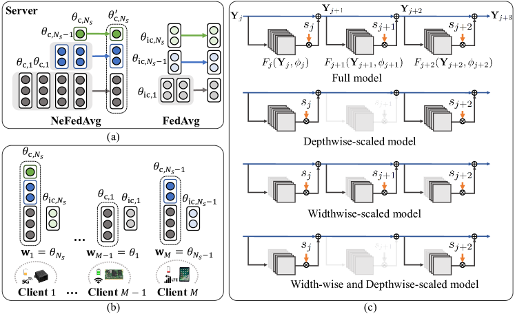
Figure 2: FL with generally split submodels. NeFL aggregates weights of submodels, where the submodels are scaled by both widthwise and depthwise. The weights include consistent and inconsistent parameters.

NeFL is FL framework that accommodates resource-poor clients. Instead of requiring every client to train a single global model, NeFL allows resource-poor clients to train submodels that are scaled in both widthwise and depthwise, based on dynamic nature of their environments. This flexibility enables more clients, even with constrained resources, to pariticipate in the FL pipeline, thereby making the model be trained with a more data. In NeFL pipeline, heterogeneous clients have an ability to determine their submodel at every iteration, allowing them to adapt to varying computing or communication bottlenecks in their respective environments. The NeFL server subsequently aggregates the parameters of these different submodels, resulting in a collaborative and comprehensive global model. Furthermore, during test time, clients have a flexibility to select an appropriate submodel based on their specific background process burdens, such as runtime memory constraints or CPU/GPU bandwidth dynamics. This allows clients to balance between performance and factors like memory usage or latency, tailoring to their individual needs and constraints. To this end, NeFL is twofold: scaling a model into submodels and aggregating the parameters of submodels.

NeFL scales a global model $\mathbf{F}_{G}$ into $N_{s}$ submodels $\mathbf{F}_{1},\dots,\mathbf{F}_{N_{s}}$ with corresponding weights $\theta_{1},\dots,\theta_{N_{s}}$. Without loss of generality, we suppose $\mathbf{F}_{G}=\mathbf{F}_{N_{s}}$. The scaling method is described in following Section 4.1. During each communication round $t$, each client in subset $\mathcal{C}_{t}$ (which is subset of $M$ clients) selects one of the $N_{s}$ submodels based on their respective environments and trains the model by the local epochs $E$. Then, clients transmit their trained weights $\{\mathbf{w}_{i}\}_{i\in\mathcal{C}_{t}}$ to the NeFL server, which aggregates them into $\{\theta_{\textrm{c},N_{s}},\theta_{\textrm{ic},1},\dots\theta_{\textrm{ic},N_{s}}\}$ where $\theta_{\textrm{c},k}$ and $\theta_{\textrm{ic},k}$ denote consistent and inconsistent parameters of a submodel $k$. Note that $\theta_{c,k}\subset\theta_{c,N_{s}}\forall k$. The aggregated weights are then distributed to the clients in $\mathcal{C}_{t+1}$, and this process continues for the total number of communication rounds.

Algorithm 1 NeFL: Nested Federated Learning

Input: Submodels $\{\mathbf{F}_{k}\}_{k=1}^{N_{s}}$, total communication round $T$, the number of local epochs $E$

1:for $t\leftarrow 0$ to $T-1$ do // Global iterations

2:     NeFL server broadcasts the weights $\{\theta_{\textrm{c},N_{s}},\theta_{\textrm{ic},1},\dots\theta_{\textrm{ic},N_{s}}\}$ to clients in $\mathcal{C}_{t}$

3:     $\mathbf{w}_{i}\leftarrow\theta_{j}\in\{\theta_{1},\dots,\theta_{N_{s}}\}$ $\forall i\in\mathcal{C}_{t}$

4:     for $k\leftarrow 0$ to $E-1$ do // Local iterations

5:         Client $i$ updates ${\mathbf{w}_{i}}$ $\forall i\in\mathcal{C}_{t}$      

6:     Client $i$ transmits the weights $\mathbf{w}_{i}$ to the NeFL server $\forall i\in\mathcal{C}_{t}$

7:     $\{\theta_{\textrm{c},N_{s}},\theta_{\textrm{ic},1},\dots\theta_{\textrm{ic},N_{s}}\}\leftarrow\texttt{ParameterAverage}(\{\mathbf{w}_{i}\}_{i\in\mathcal{C}_{t}}$) $\triangleright$ Algorithm 2

4.1 Model Scaling

We propose a global network scaling method, which combines both widthwise scaling and depthwise scaling. We scale the model widthwise by ratio of $\gamma_{W}$ and depthwise by ratio of $\gamma_{D}$. For example, a global model is represented as $\gamma=\gamma_{W}\gamma_{D}=1$ and a submodel that has 25% parameters of a global model can be scaled by $\gamma_{W}=0.5$ and $\gamma_{D}=0.5$. Flexible widthwise/depthwise scaling provides more degree of freedom to split models. We further describe on the scaling strategies in the following sections.

4.1.1 Depthwise Scaling

Residual networks, such as ResNets (He et al., 2016) and ViTs (Dosovitskiy et al., 2021), have gained popularity due to their significant performance improvements on deep networks. The output of a residual block can be seen as a function multiplied by a step size as $\mathbf{Y}_{j+1}=\mathbf{Y}_{j}+s_{j}F(\mathbf{Y}_{j},\phi_{j})=\mathbf{Y}_{0}+\sum_{j}s_{j}F(\mathbf{Y}_{j},\phi_{j})$. Note that ViTs’ forward operation with skip connections can be represented in a similar way by choosing $F(\cdot)$ as either self-attention (SA) layers or feed-forward networks (FFN):

$$\mathbf{Y}_{j+1}=\mathbf{Y}_{j}+s_{j}SA(\mathbf{Y}_{j},\phi_{j}),\quad\mathbf{Y}_{j+2}=\mathbf{Y}_{j+1}+s_{j+1}FFN(\mathbf{Y}_{j+1},\phi_{j+1}).$$

The depthwise scaling can be implemented by skipping any of residual blocks of ResNets or encoder blocks of ViTs. For example, ResNets (e.g., ResNet18, ResNet34) have a downsampling layer followed by residual blocks, each consisting of two convolutional layers. ResNet18 has 8 residual blocks and ResNet34 has 16 residual blocks. ViT/B-16 has 12 encoder blocks where embedding patches are inserted as inputs to following transformer encoder blocks. Each block can have different number of the parameters and computational complexity. A submodel is scaled by omitting few blocks satisfying the number of parameters to be scaled by $\gamma_{D}$ according to system requirements of a client. We can observe that skipping a few blocks in a network still allows it to operate effectively (Chang et al., 2018). This observation is in line with the concept of stochastic depth proposed in (Huang et al., 2016), where a subset of blocks is randomly bypassed during training and the all of the blocks are used during testing.

The step size parameters $s$’s can be viewed as dynamically training how much forward pass should be made at each step. They allow each block to adaptively contribute to useful representations, and larger step sizes are multiplied to blocks that provide valuable information. Referring to Figure 1 and numerical analysis methods (e.g., Euler method, Runge-Kutta methods (Hairer et al., 2000)), adaptive step sizes rather than uniformly spaced steps, can effectively reduce numerical errors. Note that DepthFL (Kim et al., 2023) is a special case of the proposed depthwise scaling.

4.1.2 Widthwise Scaling

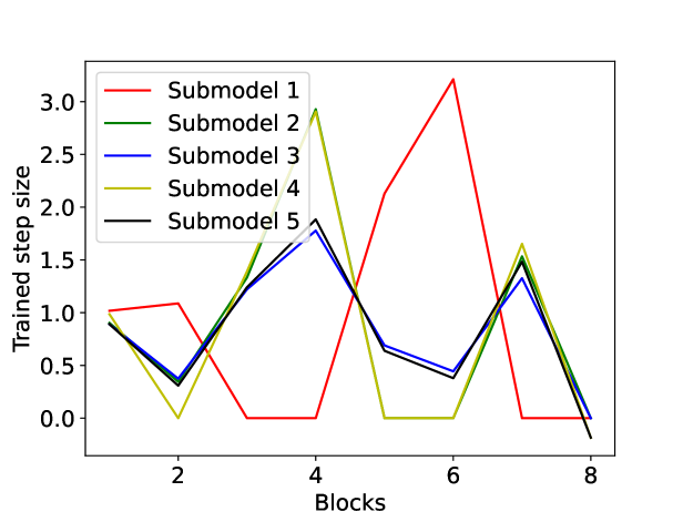
(a) The trained submodels have different step sizes.

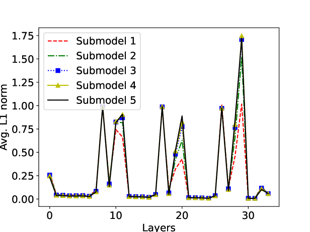
(b) Average L1 norm of weights of submodels trained.

Figure 3: Weights of trained five submodels by NeFL

Previous studies have been conducted on reducing the model size in the width dimension (Li et al., 2017; Liu et al., 2017). In the context of NeFL, widthwise scaling is employed to slim down the network by utilizing structured contiguous pruning (ordered dropout in (Horváth et al., 2021)) along with learnable step sizes. We apply contiguous channel-based pruning to the convolutional networks (He et al., 2017) and node removal to the fully connected layers. The parameters of narrow-width submodel constitute a subset of the parameters of the wide-width model. Consequently, parameters of the slimmest model are trained on any submodel by every client, while the parameters of the larger model is trained less frequently. This approach ensures that the parameters of the slimmest model capture the most of useful representations. Note that each block stated in Section 4.1.1 can have different width, but we suppose throughout the paper that every block has same widthwise scaling ratio $\gamma_{W}$ without loss of generality.

We can obtain further insights from a toy example. Given an optimal linear neural network $y=Ax$ and data from uniform distribution $x\sim\mathcal{X}$, the optimal widthwise-scaled submodel $y=A_{W}x$ is the best $k$-rank approximation by Eckart–Young–Mirsky theorem (Horváth et al., 2021; Eckart & Young, 1936). Given a linear neural network of of rank $k$, widthwise-scaled model of scaling ratio $\gamma_{W}$ has rank of $\lceil\gamma_{W}k\rceil$. Then,

$$\min\mathbb{E}_{x\sim\mathcal{X}}\left\|A_{W}x-Ax\right\|^{2}_{F}=\min\left\|A_{W}-A\right\|^{2}_{F},$$

where $F$ denotes Frobenius norm. In our framework, similar tedency is observed. Inspired by the magnitude-based pruning (Han et al., 2015; Li et al., 2017), we present the L1 norm of weights averaged by the number of weights at each layer of five trained submodels in Figure 3(b). The submodel 1 which is the slimmest model, has similar tendency of L1 norm to the widest model and the gap between submodel gets smaller as the model size gets wider. The slimmest model might have learned the most useful representation while additional parameters for larger models obtain still useful, but less useful information.

4.2 Parameter Averaging

Inconsitency.

NeFL enables training several submodels on local data for subsequent aggregation. However, submodels of different model architectures (i.e., different width and depth) have different characteristics (Acar et al., 2021; Chen et al., 2022; Li et al., 2020b; Santurkar et al., 2018). Referring to Figure 1, if depthwise-scaled model omits a block, it can be compensated by optimizing step size of adjacent blocks. For widthwise-scaled model, numerical errors are induced from each block and they can be mitigated by optimizing step size for each block. We can infer that each submodel requires different step sizes to compensate for the numerical errors according to its respective model architecture. Furthermore, submodels with different model architectures have different loss landscapes. Consider the situation where losses are differentiable. A stationary point of a global model is not necessarily the stationary points of individual submodels (Acar et al., 2021; Li et al., 2020b). Different trainability of neural networks, which varies depending on network architecture, may lead the convergence of submodels to become non-stationary.

The motivation led us to introduce a decoupled set of parameters (Liang et al., 2020; Arivazhagan et al., 2019) for respective submodels that require different parameter averaging method. We refer to these different characteristics between submodels as inconsistency. To this end, we propose the concept of separating a few parameters, referred to as inconsistent parameters, from individual submodels. We address step size parameters and batch normalization layers as inconsistent parameters. Note that batch normalization can improve Lipschitzness of loss, which is sensitive to the convergence of FL (Santurkar et al., 2018; Li et al., 2020c). We further provided an ablation study to assess the effectiveness of inconsistent parameters.

Meanwhile, consistent parameters are averaged across submodels. Since the weights of a submodel are subset of the weights of the largest submodel, the averaging of these weights should be different from conventional FL. The parameters of the submodels are denoted as $\theta_{1}=\{\theta_{{\textrm{c}},1},\theta_{{\textrm{ic}},1}\},\dots,\theta_{N_{s}}=\{\theta_{{\textrm{c}},{N_{s}}},\theta_{{\textrm{ic}},{N_{s}}}\}$ where $\theta_{\textrm{c}}$ denotes consistent parameters and $\theta_{{\textrm{ic}}}$ denotes inconsistent parameters. Note that the global parameters, which are broadcasted to clients for the next FL iteration, encompass $\theta_{{\textrm{c}},N_{s}},\theta_{{\textrm{ic}},{1}},\dots,\theta_{{\textrm{ic}},{N_{s}}}$.

Algorithm 2 ParameterAverage

Input: Trained weights from clients $\mathbf{W}=\{\mathbf{w}_{i}\}_{i\in\mathcal{C}_{t}}$

1:for submodel index $k$ in $\{1,\dots,N_{s}\}$ do

2:     $\mathcal{M}_{k}\leftarrow\{\mathbf{w}_{i}|\mathbf{w}_{i}=\theta_{k}\}_{i\in\mathcal{C}_{t}}$

3:for block $\phi_{j}$ in $\theta_{\textrm{c},N_{s}}$ do // NeFedAvg $\triangleright$ Consistent parameters

4:     $\mathcal{M}^{\prime}\leftarrow\mathcal{M}=\{\mathcal{M}_{k}\}_{k=1}^{N_{s}}$

5:     for $k$ in $\{1,\dots,N_{s}\}$ do

6:         $\mathcal{M}^{\prime}\leftarrow\mathcal{M}^{\prime}\setminus\mathcal{M}_{k}$ if $\phi_{j}\notin\theta_{\textrm{c},k}$      

7:     $k^{\prime}\leftarrow 0$, $\phi_{j,0}=\emptyset$

8:     for $k$ in $\{k|\mathcal{M}_{k}\in\mathcal{M}^{\prime}\}$ do

9:         $\phi_{j,k}\setminus\phi_{j,k^{\prime}}\leftarrow\sum_{\{i|\mathbf{w}_{i}\in\bigcup_{l\geq k,\mathcal{M}_{l}\in\mathcal{M}^{\prime}}\mathcal{M}_{l}\}}{\phi_{j,k}^{i}}\setminus\phi_{j,k^{\prime}}^{i}/\sum_{l\geq k,\mathcal{M}_{l}\in\mathcal{M}^{\prime}}{|\mathcal{M}_{l}|}$

10:         $k^{\prime}\leftarrow k$      

11:$\theta_{\textrm{c},N_{s}}\leftarrow\bigcup_{j}\phi_{j}$

12:for $k$ in $\{1,\dots,N_{s}\}$ do // FedAvg (McMahan et al., 2017) $\triangleright$ Inconsistent parameters

13:     $\theta_{\textrm{ic},k}\leftarrow\sum_{\{i|\mathbf{w}_{i}\in\mathcal{M}_{k}\}}\theta_{\textrm{ic},k}^{i}/|\mathcal{M}_{k}|$

Parameter averaging.

We propose averaging method for the uploaded weights from clients in Algorithm 2. Locally trained weights $\mathbf{W}=\{\mathbf{w}_{i}\}_{i\in\mathcal{C}_{t}}$ from clients are provided as input. The NeFL server verifies which submodel each client’s learned weights correspond to and stores the weights separately by submodel. $\mathcal{M}=\{\mathcal{M}_{1},\dots,\mathcal{M}_{N_{s}}\}$, where $\mathcal{M}_{k}$ denotes weights set from clients who trained $k$-th submodel, is set of uploaded weights sorted by submodels. For consistent parameters, the parameters are averaged by Nested Federated Averaging (NeFedAvg). In short, consistent parameters are averaged in a nested manner. The parameters are averaged by weights from clients who trained the parameters in this round $t$. For nested averaging of parameters, the server accesses parameters block by block since a submodel can have parameters of a block or not. For each block, the server checks which submodel has the block (line 6 in Algorithm 2). Then, parameters are averaged by width in a nested manner. The parameters of a block with the smallest width are included in the parameters of a block with larger width. Hence, the parameters are averaged by weights of clients whose submodels have the block. Meanwhile, the parameters of a block with the largest width is only contained in a submodel that has the largest width. Thus, the parameters are averaged by clients whose submodels have the block with the largest width. For averaging inconsistent parameters, FedAvg (McMahan et al., 2017) is employed. Each submodel has the same size of inconsistent parameters that the inconsistent parameters are averaged for respective submodels. The example for Algorithm 2 is provided in Appendix B.3.

5 Experiments

In this section, we demonstrate the performance of our proposed NeFL over baselines. We provide the experimental results of NeFL that trains submodels from scratch. We also demonstrate whether NeFL aligns with the recently proposed ideas in FL through experiments to verify (i) the performance of NeFL with initial weights loaded from pre-trained model (Chen et al., 2023) and (ii) the performance of NeFL with ViTs in non-IID settings (Qu et al., 2022). We conduct experiments using the CIFAR-10 dataset (Krizhevsky et al., ) for image classification with ResNets and ViTs.

Experimental setup.

The experiments in Table 1 and Table 2 are evaluated with five submodels ($N_{s}=5$ where $\gamma_{1}=0.2,\gamma_{2}=0.4,\gamma_{3}=0.6,\gamma_{4}=0.8,\gamma_{5}=1$) and the experiments in Table 3 are evaluated with three submodels ($N_{s}=3$ where $\gamma_{1}=0.5,\gamma_{2}=0.75,\gamma_{3}=1$). Pre-trained models we use for evaluation are trained on the ImageNet-1k dataset(Deng et al., 2009; Pyt, 2023). The pre-trained weights trained on ImageNet-1k dataset (Deng et al., 2009) are loaded on the initial global models and subsequently NeFL was performed. To take system heterogeneity into account, each client is assigned one of the submodels at each iteration, and statistical heterogeneity was implemented by label distribution skew following the Dirichlet distribution with concentration parameter $0.5$ (Yurochkin et al., 2019; Li et al., 2021a). Training details are provided in Appendix B.1.

Table 1: Results of NeFL for CIFAR-10 dataset under IID (left) and non-IID (right) settings are presented: Top-1 classification accuracies (%) for the worst-case submodel and the average of the performance of five submodels.

Model	Method	IID			non-IID
		Worst	Avg		Worst	Avg
ResNet18	HeteroFL	80.62 ($\pm$ 0.24)	84.26 ($\pm$ 1.95)		76.25 ($\pm$ 1.05)	80.11 ($\pm$ 2.03)
	FjORD	85.12 ($\pm$ 0.22)	87.32 ($\pm$ 1.21)		75.81 ($\pm$ 5.65)	77.99 ($\pm$ 6.50)
	DepthFL	64.80 ($\pm$ 10.49)	82.44 ($\pm$ 10.17)		59.61 ($\pm$ 5.16)	76.89 ($\pm$ 9.60)
	NeFL (ours)	86.86 ($\pm$ 0.22)	87.88 ($\pm$ 0.68)		81.26 ($\pm$ 2.44)	81.71 ($\pm$ 3.14)
ResNet34	HeteroFL	79.51 ($\pm$ 0.44)	83.16 ($\pm$ 1.96)		76.03 ($\pm$ 1.34)	79.63 ($\pm$ 5.24)
	FjORD	85.12 ($\pm$ 0.25)	87.36 ($\pm$ 1.19)		74.70 ($\pm$ 3.66)	76.01 ($\pm$ 5.24)
	DepthFL	25.73 ($\pm$ 4.25)	75.30 ($\pm$ 24.88)		30.42 ($\pm$ 9.34)	70.76 ($\pm$ 21.04)
	NeFL (ours)	87.71 ($\pm$ 0.37)	89.02 ($\pm$ 0.80)		80.76 ($\pm$ 2.82)	83.31 ($\pm$ 2.94)

Table 2: Results of NeFL employing pre-trained models as initial weights for CIFAR-10 dataset under IID (left) and non-IID (right) settings are presented: Top-1 classification accuracies (%) for the worst-case submodel and the average of the performance of five submodels.

Model	Method	IID			non-IID
		Worst	Avg		Worst	Avg
Pre-trained ResNet18	HeteroFL	78.26 ($\pm$ 0.15)	84.48 ($\pm$ 3.04)		71.95 ($\pm$ 1.32)	76.17 ($\pm$ 3.39)
	FjORD	86.37 ($\pm$ 0.18)	88.91 ($\pm$ 1.37)		81.81 ($\pm$ 1.10)	81.96 ($\pm$ 5.76)
	DepthFL	47.76 ($\pm$ 8.54)	82.86 ($\pm$ 17.98)		39.78 ($\pm$ 3.74)	67.71 ($\pm$ 16.88)
	NeFL (ours)	88.61 ($\pm$ 0.08)	89.60 ($\pm$ 0.70)		82.91 ($\pm$ 0.47)	85.85 ($\pm$ 2.43)
Pre-trained ResNet34	HeteroFL	79.97 ($\pm$ 0.53)	84.34 ($\pm$ 2.33)		72.33 ($\pm$ 1.59)	78.2 ($\pm$ 3.29)
	FjORD	87.08 ($\pm$ 0.29)	89.37 ($\pm$ 1.30)		78.2 ($\pm$ 4.39)	78.90 ($\pm$ 6.23)
	DepthFL	52.08 ($\pm$ 5.30)	83.63 ($\pm$ 15.97)		42.09 ($\pm$ 2.79)	79.86 ($\pm$ 18.13)
	NeFL (ours)	88.36 ($\pm$ 0.11)	91.14 ($\pm$ 1.42)		83.62 ($\pm$ 0.68)	86.48 ($\pm$ 2.18)

Table 3: Results of NeFL with three submodels for CIFAR-10 dataset under IID (left) and non-IID (right) settings. A initial weights for global model was given with the pre-trained model with ImageNet-1k. We report Top-1 classification accuracies (%) for the submodels.

Model	Param. #	IID			non-IID
		Worst	Avg		Worst	Avg
Pre-trained ViT	86.4M	93.02 ($\pm$ 0.06)	95.96 ($\pm$ 2.10)		87.56 ($\pm$ 0.16)	92.74 ($\pm$ 3.95)
Pre-trained Wide ResNet101	124.8M	90.9 ($\pm$ 0.16)	91.35 ($\pm$ 0.39)		87.17 ($\pm$ 0.04)	87.74 ($\pm$ 1.06)

Comparison with state-of-the-art model splitting FL methods.

For fair comparison across different baselines, we designed each submodel to have similar number of parameters (Table 8 in Appendix A). As illustrated in Table 1, NeFL outperforms baselines in terms of both the performance of the worst-case submodel ($\gamma=0.2$) and the average performance across five submodels in IID and non-IID settings. Notably, the performance gain is greater in non-IID settings, which belong to practical FL scenarios. It is worth noting that our proposed depthwise scaling method has performance gain over depthwise scaling baselines, while our proposed widthwise scaling method also has performance gain over widthwise scaling baselines (refer to the Appendix A). Furthermore, beyond the performance gain from using depthwise or widthwise scaled submodels, NeFL provides a federated averaging method that can incorporate widthwise or/and depthwise scaled submodels. This characteristic of embracing any submodel with different architecture extracted from a single global model enhances flexibility, enabling more clients to participate in the FL pipeline.

Performance enhancement by employing pre-trained models.

We investigate the performance improvement from incorporating pre-trained models into NeFL and verify that NeFL is still effective when employing pre-trained models. Recent studies on FL have figured out that FL gets benefits from pre-trained models even more than centralized learning (Kolesnikov et al., 2020; Chen et al., 2023). It motivates us to evaluate the performance of NeFL on pre-trained models. The pre-trained model that is trained in a common way using ImageNet-1k is loaded from PyTorch (Paszke et al., 2019). Even when a pre-trained model was trained as a full model without any submodel being trained, NeFL made better performance with these pre-trained models. The results in Table 2 show that the performance of NeFL has been enhanced through pre-training in both IID and non-IID settings following the results of the recent studies. Meanwhile, baselines such as HeteroFL and DepthFL, which do not have any inconsistent parameters, have no effective performance gain when trained with pre-trained models compared to to models trained from scratch.

Impact of model architecture on statistical heterogeneity.

We now present an experiment using ViTs and Wide ResNet (Zagoruyko & Komodakis, 2016) on NeFL. Previous studies have examined the effectiveness of ViTs in FL scenarios, and it has been observed that ViTs can effectively alleviate the adverse effects of statistical heterogeneity due to their inherent robustness to distribution shifts (Qu et al., 2022). Building upon this line of research, Table 3 demonstrates that ViTs outperform ResNets in our framework, with the larger number of parameters, in both IID and non-IID settings. Particularly in non-IID settings, ViTs exhibit less performance degradation of average performance when compared to IID settings. Note that when comparing the performance gap between IID and non-IID settings, the worst-case ViT submodel experiences more degradation than the worst-case ResNet submodel. Nevertheless, despite this degradation, ViT still maintains higher performance than ResNet. Consequently, we verify that ViT on NeFL is also effective following the results in Qu et al. (2022).

Additional experiments.

We provide experimental results of NeFL on other datasets and with different number of clients, along with ablation study in Appendix A. The performance gain of NeFL increases when dealing with more challenging datasets. For example, the performance gain of NeFL with ResNet34 on CIFAR-100 is 7.63% over baselines. We also verify that NeFL shows the best performance across all different number of clients. In our ablation study, we present the effectiveness of inconsistent parameters including learnable step sizes and the performance comparison of proposed scaling methods.

6 Conclusion

In this work, we have introduced Nested Federated Learning (NeFL), a generalized FL framework that addresses the challenges of system heterogeneity. By leveraging proposed depthwise and widthwise scaling, NeFL efficiently divides models into submodels employing the concept of ODE solver, leading to improved performance and enhanced compatibility with resource-constrained clients. We propose to decouple few parameters as inconsistent parameters for respective submodels that FedAvg are employed for averaging inconsistent parameters while NeFedAvg was utilized for averaging consistent parameters. Our experimental results highlight the significant performance gains achieved by NeFL, particularly for the worst-case submodel. Furthermore, we also explore NeFL in line with recent studies of FL such as pretraining and statistical heterogeneity.

Supplementary Material

Appendix A Additional Experiments

A.1 Other Dataset

We evaluate the performance for other dataset such as CIFAR-100 (Krizhevsky et al., ), CINIC-10 (Darlow et al., 2018) SVHN (Netzer et al., 2011) and we observe a similar tendency in terms of Top-1 accuracy of the worst-case submodel and average accuracy over submodels. Note that we set total communication round $T=100$ for training SVHN. The results are presented in Table 4.

Table 4: Results of NeFL with five submodels for CIFAR-100 (left), CINIC10 (center) and SVHN (right) dataset under IID settings. We report Top-1 classification accuracies (%) for the worst-case submodel and the average of the performance of five submodels.

Model	Method	CIFAR-100			CINIC-10			SVHN
		Worst	Avg		Worst	Avg		Worst	Avg
ResNet18	HeteroFL	41.33	47.09		67.55	70.40		91.82	93.46
	FjORD	49.29	52.67		71.95	74.98		94.31	93.97
	DepthFL	31.68	49.56		54.51	71.42		91.54	93.97
	NeFL (ours)	52.63	53.62		74.16	75.29		94.45	94.94
ResNet34	HeteroFL	34.96	39.75		67.39	69.62		89.86	92.39
	FjORD	47.59	50.7		71.58	74.19		93.83	94.63
	DepthFL	14.51	46.79		32.05	67.04		74.33	89.96
	NeFL (ours)	55.22	56.26		75.02	76.68		94.72	95.22

A.2 Different Number of Clients

We conduct further experiments across different numbers of clients. In Table 5, we observe that as the number of clients increases, the performance of NeFL as well as baselines degrades. The results align with previous studies (Kim et al., 2023; Thapa et al., 2022; Wang et al., 2020). The more the number of clients, trained weights deviates further from the weights trained by IID data. While the IID sampling of the training data ensures the stochastic gradient to be an unbiased estimate of the full gradient, the non-IID sampling leads to non-guaranteed convergence and model weight divergence in FL (Li et al., 2020b; 2021b; Zhao et al., 2018). The local clients train their own network with multiple epochs and upload the weights so that the uploaded weights get more deviated. In this regard, our proposed algorithm remains effective across different numbers of clients; however, the performance (e.g., accuracy and convergence) degrades by the data distribution among clients varies more as their number increases.

Table 5: Results of NeFL of five submodels with a global model ResNet18 for CIFAR-10 dataset under IID settings across different number of clients. We report Top-1 classification accuracies (%) for the worst-case submodel and the average of the performance of five submodels..

# of Clients	Model size	Method
		NeFL (ours)	FjORD	HeteroFL	DepthFL
100	Worst	86.86	85.12	80.62	64.8
	Avg	87.88	87.32	84.62	82.44
50	Worst	88.42	86.19	84.67	52.07
	Avg	89.14	88.43	87.23	82.04
20	Worst	89.2	87.76	88.74	24.94
	Avg	89.88	89.6	88.71	76.54

A.3 Ablation Study

Table 6: Ablation study by NeFL with five submodels for CIFAR-10 dataset under IID settings. We report Top-1 classification accuracies (%) for the worst-case submodel and the average of the performance of five submodels.

Model	Method	Worst	Avg
ResNet18	HeteroFL	80.62	84.26
	FjORD	85.12	87.32
	NeFL-W	85.13	87.36
	DepthFL	64.80	82.44
	NeFL-D (N/L)	86.29	88.12
	NeFL-DO (N/L)	86.24	88.22
	NeFL-D	86.06	87.94
	NeFL-DO	85.98	88.20
	NeFL-WD	86.86	87.88
	NeFL-WD (N/L)	86.85	88.21

Model	Method	Worst	Avg
ResNet34	HeteroFL	79.51	83.16
	FjORD	85.12	87.36
	NeFL-W	85.65	87.97
	DepthFL	25.73	75.30
	NeFL-D (N/L)	87.40	89.12
	NeFL-DO (N/L)	86.47	88.49
	NeFL-D	87.71	89.02
	NeFL-DO	87.06	88.71
	NeFL-WD	86.73	88.42
	NeFL-WD (N/L)	86.2	88.16

Model	Method	Worst	Avg
Pre-trained ResNet18	HeteroFL	78.26	84.06
	FjORD	86.37	88.91
	NeFL-W	86.1	89.13
	DepthFL	47.76	82.85
	NeFL-D (N/L)	86.95	89.77
	NeFL-DO (N/L)	86.24	89.76
	NeFL-D	87.13	90.00
	NeFL-DO	87.02	89.72
	NeFL-WD	88.61	89.60
	NeFL-WD (N/L)	88.57	89.70

Model	Method	Worst	Avg
Pre-trained ResNet34	HeteroFL	79.97	84.34
	FjORD	87.08	89.37
	NeFL-W	87.41	89.75
	DepthFL	52.08	83.63
	NeFL-D (N/L)	87.95	90.79
	NeFL-DO (N/L)	87.44	90.58
	NeFL-D	88.36	91.14
	NeFL-DO	87.86	90.90
	NeFL-WD	87.69	90.18
	NeFL-WD (N/L)	87.37	89.78

Model	Method	Worst	Avg
ResNet56	HeteroFL	65.09	74.13
	FjORD	81.38	84.77
	NeFL-W	82.05	85.48
	DepthFL	72.94	86.19
	NeFL-D (N/L)	84.38	86.13
	NeFL-DO (N/L)	83.08	85.59
	NeFL-D	84.38	86.13
	NeFL-DO	81.97	85.37
	NeFL-WD	83.92	86.00
	NeFL-WD (N/L)	83.68	85.85

Model	Method	Worst	Avg
ResNet110	HeteroFL	54.83	67.33
	FjORD	81.70	85.16
	NeFL-W	81.67	85.32
	DepthFL	73.56	82.42
	NeFL-D (N/L)	85.23	86.34
	NeFL-DO (N/L)	84	85.97
	NeFL-D	85.96	86.66
	NeFL-DO	82.74	85.66
	NeFL-WD	84.41	86.28
	NeFL-WD (N/L)	83.58	85.73

For analyzing and experiments for ablation study we refer NeFL-W that all submodels are scaled widthwise, NeFL-D that all submodels are scaled depthwise and NeFL-WD that submodels are scaled both widthwise and depthwise. We further refer to NeFL-D_O that has different initial step sizes with NeFL-D. Referring to Table 13, NeFL-D_O has larger magnitude step sizes aligning with the principles of ODE solver, compared to NeFL-D. NeFL-D scales submodels by skipping a subset of blocks of a global model, thus reducing the depth of the model. NeFL-D does not compensate for the skipped blocks by using larger step sizes. For example, a submodel in NeFL-D is given the initial step sizes as $s_{0}=1,s_{1}=1,s_{2}=0$ and output after Block $2$ without Block $2$ is $\mathbf{Y}_{3}=\mathbf{Y}_{0}+F_{0}+F_{1}$. Meanwhile, NeFL-D_O reduces the size of the global model by skipping a subset of block functions $F(\cdot)$ and gives larger initial step sizes to compensate it. The step sizes are determined based on the number of blocks that are skipped. For a submodel without Block $2$, initial output after Block $2$ is initially computed as $\mathbf{Y}_{3}=\mathbf{Y}_{0}+F_{0}+2F_{1}$ given $s_{0}=1,s_{1}=2,s_{2}=0$. We also refer that submodel with no learnable step sizes by N/L (i.e., constant step sizes are kept with given intial values).

The performance comparison between NeFL-WD and NeFL-WD (N/L) as well as the comparison between NeFL-W and FjORD (Horváth et al., 2021) provides the effectiveness of learnable step sizes and comparison between NeFL-W and HeteroFL (Diao et al., 2021) provides the effectiveness of inconsistent parameters including learnable step sizes. Similarly, the comparison between NeFL-D and NeFL-D (N/L) provides the effectiveness of learnables step sizes and comparison between NeFL-D and DepthFL (Kim et al., 2023) provides the effectiveness of inconsistent parameters including learnable step sizes. We summarized the NeFL with various scaled submodels in Table 7. We also provide the parameter sizes and average FLOPs of submodels by scaling in Table 8.

Referring to the Table 6, the performance improvements of NeFL-WD over NeFL-WD (N/L), NeFL-W over FjORD (Horváth et al., 2021) and NeFL-D over NeFL-D (N/L) provide the effectiveness of learnable step sizes. The effectiveness of the inconsistent parameters including learn step sizes is also verified by NeFL-D over DepthFL (Kim et al., 2023) and NeFL-W over HeteroFL (Diao et al., 2021). We also observe that NeFL-D and NeFL-WD have better performance over widthwise scaling. The performance gap of depthwise scaling over widthwise scaling gets larger for narrow and deep networks. Note that ResNet56 and ResNet110 has smaller (i.e., narrower) channel sizes with more layers (i.e., deeper) than ResNet18 and ResNet34 He et al. (2016). Furthermore, we have a finding that NeFL-D outperforms NeFL-D_O in most cases. The rationale comes from the empirical results that trained step sizes are not as large as initial value for NeFL-D_O that large initial values for NeFL-D_O degrades the trainability of depthwise-scaled submodels.

We evaluated the experiments by similar number of parameters for several scaling methods and depthwise scaling requires slightly more FLOPs than widthwise scaling for ResNet18, ResNet34 and ResNet110 and less FLOPs for ResNet56. Usually depthwise scaled models have more FLOPs than widthwise scaled models while scaling by both widthwise and depthwise models are in between. It is because of the model architecture and limited DoF of submodels. ResNets consist of convolution layers that have FLOPs of the parameters multiplied by feature sizes. The feature sizes get smaller as forwarding the layers and depthwise scaled submodels that omitted the latter layers make a model to require more FLOPs than widthwise scaled submodels that is scaled across all the layers.

It is worth noting that beyond the performance improvement (including that our proposed scaling method NeFL-W and NeFL-D over baselines in Table 6), NeFL provides the more DoF for widthwise/depthwise scaling that can be determined by the requirements of clients. It results in more clients to be participate in the FL pipeline. Also refer to Table 9 that has different scaling ratio $\gamma$. Note that in this case, FjORD (Horváth et al., 2021) outperforms NeFL-W. In this case with severe scaling factors (the worst model has 4% parameters of a global model), step sizes could not compensate the limited number of parameters and degraded the trainability with auxiliary parameters. However, NeFL-WD shows the best performance over other baselines that verify the well-balanced submodels show the better performance than ill-conditioned (too shallow or too narrow) submodels.

Table 7: Summarization of NeFL and baselines for ablation study

	Depthwise scaling	Widthwise scaling	Adaptive step sizes
DepthFL	✓
FjORD, HeteroFL		✓
NeFL-D	✓		✓
NeFL-W		✓	✓
NeFL-WD	✓	✓	✓

Table 8: Details of average FLOPs of submodels of $\bm{\gamma}=[0.2,0.4,0.6,0.8,1]$

Model	Metric	Method
		Width/Depthwise scaling	Widthwise scaling	Depthwise scaling
ResNet18	Param #	6.71M	6.71M	6.68M
	FLOPs	87.8M	85M	102M
ResNet34	Param #	12.6M	12.8M	12.9M
	FLOPs	181M	176M	193M
ResNet56	Param #	0.51M	0.52M	0.51M
	FLOPs	530M	534M	526M
ResNet110	Param #	1.05M	1.06M	1.04M
	FLOPs	158M	159M	234M

Table 9: Results of NeFL with five submodels ($\bm{\gamma}=[0.04,0.16,0.36,0.64,1]$) for CIFAR-10 dataset on ResNet110. Results of NeFL with five submodels for CIFAR-10 dataset under IID settings. We report Top-1 classification accuracies (%) for the worst-case submodel and the average of the performance of five submodels.

Model	Method	Model size
		Worst	Avg
ResNet110	HeteroFL	46.58	63.62
	FjORD	69.61	81.46
	NeFL-W	68.27	80.98
	DepthFL	11.00	53.91
	NeFL-D	75.4	84.31
	NeFL-WD	76.60	84.02

Appendix B Experimental Details

B.1 Training Details

The experiments in Table 1, Table 2, Table 4, Table 5 and Table 6 are evaluated by a total 500 communication rounds ($T$) with 100 clients ($M$). At each round, a fraction rate of $0.1$ is used, indicating that 10 clients ($|\mathcal{C}_{t}|=10$) transmit their weights to the server. During the training process of clients, local batch size of $32$ and a local epoch of $E=5$ are used. For training, we employ SGD optimizer (Ruder, 2016) without momentum and weight decay. The initial learning rate is set to $0.1$ and decreases by a factor of $\frac{1}{10}$ at the halfway point and $\frac{3}{4}$ of the total communication rounds. The experiments in Table 3 are evaluated with the number of clients is $M=10$, all of whom participate in the NeFL pipeline (with a fraction rate of $1$). The experiment consists of $T=100$ communication rounds, and each client performs local training for a single epoch ($E=1$). We use a cosine annealing learning rate scheduling (Loshchilov & Hutter, 2017) with 500 steps of warmup and an initial learning rate 0.03. The input images are resized to a size of $256$ and randomly cropped to a size of $224$ with a padding size of $28$. Note that utilizing layer normalization layers as consistent parameters, as opposed to BN layers that are inconsistent parameters, yields better performance.

B.2 Model Architectures

The ResNet18 architecture and ResNet34 architecture consist of four layers, while ResNet56 and ResNet110 have three layers. These layers are composed of blocks with different channel sizes, specifically (64, 128, 256, 512) for ResNet18/32 and (16, 32, 64) for ResNet56/110. Wide ResNet101_2 comprises four layers of bottleneck blocks with channel sizes (128, 256, 512, 1024) (He et al., 2016; Zagoruyko & Komodakis, 2016). The ViT-B/16 architecture consists of twelve layers, with each layer containing blocks comprising self-attention (SA) and feed-forward networks (FFN) (Dosovitskiy et al., 2021). The widthwise splitting for ViT models are implemented by varying the embedding dimension ($D$ in (Dosovitskiy et al., 2021)).

For the experiments presented in Table 1, Table 2, Table 4, Table 5 and Table 6, we consider five submodels with $\bm{\gamma}=\left[\gamma_{1},\gamma_{2},\gamma_{3},\gamma_{4},\gamma_{5}\right]=\left[0.2,0.4,0.6,0.8,1\right]$ and $\bm{\gamma}=\left[0.04,0.16,0.36,0.64,1\right]$ for Table 9. Additionally, for Table 3, we use three submodels with $\bm{\gamma}=\left[\gamma_{1},\gamma_{2},\gamma_{3}\right]=\left[0.5,0.75,1\right]$. Submodel details for ResNets and ViTs are detailed in Table 10 (ResNet18), Table 11 (ResNet34), Table 13 (ResNet56), Table 15 (ResNet110), Table 15 (Wide ResNet101_2) and Table 13 (ViT-B/16 In the tables, 1’s and 0’s denote the initial values of step sizes. A step size of zero indicates that a submodel does not include the corresponding block. Note that ResNets have a step size parameters for each block while ViTs have different step size parameters to be multiplied with SA and FFN. Submodels in NeFL-W are characterized by $\bm{\gamma}_{D}=[1,\dots,1]$ and $\bm{\gamma}_{W}$ with a target size, while submodels in NeFL-D are characterized by $\bm{\gamma}_{W}=[1,\dots,1]$ and $\bm{\gamma}_{D}$ with a target size. Submodels in NeFL-WD are characterized by target size $\bm{\gamma}_{W}\bm{\gamma}_{D}$. Corresponding number of parameters and FLOPs are provided in Table 8.

B.3 Example on Parameter Averaging

Consider an example with five submodels and suppose that a convolutional layer from the first block is included in submodel 1, 3, and 5. Assume that submodel 1 and submodel 5 are trained twice (two clients), while submodel 3 is trained three times at a communication round. Then, we have $|\mathcal{M}_{2}|=|\mathcal{M}_{4}|=0$, $|\mathcal{M}_{1}|=|\mathcal{M}_{5}|=2$, and $|\mathcal{M}_{3}|=3$. Now, delving into the parameter averaging process, the parameters exclusive to submodel 5 ($\phi_{1,5}\setminus\phi_{1,3}$) are averaged using two updated weights ($\mathcal{M}_{5}$). Likewise, the parameters possessed by submodel 3 but not by submodel 1 ($\phi_{1,3}\setminus\phi_{1,1}$) are averaged using five weights ($\mathcal{M}_{5}\cup\mathcal{M}_{3}$). Finally, the parameters of submodel 1 $\phi_{1,1}$, that is trained seven times, are averaged using seven weights ($\mathcal{M}_{5}\cup\mathcal{M}_{3}\cup\mathcal{M}_{1}$). This approach ensures that consistent parameters are appropriately averaged, taking into account their depthwise inclusion and the widthwise number of occurrences across different submodels.

B.4 Dataset

CIFAR10/100.

The CIFAR10 dataset consists of 60000 images (train dataset consists of 50000 samples and test dataset consists of 10000 samples). $32\times 32\times 3$ color images are categorized by 10 classes, with 6000 images per class (Krizhevsky et al., ). For FL with each client has 500 data samples for $M=100$, and 5000 data samples for $M=10$. We perform data augmentation and pre-processing of random cropping (by $32\times 32$ with padding of 4), random horizontal flip, and normalization by mean of $(0.4914,0.4822,0.4465)$ and standard deviation of $(0.2023,0.1994,0.2010)$.

CINIC10.

The CIFAR10 dataset consists of 270000 $32\times 32\times 3$ color images (train dataset consists of 90000 samples and validation and test dataset consists of 90000 samples respectively) in 10 classes (Darlow et al., 2018). It is constructed from ImageNet and CIFAR10. We perform data augmentation and pre-processing of random cropping (by $32\times 32$ with padding of 4), random horizontal flip, and normalization by mean of $(0.47889522,0.47227842,0.43047404)$ and standard deviation of $(0.24205776,0.23828046,0.25874835)$.

SVHN.

The SVHN dataset consists of 73257 digits for training and 26032 digits for testing of $32\times 32\times 3$ color images (Netzer et al., 2011). The deataset is obtained from house numbers in Google Stree view images in 10 classes (digit ‘0’ to digit ‘9’). For FL for $M=100$ each client has 732 samples. We perform data augmentation and pre-processing of random cropping (by $32\times 32$ with padding of 2), color jitter (by brightness of 63/255, saturation=[0.5, 1.5] and contrast=[0.2, 1.8] implmented by torchvision.transforms.ColorJitter), and normalization by mean of $(0.4376821,0.4437697,0.47280442)$ and standard deviation of $(0.19803012,0.20101562,0.19703614)$.

B.5 Baselines

HeteroFL & FjORD.

HeteroFL (Diao et al., 2021) and FjORD (Horváth et al., 2021) are widthwise splitting methods designed to address the challenges posed by client heterogeneity in FL. While both methods aim to mitigate the impact of heterogeneity, these are several key differences between them. Firstly, HeteroFL does not utilize separate (i.e., inconsistent) parameters for BN layers in its submodels, whereas FjROD incorporates distinct BN layer for each submodel. This difference in handling BN layers can impact the learning dynamics and model performance under IID settings. Secondly, HeteroFL employs static batch normalization, where BN statistics are updated using the entire dataset after the training process. On the other hand, FjORD updates BN statistics during training. Lastly, HeteroFL utilizes a masked cross-entropy loss to address the statistical heterogeneity among clients. This loss function helps to mitigate the impact of clients with the statistical heterogeneity. In our implementation of HeteroFL, the masked cross-entropy loss is not utilized.

DepthFL.

The model is split depthwise, and an auxiliary bottleneck layer is included as an independent classifier. We implement DepthFL (Kim et al., 2023) without separate bottleneck layers for fair comparison without additional parameters. Then, DepthFL is a special case of NeFL-D without inconsistent parameters. Furthermore, due to the accuracy degradation, we omitted knowledge distillation noted in (Kim et al., 2023). Instead, our DepthFL models incorporate downsampling layers that adjust the feature size to match the input sizes of the classifier. It is important to note that the auxiliary bottleneck layers for submodels in DepthFL can be interpreted as parameter decoupling, as discussed in Section 4.2.

B.6 Pre-trained Models

The pre-trained models on Table 2 and Table 3 are trained on ImageNet-1k (Deng et al., 2009) as following recipes (Pyt, 2023):

ResNet18/34.

The models are trained by epochs of 90, batch size of 32, SGD optimizer (Ruder, 2016), learning rate of 0.1 with momentum of 0.9 and weight decay of 0.0001, where learning rate is decreased by a factor of 0.1 every 30 epochs.

Wide ResNet101_2.

The model is trained by epochs of 90, batch size of 32, SGD optimizer (Ruder, 2016), learning rate of 0.1 with momentum of 0.9 and weight decay of 0.0001, where the learning scheduler is cosine learning rate (Loshchilov & Hutter, 2017) and warming up restarts for 256 epochs.

ViT-B/16.

The model is trained by epochs of 300, batch size of 512, AdamW optimizer (Loshchilov & Hutter, 2019) with learning rate of 0.003 and weight decay of 0.3. The learning scheduler is cosine annealing (Loshchilov & Hutter, 2017) after linear warmup method with decay of 0.033 for 30 epochs. Additionally, the random augmentation (Cubuk et al., 2020), random mixup with $\alpha=0.2$ (Zhang et al., 2018), cutmix of $\alpha=1$ (Yun et al., 2019), repeated augmentation, label smoothing of 0.11 (Szegedy et al., 2016), clipping gradient norm to 1, model exponential moving average (EMA) are employed.

B.7 Dynamic Environment

We simulate a dynamic environment by randomly selecting which submodel to be trained by each client during every communication round. In our experiments for Table 1, Table 2, Table 4, Table 5 and Table 6, we have an equal number of five tiers of clients ($M/N_{s}=20$ for all tiers of clients). The resource-constrained clients (tier 1) randomly select models between $\bm{\gamma}=0.2,0.4,0.6$, clients in tier 2 randomly select models from the set $\bm{\gamma}=0.2,0.4,0.6,0.8$, clients in tier 3 randomly select models from the set $\bm{\gamma}=0.2,0.4,0.6,0.8,1$, clients in tier 4 randomly select models from the set $\bm{\gamma}=0.4,0.6,0.8,1$, and the resource-richest clients (tier 5) randomly select models from the set $\bm{\gamma}=0.6,0.8,1$. In our experiments for Table 3 involving three submodels and 10 clients, the tier 1 clients (3 out of 10 total clients) select $\bm{\gamma}=0.5$, tier 2 clients (3 out of 10 total clients) select $\bm{\gamma}=0.75$ and tier 3 clients (4 out of 10 total clients) select $\bm{\gamma}=1$. By allowing clients to randomly choose from the available submodels, our setup reflects the dynamic nature in which clients may encounter communication computing bottlenecks during each iteration.

B.8 Pseudocode for Parameter Averaging

⬇

import numpy as np

\parM = [[] for _ in range(Ns)]

for i in range(len(uploaded_weights)):

for k in range(Ns):

if uploaded_weights[i]==theta[k]: # parameters of submodel k

M[k].append(uploaded_weights[i])

\pardef NeFedAvg(M): # consistent parameters

for block in theta_c[-1]: # global model parameters

for key in block: # depthwise access by block by block

num_submodel_uploaded=[], submodel_idx=[], gamma_W_block=[0]

for k in range(Ns):

if key in theta_c[k]:

submodel_idx.append(k)

num_submodels.append(len(M[k]))

card = np.cumsum(num_submodels[::-1])[::-1] # cardinality

gamma_W_block.append(gamma_W[k])

for i in range(len(submodel_idx)): # widthwise access

start = math.ceil(param_size*gamma_W_block[i])

end = math.ceil(param_size*gamma_W_block[i+1])

for w in M[submodel_idx[i]]:

theta_c_avg[key][start:end]+=w[key][start:end]/card[i]

return theta_c_avg

\pardef InconsistentParamAvg(M): # inconsistent parameters

for k in range(Ns):

for key in theta_ic[k]:

for w in M[k]:

theta_ic_avg[k][key] += w[key]

return theta_ic_avg

Table 10: Details of $\bm{\gamma}$ of NeFL-D and NeFL-WD on ResNet18

Model index	Model size $\gamma$	$\gamma_{W}$	$\gamma_{D}$	NeFL-D (ResNet18)
				Layer 1 (64)	Layer 2 (128)	Layer3 (256)	Layer 4 (512)
1	0.20	1	0.20	1,1	0,0	1,1	0,0
2	0.38	1	0.38	1,0	0,0	1,0	1,0
3	0.57	1	0.57	1,1	1,1	1,1	1,0
4	0.81	1	0.81	1,0	1,1	0,0	1,1
5	1	1	1	1,1	1,1	1, 1	1,1

Model index	Model size $\gamma$	$\gamma_{W}$	$\gamma_{D}$	NeFL-WD (ResNet18)
				Layer 1 (64)	Layer 2 (128)	Layer3 (256)	Layer 4 (512)
1	0.20	0.34	0.58	1,1	1,1	1, 1	1,0
2	0.4	0.4	1	1,1	1,1	1, 1	1,1
3	0.6	0.6	1	1,1	1,1	1, 1	1,1
4	0.8	0.8	1	1,1	1,1	1, 1	1,1
5	1	1	1	1,1	1,1	1, 1	1,1

Table 11: Details of $\bm{\gamma}$ of NeFL-D and NeFL-WD on ResNet34

Model index	Model size $\gamma$	$\gamma_{W}$	$\gamma_{D}$	NeFL-D (ResNet34)
				Layer 1 (64)	Layer 2 (128)	Layer3 (256)	Layer 4 (512)
1	0.23	1	0.23	1,0,0	1,0,0,0	1,0,0,0,0,0	1,0,0
2	0.39	1	0.39	1,1,1	1,1,1,1	1,1,0,0,0,1	1,0,0
3	0.61	1	0.61	1,1,1	1,1,1,1	1,1,0,0,0,1	1,0,1
4	0.81	1	0.81	1,1,1	1,0,0,1	1,1,0,0,0,1	1,1,1
5	1	1	1	1,1,1	1,1,1,1	1,1,1,1,1,1	1,1,1

Model index	Model size $\gamma$	$\gamma_{W}$	$\gamma_{D}$	NeFL-WD (ResNet34)
				Layer 1 (64)	Layer 2 (128)	Layer3 (256)	Layer 4 (512)
1	0.20	0.38	0.53	1,1,1	1,0,0,1	1,0,0,0,0,1	1,0,1
2	0.40	0.63	0.64	1,1,1	1,0,0,1	1,1,1,0,0,1	1,0,1
3	0.60	0.77	0.78	1,1,1	1,1,1,1	1,1,1,1,0,1	1,0,1
4	0.80	0.90	0.89	1,1,1	1,1,1,1	1,1,1,0,0,1	1,1,1
5	1	1	1	1,1,1	1,1,1,1	1,1,1,1,1,1	1,1,1

Table 12: Details of $\bm{\gamma}$ of NeFL-D and NeFL-WD on ResNet56

Model index	Model size $\gamma$	$\gamma_{W}$	$\gamma_{D}$	NeFL-D (ResNet56)
				Layer 1 (16)	Layer 2 (32)	Layer3 (64)
1	0.2	1	0.2	1, 1, 0, 0, 0, 0, 0, 0, 0	1, 1, 0, 0, 0, 0, 0, 0, 0	1, 1, 0, 0, 0, 0, 0, 0, 0
2	0.4	1	0.4	1, 1, 1, 0, 0, 0, 0, 0, 0	1, 1, 1, 0, 0, 0, 0, 0, 0	1, 1, 1, 1, 0, 0, 0, 0, 0
3	0.6	1	0.6	1, 1, 1, 1, 0, 0, 0, 0, 0	1, 1, 1, 1, 0, 0, 0, 0, 0	1, 1, 1, 1, 1, 1, 0, 0, 0
4	0.8	1	0.8	1, 1, 1, 1, 1, 1, 1, 1, 1	1, 1, 1, 1, 1, 1, 1, 1, 0	1, 1, 1, 1, 1, 1, 1, 0, 0
5	1	1	1	1, 1, 1, 1, 1, 1, 1, 1, 1	1, 1, 1, 1, 1, 1, 1, 1, 1	1, 1, 1, 1, 1, 1, 1, 1, 1

Model index	Model size $\gamma$	$\gamma_{W}$	$\gamma_{D}$	NeFL-DO (ResNet56)
				Layer 1 (16)	Layer 2 (32)	Layer3 (64)
1	0.2	1	0.2	1, 8, 0, 0, 0, 0, 0, 0, 0	1, 8, 0, 0, 0, 0, 0, 0, 0	1, 8, 0, 0, 0, 0, 0, 0, 0
2	0.4	1	0.4	1, 1, 7, 0, 0, 0, 0, 0, 0	1, 1, 7, 0, 0, 0, 0, 0, 0	1, 1, 1, 6, 0, 0, 0, 0, 0
3	0.6	1	0.6	1, 1, 1, 6, 0, 0, 0, 0, 0	1, 1, 1, 6, 0, 0, 0, 0, 0	1, 1, 1, 1, 1, 4, 0, 0, 0
4	0.8	1	0.8	1, 1, 1, 1, 1, 1, 1, 1, 1	1, 1, 1, 1, 1, 1, 1, 2, 0	1, 1, 1, 1, 1, 1, 3, 0, 0
5	1	1	1	1, 1, 1, 1, 1, 1, 1, 1, 1	1, 1, 1, 1, 1, 1, 1, 1, 1	1, 1, 1, 1, 1, 1, 1, 1, 1

Model index	Model size $\gamma$	$\gamma_{W}$	$\gamma_{D}$	NeFL-WD (ResNet56)
				Layer 1 (16)	Layer 2 (32)	Layer3 (64)
1	0.2	0.46	0.43	1, 1, 1, 1, 0, 0, 0, 0, 0	1, 1, 1, 1, 0, 0, 0, 0, 0	1, 1, 1, 1, 0, 0, 0, 0, 0
2	0.4	0.61	0.66	1, 1, 1, 1, 1, 1, 0, 0, 0	1, 1, 1, 1, 1, 1, 0, 0, 0	1, 1, 1, 1, 1, 1, 0, 0, 0
3	0.6	0.77	0.77	1, 1, 1, 1, 1, 1, 1, 0, 0	1, 1, 1, 1, 1, 1, 1, 0, 0	1, 1, 1, 1, 1, 1, 1, 0, 0
4	0.8	0.90	89	1, 1, 1, 1, 1, 1, 1, 1, 0	1, 1, 1, 1, 1, 1, 1, 1, 0	1, 1, 1, 1, 1, 1, 1, 1, 0
5	1	1	1	1, 1, 1, 1, 1, 1, 1, 1, 1	1, 1, 1, 1, 1, 1, 1, 1, 1	1, 1, 1, 1, 1, 1, 1, 1, 1

Table 13: Details of $\bm{\gamma}$ of NeFL-D and NeFL-W on ViT-B/16

Model index	Model size $\gamma$	$\gamma_{W}$	$\gamma_{D}$	NeFL-D (ViT-B/16)
				Block
1	0.5	1	0.50	1,1,1,1,1,1,0,0,0,0,0,0
2	0.75	1	0.75	1,1,1,1,1,1,1,1,1,0,0,0
3	1	1	1	1,1,1,1,1,1,1,1,1,1,1,1

Model index	Model size $\gamma$	$\gamma_{W}$	$\gamma_{D}$	NeFL-W (ViT-B/16)
				Block
1	0.5	0.5	1	1,1,1,1,1,1,1,1,1,1,1,1
2	0.75	0.75	1	1,1,1,1,1,1,1,1,1,1,1,1
3	1	1	1	1,1,1,1,1,1,1,1,1,1,1,1

Table 14: Details of $\bm{\gamma}$ of NeFL on ResNet110

Model size $\gamma$	$\gamma_{W}$	$\gamma_{D}$	NeFL-D (ResNet110)
			Layer 1 (16)	Layer 2 (32)	Layer3 (64)
0.2	1	0.20	1, 1, 1, 1, 1, 1, 1, 1, 1, 1, 1, 1, 1, 1, 1, 1, 0, 0	1, 1, 1, 1, 0, 0, 0, 0, 0, 0, 0, 0, 0, 0, 0, 0, 0, 0	1, 1, 1, 0, 0, 0, 0, 0, 0, 0, 0, 0, 0, 0, 0, 0, 0, 0
0.4	1	0.40	1, 1, 1, 1, 1, 1, 1, 1, 1, 1, 1, 1, 1, 1, 0, 0, 0, 0	1, 1, 1, 1, 1, 1, 1, 0, 0, 0, 0, 0, 0, 0, 0, 0, 0, 0	1, 1, 1, 1, 1, 1, 1, 0, 0, 0, 0, 0, 0, 0, 0, 0, 0, 0
0.6	1	0.60	1, 1, 1, 1, 1, 1, 1, 1, 1, 1, 1, 1, 1, 1, 1, 1, 1, 0	1, 1, 1, 1, 1, 1, 1, 1, 1, 1, 1, 1, 1, 0, 0, 0, 0, 0	1, 1, 1, 1, 1, 1, 1, 1, 1, 1, 0, 0, 0, 0, 0, 0, 0, 0
0.8	1	0.80	1, 1, 1, 1, 1, 1, 1, 1, 1, 1, 1, 1, 1, 1, 1, 1, 0, 0	1, 1, 1, 1, 1, 1, 1, 1, 1, 1, 1, 1, 1, 1, 1, 1, 0, 0	1, 1, 1, 1, 1, 1, 1, 1, 1, 1, 1, 1, 1, 1, 0, 0, 0, 0
1	1	1	1, 1, 1, 1, 1, 1, 1, 1, 1, 1, 1, 1, 1, 1, 1, 1, 1, 1	1, 1, 1, 1, 1, 1, 1, 1, 1, 1, 1, 1, 1, 1, 1, 1, 1, 1	1, 1, 1, 1, 1, 1, 1, 1, 1, 1, 1, 1, 1, 1, 1, 1, 1, 1

Model size $\gamma$	$\gamma_{W}$	$\gamma_{D}$	NeFL-WD (ResNet110)
			Layer 1 (16)	Layer 2 (32)	Layer3 (64)
0.2	0.46	0.44	1, 1, 1, 1, 1, 1, 1, 0, 0, 0, 0, 0, 0, 0, 0, 0, 0, 1	1, 1, 1, 1, 1, 1, 1, 0, 0, 0, 0, 0, 0, 0, 0, 0, 0, 1	1, 1, 1, 1, 1, 1, 1, 0, 0, 0, 0, 0, 0, 0, 0, 0, 0, 1
0.4	0.60	0.66	1, 1, 1, 1, 1, 1, 1, 1, 1, 1, 1, 0, 0, 0, 0, 0, 0, 1	1, 1, 1, 1, 1, 1, 1, 1, 1, 1, 1, 0, 0, 0, 0, 0, 0, 1	1, 1, 1, 1, 1, 1, 1, 1, 1, 1, 1, 0, 0, 0, 0, 0, 0, 1
0.6	0.77	0.77	1, 1, 1, 1, 1, 1, 1, 1, 1, 1, 1, 1, 1, 0, 0, 0, 0, 1	1, 1, 1, 1, 1, 1, 1, 1, 1, 1, 1, 1, 1, 0, 0, 0, 0, 1	1, 1, 1, 1, 1, 1, 1, 1, 1, 1, 1, 1, 1, 0, 0, 0, 0, 1
0.8	0.90	0.89	1, 1, 1, 1, 1, 1, 1, 1, 1, 1, 1, 1, 1, 1, 1, 0, 0, 1	1, 1, 1, 1, 1, 1, 1, 1, 1, 1, 1, 1, 1, 1, 1, 0, 0, 1	1, 1, 1, 1, 1, 1, 1, 1, 1, 1, 1, 1, 1, 1, 1, 0, 0, 1
1	1	1	1, 1, 1, 1, 1, 1, 1, 1, 1, 1, 1, 1, 1, 1, 1, 1, 1, 1	1, 1, 1, 1, 1, 1, 1, 1, 1, 1, 1, 1, 1, 1, 1, 1, 1, 1	1, 1, 1, 1, 1, 1, 1, 1, 1, 1, 1, 1, 1, 1, 1, 1, 1, 1

Model size $\gamma$	$\gamma_{W}$	$\gamma_{D}$	NeFL-D (ResNet110)
			Layer 1 (16)	Layer 2 (32)	Layer3 (64)
0.04	1	0.04	1, 0, 0, 0, 0, 0, 0, 0, 0, 0, 0, 0, 0, 0, 0, 0, 0, 0	1, 0, 0, 0, 0, 0, 0, 0, 0, 0, 0, 0, 0, 0, 0, 0, 0, 0	1, 0, 0, 0, 0, 0, 0, 0, 0, 0, 0, 0, 0, 0, 0, 0, 0, 0
0.16	1	0.16	1, 1, 1, 1, 1, 0, 0, 0, 0, 0, 0, 0, 0, 0, 0, 0, 0, 0	1, 1, 1, 0, 0, 0, 0, 0, 0, 0, 0, 0, 0, 0, 0, 0, 0, 0	1, 1, 1, 0, 0, 0, 0, 0, 0, 0, 0, 0, 0, 0, 0, 0, 0, 0
0.36	1	0.37	1, 1, 1, 1, 1, 1, 0, 0, 0, 0, 0, 0, 0, 0, 0, 0, 0, 0	1, 1, 1, 1, 1, 1, 0, 0, 0, 0, 0, 0, 0, 0, 0, 0, 0, 0	1, 1, 1, 1, 1, 1, 1, 0, 0, 0, 0, 0, 0, 0, 0, 0, 0, 0
0.64	1	0.65	1, 1, 1, 1, 1, 1, 1, 1, 1, 1, 1, 0, 0, 0, 0, 0, 0, 0	1, 1, 1, 1, 1, 1, 1, 1, 1, 1, 1, 0, 0, 0, 0, 0, 0, 0	1, 1, 1, 1, 1, 1, 1, 1, 1, 1, 1, 1, 0, 0, 0, 0, 0, 0
1	1	1	1, 1, 1, 1, 1, 1, 1, 1, 1, 1, 1, 1, 1, 1, 1, 1, 1, 1	1, 1, 1, 1, 1, 1, 1, 1, 1, 1, 1, 1, 1, 1, 1, 1, 1, 1	1, 1, 1, 1, 1, 1, 1, 1, 1, 1, 1, 1, 1, 1, 1, 1, 1, 1

Model size $\gamma$	$\gamma_{W}$	$\gamma_{D}$	NeFL-WD (ResNet110)
			Layer 1 (16)	Layer 2 (32)	Layer3 (64)
0.04	0.26	0.16	1, 1, 1, 0, 0, 0, 0, 0, 0, 0, 0, 0, 0, 0, 0, 0, 0, 0	1, 1, 1, 0, 0, 0, 0, 0, 0, 0, 0, 0, 0, 0, 0, 0, 0, 0	1, 1, 1, 0, 0, 0, 0, 0, 0, 0, 0, 0, 0, 0, 0, 0, 0, 0
0.16	0.42	0.38	1, 1, 1, 1, 1, 1, 1, 0, 0, 0, 0, 0, 0, 0, 0, 0, 0, 0	1, 1, 1, 1, 1, 1, 1, 0, 0, 0, 0, 0, 0, 0, 0, 0, 0, 0	1, 1, 1, 1, 1, 1, 1, 0, 0, 0, 0, 0, 0, 0, 0, 0, 0, 0
0.36	0.59	0.61	1, 1, 1, 1, 1, 1, 1, 1, 1, 1, 1, 0, 0, 0, 0, 0, 0, 0	1, 1, 1, 1, 1, 1, 1, 1, 1, 1, 1, 0, 0, 0, 0, 0, 0, 0	1, 1, 1, 1, 1, 1, 1, 1, 1, 1, 1, 0, 0, 0, 0, 0, 0, 0
0.64	0.77	0.83	1, 1, 1, 1, 1, 1, 1, 1, 1, 1, 1, 1, 1, 1, 1, 0, 0, 0	1, 1, 1, 1, 1, 1, 1, 1, 1, 1, 1, 1, 1, 1, 1, 0, 0, 0	1, 1, 1, 1, 1, 1, 1, 1, 1, 1, 1, 1, 1, 1, 1, 0, 0, 0
1	1	1	1, 1, 1, 1, 1, 1, 1, 1, 1, 1, 1, 1, 1, 1, 1, 1, 1, 1	1, 1, 1, 1, 1, 1, 1, 1, 1, 1, 1, 1, 1, 1, 1, 1, 1, 1	1, 1, 1, 1, 1, 1, 1, 1, 1, 1, 1, 1, 1, 1, 1, 1, 1, 1

Table 15: Details of $\bm{\gamma}$ of NeFL on Wide ResNet101_2

Model size $\gamma$	$\gamma_{W}$	$\gamma_{D}$	NeFL-D (Wide ResNet101_2)
			Layer 1 (128)	Layer 2 (256)	Layer3 (512)	Layer 4 (1024)
0.5	1	0.51	1,1,1	1,1,1,1	1, 1, 1, 1, 1, 1, 1, 1, 1, 0, 0, 0, 0, 0, 0, 0, 0, 0, 0, 0, 0, 0, 0	1,1,0
0.75	1	0.75	1,1,1	1,1,1,1	1, 1, 1, 1, 1, 1, 1, 1, 1, 1, 1, 1, 1, 1, 0, 0, 0, 0, 0, 0, 0, 0, 0	1,1,1
1	1	1	1,1,1	1,1,1,1	1, 1, 1, 1, 1, 1, 1, 1, 1, 1, 1, 1, 1, 1, 1, 1, 1, 1, 1, 1, 1, 1, 1	1,1,1

Appendix C Interpreting Scaling with ODE solver

We present a toy example of ODE solvers in Figure 4. The black line representing an actual function is $0.1t+\sin(0.2t)+\cos(0.3t)$ and the red line representing a discretized approximation of the actual function (i.e., a full neural network). Here, it was implemented by ODE solver of step size $h=2$. The green line representing a widthwise scaled submodel has numerical errors on each step. The blue solid line is a depthwise scaled submodel with step size $h=3$. The blue dashed line has forward with same steps, but with optimized step sizes. It denotes that the optimized step sizes can decrease the numerical error. The cyan colored line is implemented by improved Euler method (Hairer et al., 2000) with step size $h=3$. It denotes that even with same steps with blue solid lines, and optimizing $dy/dt$ also contributes to decrease the numerical error. The figure shows a toy example why each submodel can still work well with less parameters.

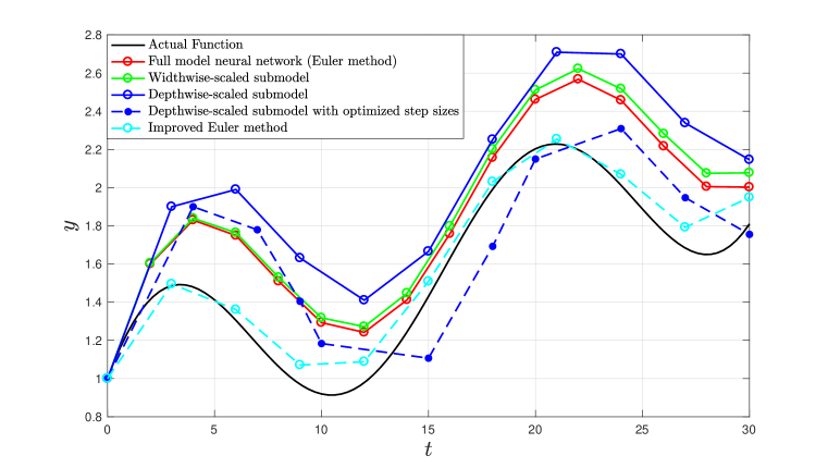
Figure 4: Example of widthwise/depthwise model scaling by ODE solver.

References

- Dat (2022) Data protection: Rules for the protection of personal data inside and outside the EU, 2022. https://commission.europa.eu/law/law-topic/data-protection_en [Accessed: (2023/9/22)].
- Pyt (2023) Pytorch models and pre-trained weights, 2023. https://pytorch.org/vision/stable/models.html [Accessed: (2023/9/22)].
- Acar et al. (2021) Durmus Alp Emre Acar, Yue Zhao, Ramon Matas, Matthew Mattina, Paul Whatmough, and Venkatesh Saligrama. Federated learning based on dynamic regularization. In International Conference on Learning Representations (ICLR), 2021.
- Afonin & Karimireddy (2022) Andrei Afonin and Sai Praneeth Karimireddy. Towards model agnostic federated learning using knowledge distillation. In International Conference on Learning Representations (ICLR), 2022.
- Arivazhagan et al. (2019) Manoj Ghuhan Arivazhagan, Vinay Aggarwal, Aaditya Kumar Singh, and Sunav Choudhary. Federated learning with personalization layers. arXiv preprint arXiv:1912.00818, 2019.
- Bachlechner et al. (2021) Thomas Bachlechner, Bodhisattwa Prasad Majumder, Henry Mao, Gary Cottrell, and Julian McAuley. Rezero is all you need: fast convergence at large depth. In Conference on Uncertainty in Artificial Intelligence (UAI), 2021.
- Buciluǎ et al. (2006) Cristian Buciluǎ, Rich Caruana, and Alexandru Niculescu-Mizil. Model compression. In ACM SIGKDD International Conference on Knowledge Discovery and Data Mining (KDD), 2006.
- Chang et al. (2018) Bo Chang, Lili Meng, Eldad Haber, Frederick Tung, and David Begert. Multi-level residual networks from dynamical systems view. In International Conference on Learning Representations (ICLR), 2018.
- Chen et al. (2023) Hong-You Chen, Cheng-Hao Tu, Ziwei Li, Han Wei Shen, and Wei-Lun Chao. On the importance and applicability of pre-training for federated learning. In International Conference on Learning Representations (ICLR), 2023.
- Chen et al. (2018) Ricky T. Q. Chen, Yulia Rubanova, Jesse Bettencourt, and David Duvenaud. Neural ordinary differential equations. In Advances in Neural Information Processing Systems (NeurIPS), 2018.
- Chen et al. (2022) Xiangning Chen, Cho-Jui Hsieh, and Boqing Gong. When vision transformers outperform resnets without pre-training or strong data augmentations. In International Conference on Learning Representations (ICLR), 2022.
- Cubuk et al. (2020) Ekin Dogus Cubuk, Barret Zoph, Jon Shlens, and Quoc Le. Randaugment: Practical automated data augmentation with a reduced search space. In Advances in Neural Information Processing Systems (NeurIPS), 2020.
- Darlow et al. (2018) Luke N. Darlow, Elliot J. Crowley, Antreas Antoniou, and Amos J. Storkey. Cinic-10 is not imagenet or cifar-10. arXiv preprint arXiv:1810.03505, 2018.
- Deng et al. (2009) Jia Deng, Wei Dong, Richard Socher, Li-Jia Li, Kai Li, and Li Fei-Fei. ImageNet: A large-scale hierarchical image database. In IEEE/CVF Conference on Computer Vision and Pattern Recognition (CVPR), 2009.
- Diao et al. (2021) Enmao Diao, Jie Ding, and Vahid Tarokh. HeteroFL: Computation and communication efficient federated learning for heterogeneous clients. In International Conference on Learning Representations (ICLR), 2021.
- Dosovitskiy et al. (2021) Alexey Dosovitskiy, Lucas Beyer, Alexander Kolesnikov, Dirk Weissenborn, Xiaohua Zhai, Thomas Unterthiner, Mostafa Dehghani, Matthias Minderer, Georg Heigold, Sylvain Gelly, Jakob Uszkoreit, and Neil Houlsby. An image is worth 16x16 words: Transformers for image recognition at scale. In International Conference on Learning Representations (ICLR), 2021.
- Dou et al. (2021) Qi Dou, Tiffany Y So, Meirui Jiang, Quande Liu, Varut Vardhanabhuti, Georgios Kaissis, Zeju Li, Weixin Si, Heather HC Lee, Kevin Yu, et al. Federated deep learning for detecting COVID-19 lung abnormalities in CT: A privacy-preserving multinational validation study. NPJ digital medicine, 4(1):60, 2021.
- Eckart & Young (1936) Carl Eckart and Gale Young. The approximation of one matrix by another of lower rank. Psychometrika, 1(3):211–218, 1936.
- Ha et al. (2017) David Ha, Andrew M. Dai, and Quoc V. Le. Hypernetworks. In International Conference on Learning Representations (ICLR), 2017.
- Haddadpour et al. (2021) Farzin Haddadpour, Mohammad Mahdi Kamani, Aryan Mokhtari, and Mehrdad Mahdavi. Federated learning with compression: Unified analysis and sharp guarantees. In International Conference on Artificial Intelligence and Statistics (AISTATS), 2021.
- Hairer et al. (2000) E. Hairer, S.P. Nørsett, and G. Wanner. Solving Ordinary Differential Equations I Nonstiff problems. Springer, Berlin, second edition, 2000.
- Han et al. (2015) Song Han, Jeff Pool, John Tran, and William J. Dally. Learning both weights and connections for efficient neural networks. In Advances in Neural Information Processing Systems (NeurIPS), 2015.
- He et al. (2020a) Chaoyang He, Murali Annavaram, and Salman Avestimehr. Group knowledge transfer: Federated learning of large cnns at the edge. In Advances in Neural Information Processing Systems (NeurIPS), 2020a.
- He et al. (2020b) Chaoyang He, Murali Annavaram, and Salman Avestimehr. Group knowledge transfer: Federated learning of large cnns at the edge. In Advances in Neural Information Processing Systems (NeurIPS), 2020b.
- He et al. (2021) Chaoyang He, Zhengyu Yang, Erum Mushtaq, Sunwoo Lee, Mahdi Soltanolkotabi, and Salman Avestimehr. SSFL: Tackling label deficiency in federated learning via personalized self-supervision. arXiv preprint arXiv:2110.02470, 2021.
- He et al. (2016) Kaiming He, Xiangyu Zhang, Shaoqing Ren, and Jian Sun. Deep residual learning for image recognition. In IEEE/CVF Conference on Computer Vision and Pattern Recognition (CVPR), 2016.
- He et al. (2017) Yihui He, Xiangyu Zhang, and Jian Sun. Channel pruning for accelerating very deep neural networks. In IEEE International Conference on Computer Vision (ICCV), 2017. doi: 10.1109/ICCV.2017.155.
- Hinton et al. (2015) Geoffrey Hinton, Oriol Vinyals, and Jeff Dean. Distilling the knowledge in a neural network. arXiv preprint arXiv:1503.02531, 2015.
- Hong et al. (2022) Junyuan Hong, Haotao Wang, Zhangyang Wang, and Jiayu Zhou. Efficient split-mix federated learning for on-demand and in-situ customization. In International Conference on Learning Representations (ICLR), 2022.
- Horváth et al. (2021) Samuel Horváth, Stefanos Laskaridis, Mario Almeida, Ilias Leontiadis, Stylianos Venieris, and Nicholas Lane. FjORD: Fair and accurate federated learning under heterogeneous targets with ordered dropout. In Advances in Neural Information Processing Systems (NeurIPS), 2021.
- Huang et al. (2016) Gao Huang, Yu Sun, Zhuang Liu, Daniel Sedra, and Kilian Weinberger. Deep networks with stochastic depth. In European Conference on Computer Vision (ECCV), 2016.
- Jiang et al. (2022) Yuang Jiang, Shiqiang Wang, Víctor Valls, Bong Jun Ko, Wei-Han Lee, Kin K. Leung, and Leandros Tassiulas. Model pruning enables efficient federated learning on edge devices. IEEE Transactions on Neural Networks and Learning Systems (TNNLS), pp. 1–13, 2022.
- Kairouz et al. (2021) Peter Kairouz, H. Brendan McMahan, Brendan Avent, Aurélien Bellet, Mehdi Bennis, Arjun Nitin Bhagoji, Kallista Bonawit, Zachary Charles, Graham Cormode, Rachel Cummings, Rafael G. L. D’Oliveira, Hubert Eichner, Salim El Rouayheb, David Evans, Josh Gardner, Zachary Garrett, Adrià Gascón, Badih Ghazi, Phillip B. Gibbons, Marco Gruteser, Zaid Harchaoui, Chaoyang He, Lie He, Zhouyuan Huo, Ben Hutchinson, Justin Hsu, Martin Jaggi, Tara Javidi, Gauri Joshi, Mikhail Khodak, Jakub Konecný, Aleksandra Korolova, Farinaz Koushanfar, Sanmi Koyejo, Tancrède Lepoint, Yang Liu, Prateek Mittal, Mehryar Mohri, Richard Nock, Ayfer Özgür, Rasmus Pagh, Hang Qi, Daniel Ramage, Ramesh Raskar, Mariana Raykova, Dawn Song, Weikang Song, Sebastian U. Stich, Ziteng Sun, Ananda Theertha Suresh, Florian Tramèr, Praneeth Vepakomma, Jianyu Wang, Li Xiong, Zheng Xu, Qiang Yang, Felix X. Yu, Han Yu, and Sen Zhao. Advances and Open Problems in Federated Learning. Now Foundations and Trends, 2021.
- Kim et al. (2023) Minjae Kim, Sangyoon Yu, Suhyun Kim, and Soo-Mook Moon. DepthFL : Depthwise federated learning for heterogeneous clients. In International Conference on Learning Representations (ICLR), 2023.
- Kolesnikov et al. (2020) Alexander Kolesnikov, Lucas Beyer, Xiaohua Zhai, Joan Puigcerver, Jessica Yung, Sylvain Gelly, and Neil Houlsby. Big transfer (BiT): General visual representation learning. In European Conference on Computer Vision (ECCV), 2020.
- (36) Alex Krizhevsky, Vinod Nair, and Geoffrey Hinton. CIFAR-10 (Canadian Institute for Advanced Research). http://www.cs.toronto.edu/~kriz/cifar.html.
- Lee et al. (2020) Namhoon Lee, Thalaiyasingam Ajanthan, Stephen Gould, and Philip HS Torr. A signal propagation perspective for pruning neural networks at initialization. In International Conference on Learning Representations (ICLR), 2020.
- Li et al. (2017) Hao Li, Asim Kadav, Igor Durdanovic, Hanan Samet, and Hans Peter Graf. Pruning filters for efficient convnets. In International Conference on Learning Representations (ICLR), 2017.
- Li et al. (2021a) Qinbin Li, Yiqun Diao, Quan Chen, and Bingsheng He. Federated learning on non-iid data silos: An experimental study. arXiv preprint arXiv:2102.02079, 2021a.
- Li et al. (2021b) Qinbin Li, Bingsheng He, and Dawn Song. Model-contrastive federated learning. In IEEE/CVF Conference on Computer Vision and Pattern Recognition, 2021b.
- Li et al. (2020a) Tian Li, Anit Kumar Sahu, Ameet Talwalkar, and Virginia Smith. Federated learning: Challenges, methods, and future directions. IEEE Signal Processing Magazine, 37(3):50–60, May 2020a.
- Li et al. (2020b) Tian Li, Anit Kumar Sahu, Manzil Zaheer, Maziar Sanjabi, Ameet Talwalkar, and Virginia Smith. Federated optimization in heterogeneous networks. In Machine Learning and Systems (MLSys), 2020b.
- Li et al. (2020c) Xiang Li, Kaixuan Huang, Wenhao Yang, Shusen Wang, and Zhihua Zhang. On the convergence of fedavg on non-iid data. In International Conference on Learning Representations (ICLR), 2020c.
- Liang et al. (2020) Paul Pu Liang, Terrance Liu, Liu Ziyin, Ruslan Salakhutdinov, and Louis-Philippe Morency. Think locally, act globally: Federated learning with local and global representations. arXiv preprint arXiv:2001.01523, 2020.
- Lin et al. (2020) Tao Lin, Lingjing Kong, Sebastian U Stich, and Martin Jaggi. Ensemble distillation for robust model fusion in federated learning. In Advances in Neural Information Processing Systems (NeurIPS), 2020.
- Liu et al. (2017) Zhuang Liu, Jianguo Li, Zhiqiang Shen, Gao Huang, Shoumeng Yan, and Changshui Zhang. Learning efficient convolutional networks through network slimming. In IEEE International Conference on Computer Vision (ICCV), 2017.
- Loshchilov & Hutter (2017) Ilya Loshchilov and Frank Hutter. SGDR: Stochastic gradient descent with warm restarts. In International Conference on Learning Representations (ICLR), 2017.
- Loshchilov & Hutter (2019) Ilya Loshchilov and Frank Hutter. Decoupled weight decay regularization. In International Conference on Learning Representations (ICLR), 2019.
- Makhija et al. (2022) Disha Makhija, Nhat Ho, and Joydeep Ghosh. Federated self-supervised learning for heterogeneous clients. arXiv preprint arXiv:2205.12493, 2022.
- McMahan et al. (2017) Brendan McMahan, Eider Moore, Daniel Ramage, Seth Hampson, and Blaise Aguera y Arcas. Communication-efficient learning of deep networks from decentralized data. In International Conference on Artificial Intelligence and Statistics (AISTATS), 2017.
- Mugunthan et al. (2022) Vaikkunth Mugunthan, Eric Lin, Vignesh Gokul, Christian Lau, Lalana Kagal, and Steve Pieper. FedLTN: Federated learning for sparse and personalized lottery ticket networks. In European Conference on Computer Vision (ECCV), 2022.
- Netzer et al. (2011) Yuval Netzer, Tao Wang, Adam Coates, Alessandro Bissacco, Bo Wu, and Andrew Y. Ng. Reading digits in natural images with unsupervised feature learning. In NIPS Workshop on Deep Learning and Unsupervised Feature Learning, 2011.
- Paszke et al. (2019) Adam Paszke, Sam Gross, Francisco Massa, Adam Lerer, James Bradbury, Gregory Chanan, Trevor Killeen, Zeming Lin, Natalia Gimelshein, Luca Antiga, Alban Desmaison, Andreas Kopf, Edward Yang, Zachary DeVito, Martin Raison, Alykhan Tejani, Sasank Chilamkurthy, Benoit Steiner, Lu Fang, Junjie Bai, and Soumith Chintala. Pytorch: An imperative style, high-performance deep learning library. In Advances in Neural Information Processing Systems (NeurIPS), 2019.
- Qu et al. (2022) Liangqiong Qu, Yuyin Zhou, Paul Pu Liang, Yingda Xia, Feifei Wang, Ehsan Adeli, Li Fei-Fei, and Daniel Rubin. Rethinking architecture design for tackling data heterogeneity in federated learning. In IEEE/CVF Conference on Computer Vision and Pattern Recognition (CVPR), 2022.
- Rothchild et al. (2020) Daniel Rothchild, Ashwinee Panda, Enayat Ullah, Nikita Ivkin, Ion Stoica, Vladimir Braverman, Joseph Gonzalez, and Raman Arora. FetchSGD: Communication-efficient federated learning with sketching. In International Conference on Machine Learning (ICML), 2020.
- Ruder (2016) Sebastian Ruder. An overview of gradient descent optimization algorithms. arXiv preprint arXiv:1609.04747, 2016.
- Santurkar et al. (2018) Shibani Santurkar, Dimitris Tsipras, Andrew Ilyas, and Aleksander Madry. How does batch normalization help optimization? In Advances in Neural Information Processing Systems (NeurIPS), 2018.
- Seo et al. (2020) Hyowoon Seo, Jihong Park, Seungeun Oh, Mehdi Bennis, and Seong-Lyun Kim. Federated knowledge distillation. arXiv preprint arXiv:2011.02367, 2020.
- Szegedy et al. (2016) Christian Szegedy, Vincent Vanhoucke, Sergey Ioffe, Jon Shlens, and Zbigniew Wojna. Rethinking the inception architecture for computer vision. In IEEE/CVF Conference on Computer Vision and Pattern Recognition (CVPR), pp. 2818–2826, 2016.
- Tan & Le (2019) Mingxing Tan and Quoc Le. EfficientNet: Rethinking model scaling for convolutional neural networks. In International Conference on Machine Learning (ICML), 2019.
- Thapa et al. (2022) Chandra Thapa, Pathum Chamikara Mahawaga Arachchige, Seyit Camtepe, and Lichao Sun. Splitfed: When federated learning meets split learning. AAAI Conference on Artificial Intelligence (AAAI), 2022. doi: 10.1609/aaai.v36i8.20825.
- Touvron et al. (2021) Hugo Touvron, Matthieu Cord, Alexandre Sablayrolles, Gabriel Synnaeve, and Hervé Jégou. Going deeper with image transformers. In IEEE International Conference on Computer Vision (ICCV), 2021.
- Vepakomma et al. (2018) Praneeth Vepakomma, Otkrist Gupta, Tristan Swedish, and Ramesh Raskar. Split learning for health: Distributed deep learning without sharing raw patient data. arXiv preprint arXiv:1812.00564, 2018.
- Wang et al. (2020) Hongyi Wang, Mikhail Yurochkin, Yuekai Sun, Dimitris Papailiopoulos, and Yasaman Khazaeni. Federated learning with matched averaging. In International Conference on Learning Representations (ICLR), 2020.
- Wu et al. (2022) Chuhan Wu, Fangzhao Wu, Lingjuan Lyu, Yongfeng Huang, and Xing Xie. Communication-efficient federated learning via knowledge distillation. Nature Communications, 13(1), Apr. 2022. doi: 10.1038/s41467-022-29763-x.
- Yun et al. (2019) Sangdoo Yun, Dongyoon Han, Seong Joon Oh, Sanghyuk Chun, Junsuk Choe, and Youngjoon Yoo. Cutmix: Regularization strategy to train strong classifiers with localizable features. In IEEE International Conference on Computer Vision (ICCV), 2019.
- Yurochkin et al. (2019) Mikhail Yurochkin, Mayank Agarwal, Soumya Ghosh, Kristjan Greenewald, Nghia Hoang, and Yasaman Khazaeni. Bayesian nonparametric federated learning of neural networks. In International Conference on Machine Learning (ICML), 2019.
- Zagoruyko & Komodakis (2016) Sergey Zagoruyko and Nikos Komodakis. Wide residual networks. In British Machine Vision Conference (BMVC), 2016. ISBN 1-901725-59-6. doi: 10.5244/C.30.87.
- Zhang et al. (2018) Hongyi Zhang, Moustapha Cisse, Yann N. Dauphin, and David Lopez-Paz. mixup: Beyond empirical risk minimization. In International Conference on Learning Representations (ICLR), 2018.
- Zhao et al. (2018) Yue Zhao, Meng Li, Liangzhen Lai, Naveen Suda, Damon Civin, and Vikas Chandra. Federated learning with non-iid data. arXiv preprint arXiv:1806.00582, 2018.
- Zhu et al. (2021) Zhuangdi Zhu, Junyuan Hong, and Jiayu Zhou. Data-free knowledge distillation for heterogeneous federated learning. arXiv preprint arXiv:2105.10056, 2021.
- Zhuang et al. (2022) Weiming Zhuang, Yonggang Wen, and Shuai Zhang. Divergence-aware federated self-supervised learning. In International Conference on Learning Representations (ICLR), 2022.