A Scalable Formal Verification Methodology
for Data-Oblivious Hardware

Abstract

The importance of preventing microarchitectural timing side channels in security-critical applications has surged in recent years. Constant-time programming has emerged as a best-practice technique for preventing the leakage of secret information through timing. It is based on the assumption that the timing of certain basic machine instructions is independent of their respective input data. However, whether or not an instruction satisfies this data-independent timing criterion varies between individual processor microarchitectures.

In this paper, we propose a novel methodology to formally verify data-oblivious behavior in hardware using standard property checking techniques. The proposed methodology is based on an inductive property that enables scalability even to complex out-of-order cores. We show that proving this inductive property is sufficient to exhaustively verify data-obliviousness at the microarchitectural level. In addition, the paper discusses several techniques that can be used to make the verification process easier and faster.

We demonstrate the feasibility of the proposed methodology through case studies on several open-source designs. One case study uncovered a data-dependent timing violation in the extensively verified and highly secure IBEX RISC-V core. In addition to several hardware accelerators and in-order processors, our experiments also include RISC-V BOOM, a complex out-of-order processor, highlighting the scalability of the approach.

I Introduction

In recent years, the view on hardware (HW) as a root-of-trust has been severely damaged. A flood of new security vulnerabilities renewed the focus on microarchitectural side channels. Both software (SW) and HW communities have proposed numerous countermeasures to these new security gaps. However, to fully meet the stringent demands of security-critical applications, a holistic combination of multiple countermeasures is needed that takes consideration of the entire system stack.

The most prominent SW paradigm that tries to mitigate microarchitectural timing side channels is known as data-oblivious, or constant-time, programming [1, 2, 3, 4]. It works by the assumption that the timing and the resource usage of certain operations inside a processor are independent of their respective input data. Constant-time programming is an actively studied discipline with many important contributions from the SW community, including open-source libraries [5, 6, 3], domain-specific languages [7], verification tools [8, 9, 10, 2, 11] and dedicated compilers [12, 13]. The term ”constant-time” can, however, be misleading, as there is no need for execution times to be constant. A variable operation timing is acceptable, as long as it depends only on public information. For example, in constant-time programming, the program itself is considered public information. With this assumption in mind, consider a Read-After-Write (RAW) hazard in a pipelined processor causing a stall. The resulting change in instruction timing is legal because it is based on the public sequence of instructions, not on its (potentially confidential) operands.

The data-oblivious subset of a processor’s instruction set is often referred to as the set of oblivious HW primitives. More complex instructions, which could potentially be insecure, are decomposed into these primitives to ensure a data-oblivious behavior. As a simple example, consider a processor which implements a multi-cycle multiplication. A common optimization in a HW multiplier is to check whether one of the operands is zero and, if so, produce the result after a single cycle. This creates a data-dependent timing and a possible side channel if the operand contains confidential information. Instead of issuing a multiplication, constant-time programming would therefore resort to replacing the multiply instruction by a sequence of primitive instructions like add and shift. However, there is no guarantee that even these simple instructions are actually oblivious HW primitives. Wether or not an instruction fulfills the criterion of data-independent timing can vary between the implemented microarchitectures. Yet, there is only little research on how to verify these assumptions at the microarchitectural level [14, 15, 16, 17].

To make things worse, a recent survey [18] highlighted seven classes of microarchitectural optimizations that all undermine the constant-time paradigm. While exploiting some of these optimizations in commodity processors may seem unrealistic, an attack called Augury [19] demonstrated that this threat is not only a theoretical one. The work shows the security implication of one of these optimizations, namely data memory-dependent prefetchers, as they are present in modern Apple processors. In light of more and more such advanced optimizations being implemented, the question arises as to how we can restore the trust in HW.

To this end, we propose a novel methodology for proving data-oblivious execution of HW operations using standard formal property checking techniques. For processors, the approach certifies a set of trusted HW primitives for data-oblivious programming. Our results show that even simple instructions like a logical shift might suffer from an unexpected timing variability. We also found a potential, and preventable, timing vulnerability in the extensively verified Ibex RISC-V core [20]. Furthermore, we extend the approach to out-of-order cores, demonstrating its feasibility and scalability with an experiment on the Berkeley Out-of-Order Machine (BOOM) [21].

In summary, this paper makes the following contributions:

• Sec. II – We provide a comprehensive overview of related approaches that aim to ensure data-obliviousness building upon an analysis at the HW level.

• Sec. III – We introduce a definition for data-oblivious execution at the microarchitectural level and formalize it using the notion of a 2-safety property over infinite traces. Since most HW designs are not built for data-obliviousness, we also introduce a weaker notion of input-constrained data-obliviousness for general designs. In order to make these properties verifiable in practice, we present how the definitions over infinite traces can be transformed to inductive properties that span over only a single clock cycle.

• Sec. IV – We propose a formal verification methodology, called Unique Program Execution Checking for Data-Independent Timing (UPEC-DIT) [17], that can exhaustively detect any violation of data-obliviousness at the HW level. The methodology is based on standard formal property languages, and can therefore be easily integrated into existing formal verification flows. When applied to processor implementations, UPEC-DIT can be used to qualify the instructions of a microarchitectural ISA implementation regarding their data-obliviousness. These data-oblivious instructions constitute HW primitives for countermeasures such as constant-time programming and can therefore serve as a HW root-of-trust for the higher levels of the system stack.

• Sec. V – We present several optimization techniques, such as black-boxing, proofs over an unrolled model, and cone-of-influence reduction, which can further increase the scalability and usability of the proposed methodology.

• Sec. VI – We demonstrate the feasibility of our approach through case studies on multiple open-source Register-Transfer Level (RTL) designs. Besides several HW accelerators and in-order processors, our experiments also cover the BOOM [21], a superscalar RISC-V processor with floating-point (FP) support, a deep 10-stage pipeline and out-of-order execution.

II Related Work

One of the first works that aims to formally verify data-obliviousness on the microarchitectural level is Clepsydra [14]. In their approach, the authors instrument the HW with Information Flow Tracking (IFT) [22] in such a way that it tracks not only explicit but also implicit timing flows. The verification engineer is then able to perform simulation, emulation or formal verification to verify timing flow properties on the instrumented design. We believe that the ability to utilize a simulation-based approach can be particularly useful when dealing with very large designs. The experiments conducted using formal verification in Clepsydra are, however, restricted to individual functional units, e.g., cryptographic cores. The additional logic added to monitor timing flows introduces a complexity overhead within the design that can be prohibitively large when trying to formally verify data-independent timing in commercial-sized processors.

Other tools that formally verify data-obliviousness at the RTL are XENON [16] and its predecessor IODINE [15]. These tools build their own tool chain and annotation system, utilizing open-source libraries and special-purpose solvers. While this approach is an important contribution to restoring trust in HW, its dependency on special-purpose solvers may be an obstacle to adoption in industry. In contrast, in our proposed methodology, we use standard SystemVerilog Assertions (SVA) combined with state-of-the-art SAT-based formal property checking tools. Our goal is to complement existing formal workflows, creating a synergy between functional and security verification. Furthermore, although XENON makes significant performance improvements over its predecessor, it may face complexity hurdles when dealing with commercial microarchitectures. With the work proposed in this paper, we aim to significantly improve the scalability of formal security verification and, for the first time, present a method that is applicable to large processors featuring out-of-order execution.

A related line of research aims to establish a formally defined relationship between HW and SW by formulating and verifying so-called HW/SW contracts [23]. Similar to [17], they can be used to prove data-independent timing on an instruction-level granularity. However, current experiments only cover in-order processor designs up to a pipeline depth of three stages. A promising and ongoing related work named TransmitSynth [24, 25] maps such a contract to a verifiable SVA property in order to automatically detect data-dependent side effects. TransmitSynth can enumerate microarchitectural execution paths for a given instruction under verification. This allows for a fine-grained categorization of leakage scenarios. However, the workflow includes a manual annotation of so-called Performing Locations (PLs), which are identifiers that mark an instruction execution path. Correctly marking these PLs requires some knowledge of the underlying design and could be increasingly difficult with more complex systems, especially for deep out-of-order processors like BOOM.

Other work pursues augmenting the Instruction Set Architecture (ISA) with information about the data-obliviousness of instructions. In fact, both Intel [26] and ARM [27] have recently added support for instructions with data-independent timing. With the same goal in mind, RISC-V [28] has just ratified the Cryptography Extension for Scalar & Entropy Source Instructions [29]. A subset of this extension, denoted Zkt, requires a processor to implement certain instructions of standard extensions with a data-independent execution latency. This ISA contract provides the programmer with a safe subset of instructions that can be used for constant-time programming. Another work on a Data-Oblivious ISA Extension (OISA) [30, 31] proposes to refine the ISA with information about the data-obliviousness of each instruction. The authors then develop hardware support for this to track wether confidential information can reach unsafe operands. The method proposed here is complementary to the research efforts on such architectures as it provides a tool to verify their security.

III Theoretical Foundation

In this section, we introduce a formal notation that we will use throughout this paper (Sec. III-A). We formally define data-obliviousness at the microarchitectural level (Sec. III-B) and then develop a weaker definition that is suitable for general circuits not specifically designed for data-obliviousness (Sec. III-C). In order to ensure scalability for more complex designs, we translate these definitions, which are formulated over infinite traces, into 1-cycle inductive properties (Sec. III-D). We prove that these inductive properties are equivalent to the corresponding definitions over infinite traces. To conclude this chapter, we address some interesting special cases (Sec. III-E).

III-A Definitions

We first introduce some general notations to reason about data-obliviousness as a HW property. We model a digital HW design as a standard finite state machine (FSM) of Mealy type, $M=(I,S,S_{0},O,\delta,\lambda)$, with finite sets of input symbols $I$, output symbols $O$, states $S$, initial states $S_{0}\subseteq S$, transition function $\delta:S\times I\mapsto S$ and output function $\lambda:S\times I\mapsto O$. The interface sets $I$, $O$ and the state set $S$ are encoded in (binary-valued) input variables $X$, output variables $Y$ and state variables $Z$, respectively.

A key observation is that, in a HW design, the timing of a module is dictated by its control behavior. Accordingly, we partition each interface set into two disjoint subsets in order to separate control ($C$) from data ($D$). We denote these sets as $X_{C}$, $X_{D}$, $Y_{C}$ and $Y_{D}$, with

$$X_{C}\cup X_{D}=X;X_{C}\cap X_{D}=\emptyset$$

$$Y_{C}\cup Y_{D}=Y;Y_{C}\cap Y_{D}=\emptyset$$

In practice, this partitioning of the interface is straightforward and is usually done manually based on the specification of the design. For example, the operands and the result of a functional unit are considered data, whereas any handshaking signals that trigger the start of a new computation or indicate that a provided result is valid belong to control.

We further define a trace $\tau=\{e_{0},e_{1},...\}$ to be a sequence of events, with an event $e_{t}$ being a tuple $(i_{t},s_{t},o_{t})$, where $i_{t}$ is the valuation of our design’s input variables $X$ at time point (clock cycle) $t$, $s_{t}$ is its state, as represented by the value of $Z$ at $t$ and $o_{t}$ is the valuation of its output variables $Y$ at $t$. Let $T$ be the set of all infinite traces of the design where $s_{0}\in S_{0}$.

We introduce the following definitions:

• $s(\tau)=\{s_{0},s_{1},...\}$ is the sequence of valuations to the design’s state variables $Z$ in the trace $\tau\in T$.

• $i(\tau)=\{i_{0},i_{1},...\}$ is the sequence of valuations to the design’s input variables $X$ in the trace $\tau\in T$. Likewise, $i_{C}(\tau)$ is the sequence of valuations to $X_{C}$ and $i_{D}(\tau)$ is the sequence of valuations to $X_{D}$.

• $o(\tau)=\{o_{0},o_{1},...\}$ is the sequence of valuations to the design’s output variables $Y$ in the trace $\tau\in T$. Likewise, $o_{C}(\tau)$ is the sequence of valuations to $Y_{C}$ and $o_{D}(\tau)$ is the sequence of valuations to $Y_{D}$.

• With a slight abuse of notation, we also allow the above functions to take single events as arguments, e.g., $s(e_{t})=s_{t}$.

• For any $t\in\mathbb{N}_{0}$, the notation $\tau[t]$ represents the event $e_{t}$ at time point $t$. For example, $s(\tau[t])=s_{t}$ represents the valuation to the state variables in $Z$ at time point $t$.

• Similarly, we define the notion $[t..]$ as an infinite time interval beginning with and including $t$. Accordingly, $\tau[t..]$ represents an infinite subsequence of $\tau$ that starts at and includes the time point $t$.

III-B Data-Obliviousness in HW

Having established a basic notation, we proceed to defining data-oblivious behavior at the microarchitectural level. In our threat model, we assume that an attacker cannot access confidential information directly. The attacker is, however, able to observe the control signals of the design under attack, e.g., by monitoring bus transactions. This means that, for a HW module to be data-oblivious, the data used in the computations must not affect the operating time or cause other microarchitectural side effects. Based on this intuition we formulate a definition of the security feature under verification:

Definition 1 (Data-Obliviousness).

A HW module is called Data-Oblivious (DO) if the sequence of values of its control outputs $Y_{C}$ is uniquely determined by the sequence of values at the control inputs $X_{C}$. ∎

We can express Def. 1 formally as a 2-safety property over infinite traces. We formalize it as follows: For any two infinite traces running on the design whose starting states at time $t$ are identical and which receive the same control input sequences from time point $t$ on, data-obliviousness guarantees that the control outputs after $t$ are also identical:

$$\begin{split}\textit{{DO}}\coloneq\ &\forall\tau_{1},\tau_{2}\in T,\ \forall t\in\mathbb{N}_{0}:\\ &s(\tau_{1}[t])=s(\tau_{2}[t])\land i_{C}(\tau_{1}[t..])=i_{C}(\tau_{2}[t..])\\ &\Rightarrow o_{C}(\tau_{1}[t..])=o_{C}(\tau_{2}[t..])\end{split}$$ (1)

III-C Input-Constrained Data-Obliviousness

Def. 1 of data-obliviousness is fairly straightforward. Put simply, it ensures that the control behavior of a HW design is independent of the data it processes. Unfortunately, this strict definition works only for HW that is carefully designed for data-obliviousness. In general, however, designs are not data-oblivious. A processor must be able to make decisions based on the data it is processing, for example, when it executes conditional branch instructions. Constant-time programming tries to prevent data-dependent timing by excluding such instructions from the security-critical parts of the program. Data-obliviousness is achieved by restricting the program to only use a data-oblivious subset of the ISA. Consequently, in order to qualify a microarchitectural implementation for data-obliviousness, we require a separation between data-oblivious and non-data-oblivious operations at the HW level. This means, we must systematically identify and formally verify the control input configurations under which the design operates data-independently. In practice, this requires constraining the possible input values to a legal subset that ensures data-obliviousness.

Definition 2 (Input-constrained Execution).

An input constraint is a non-empty subset $\phi\subseteq I$ of the possible inputs to the design. An input-constrained trace $\tau_{\phi}$ is an infinite trace in which the inputs to the design are constrained by $\phi$, i.e., $i(\tau_{\phi}[t])\in\phi$ for every $t\in\mathbb{N}$. The subset $T_{\phi}\subseteq T$ of all traces constrained by $\phi$ is called input-constrained execution of the design. ∎

We can now modify Def. 1 to introduce a weaker notion of data-obliviousness. We call a HW design that provides a data-oblivious subset of its functionality input-constrained data-oblivious.

Definition 3 (Input-constrained Data-Obliviousness).

A HW design is called input-constrained data-oblivious ($DO_{\phi}$) if, for a given input constraint $\phi\subseteq I$, the values of its control outputs $Y_{C}$ are uniquely determined by the sequence of control inputs $X_{C}$. ∎

In essence, Def. 3 partitions the design behavior into data-oblivious and non-oblivious HW operations. The HW runs without any observable side effect on the architectural level, as long as only inputs within the constraint $\phi$ are given. For the special case of $\phi=I$, Def. 3 is equivalent to the original Def. 1.

As an example, assume a processor executing a sequence of instructions. If each instruction is a data-oblivious HW primitive, e.g., an addition or a logic operation whose execution time is data-independent (as in most microarchitectures), the sequence of instructions as a whole is also data-oblivious. However, if an instruction has a data-dependent behavior, e.g., a variable-time division, the entire sequence of instructions becomes non-oblivious. We use a constraint $\phi$ to exclude such an instruction from consideration. The goal of the proposed methodology is to systematically find all scenarios that cause data-dependent side effects.

The following trace property formalizes the requirement of input-constrained data-obliviousness:

$$\begin{split}\textit{{DO}}_{\phi}\coloneq\ &\exists\phi,\ \forall\tau_{1},\tau_{2}\in T_{\phi},\ \forall t\in\mathbb{N}_{0}:\\ &s(\tau_{1}[t])=s(\tau_{2}[t])\land i_{C}(\tau_{1}[t..])=i_{C}(\tau_{2}[t..])\\ &\Rightarrow o_{C}(\tau_{1}[t..])=o_{C}(\tau_{2}[t..])\end{split}$$ (2)

III-D Formally Proving Data-Obliviousness in Practice

In the previous subsections, we defined data-obliviousness as a property over infinite traces. Most commercial model checking tools, however, reason about sequential circuits by unrolling the combinatorial part of the design over a finite number of clock cycles. Therefore, our definitions of data-obliviousness formalized over an infinite number of clock cycles are not yet suitable for being checked on practical tools.

For exhaustive coverage of every possible design behavior, the circuit must be unrolled to its sequential depth. The sequential depth of a circuit is the minimum number of clock cycles needed to reach all possible states, typically starting from the reset state of the design. For most practical designs, the sequential depth can easily reach thousands of clock cycles. To make things worse, the sheer size of an industrial design may make it impossible for the property checker to unroll for more than a few clock cycles, even for highly optimized commercial tools. Therefore, it is usually not possible to verify such a design exhaustively with bounded model checking from the reset state.

Interval Property Checking (IPC) [32, 33] provides unbounded proofs and can scale to large designs by starting from a symbolic initial state. Instead of traversing a large number of states from reset, IPC starts from an arbitrary “any” state. However, there are two challenges associated with this approach.

The first challenge stems from the nature of the symbolic initial state. Since the proof starts from any possible state, it also includes states that are unreachable from reset. This can lead to false counterexamples, since the property in question may hold for the set of reachable states, but fail for certain unreachable states. This challenge arises not only in security verification, but in all formal verification approaches that use a symbolic initial state. A standard approach to address this problem is to add invariants to the proof:

Definition 4 (Invariant).

For a given HW design, we call a subset of states $B\subseteq S$ an invariant if for every state $s\in B$ all its successor states $s^{\prime}$ are also in $B$. This means that,

$$\forall s\in S,\forall i\in I:s\in B\Rightarrow\delta(s,i)\in B$$

∎

In other words, an invariant is a set of states that is closed under reachability. To simplify the notation, we implicitly assume that $S_{0}\subseteq B$ in the rest of the paper, i.e., we only consider invariants that include the reset states.

Even when using a symbolic initial state that “fast-forwards” the system to an arbitrary execution state, the data must still propagate from the input through the system before it can affect a control output. Therefore, the second challenge is to handle the structural depth, i.e., the length of the propagation path from $X_{D}$ to $Y_{C}$, of the design. For large and complex designs, unrolling the circuit is costly and quickly reaches the capacity of formal tools. In such cases, it is not possible to make exhaustive statements about a design’s data-obliviousness based on its I/O behavior alone and we need to look into the internal state of the system.

For this problem, we propose an inductive property for data-obliviousness that spans a single clock cycle and that also considers internal state signals. Just like for the input/output signals, we partition the set of state variables $Z$ into control variables $Z_{C}$ and data variables $Z_{D}$, where $Z_{C}\cup Z_{D}=Z$ and $Z_{C}\cap Z_{D}=\emptyset$. Accordingly, $s_{C}(\tau)$ is the sequence of valuations to $Z_{C}$ and $s_{D}(\tau)$ is the sequence of valuations to $Z_{D}$. For the sake of a simplified notation, we also let $i_{C}$, $o_{C}$ and $s_{C}$ take an input symbol, output symbol or state of the Mealy machine and return the valuation of the corresponding subset of control signals $X_{C}$, $Y_{C}$ and $Z_{C}$, respectively. We present how to systematically partition $Z$ into $Z_{C}$ and $Z_{D}$ later in Sec. IV such that this process is always conservative in terms of security.

The data-obliviousness property that we use as an element of our inductive reasoning is shown in Eq. 3.

$$\begin{split}\textit{{DO'}}\coloneq\ &\exists B\subseteq S,\ \forall s_{1},s_{2}\in B,\ \forall i_{1},i_{2}\in I:\\ &s_{C}(s_{1})=s_{C}(s_{2})\land i_{C}(i_{1})=i_{C}(i_{2})\\ &\Rightarrow s_{C}(\delta(s_{1},i_{1}))=s_{C}(\delta(s_{2},i_{2}))\\ &\land o_{C}(\lambda(s_{1},i_{1}))=o_{C}(\lambda(s_{2},i_{2}))\end{split}$$ (3)

This property expresses that if we have two instances of the system for which the control inputs and states have equal values, then the control state variables will also be equal in the next states of the two instances. This weakens the initial assumption that a discrepancy between the two instances can originate only from the data inputs. By allowing internal data (state) signals to take arbitrary values, we implicitly model any propagation of data through the system by the symbolic initial state.

It is important to remember that the invariant $B$ is a superset of the reachable states because we require it to include the initial states, $S_{0}\subseteq B$. In practice, the security property of Eq. 3 holds not only in the reachable state set but, often, also in many unreachable states. Therefore, finding a suitable invariant for the given property is usually less of a problem than may be generally expected. In our proposed methodology (Sec. IV), we systematically create the necessary invariant in an iterative procedure and prove it on the fly along with the property for data-obliviousness.

In the same way as for Eq. 3, we can derive an inductive property for data-obliviousness when the set of allowed inputs to the design is restricted by a constraint $\phi$ (Def. 3). This causes a restriction also in the set of reachable states, which must be expressed by an invariant. To this end, we extend Def. 4 and denote $B_{\phi}$ as a set of states for which $\forall s\in S,\forall i\in\phi:s\in B_{\phi}\Rightarrow\delta(s,i)\in B_{\phi}$ under a given constraint $\phi$. As an example, assume that the input constraint $\phi$ excludes branch instructions from entering the pipeline of our processor. A corresponding invariant $B_{\phi}$ excludes all states that involve processing of such branch instructions. We elaborate on how to systematically derive such an invariant in Sec. IV.

Eq. 4 shows the inductive property for input-constrained data-obliviousness.

$$\begin{split}\textit{{DO'}}_{\phi}\coloneq\ &\exists\phi,\ \exists B_{\phi}\subseteq S,\ \forall s_{1},s_{2}\in B_{\phi},\ \forall i_{1},i_{2}\in\phi:\\ &s_{C}(s_{1})=s_{C}(s_{2})\land i_{C}(i_{1})=i_{C}(i_{2})\\ &\Rightarrow s_{C}(\delta(s_{1},i_{1}))=s_{C}(\delta(s_{2},i_{2}))\\ &\land o_{C}(\lambda(s_{1},i_{1}))=o_{C}(\lambda(s_{2},i_{2}))\end{split}$$ (4)

We now show that, for any HW design, our inductive properties cover their corresponding definitions over infinite traces.

Theorem 1 ((3) $\Rightarrow$ (1) and (4) $\Rightarrow$ (2)).

If a HW design operates (constrained) data-obliviously according to the inductive property Eq. 3 (Eq. 4), it also operates (constrained) data-obliviously according to the property over infinite traces Eq. 1 (Eq. 2).

Proof.

We show that (4) $\Rightarrow$ (2). This covers (3) $\Rightarrow$ (1) for the special case that $\phi=I$.  
We prove this implication by contradiction. Assume a HW design fulfills property (4) for a given $\phi$ but violates property (2), i.e., there exists a set of traces $\tau_{1},\tau_{2}\in T_{\phi}$ with $t\in\mathbb{N}_{0}:s(\tau_{1}[t])=s(\tau_{2}[t])\land i_{C}(\tau_{1}[t..])=i_{C}(\tau_{2}[t..])$ such that $\exists t_{k}\in\mathbb{N}_{0}:o_{C}(\tau_{1}[t_{k}])\neq o_{C}(\tau_{2}[t_{k}])$ where $t_{k}>t$. (The case $t_{k}=t$ can be excluded since property (4) holds on the design and $Z_{C}\subseteq Z$.)

$o_{C}(\tau_{1}[t_{k}])\neq o_{C}(\tau_{2}[t_{k}])$ requires that the antecedent of (4) is violated at time point $t_{k}-1$. Since our initial assumption requires $i_{C}(\tau_{1}[t_{k}-1])=i_{C}(\tau_{2}[t_{k}-1])$, it follows that $s_{C}(\tau_{1}[t_{k}-1])\neq s_{C}(\tau_{2}[t_{k}-1])$. However, this is a contradiction to

$$\begin{split}s(\tau_{1}[t])=s(\tau_{2}[t])\overset{Z_{C}\subseteq Z}{\Rightarrow}&s_{C}(\tau_{1}[t])=s_{C}(\tau_{2}[t])\\ \overset{(\ref{eq:cdo-1-cycle})}{\Rightarrow}\ \ &s_{C}(\tau_{1}[t+1])=s_{C}(\tau_{2}[t+1])\\ \overset{(\ref{eq:cdo-1-cycle})}{\Rightarrow}...\overset{(\ref{eq:cdo-1-cycle})}{\Rightarrow}\ \ &s_{C}(\tau_{1}[t_{k}-1])=s_{C}(\tau_{2}[t_{k}-1])\end{split}$$

which means that our initial assumption is wrong, and therefore (4) $\Rightarrow$ (2). ∎

Proving the relationship ”(4) $\Rightarrow$ (2)” is crucial to ensure the validity of our proposed approach. If we can verify the inductive property on the design, we have also verified that the property over infinite traces holds. Our approach requires us to find some system invariant for which the inductive property holds. Usually, in practice, such an invariant can include the majority of the unreachable states. This is key to the feasibility of the proposed methodology, as it makes finding a suitable invariant much more practical.

The implication in the opposite direction, i.e., ”(2) $\Rightarrow$ (4)”, is not true for the general case. The reason for this is that Eq. 4 can over-approximate the state space, which could lead to false counterexamples. However, this does not affect the validity of the proposed methodology, as its goal is to prove the inductive property.

III-E Special Cases

In Def. 1, we model the security-critical timing behavior by a set of control output signals, e.g., signals responsible for bus handshaking. The concern might arise as to how these properties can be formulated if the design under verification does not implement any such control interface at all. The question is: What is a realistic attacker model in this case? If an attacker can observe the data outputs themselves, any constant-time provisions are futile. If we assume a scenario, in which the attacker can spy on internal signals to determine when an operation has finished, we can prove data-independence for these signals instead. In any case, if there is no handshaking control implemented whatsoever, the specification must give detailed information about the timing behavior of the system. Then, timing is an essential part of the circuit’s functional correctness and should be covered by conventional verification methods.

IV Methodology

In this chapter, we present Unique Program Execution Checking for Data-Independent Timing (UPEC-DIT) building upon earlier work in [17]. UPEC-DIT is a formal methodology to systematically and exhaustively detect data-dependent behavior at the microarchitectural level. In particular, we show how UPEC-DIT is used to verify data-obliviousness by proving the properties introduced in the previous chapter (Eq. 3 and Eq. 4). In the following, for reasons of simplicity, when the distinction between the case of $\phi=I$ and the case of $\phi\subset I$ is irrelevant, we omit the term ”input-constrained” and simply speak of ”data-obliviousness”.

IV-A UPEC-DIT Overview

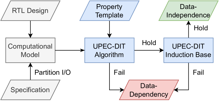
Figure 1: UPEC-DIT Flow

Fig. 1 shows an overview of the different steps of the methodology. We describe each step in more detail in the following subsections. We base our work on a methodology called Unique Program Execution Checking (UPEC) [34, 35]. UPEC utilizes IPC [32, 33] and a 2-safety model to systematically and exhaustively trace the propagation of confidential information through the system. Originally, UPEC was devised to detect transient execution attacks in processors. In that scenario, the secret is stored at a protected location (data-at-rest) from which it must never leak into the architecturally visible state.

This paper extends over previous UPEC approaches in that it targets a threat model for data-in-transit, i.e., confidential information is processed legally, but must not cause any unwanted side effects.

Our starting point is the RTL description of the system. Based on the specification, we partition the I/O signals of the design into control and data. With this information, we create the computational model and initialize the main inductive property for UPEC-DIT which is then submitted to the main algorithm that implements the induction step in our global reasoning. During the execution of the algorithm, the property is iteratively refined with respect to the internal state signals until it either holds or a counterexample is returned, describing a data-dependent behavior. This refinement procedure is conservative in the sense that a wrong decision may lead to a false counterexample, but never to a false security proof. If the property holds, the final step is to ensure that our assumptions for the proof are valid by performing an induction base proof. Once both, the induction step property and the induction base property, have been successfully verified we have obtained a formal guarantee that the design under verification operates in a data-oblivious manner.

IV-B Computational Model

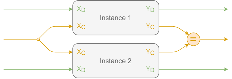
Figure 2: UPEC-DIT Computational Model

Fig. 2 shows the abstract computational model for the proposed methodology. Like previous UPEC approaches, UPEC-DIT is based on a 2-safety computational model. In our model, inputs and outputs of the design are partitioned into control and data signals. This is a manual step that, in most cases, is straightforward and can be done by consulting the design specification. Generally speaking, any confidential information passing through the system must be marked as data. After the partitioning, the generation of the 2-safety model can be fully automated. The control inputs $X_{C}$ take arbitrary but equal values, whereas the data inputs $X_{D}$ remain unconstrained. According to Def. 1, our goal is to prove that for any sequence of inputs, the control outputs $Y_{C}$ never diverge from their respective counterparts in the other instance.

IV-C The UPEC-DIT Property

Fig. 3 shows our IPC property template to formally verify the data-obliviousness of the design.

UPEC-DIT-Step($Z_{C},Y_{C},\phi,B_{\phi}$):
assume:
	at $t$:	Control_State_Equivalence($Z_{C}$);
	at $t$:	Invariants($B_{\phi}$);
	during $t$..$t$+$1$:	Input_Constraints($\phi$);
prove:
	at $t$+$1$:	Control_State_Equivalence($Z_{C}$);
	at $t$+$1$:	Invariants($B_{\phi}$);
	during $t$..$t$+$1$:	Control_Output_Equivalence($Y_{C}$);

Figure 3: Interval property template for UPEC-DIT

It expresses our abstract definitions introduced in Sec. III by standard property languages such as SVA. We iteratively refine this property with respect to $Z_{C}$, $\phi$ and $B_{\phi}$ during the execution of the UPEC-DIT algorithm. We now describe the individual components of the property, expressed as macros or functions, in more detail:

• Control_State_Equivalence() constrains the state holding signals related to control ($Z_{C}$) to be equal in both instances of the computational model. At the start of the algorithm, we set $Z_{C}=Z$, before iteratively refining this partitioning. We elaborate on how this is done in Sec. IV-D.

• Input_Constraints() exclude unwanted behavior to achieve input-constrained data-obliviousness (Def. 3). For systems specifically designed to be data-oblivious, such constraints might not be required. An example for this macro would be ”no new (data-dependent) division issued to the processor pipeline”.

• Invariants() are used to constrain the state space to exclude unreachable scenarios. These invariants are iteratively deduced during the main algorithm (Sec. IV-D). All invariants used to strengthen our properties are proven inductively on the fly, along with data-obliviousness, which is why the macro Invariants() is included also in the property commitment.

• Control_Output_Equivalence() is our main proof target and expresses that the outputs marked as control must never diverge.

It is important to note that the control inputs are already constrained in the computational model itself (cf. Fig. 2), and, therefore, are not specified in the property.

IV-D The UPEC-DIT Algorithm

Algorithm 1 The UPEC-DIT Algorithm

1:procedure UPEC-DIT

2:     $Z_{C}\leftarrow Z$

3:     $\phi,B_{\phi}\leftarrow\emptyset$

4:     CEX $\leftarrow$ IPC(UPEC-DIT-Step($Z_{C},Y_{C},\phi,B_{\phi}$))

5:     while CEX $\neq\{\}$ do

6:         if $Y_{C1}\neq Y_{C2}\in$ CEX then

7:              return CEX          

8:         for each $z\in Z_{C}:z_{1}\neq z_{2}\in$ CEX do

9:              if $z$ is $Data$ then

10:                  $Z_{C}=Z_{C}\backslash\{z\}$

11:              else if Invalid CEX then

12:                  Update($\phi,B_{\phi}$)

13:                  $Z_{C}\leftarrow Z$

14:                  break

15:              else

16:                  return CEX                        

17:         CEX $\leftarrow$ IPC(UPEC-DIT-Step($Z_{C},Y_{C},\phi,B_{\phi}$))      

18:     return hold

The basic idea of the UPEC-DIT algorithm is to use the counterexamples of the formal tool to iteratively refine the set of all states $Z$ into control and data subsets $Z_{C}$ and $Z_{D}$, respectively. Leveraging this partitioning of internal signals results in an inductive proof over only a single clock cycle, which scales even for very large designs.

Alg. 1 shows the algorithm in pseudocode. We begin by initializing the set of control states $Z_{C}$ with the set of all state signals $Z$ in Line 2. In the beginning, the set of input constraints $\phi$ and invariants $B_{\phi}$ is empty. We then call the formal property checker in Line 4 using the property in Fig. 3. In almost all cases, this will produce a counterexample CEX which shows a first propagation of data.

We then continuously investigate the returned counterexamples to decide on how to proceed: If a discrepancy has traveled to a control output (Line 6), we detected a data-dependent timing and return the respective counterexample. If a propagation to one or multiple internal signals has occurred (Line 8), the verification engineer has to decide if this information flow was valid or not. Whenever a propagation to a data signal, e.g., a pipeline buffer, is detected, we generalize the proof by removing this variable from the set of control signals (Line 10). In the case that the propagation hit a signal considered control, e.g., pipeline stalls or valid signals, the algorithm concludes and returns the counterexample (Line 16).

In some cases, the counterexamples may show behavior that is either unreachable or invalid in the given application scenario. An example for an invalid behavior could be the exclusion of certain instruction types for which data-obliviousness is not required, e.g., branches. To handle these cases, invariants or input constraints must be added to restrict the set of considered states (Line 12). Afterwards, we also reset the set of control signals $Z_{C}$. This is required for correctness, as an added input constraint might also make some previously considered propagation impossible. In our experiments, however, resetting $Z_{C}$ did not occur often and thus did not cause significant overhead. After every discrepancy in the counterexample has been investigated, we rerun the proof with the new assumptions (Line 17). This is continued until the proof holds and no new counterexample can be found by the formal property checker. In this case, the algorithm terminates. We continue by verifying the induction base, i.e., we check, as described in the following subsection, that our initial assumptions hold after a system reset.

It is important to note that the proposed methodology is conservative in the sense that if a control-related signal from $Z$ is mistakenly declared as data (Line 9), it will not result in a false security proof. In this case, the algorithm will continue until the propagation eventually reaches a control output $Y_{C}$ and returns the corresponding counterexample. The main purpose of the individual partitioning of the state set signals is to detect and stop such propagation as early as possible.

IV-E Induction Base

By successfully proving the inductive property (Fig. 3), we show that our 2-safety model never diverges in its control behavior during operation. For completing our proof of data-obliviousness, we also have to verify that the assumptions and invariants made in this inductive proof are correct. Therefore, the last step of the methodology is to prove the induction base, i.e., that the system starts in a data-oblivious state.

UPEC-DIT-Base($Z_{C},Y_{C},\phi,B_{\phi}$):
assume:
	during $t$-$k$..$t$-$1$:	Reset_Sequence();
	during $t$-$k$..$t$:	Input_Constraints($\phi$);
prove:
	at $t$:	Control_State_Equivalence($Z_{C}$);
	at $t$:	Invariants($B_{\phi}$);
	at $t$:	Control_Output_Equivalence($Y_{C}$);

Figure 4: Interval property template for UPEC-DIT Induction Base

Fig. 4 shows our IPC property template for the induction base. We want to show that the reachability assertions $B_{\phi}$ we introduced during the iterative algorithm include the reset state of the system, which means that they are indeed invariants according to Def. 4. Furthermore, we want to prove that the system is properly initialized regarding its control behavior. In essence, Control_State_Equivalence() ensures that all control state signals $Z_{C}$ are initialized. If this commitment fails, then the system could behave differently after a reset, which could hint to a functional bug. Lastly, by assuming Control_Output_Equivalence(), we verify that there is no combinatorial path from a data input $X_{D}$ to a control output $Y_{C}$.

When both the base and step property hold, we have exhaustively verified that our design operates data-obliviously, either in the strong sense of Def. 1, or for a subset of its total behavior in the weakened sense of Def. 3. This represents an unbounded formal proof that, due to its inductive nature, can scale to very large designs.

V Optimizations

The methodology described Sec. IV verifies data oblivious-behavior at the microarchitectural level exhaustively. In practice, it may not always be necessary to be exhaustive and an efficient bug-hunting may suffice for the intended application of some designs. In addition, the low complexity of certain designs allows for exhaustive verification of data-obliviousness at the I/O interface level, without the need for invariants and constraints on the internal behavior of the design. To this end, we now discuss some enhancements and trade-off techniques that may be useful for applying UPEC-DIT in practice.

V-A Unrolled Proofs

The methodology presented in Sec. IV uses an inductive proof with a single-cycle property to avoid complexity issues. In this approach, the set of all possible data propagation paths is over-approximated in the symbolic initial state by leaving the values of internal data signals unconstrained. While this over-approximation leads to a very low proof complexity, it implies the need to deal with the possibility of spurious counterexamples. Writing invariants can overcome this problem, but in some cases it is affordable to simply increase the computational effort to avoid these problems. If the complexity of the system allows for a sufficient number of unrollings in our computational model, considering the full propagation path starting from any data input to any control output can significantly reduce the number of false counterexamples and thus the effort of writing invariants. This unrolled approach represents the original UPEC-DIT methodology, as described in [17].

UPEC-DIT-Unrolled-IO($Z,Y_{C},\phi$):
assume:
	at $t$:	State_Equivalence($Z$);
	at $t$:	Input_Constraints($\phi$);
prove:
	during $t$..$t$+$k$:	Control_Output_Equivalence($Y_{C}$);

Figure 5: Unrolled UPEC-DIT property only considering I/O-behavior

The idea of unrolled proofs is shown in Fig. 5 and is a straightforward implementation of Def. 1. In this property, all state signals $Z$ are initialized to equal but arbitrary values between the two instances. This is denoted by the State_Equivalence() macro. We then prove that for a maximum latency $k$, the two instances maintain equal control outputs $Y_{C}$. We choose $k$ to be greater or equal to the length of the longest HW operation in the design. If this property fails, it means that the difference in $Y_{C}$ must originate from the data inputs $X_{D}$, since this is the only source of discrepancy between the two instances. In this case, the property checker returns a counterexample which guides the verification to the root cause by highlighting the deviating values.

The great advantage of this variant of UPEC-DIT is that it does not require an iterative partitioning of internal state signals $Z$. Therefore, the only manual steps are partitioning the system interface and choosing a maximum latency $k$. Everything else can be automated. For many low-complexity designs, such as functional units or accelerators, this approach can provide exhaustive proofs. It can also serve as a quick initial test for larger systems, as most timing channels become visible after only a few cycles. Unfortunately, this approach can run into scalability problems because the full propagation paths from input to output can be too long in more complex systems such as processor cores.

UPEC-DIT-Unrolled($Z,Z_{C},Y_{C},\phi$):
assume:
	at $t$:	State_Equivalence($Z$);
	at $t$:	Input_Constraints($\phi$);
prove:
	during $t$..$t$+$k$:	Control_State_Equivalence($Z_{C}$);
	during $t$..$t$+$k$:	Control_Output_Equivalence($Y_{C}$);

Figure 6: Unrolled UPEC-DIT property with internal state signals

A trade-off between computational complexity and a decreased number of false counterexamples is presented in Fig. 6. This variant of UPEC-DIT also starts by initializing all state signals $Z$ to equal but arbitrary values, and thus considers propagation paths starting from the data inputs. In this case however, we perform a partitioning of $Z$ into $Z_{C}$ and $Z_{D}$ based on Alg. 1. Having an internal representation of the control-flow allows for a much earlier detection of data-dependent side-effects. Furthermore, isolating the source of the discrepancy to the input makes the returned counterexamples more intuitive and less likely to be spurious.

Unfortunately, this approach does not scale well for complex systems beyond a few clock cycles. Nonetheless, this unrolled method can serve as a basis for the inductive proof, since the deduced partitioning of $Z$ is the same for both variants. Therefore, it often makes sense to start with the unrolled approach and set $k=1$. The verification engineer can then iteratively increase $k$ until no new counterexamples appear or the computational cost becomes prohibitive. Then the transition to the inductive method is made by initializing $Z_{C}$ in Line 2 of Alg. 1 with the remaining control state signals. In our experience, starting with an unrolled model makes the counterexamples more intuitive because it shows longer propagation paths starting from the inputs. This can be especially helpful early in the methodology, when the verification engineer has little to no knowledge or intuition about the design under verification. We have omitted the invariants in Fig. 5 and Fig. 6 because they are usually very simple when all state signals $Z$ are initialized to equal values.

Finally, we would like to point out that the unrolled property (Fig. 6) can also be used in an effective bug hunting approach that trades formal/exhaustive coverage for efficiency. Instead of executing the full iterative algorithm that refines the set of state signals systematically (required for formal exhaustiveness), we can specify Control_State_Equivalence() using a set of state signals identified as control manually, and run the proof. The verification engineer determines the control variables based on knowledge and experience. Obvious examples of control signals are stall variables in a processor pipeline. Empirical evidence from our experiments shows that almost all timing vulnerabilities manifest themselves in only a handful of control signals. While this short-cut over the formal algorithm bears a certain risk of missing corner-case behavior, it avoids the potentially laborious iterative procedure and produces high-quality results fast. It may be a viable option in certain practical scenarios.

V-B Black-Boxing

Black-boxing can significantly increase the scalability of the formal proof. Essentially, black-boxing excludes the functionality of certain components from the system, reducing the complexity of the computational model. When a module is black-boxed, its inputs become outputs of the system under verification. Likewise, any output of the module connected to the rest of the system is now considered as an open input, since the functionality of that component is no longer considered. In particular, for state-heavy submodules, such as caches, their black-boxing can greatly simplify the overall state space for the formal proof. Many commercial formal tools provide black-boxing as a fully automated, built-in feature.

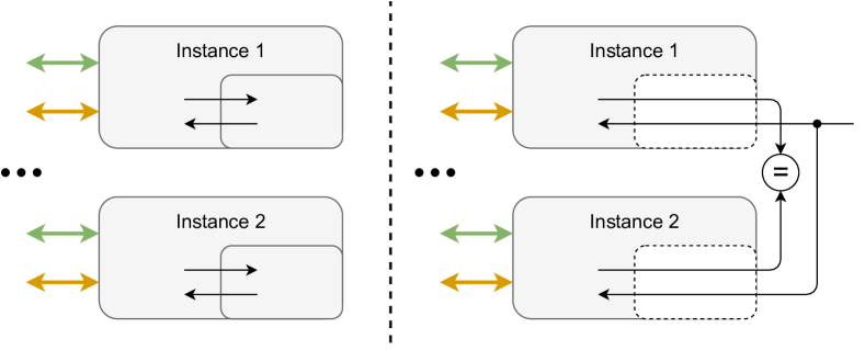
Figure 7: Computational Model before and after sound black-boxing

While black-boxing significantly reduces the overall complexity of the formal proof, it can lead to false counterexamples or even verification gaps in standard functional verification. Fortunately, the 2-safety computational model of UPEC-DIT allows for a sound black-boxing to ensure that no security violations are missed. We accomplish this by monitoring the interface of the black-boxed component, as shown in Fig. 7. By checking that the data traveling to the black-box is equal in both instances, UPEC-DIT detects any propagation involving a submodule that could result in a future data-dependent timing behavior. False counterexamples are prevented in our approach by constraining all the outputs of the black-boxed component to be equal between the two instances.

If a counterexample is produced that shows a difference at the black-box inputs, the verification engineer can decide to either undo the black-boxing or examine the module individually. The first option requires less effort but results in higher computational complexity, while the second option requires more manual effort but can lead to a better understanding of the system and simpler counterexamples. We will explore the second option further in the following subsection.

V-C Modularization

Setting up formal proofs from scratch for a very large system can be a difficult task. Therefore, it is often advisable to decompose the problem and to first look at individual components that are ”suspicious” or critical to security. Examples would be a cryptographic accelerator or, in the case of a processor, the various functional units of the pipeline.

Investigating an individual component results in a less complex computational model, simpler counterexamples, and helps to establish a better understanding of the system. We can utilize the same inductive approach as elaborated in Sec. IV or, if computational complexity permits, the unrolled approach described in Sec. V-A. If a counterexample is found for a single module, it is very likely that it also indicates a security threat to the entire system. If a component turns out to be data-oblivious, we can use this information to simplify our computational model of the system using black-boxing (Sec. V-B). For this purpose, we consider the control (data) inputs of the black-box as control (data) outputs of the system and the control (data) outputs of the black-box as control (data) inputs of the system. Therefore, we can skip the data propagation through the black box and use its data output as a new source of discrepancy. This allows us to systematically partition the formal proof in a divide-and-conquer fashion, making it scalable even for very large systems.

V-D Proof Parallelization

UPEC-DIT-Step-z($z,Z_{C},Y_{C},\phi,B_{\phi}$):
assume:
	at $t$:	Control_State_Equivalence($Z_{C}$);
	at $t$:	Invariants($B_{\phi}$);
	during $t$..$t$+$1$:	Input_Constraints($\phi$);
prove:
	at $t+1$:	Equivalence($z$);
	at $t+1$:	Invariants($B_{\phi}$);
	during $t$..$t$+$1$:	Control_Output_Equivalence($Y_{C}$);

Figure 8: Parameterized UPEC-DIT-Step Property

Splitting and parallelizing the proof is another optimization of the algorithm that can be fully automated. The fundamental idea is that each propagation candidate can be checked independently. For this purpose, we modify our property to take a parameter $z\in Z$, as shown in Fig. 8. The Equivalence(z) macro in the prove part of our property checks that $z$ maintains equality between the two instances of the computational model.

Instead of proving all possible propagation paths at once in Alg. 1, we now generate and prove an individual property for each $z\in Z_{C}$ (Line 4 and Line 17). Each individual property can have a significantly reduced runtime compared to the global property, especially when considering an unrolled proof (Sec. V-A). If sufficient computing resources are available to run multiple properties in parallel, this step can reduce the overall runtime of the methodology.

The same idea of splitting the proof can also be applied to the control outputs. However, since their number is usually much smaller than the number of state signals, this does not significantly improve the overall runtime in most cases.

V-E Cone-of-Influence Reduction

The UPEC-DIT property in Fig. 3 checks all internal control signals $Z_{C}$ for a possible data propagation. However, data can only propagate into state signals that are in the sequential fan-out of already deviating signals. So instead of checking for Control_State_Equivalence(), we can check for the equivalence of all state signals that are in the fan-out of $I\cup Z\backslash Z_{C}$. Since this step is based solely on structural information, it can be fully automated with the help of dedicated tools.

This cone-of-influence reduction can also be used to further improve proof parallelization (Sec. V-D). By reducing the number of signals considered, the total number of parallelized properties is also reduced.

VI Experiments

VI-A Example: SHA512 Core

We begin our practical evaluation with a practical example demonstrating the proposed methodology in detail, namely an open-source implementation of a cryptographic accelerator implementing the SHA512 algorithm [36]. A timing channel in such a core can create severe security flaws, as it can significantly reduce the strength of the underlying encryption. Therefore, we want to exhaustively verify that no data-dependent timing behavior exists in this accelerator.

We begin by looking at the interface of the module along with its specification. The core implements 5 inputs (clk_i, rst_i, text_i, cmd_i and cmd_w_i) and 2 outputs (text_o and cmd_o). After referring to the documentation, we mark the clock, reset and handshaking signals (cmd) as control, while the plain and cipher text ports are marked as data. Our goal is to prove that the accelerator is data-oblivious according to Def. 1, i.e., the data input text_i has no influence on the control output cmd_o.

The next step is to generate our 2-safety computational model (Fig. 2), in which the control inputs are constrained to be equal, while the data input remains unconstrained. We also generate a macro for State_Equivalence() that constrains each of the 37 state-holding signals (2162 flip-flops) to equal values between the two instances at the start of our proof. Given the I/O partitioning, both steps can be fully automated with dedicated tool support.

We can now choose to formulate either a single-cycle or an unrolled proof. For an exhaustive proof over multiple clock cycles, we have to unroll the model to its sequential depth, as elaborated in Sec. V-A. According to the specification, one encryption operation has a latency of 97 clock cycles. Since the complexity of this module is rather low, it is still possible to unroll the formal proof for several hundred cycles. For more complex accelerators, this is usually not feasible.

Therefore, to show the effectiveness of the UPEC-DIT methodology, we decide to iteratively create an inductive single-cycle proof using Alg. 1. We begin by setting up the UPEC-DIT-Step property (Fig. 3 in Sec. IV-C) in such a way that Control_State_Equality() considers all 37 state holding signals $Z$ of the design and Control_Output_Equality() ensures the equality of cmd_o. After running the verification tool, we receive a first counterexample showing a discrepancy propagation to two internal pipeline buffers (W3 and Wt). Since these are used to store intermediate results of the encryption, we classify them as data, exclude them from the macro and rerun the proof.

After several iterations of checking the UPEC-DIT-Step property, a fixed point is reached with only 5 out of 37 signals left in $Z_{C}$: busy, cmd, read_counter, round and Kt. All other signals only store intermediate results and were therefore marked as data and removed from the proof. This means that even though a vast majority of the design can be in an arbitrary state, the timing behavior only depends on certain control registers inside the design.

The last step is to verify the induction base with the UPEC-DIT-Base property (Fig. 4 in Sec. IV-E), which also holds. Hence, we successfully showed that the SHA core operates timing-independent w.r.t. its input data. With some experience, the entire proof procedure can be completed in less than an hour.

VI-B Functional Units and Accelerators

TABLE I: Results for functional units

Design	DIT	#States	Time	Mem
BasicRSA	✗	532	<1s	589 MB
SHA1	✓	911	<1s	306 MB
SHA256	✓	1103	<1s	296 MB
SHA512	✓	2162	<1s	329 MB
AES1	✓	2472	4s	994 MB
AES2	✓	554	<1s	819 MB
FWRISCV MDS-Unit	(!)	331	<1s	596 MB
ZipCPU Div-Unit	✗	142	11s	1347 MB
CVA6 Div-Unit	✗	209	<1s	580 MB

For each entry, we list whether or not the design has data-independent timing (DIT), number of state bits, total proof time and peak memory usage.

Tab. I shows the results for several functional units and accelerators. All of these experiments were conducted using the unrolled approach as elaborated in Sec. V-A.

The first design, BasicRSA, was taken from OpenCores [37] and implements an RSA encryption. Using the UPEC-DIT methodology, we detected a timing side channel in the design. The FU computes the modular exponentiation needed for the encryption algorithm in a square-and-multiply fashion. While this approach is very efficient, it makes the encryption time directly dependent on the size of the secret key. We also took a separate look at the submodule that is responsible for performing the modular multiplication. This FU also turned out not to be data-oblivious, since its timing depends on the size of the multiplier.

SHA1, SHA256 and SHA512 [36] implement different variants of the Secure Hash Algorithm. AES1 and AES2 are different implementations of the Advanced Encryption Standard. All of these accelerators were proven by UPEC-DIT to have data-independent timing.

The Multiplication-Division-Shifting-Unit is part of the Featherweight RISC-V [38] project. Its goal is to build a resource-efficient implementation for FPGAs. All of its operations take multiple clock cycles, shifting only one bit in each cycle. In this FU, multiplication and division were proven to execute data-independently, requiring 33 cycles to complete. However, UPEC-DIT produced a counterexample for shift operations, as the timing is directly dependent on the shift amount. To perform a shift by N bits, the module sets its internal counter value to N which causes the operation to take N+1 cycles in total. This can be dangerous because shift operations are considered data-independent in almost all applications.

The last two designs are serial division units taken from the ZipCPU [39] and CVA6 [40] open-source projects. Both FUs showed strong dependencies of their timing w.r.t. their operands. ZipCPU implements an early termination when dividing by zero. Also, if the signs of the operands are different, the division takes an additional cycle. The CVA6 FU implements certain optimizations for HW division which entail that the division time is determined by the difference in leading zeros of the operands. This creates a data dependency.

In all case studies, UPEC-DIT was applied without a priori knowledge of the designs. It systematically guided the user to the points of interest. Even though the designs have operations taking up to 192 cycles, proof time and memory requirements remained insignificant. Furthermore, operations like multiplication, which are usually a bottleneck for formal tools, did not cause any complexity issues. This is by merit of the proposed 2-instance computational model which abstracts from functional signal valuations and only considers the difference between the two instances.

VI-C In-Order Processor Cores

TABLE II: Results for in-order processors

	FW	IBEX	(+DIT)	SCARV	CVA6
I-Type	✓	✓	✓	✓	✓
R-Type	✓/✗	✓/✓	✓/✓	✓/✓	✓/✓
Mult	✓/✓	✓/✗	✓/✓	✓/✓	✓/✓
Div	✓/✓	✓/✗	✓/✓	✓/✓	✗/✗
Load	(!)	(!)	(!)	✗	✗
Store	(!)/✓	(!)/✓	(!)/✓	✗/✗	✗/✓
Jump	(!)	✓	✓	(!)	✗
Branch	✗/✗	✗/✗	✓/✓	✗/✗	✗/✗
#States	3086	1019	1021	2334	682849
AT	0:03	2:06	4:24	3:27	1:35:41
WCT	0:04	5:11	6:40	8:02	3:06:43
Mem	1.7	4.5	4.3	2.1	11.9

In each experiment (separate proof), UPEC-DIT proved that the instruction class executes data-independently either always (✓), only under certain SW restrictions ((!)), or not at all, i.e, it depends on its operands (✗). Multi-operand instructions denote rs1/rs2 separately, as they can have different impact on timing. We also report the number of state bits in the original design, the average time (AT) and worst-case time (WCT) of a single proof (HH:MM:SS) as well as the peak memory requirements (GB).

We investigated four different open-source in-order RISC-V processors from low to medium complexity, as shown in Tab. II. The Ibex processor is listed twice, as it comes with a data-independent timing (DIT) security feature, which we examined separately. All of these experiments were conducted using the unrolled approach as elaborated in Sec. V-A. The results for this approach show that time and memory requirements are still moderate, even in the case of a medium-sized processor.

The first design we investigated is the sequential Featherweight RISC-V [38] processor which aims at balancing performance with FPGA resource utilization. As our results show, most instructions execute independently of their input data. However, there was one big exception, namely, R-Type shift instructions. For area efficiency, the implementation shares a single shifting unit for multiplication, division and shifting. The shifting unit can only shift one bit in each cycle (cf. VI-B), which results in data-dependent timing depending on the shift amount (rs2). We singled out the shift instructions in a separate proof and showed that other R-Type instructions like addition do, in fact, preserve data-independent timing. Note that I-Type shift instructions also execute with dependence on the shift amount. The shift amount, however, is specified in the (public) immediate field of the instruction. Consequently, since the program itself is viewed as public, I-Type shifting executes data-obliviously. Load, Store and Jump (JALR) can cause an exception in case of a misaligned address, while Branches incur a penalty if a branch is not taken.

The Ibex RISC-V Core [20] is an extensively verified, production-quality open-source 32-bit RISC-V CPU. It is maintained by the lowRISC not-for-profit company and deployed in the OpenTitan platform. It is highly configurable and comes with a variety of security features, including a data-independent timing (DIT) mode. When activating this mode during runtime, execution times of all instructions are supposed to be independent of input data. In our experiments, we apply UPEC-DIT for both inactive and active DIT mode and use the default ”small” configuration, with the ”slow” option for multiplication.

When the DIT mode is turned off, we found three cases of data-dependent execution time:

• Division and (slow) multiplication implement fast paths for certain scenarios.

• Taken branches cause a timing penalty, as the prefetch buffer has to be flushed.

• Misaligned loads and stores are split into two aligned memory accesses.

The first two issues are solved when DIT mode is active, as seen in Tab. II. All fast paths are deactivated and non-taken branches now introduce a delay to equal the timing of taken branches. However, the timing violation for misaligned memory accesses is not addressed.

When running Ibex in DIT mode, data-oblivious memory accesses require special measures, such as the integration of the core with a data-oblivious memory sub-system. For example, an oblivious RAM controller [41] makes any memory access pattern computationally indistinguishable from any other access pattern of the same length. However, our experiments with UPEC-DIT reveal that even with such strong countermeasures in place, Ibex still suffers from a side channel in the case of memory accesses that are misaligned. This is because the core creates a different number of memory requests for aligned and misaligned accesses. We reported this issue to the lowRISC team and suggested to disable the misaligned access feature for DIT mode. With this fix, the HW would remain secure even in case that a faulty/malicious SW introduces a misaligned access. The lowRISC team refined the documentation and will consider the proposed fix for future updates of the core.

The SCARV [42] is a 5-stage single-issue in-order CPU core, implementing the RISC-V RV32IMC instruction sets. We prove that most instructions do not leak information through timing by running UPEC-DIT on the core. Taken branches, however, use additional cycles due to a pipeline flush. Memory accesses can cause exceptions if they are misaligned. Furthermore, any loads and stores to a specific address region are interpreted as memory-mapped I/O accesses which do not issue a memory request. This can be used to set a SW interrupt timer depending on the store value, thus creating data-dependent timing. CVA6 [40], also known as Ariane, is a 6-stage, single-issue 64-bit CPU. Having almost 700 k state bits, the design itself already pushes the limits of formal property checkers. To make things worse, a straightforward 2-safety circuit model would have twice as many state bits. Fortunately, UPEC-DIT allows for sound black-boxing to cope with complexity issues (cf. Sec. V-B).

Black-boxing reduces the computational model to 24 k state bits. For load and store instructions, a couple of exception scenarios showed up: Access faults (PMP), misaligned addresses or page faults. Besides a data-dependent division and timing variations by mispredicted branches UPEC-DIT also found an interesting case in which a load can be delayed. In order to prevent RAW hazards, whenever a load is issued, the store buffer is checked for any outstanding stores to the same offset. If any exist, the load is, conservatively, stalled until the stores have been committed. However, this can cause a timing delay in case of a matching offset, even if both memory accesses go to different addresses.

VI-D UPEC-DIT with Inductive Proofs

In this subsection, we extend our experiments to the BOOM [21], a superscalar RISC-V processor with FP support, a deep 10-stage pipeline and out-of-order execution.

In a first attempt, the same unrolled approach (cf. Sec. V-A), as above for in-order processors, was applied to BOOM, and UPEC-DIT was able to prove the data-obliviousness of basic arithmetic instructions and multiplication. However, the high design complexity caused by the deep pipeline pushed the formal tools to their limits, with some proof times exceeding 20 hours. Fortunately, with a few design-specific adjustments, it was still possible to formally verify the absence of any data-dependent side-effects. These optimizations included splitting the verification into individual proofs for the integer and FP pipelines, since these are implemented as separate modules in BOOM. To do this, we constrained the outputs of the FP register file to be equal for the integer pipeline verification and vice versa. After unrolling for 7 clock cycles, no new propagation was detected in either pipeline. Furthermore, a sound black-boxing (cf. Sec. V-B) of complex components, such as the re-order buffer (ROB) and caches, was performed, significantly reducing the complexity of the computational model: While a single instance of BOOM has more than 500k state bits, our final 2-safety model contained only about 47k state bits.

Black-boxing the ROB not only reduces the size of the computational model, but also drastically reduces the complexity of spurious counterexamples caused by the symbolic initial state. During normal operation of an out-of-order processor, the ROB reflects the control state of the entire system. Assuming an arbitrary initial state can therefore lead to many false counterexamples where the ROB in no way reflects the state of the computational pipeline. Fortunately however, the actual state of the ROB is of no concern to UPEC-DIT, as long as instructions commit to it equally between the two instances. We can therefore create a black-box and consider its inputs in our proof statement.

Nevertheless, the long proof times caused by the high complexity made us rethink the approach. Thus, we extended the methodology and developed the inductive proof, as presented in Sec. IV, which spans over only a single clock cycle. Eliminating the need to unroll the circuit drastically reduced the complexity of the computational model, diminishing individual proof times from over 20 hours to just a few seconds. In this transition, we also found that in most cases, data can only affect the control flow through a few specific channels. This insight made it easier to find meaningful invariants and constraints that restrict the over-approximated state space in order to avoid false counterexamples.

TABLE III: Results for inductive proofs

Design	#States	#Data Signals	#BB	Time	Mem.
BOOM (Int)	46958	31	4	5s	1.6GB
BOOM (FP)	46958	143	4	5s	2.0GB
CVA6	23484	22	7	58s	3.1GB

For each experiment, the table shows the size of the final computational model, the number of (unconstrained) data signals within per instance, the number of black-boxes per instance, and the time and memory consumption of the final inductive step proof.

Tab. III shows the results in terms of computational complexity for the inductive proofs. We also re-run our experiment on CVA6 [40] to illustrate the improvement in scalability compared to an unrolled proof. As shown in the table, proof time and memory usage are reduced significantly by eliminating the need to unroll the model. In CVA6, data propagates through 22 internal signals ($Z_{D}$), which can take arbitrary values in the final proof. By assuming the equality of two internal signals, we excluded division and control and status register (CSR) operations from consideration. Branches and Load/Store instructions were excluded by black-boxing the branch unit and the load-store unit (LSU).

The experiments in BOOM were split for the integer and FP pipelines. Within the integer pipeline, UPEC-DIT detected data propagation into 31 internal signals ($Z_{D}$). We excluded branches, division, and misaligned memory accesses after receiving counterexamples for each of these cases. Inside the FP pipeline, data is propagated into 143 internal data signals ($Z_{D}$). However, only counterexamples caused by FP division and square root had to be excluded from the proof with constraints.

For BOOM, our results show that branch, integer division, FP division, and square-root operations have data-dependent timing. We have not examined memory access instructions, as these are usually given special treatment in constant-time programming. The remaining integer arithmetic instructions (including multiplication) were formally proven to execute data-obliviously. An interesting case are FP arithmetic instructions: Although their timing is independent of their operands, they are not data-oblivious. UPEC-DIT revealed that these instructions can still leave a side effect in the form of an exception flag in the FP CSR named fcsr. This is in compliance with the ISA specification of RISC-V. However, in order to create a timing side channel, a victim program would have to explicitly load these registers. Therefore, these instructions could, in fact, be used securely for constant-time programming, if a suitable SW restriction was introduced.

VII Conclusion

In this paper, we proposed UPEC-DIT, a novel methodology for formally verifying data-independent execution in RTL designs. We proposed an approach based on an inductive property over a single clock cycle, which facilitates a verification methodology scalable even to complex out-of-order processors. We presented and discussed several techniques that can help the verification engineer simplify and accelerate the verification process. UPEC-DIT was evaluated against several open-source designs, ranging from small functional units to a complex out-of-order processor. While many of the implemented instructions execute as expected, UPEC-DIT uncovered some unexpected timing violations. Our future work will address the design of security-conscious hardware. We envision that UPEC-DIT, if integrated in standard design flows, can make significant contributions to restoring the trust in the hardware for confidential computing.

Lucas Deutschmann received the M.Sc. degree in Electrical and Computer Engineering from RPTU Kaiserslautern-Landau, Kaiserslautern, Germany, in 2019. He is currently pursuing a doctoral degree with Electronic Design Automation group at the same institution. His current research interests include formal verification, hardware security, side channel attacks and data-oblivious computing.

Johannes Müller received the Dipl.-Ing. degree in Electrical and Computer Engineering from RPTU Kaiserslautern-Landau, Kaiserslautern, Germany, in 2018. He is currently pursuing a doctoral degree with Electronic Design Automation group at the same institution. His current research interests include formal verification, access control in SoCs and microarchitectural timing side channels.

Mohammad Rahmani Fadiheh received the M.Sc. degree in Electrical and Computer Engineering from RPTU Kaiserslautern-Landau, Kaiserslautern, Germany, in 2017, and the Dr.-Ing. degree in Electrical Engineering from the same institution in 2022. He is currently working as a postdoctoral researcher in the Department of Electrical Engineering at Stanford University, Stanford, USA. His current research interests include formal verification, hardware security, side channel attacks and secure hardware design.

Dominik Stoffel received the Dipl.-Ing. degree from the University of Karlsruhe, Karlsruhe, Germany, in 1992, and the Dr. phil. nat degree from Johann-Wolfgang Goethe Universität, Frankfurt, Germany, in 1999. He has held positions with Mercedes-Benz, Stuttgart, Germany, and the Max-Planck Fault-Tolerant Computing Group, Potsdam, Germany. Since 2001, he has been a Research Scientist and a Professor with the Electronic Design Automation group, RPTU Kaiserslautern-Landau, Kaiserslautern, Germany. His current research interests include design and verification methodologies for Systems-on-Chip.

Wolfgang Kunz received the Dipl.-Ing. degree in Electrical Engineering from University of Karlsruhe in 1989, the Dr.-Ing. degree in Electrical Engineering from University of Hannover in 1992 and the Habilitation degree from University of Potsdam (Max Planck Society, Fault-Tolerant Computing Group) in 1996. Since 2001 he is a professor at the Department of Electrical and Computer Engineering at RPTU Kaiserslautern-Landau, Kaiserslautern, Germany. Wolfgang Kunz conducts research in the area of System-on-Chip design and verification. His current research interests include verification-driven design methodologies for hardware and firmware, safety analysis and hardware security.

References

- [1] B. Coppens, I. Verbauwhede, K. De Bosschere, and B. De Sutter, “Practical mitigations for timing-based side-channel attacks on modern x86 processors,” in 2009 30th IEEE symposium on security and privacy. IEEE, 2009, pp. 45–60.
- [2] S. Cauligi, C. Disselkoen, K. v. Gleissenthall, D. Tullsen, D. Stefan, T. Rezk, and G. Barthe, “Constant-time foundations for the new spectre era,” in Proceedings of the 41st ACM SIGPLAN Conference on Programming Language Design and Implementation, 2020, pp. 913–926.
- [3] “BearSSL,” https://www.bearssl.org/, 2018.
- [4] “A beginner’s guide to constant-time cryptography,” https://www.chosenplaintext.ca/articles/beginners-guide-constant-time-cryptography.html, 2023.
- [5] M. Andrysco, D. Kohlbrenner, K. Mowery, R. Jhala, S. Lerner, and H. Shacham, “On subnormal floating point and abnormal timing,” in 2015 IEEE Symposium on Security and Privacy, 2015, pp. 623–639.
- [6] L. C. Meier, S. Colombo, M. Thiercelin, and B. Ford, “Constant-time arithmetic for safer cryptography,” Cryptology ePrint Archive, Paper 2021/1121, 2021, https://eprint.iacr.org/2021/1121. [Online]. Available: https://eprint.iacr.org/2021/1121
- [7] S. Cauligi, G. Soeller, F. Brown, B. Johannesmeyer, Y. Huang, R. Jhala, and D. Stefan, “FaCT: A flexible, constant-time programming language,” in 2017 IEEE Cybersecurity Development (SecDev). IEEE, 2017, pp. 69–76.
- [8] J. B. Almeida, M. Barbosa, G. Barthe, F. Dupressoir, and M. Emmi, “Verifying constant-time implementations,” in 25th USENIX Security Symposium (USENIX Security 16), 2016, pp. 53–70.
- [9] B. Rodrigues, F. M. Quintão Pereira, and D. F. Aranha, “Sparse representation of implicit flows with applications to side-channel detection,” in Proceedings of the 25th International Conference on Compiler Construction, ser. CC 2016. New York, NY, USA: Association for Computing Machinery, 2016, p. 110–120. [Online]. Available: https://doi.org/10.1145/2892208.2892230
- [10] O. Reparaz, J. Balasch, and I. Verbauwhede, “Dude, is my code constant time?” in Proceedings of the Conference on Design, Automation and Test in Europe, ser. DATE ’17. Leuven, BEL: European Design and Automation Association, 2017, p. 1701–1706.
- [11] P. Chakraborty, J. Cruz, C. Posada, S. Ray, and S. Bhunia, “HASTE: Software security analysis for timing attacks on clear hardware assumption,” IEEE Embedded Systems Letters, vol. 14, no. 2, pp. 71–74, 2022.
- [12] M. Andrysco, A. Nötzli, F. Brown, R. Jhala, and D. Stefan, “Towards verified, constant-time floating point operations,” in Proceedings of the 2018 ACM SIGSAC Conference on Computer and Communications Security, ser. CCS ’18. New York, NY, USA: Association for Computing Machinery, 2018, p. 1369–1382. [Online]. Available: https://doi.org/10.1145/3243734.3243766
- [13] G. Barthe, S. Blazy, B. Grégoire, R. Hutin, V. Laporte, D. Pichardie, and A. Trieu, “Formal verification of a constant-time preserving C compiler,” Proc. ACM Program. Lang., vol. 4, no. POPL, dec 2019. [Online]. Available: https://doi.org/10.1145/3371075
- [14] A. Ardeshiricham, W. Hu, and R. Kastner, “Clepsydra: Modeling timing flows in hardware designs,” in IEEE/ACM International Conference on Computer-Aided Design (ICCAD). IEEE, 2017, pp. 147–154.
- [15] K. v. Gleissenthall, R. G. Kıcı, D. Stefan, and R. Jhala, “IODINE: Verifying constant-time execution of hardware,” in 28th USENIX Security Symposium (USENIX Security 19), 2019, pp. 1411–1428.
- [16] K. v. Gleissenthall, R. G. Kıcı, D. Stefan, and R. Jhala, “Solver-aided constant-time hardware verification,” in Proceedings of the 2021 ACM SIGSAC Conference on Computer and Communications Security, ser. CCS ’21. New York, NY, USA: Association for Computing Machinery, 2021, p. 429–444. [Online]. Available: https://doi.org/10.1145/3460120.3484810
- [17] L. Deutschmann, J. Müller, M. R. Fadiheh, D. Stoffel, and W. Kunz, “Towards a formally verified hardware root-of-trust for data-oblivious computing,” in Proceedings of the 59th ACM/IEEE Design Automation Conference, ser. DAC’22. New York, NY, USA: Association for Computing Machinery, 2022, p. 727–732. [Online]. Available: https://doi.org/10.1145/3489517.3530981
- [18] J. R. S. Vicarte, P. Shome, N. Nayak, C. Trippel, A. Morrison, D. Kohlbrenner, and C. W. Fletcher, “Opening Pandora’s box: A systematic study of new ways microarchitecture can leak private data,” in ACM/IEEE 48th Annual International Symposium on Computer Architecture (ISCA), 2021.
- [19] J. S. Vicarte, M. Flanders, R. Paccagnella, G. Garrett-Grossman, A. Morrison, C. Fletcher, and D. Kohlbrenner, “Augury: Using data memory-dependent prefetchers to leak data at rest,” in 2022 IEEE Symposium on Security and Privacy (SP). IEEE Computer Society, 2022, pp. 1518–1518.
- [20] “Ibex RISC-V core,” https://github.com/lowRISC/ibex, 2021.
- [21] J. Zhao, B. Korpan, A. Gonzalez, and K. Asanović, “SonicBOOM: The 3rd generation berkeley out-of-order machine,” in Fourth Workshop on Computer Architecture Research with RISC-V, May 2020.
- [22] W. Hu, A. Ardeshiricham, and R. Kastner, “Hardware information flow tracking,” ACM Comput. Surv., vol. 54, no. 4, may 2021. [Online]. Available: https://doi.org/10.1145/3447867
- [23] Z. Wang, G. Mohr, K. von Gleissenthall, J. Reineke, and M. Guarnieri, “Specification and verification of side-channel security for open-source processors via leakage contracts,” arXiv preprint arXiv:2305.06979, 2023.
- [24] Y. Hsiao, D. P. Mulligan, N. Nikoleris, G. Petri, and C. Trippel, “Scalable assurance via verifiable hardware-software contracts,” in First Workshop on Open-Source Computer Architecture Research (OSCAR), 2022.
- [25] ——, “Synthesizing formal models of hardware from RTL for efficient verification of memory model implementations,” in MICRO-54: 54th Annual IEEE/ACM International Symposium on Microarchitecture, ser. MICRO’21. New York, NY, USA: Association for Computing Machinery, 2021, p. 679–694. [Online]. Available: https://doi.org/10.1145/3466752.3480087
- [26] “Data operand independent timing instruction set architecture (ISA) guidance,” https://www.intel.com/content/www/us/en/developer/articles/technical/software-security-guidance/best-practices/data-operand-independent-timing-isa-guidance.html, 2023.
- [27] “Arm Armv8-A architecture registers,” https://developer.arm.com/documentation/ddi0595/2021-06/AArch64-Registers/DIT--Data-Independent-Timing, 2021.
- [28] A. Waterman, Y. Lee, D. A. Patterson, and K. Asanović, “The RISC-V instruction set manual. volume 1: User-level ISA, version 2.0,” California Univ Berkeley Dept of Electrical Engineering and Computer Sciences, Tech. Rep., 2014.
- [29] “RISC-V cryptography extension,” https://github.com/riscv/riscv-crypto, 2023.
- [30] J. Yu, L. Hsiung, M. El Hajj, and C. W. Fletcher, “Data oblivious ISA extensions for side channel-resistant and high performance computing.” in The Network and Distributed System Security Symposium (NDSS), 2019.
- [31] ——, “Creating foundations for secure microarchitectures with data-oblivious ISA extensions,” IEEE Micro, vol. 40, no. 3, pp. 99–107, 2020.
- [32] M. D. Nguyen, M. Thalmaier, M. Wedler, J. Bormann, D. Stoffel, and W. Kunz, “Unbounded protocol compliance verification using interval property checking with invariants,” IEEE Transactions on Computer-Aided Design, vol. 27, no. 11, pp. 2068–2082, November 2008.
- [33] J. Urdahl, D. Stoffel, and W. Kunz, “Path predicate abstraction for sound system-level models of RT-level circuit designs,” IEEE Trans. on Comp.-Aided Design of Integrated Circuits & Systems, vol. 33, no. 2, pp. 291–304, Feb. 2014.
- [34] J. Müller, M. R. Fadiheh, A. L. D. Antón, T. Eisenbarth, D. Stoffel, and W. Kunz, “A formal approach to confidentiality verification in SoCs at the register transfer level,” in 58th ACM/IEEE Design Automation Conference, DAC 2021, San Francisco, CA, USA, December 5-9, 2021. IEEE, 2021, pp. 991–996.
- [35] M. R. Fadiheh, A. Wezel, J. Müller, J. Bormann, S. Ray, J. M. Fung, S. Mitra, D. Stoffel, and W. Kunz, “An exhaustive approach to detecting transient execution side channels in RTL designs of processors,” IEEE Transactions on Computers, vol. 72, no. 1, pp. 222–235, 2023.
- [36] “SHA cores,” https://opencores.org/projects/sha_core, 2018.
- [37] “Basic RSA encryption engine,” https://opencores.org/projects/basicrsa, 2018.
- [38] M. Ballance, “Featherweight RISC-V,” 2021. [Online]. Available: https://github.com/Featherweight-IP/fwrisc
- [39] “Zip CPU,” https://github.com/ZipCPU/zipcpu, 2021.
- [40] F. Zaruba and L. Benini, “The cost of application-class processing: Energy and performance analysis of a linux-ready 1.7-ghz 64-bit RISC-V core in 22-nm FDSOI technology,” IEEE Transactions on Very Large Scale Integration (VLSI) Systems, vol. 27, no. 11, pp. 2629–2640, Nov 2019.
- [41] C. W. Fletcher, L. Ren, A. Kwon, M. Van Dijk, E. Stefanov, D. Serpanos, and S. Devadas, “A low-latency, low-area hardware oblivious ram controller,” in 2015 IEEE 23rd Annual International Symposium on Field-Programmable Custom Computing Machines. IEEE, 2015, pp. 215–222.
- [42] “SCARV,” https://github.com/scarv/scarv-cpu, 2021.