The CARMENES search for exoplanets around M dwarfs

The hydrogen Paschen lines are known activity indicators, but studies of them in M dwarfs during quiescence are as rare as their reports in flare studies. This situation is mostly caused by a lack of observations, owing to their location in the near-infrared regime, which is covered by few high-resolution spectrographs. We study the Pa$\beta$ line, using a sample of 360 M dwarfs observed by the CARMENES spectrograph. Descending the spectral sequence of inactive M stars in quiescence, we find the Pa$\beta$ line to get shallower until about spectral type M3.5 V, after which a slight re-deepening is observed. Looking at the whole sample, for stars with H$\alpha$ in absorption, we find a loose anti-correlation between the (median) pseudo-equivalent widths (pEWs) of H$\alpha$ and Pa$\beta$ for stars of similar effective temperature. Looking instead at time series of individual stars, we often find correlation between pEW(H$\alpha$) and pEW(Pa$\beta$) for stars with H$\alpha$ in emission and an anti-correlation for stars with H$\alpha$ in absorption. Regarding flaring activity, we report the automatic detection of 35 Paschen line flares in 20 stars. Additionally we found visually six faint Paschen line flares in these stars plus 16 faint Paschen line flares in another 12 stars. In strong flares, Paschen lines can be observed up to Pa 14. Moreover, we find that Paschen line emission is almost always coupled to symmetric H$\alpha$ line broadening, which we ascribe to Stark broadening, indicating high pressure in the chromosphere. Finally we report a few Pa$\beta$ line asymmetries for flares that also exhibit strong H$\alpha$ line asymmetries.

1 Introduction

Stellar activity is ubiquitous in M dwarfs. It is frequently studied by observing activity tracers, such as the X-ray flux (Pizzolato et al., 2003; Foster et al., 2022; Magaudda et al., 2022) or chromospheric line fluxes (Gomes da Silva et al., 2021). Many lines sensitive to the chromosphere and transition region are located in the ultraviolet (UV), such as the Ly$\alpha$ line (Youngblood et al., 2016), which, together with the bulk UV emission, is a crucial ingredient to assess the habitability of exoplanets (Youngblood et al., 2017). However, all important UV lines are not observable from the ground and partly not even with current satellites. Fortunately, also the observable visible range includes a number of activity-sensitive lines, such as the Ca ii H&K lines and the related near-infrared (NIR) triplet lines of Ca ii, which are not as sensitive to activity as the former though (Martínez-Arnáiz et al., 2011; Martin et al., 2017; Mittag et al., 2017; Pavlenko et al., 2019). Yet, the most widely used activity indicator in M dwarfs remains the H$\alpha$ line (Gizis et al., 2002; Walkowicz & Hawley, 2009; Lodieu et al., 2011; Schöfer et al., 2019).

Extensive studies of spectral activity tracers in the infrared have only recently become feasible with the advent of NIR high-resolution spectrographs, such as CARMENES (Quirrenbach et al., 2020). Although chromospheric indicator lines are often less prominent in the infrared, there are a few known examples such as the K i doublet, which was reported to be magnetically sensitive (Fuhrmeister et al., 2022; Terrien et al., 2022), and the He i infrared triplet (IRT), which is a long-known activity tracer in the Sun and other stars (Vaughan & Zirin, 1968; Sanz-Forcada & Dupree, 2008; Andretta et al., 2017). The Paschen (Pa) series of hydrogen, which is known to react to strong flares, is also located in the infrared regime. In the solar context, Paschen lines were used mainly to determine the electric field in prominences via the Stark effect (Foukal et al., 1987; Casini & Foukal, 1996). For stars, there are a number of flare observations, in which members of the Pa series were detected in emission. For example, Liebert et al. (1999) observed the M9.5 dwarf 2MASSW J0149090+295613 during a mega-flare event, which allowed them to detect Pa 7 through 11 in emission, and observe their decay during another three observations within about 30 min. Schmidt et al. (2007) observed a large flare on the M7 star 2MASS J1028404$-$143843, which showed strong continuum enhancement even at 10 000 Å and exhibited Pa 8 to 11 in emission. Fuhrmeister et al. (2008) found Pa 7 to 11 in emission during a mega-flare on CN Leo (M5.5), which decayed fully within about 10 minutes. The Pa 7 to 9 lines were also reported in emission for a medium sized flare on Proxima Centrauri by Fuhrmeister et al. (2011). In a dedicated flare search covering about 50 hours of observation time of the active M dwarfs EV Lac, AD Leo, YZ CMi, and vB 8, Schmidt et al. (2012) detected 16 flares, out of which three showed infrared emission including Pa 5 (= Pa$\beta$) and Pa 6 (= Pa$\gamma$). Kanodia et al. (2022) analysed high-resolution flare spectra of the M8 dwarf vB 10 covering Pa 6, 7, 11, and 12. While Pa 12 was only marginally detected, Pa 6 showed indications of a weak red asymmetry and persisted to be in emission in a second exposure about 20 minutes later. In a study of H$\alpha$ line asymmetries using CARMENES data, Fuhrmeister et al. (2018) searched for Pa$\beta$ line emission in 36 spectra exhibiting flare-induced H$\alpha$ wing asymmetries and reported 9 weak detections of Pa$\beta$ emission.

Examples of non-flare studies are more rarely found. In a publication by Klein et al. (2020), who studied the M1 dwarf AU Mic, it was found that the stellar rotation period could be recovered using the He i IRT and the Pa$\beta$ lines. These authors also reported that the origin of the He i IRT lines seems to be more concentrated toward equatorial latitudes, while the Pa$\beta$ line is primarily formed at polar regions on AU Mic. Turning to large stellar samples, Schöfer et al. (2019) used CARMENES data in a comprehensive activity study to compare the relation between different activity indicators in M dwarfs using a spectral subtraction technique. While they did not find any correlation between the pseudo equivalent-width (pEW) of Pa$\beta$ and that of the H$\alpha$ line, they reported deeper (excess) absorption in the Pa$\beta$ line for the most active stars as measured by H$\alpha$ and of spectral type earlier than M4.0.

In the following, we utilize the unique database of M dwarf spectra obtained with the CARMENES spectrograph to study the Paschen lines along the M dwarf sequence in more detail. First, we analyse their behaviour in the quiescent activity levels of the stars along the M sequence and, second, we investigate the Paschen lines for the detected flares. Specifically, we address the question of how often flares are detectable by Paschen emission in comparison to H$\alpha$ emission and what physical parameters favour Paschen line emission.

2 Observations

All spectra used in this study were taken with the CARMENES spectrograph, installed at the 3.5 m Calar Alto telescope (Quirrenbach et al., 2020). CARMENES covers the wavelength range from 5 200 to 9 600 Å  in the visual channel (VIS) and from 9 600 to 17 100 Å  in the near-infrared channel (NIR). The instrument provides a spectral resolution of $\sim$ 94 600 in VIS and $\sim$ 80 400 in NIR. While the CARMENES data are obtained mainly for planet search, they are also a resource for studies of stellar parameter determination and activity. A large part of the data (years 2016–2020) have become public (Ribas et al., 2023). The data are especially well suited also for other purposes, since the CARMENES sample is biased only marginally. Since Gaia data were not available at the time of building the CARMENES guranteed time observations M-dwarf sample (Alonso-Floriano et al., 2015; Reiners et al., 2018; Ribas et al., 2023), the CARMENES consortium selected the brightest stars (in $J$ band) for each spectral subtype that were observable from Calar Alto (i. e. $\delta>$ –23 deg) and that did not have any known close companion at $\rho<$ 5 arcsec. As a result, the only bias in our sample is Malmquist’s, by which overluminous young stars in stellar kinematic groups are over-represented in our target list. However, most of these are very active and have, therefore, a large RV jitter that impedes reaching the main scientific objective of CARMENES, which is the search for Earth-like planets in the habitable zone of M dwarfs. As a result, the consortium discontinued observations of a few “RV-loud” stars at the beginning of the program, after a minimum number observations (Tal-Or et al., 2018). Nevertheless, we also include 27 of the 31 “RV-loud” stars in the investigation in this work.

In our analysis, we considered a sample of 360 M dwarfs observed by CARMENES, resulting in more than 19 000 spectra taken before September 2022. We excluded known binaries (Baroch et al., 2018; Schweitzer et al., 2019; Baroch et al., 2021), which may hamper our analysis by orbit-induced line shifts. Moreover, the CARMENES consortium has invested a considerable effort in determining stellar parameters of the target stars, like spectral types (Alonso-Floriano et al., 2015), luminosities and colours (Cifuentes et al., 2020), photospheric parameters, namely $T_{\rm eff}$, $\log{g}$, and [Fe/H] (Passegger et al., 2018, 2019; Marfil et al., 2021; Passegger et al., 2022), rotation velocities (Reiners et al., 2018), rotation periods (Díez Alonso et al., 2019; Shan et al., 2023), magnetic fields (Reiners et al., 2022), and masses and radii (Schweitzer et al., 2019). Furthermore, stellar activity has been studied using the CARMENES high resolution spectroscopic data. In particular, H$\alpha$ was investigated (Fuhrmeister et al., 2018; Schöfer et al., 2019), along with other activity sensitive lines. Examples are the He i infrared triplet (Fuhrmeister et al., 2019, 2020) or the optical and infrared K i doublets (Fuhrmeister et al., 2022). Also other spectral indicators (Zechmeister et al., 2018; Schöfer et al., 2019, 2022) were studied. In this work we make extensive use of the results obtained in these publications and refer to them for further details.

The stellar spectra were reduced using the CARMENES reduction pipeline (Zechmeister et al., 2014; Caballero et al., 2016). Subsequently, we corrected them for barycentric and systemic radial velocity motions and carried out a correction for telluric absorption lines (Nagel et al., 2019) using the molecfit package. No correction for airglow emission lines was attempted, although they can play a role near the Paschen lines and may be shifted into the integration ranges used for their analysis. Because of the amount of available data and the difficulty in dealing with the lines automatically, we decided to identify and remove the affected spectra later on in the analysis.

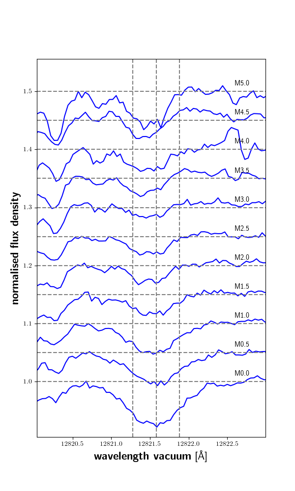
Figure 1: Spectral subtype sequence of the wavelength region around the Pa$\beta$ line for stars with H$\alpha$ in absorption. Spectra of stars later than M5.0 V are not shown, since they either show H$\alpha$ emission or have a low signal-to-noise. Each normalised spectrum is offset for convenience (offset marked as a horizontal dashed line). The dashed vertical lines mark the central wavelength of the Pa$\beta$ line and the lower and upper limit of the line integration band. From bottom to top the following stars are shown: J03463+262 / HD 23453 (M0.0 V), J02222+478 / BD+47 612 (M0.5 V), J00051+457 / GJ 2 (M1.0 V), J13196+333 / Ross 1007 (M1.5 V), J01013+613 / GJ 47 (M2.0 V), J00389+306 / Wolf 1056 (M2.5 V), J02015+637 / G 244-047 (M3.0 V), J12479+097 / Wolf 437 (M3.5 V), J04311+589 / STN 2051A (M4.0 V), J08119+087 / Ross 619 (M4.5 V) J18165+048 / G 140-051 (M5.0 V).

The CARMENES instrument does not cover the Pa $\alpha$ line at 18756.4 Å, but all other members of the Paschen series are covered, including Pa 5 (Pa$\beta$) at 12 821.578 Å, Pa 6 (Pa $\gamma$) at 10 941.17 Å, and Pa 7 (Pa $\delta$) at 10 052.6 Å. The Paschen series ends at about 8250 Å, which is located already in the VIS channel of CARMENES. O₂ airglow lines are found near the Pa$\beta$ line at (vacuum) wavelengths of 12 819.46, 12 822.43, 12 824.78 Å, with the latter line being the strongest (Oliva et al., 2015).

3 Analysis of activity indicators and flare detection

3.1 pEW measurements of activity indicators

To assess the activity state of the stars in each spectrum, we employed pEW measurements. The spectra of M dwarfs do not show an identifiable continuum because of the abundance of molecular absorption lines. These pEW measurements were then used to search for flares in H$\alpha$ and Pa$\beta$.

To give an overview of the appearance of the Pa$\beta$ line, we show examples of it along the M dwarf sequence in Fig. 1 for stars with H$\alpha$ in absorption. In this sequence, the strongest Pa$\beta$ absorption is observed in the M0.0 star. Absorption subsequently weakens until a minimum is reached for the shown M3.5 star, after which the Pa$\beta$ lines deepens again; a more detailed discussion is provided in Sect. 4.1.

To quantify the level of absorption or emission in the lines, we computed pEWs of the H$\alpha$ line, the bluest and middle lines of the Ca ii IRT, as well as the Pa$\beta$, Pa$\gamma$, and Pa$\delta$ lines. We considered H$\alpha$ to be in absorption if the pEW value was larger than $-0.6$ Å, while lower values marked H$\alpha$ in emission. This threshold was already used by Fuhrmeister et al. (2019) and is in between other adopted values as $-0.5$ Å (Jeffers et al., 2018) or $-0.75$ Å (West et al., 2011). If H$\alpha$ is in absorption or emission has traditionally been used to discriminate between inactive or active stars and we also use it here to split up our sample in this sense.

For the pEW computation, we list the central wavelength, full width of the line integration window, and the location of the two reference bands in Table 1; for a more detailed description of pEW measurements of chromospheric lines we refer to Fuhrmeister et al. (2023). While the reference bands are typically blue- and redward of the central wavelength, both are located blueward for the Pa$\beta$ line, since it is located near the red edge of one of the spectral CARMENES orders and we did not want to use a reference band in a different order. While we used $1.5$ Å  wide line integration bands for the Pa$\gamma$ and Pa$\delta$ lines, we opted for a narrower 0.6 Å  wide integration band of Pa$\beta$ to minimize contamination by airglow. This is similar to the even narrower 0.5 Å  band used by Schöfer et al. (2019) for Pa$\beta$. The widths of 1.6 Å  and 0.5 Å  for the H$\alpha$ and Ca ii IRT lines were also used by Fuhrmeister et al. (2020).

For all studied lines, emission during flares may be broader than the line integration band. Therefore, in extreme cases, the full variability range may not be represented with our choice of integration ranges. Moreover, rotation rates higher than about $v\,\sin i=15$ km s^-1 will affect the pEW measurements by shifting flux out of the integration bands (this threshold is exceeded by 20 of our sample stars). Nevertheless, we found the chosen integration bands be suitable for identifying variability, which we are most interested in.

Table 1: Parameters (vacuum wavelength) of the pEW calculation.

Line	Wave-	Width	Reference	Reference
	length		band 1	band 2
	[Å]	[Å]	[Å]	[Å]
H$\alpha$	6564.60	1.6	6537.4–6547.9	6577.9–6586.4
Ca ii IRT1	8500.35	0.5	8476.3–8486.3	8552.4–8554.4
Ca ii IRT2	8544.44	0.5	8576.3–8486.3	8552.4–8554.4
Pa$\beta$ (Pa 5)	12821.58	0.6	12812.0–12814.0	12789.0–12792.0
Pa$\gamma$ (Pa 6)	10941.17	1.5	10902.0–10904.0	10964.7–10966.7
Pa$\delta$ (Pa 7)	10052.60	1.5	10045.0–10047.0	10076.0–10078.0

Table 2: Measured pEWs, their MADs, and stellar parameters.^a

Karmn	Name	SpT	$T_{\mathrm{eff}}$	log g	pEW(H$\alpha$)	pEW(Pa$\beta$)	pEW(Pa $\gamma$)	pEW(Pa $\delta$)	MAD(H$\alpha$)	MAD(Pa$\beta$)	MAD(Pa $\gamma$)	MAD(Pa $\delta$)	$P_{\mathrm{rot}}$	$v\,\sin(i)$
			[K]		[Å]	[Å]	[Å]	[Å]	[Å]	[Å]	[Å]	[Å]	[day]	[km s-1]
J00051+457	BD+44 4548	1.0	3773.0	5.07	0.350	0.024	0.000	0.065	0.016	0.002	0.000	0.002	15.37	2.0
J00067-075	GJ 1002	5.5	3169.0	5.20	-0.043	0.032	0.014	0.265	0.061	0.002	0.005	0.004	0.00	2.0
J00162+198E	LP 404-062	4.0	3329.0	4.93	0.139	0.010	0.081	0.119	0.013	0.003	0.004	0.004	105.00	2.0
J00183+440	GX And	1.0	3603.0	4.99	0.318	0.007	0.032	0.059	0.006	0.001	0.008	0.002	45.00	2.0
J00184+440	GQ And	3.5	3318.0	5.20	0.160	0.014	0.013	0.137	0.010	0.001	0.003	0.002	0.00	2.0
J00286-066	GJ 1012	4.0	3419.0	4.81	0.168	0.007	0.040	0.094	0.008	0.002	0.003	0.002	0.00	2.0
J00389+306	Wolf 1056	2.5	3551.0	4.90	0.287	0.008	0.025	0.076	0.013	0.003	0.004	0.002	50.20	2.0
J00570+450	G 172-030	3.0	3488.0	5.04	0.166	0.012	0.015	0.105	0.024	0.002	0.037	0.003	0.00	2.0
J01013+613	GJ 47	2.0	3564.0	5.05	0.250	0.013	0.026	0.081	0.036	0.002	0.007	0.001	34.70	2.0
J01019+541	G 218-020	5.0	3070.0	5.12	-4.200	0.007	0.018	0.242	0.451	0.003	0.004	0.004	0.14	30.6

^a The full table is provided at CDS. We show here the first ten rows as a guidance.

3.2 Search for Paschen and H$\alpha$ line flares

To study the Paschen lines during flares, flares with a reaction of the Paschen lines need to be identified in the first place. The CARMENES observing schedule does rarely produce consecutive spectra of the same star, but observations of the same star are typically separated by some days.

To facilitate a flare search, we computed for each star the median, $\mu$, of the pEW measurements for each chromospheric line and the median average deviation about the median (MAD). We list these values together with some basic stellar parameters in Table 2 for each star. The MAD yields a robust estimator of the standard deviation. If MAD(pEW(H$\alpha$)) and $\sigma(\mbox{pEW(H$\alpha$)})$ denote the MAD and standard deviation of the time series of pEW measurements of H$\alpha$

$$\sigma(\mbox{pEW(H$\alpha$)})=1.4826\times\mbox{MAD(pEW(H$\alpha$))}\;.$$ (1)

The same nomenclature is used for the other lines.

In a first step, we searched for flares indicated by H$\alpha$ and the Ca ii IRT lines. We accepted a spectrum as flaring (and call this an H$\alpha$ flare) in case of combined H$\alpha$ and Ca ii IRT excursions, viz.,

(i) pEW(H$$\alpha <\mu(\mbox{pEW(H$\alpha$)})-3\sigma(\mbox{pEW(H$\alpha$)})\;\;\;\mbox{and}$$)

(ii) pEW(Ca IRT_1,2) $$<\mu(\mbox{pEW(Ca\leavevmode\nobreak\ IRT${}_{1,2}$)})\,-$$

$$\phantom{<<}3\sigma(\mbox{pEW(Ca\leavevmode\nobreak\ IRT${}_{1,2}$)})\;,$$

where the condition (ii) must apply to at least one of the considered Ca ii IRT lines. Using only the H$\alpha$ line in the search worked well for inactive stars, which exhibit pronounced but seldom flares and show a rather stable H$\alpha$ absorption line otherwise, but not for stars showing persistent, strong variability in H$\alpha$. Since for many of these stars, the Ca ii IRT lines showed less pronounced variations outside of flares, we coupled the search for flares showing up in H$\alpha$ to Ca ii IRT.

Flares also showing up in the Pa$\beta$ line were identified by requiring that condition (i) and (ii) are met, (i. e. the star is flaring in H$\alpha$) and an equivalent $3\sigma$ condition for the pEW of the Pa$\beta$ line is fulfilled. In these so identified Pa$\beta$ flares we additionally searched for Pa$\gamma$ and Pa$\delta$ flares, applying the $3\sigma$ condition one more time.

By this method, most cases of spurious flares induced by statistical noise are suppressed. Additionally, the coupling with an H$\alpha$ criterion removes spurious flares caused by airglow contamination in Pa$\beta$. We nevertheless inspected all Pa$\beta$ flare detections by eye. In the follwoing we call all Pa$\beta$ flares fulfilling our flare criteria ’automatically detected’ and flares that pass the visual inspection ’visually confirmed’.

4 Results and discussion

4.1 The Paschen lines during quiescence

4.1.1 Origin of the Paschen lines

In Fig. 1, we show examples of the Pa$\beta$ line for inactive stars along the M dwarf spectral sub-type sequence. The line is purely chromospheric in origin as can be seen from a comparison to PHOENIX photospheric models (Hauschildt et al., 1999; Husser et al., 2013; Schweitzer et al., 2019), which we show in Fig. 15. The line is absent in photospheric spectra. Moreover, it can be seen in Fig. 1 that around spectral type M2.0 V another absorption feature blueward of the Pa$\beta$ line at about 12821.4 Å  starts to emerge, deepening for later spectral types. The feature can also be seen in the PHOENIX photospheric spectrum for the M5.0 V star shown in Fig. 15, although it is not as deep as observed, which is not uncommon for a molecular feature.

Concerning the origin of the Paschen lines, we distinguish between the lines observed in absorption or in emission. Cram & Mullan (1979) found that for the H$\alpha$ line the line source function is controlled by photoionization (and recombination) for cases where it is in absorption. Therefore, the $n=3$ level as groundstate of the Pa$\beta$ line is populated by H$\alpha$ absorption and by recombination. On the other hand, for flaring states, where we found the line in emission, it must be collisionally controlled, as Cram & Mullan (1979) argued for H$\alpha$ as well.

4.1.2 The Paschen lines along the M dwarf spectral sequence

To generalise the impression from the example sequence in Fig. 1, we show in Fig. 2 the distribution of all median(pEW(Pa$\beta$)) per star as a function of the effective temperature $T_{\rm eff}$, adopted from Cifuentes et al. (2020, from spectral energy distribution fitting) and Marfil et al. (2021, from spectral synthesis). Fig. 2 shows that the Pa$\beta$ line becomes shallower (i.e., yields lower pEWs) for lower $T_{\rm eff}$ (or later spectral type) until a turning point is reached at about $T_{\rm eff}<3400$ K, which corresponds to spectral types of about M4.0 V.

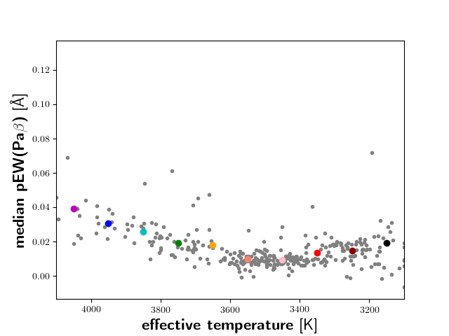
Figure 2: pEW(Pa$\beta$) shown as a function of $T_{\rm eff}$. Grey dots represent median(pEW(Pa$\beta$)) for each star, the coloured circles represent the mean of these median(pEW(Pa$\beta$)) measurements for each $T_{\rm eff}$ interval as introduced in the main text. The colours are chosen as in Figs. 3 and 5 to simplify comparison.

In Fig. 3 we compare the median observed pEWs of the H$\alpha$ and Pa$\beta$ lines of all 360 sample stars. $T_{\rm eff}$ is shown colour-coded in 100 K intervals, to emphasise the temperature dependence of the Pa$\beta$ line. Looking at the stars with H$\alpha$ in absorption (pEW(H$\alpha$ ¿ $-0.6$ Å; which we call inactive stars for the purpose of this study) in Fig. 3, an anti-correlation between $\mu$(pEW(Pa$\beta$)) and $\mu$(pEW(H$\alpha$)) can be noticed for each effective temperature interval. To quantify this impression, we calculated Pearson’s correlation coefficients, $r$, for these samples, and obtained values between $-0.42$ and $-0.91$ with p-values between 0.05 and $10^{-5}$, for 4000 K $>$ $T_{\rm eff}>$ 3200 K indicating fair to highly significant correlations. Only for the highest temperature interval with $r=-0.45$ and $p=0.13$ and for the lowest temperature interval with $r=0.44$ and $p=0.08$ correlations are questionable (and would be positive for the lowest temperature stars). Thus, in general more absorption in H$\alpha$ is on average associated with less absorption in Pa$\beta$ in the stars with H$\alpha$ in absorption for most temperatures. Since in our stellar sample typically a larger pEW(H$\alpha$) is connected to less activity, the Pa$\beta$ line deepends for higher activity levels for the here considered inactive stars. This finding is in line with the analysis by Schöfer et al. (2019).

Stars with H$\alpha$ in emission (which are called active stars traditionally) are only available in meaningful numbers in our sample for $T_{\rm eff}<3400$ K and there is no comparable correlation for these; only for the $3200<T_{\rm eff}<3300$ K interval we find a fair correlation with $r=0.52$ and $p=0.01$, the other two temperature intervals show no correlation with $r$ between $-0.03$ and 0.15 and $p>0.40$. Nevertheless, for stars with $T_{\rm eff}>$3600 K, the pEW(Pa$\beta$) increases further for stars with H$\alpha$ in emission compared to the pEW(Pa$\beta$) of stars with H$\alpha$ in absorption. For stars with $3200<T_{\rm eff}<3600$ K and H$\alpha$ in emission, pEW(Pa$\beta$) saturates at the highest values found for stars with H$\alpha$ in absorption. For stars with $T_{\rm eff}<3200$ K saturation effects play a role for some of the stars, while others show higher or lower values of pEW(Pa$\beta$).

Generally, for the coolest stars in our sample, the spread in pEW(Pa$\beta$) is largest. Moreover, for these stars the most inactive stars with the lowest pEW(Pa$\beta$) values may be not present causing the mean apparent re-deepening of the Pa$\beta$ line together with the additional absorption feature at 12821.4 Å. Nevertheless, as can be seen in Figs. 2 and 3, some of the coolest stars resume the trend to lower pEW(Pa$\beta$). These low values are found in more active stars and we interpret this as fillin-in of the line suggesting that the Pa$\beta$ line is very sensitive to the pressure in the chromosphere.

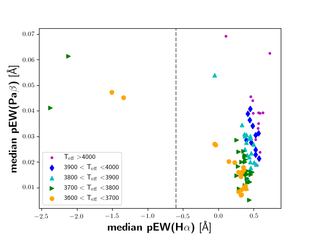
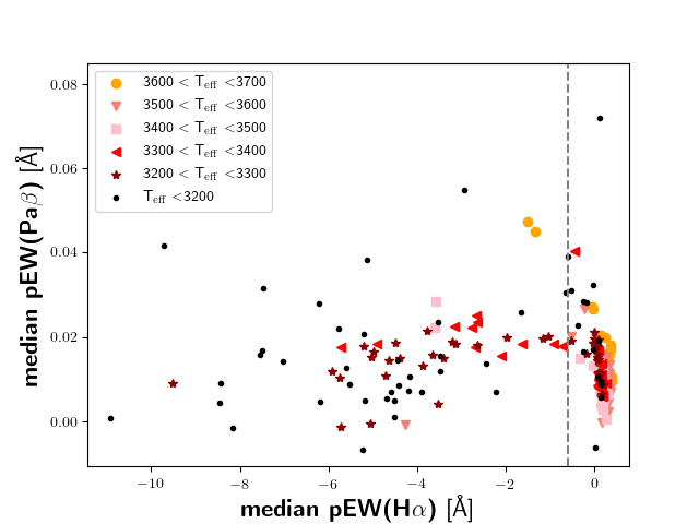
Figure 3: Median(pEW(Pa$\beta$)) shown in relation to median(pEW(H$\alpha$)) with effective temperature of the stars colour-coded as shown in the legend. Left: Stars with high effective temperature. Right: Stars with low effective temperature. For better comparison we show stars with $3600<T_{\rm eff}<3700$ K (orange circles) in both panels. The dashed vertical line marks the dividing line between active and inactive stars.

For 187 stars of our sample a rotational period is known. We therefore compare also the median(pEW(Pa$\beta$)) to the rotational period for these stars (see Fig. 4). As discussed above, for the stars with higher effective temperature, which are generally more inactive, a deepening of the Pa$\beta$ line can be noticed towards shorter rotation periods (i. e. higher activity levels). Only for the coolest stars deepening and fill-in or saturation is observed as one proceeds to shorter periods.

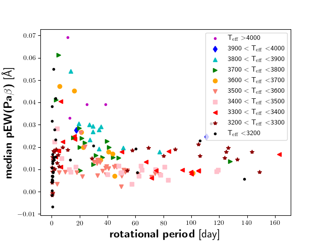
Figure 4: Median(pEW(Pa$\beta$)) shown in relation to the rotation period with effective temperature of the stars colour-coded as shown in the legend.

4.1.3 Time series of individual stars

To study the relation between the pEWs measured in the H$\alpha$ and Pa$\beta$ lines in individual stars, we also computed Pearson’s correlation coefficients for the time series of pEW(H$\alpha$) and pEW(Pa$\beta$) on a by-star basis and show the resulting values of $r$ in Fig. 5, where significant results (p $<$ 0.005) are highlighted by colour. Stars with H$\alpha$ in emission tend to show a significant positive correlation between pEW(H$\alpha$) and pEW(Pa$\beta$), while stars with H$\alpha$ in absorption more often show significant anti-correlation. The latter cases are mostly stars with $T_{\rm eff}>$3400 K, while the former are usually cooler stars, and one should keep in mind that our sample contains few stars with $T_{\rm eff}>$3400 K and H$\alpha$ in emission. Also, many of the stars showing positive correlations are affected by flaring activity in the Paschen lines (see Sect. 4.2.1), which often dominates the variability in pEW(Pa$\beta$) and, thus, drives the correlation.

Moreover, it is an interesting question, if detectable rotational modulation is imprinted on the Pa$\beta$ time series. We therefore computed a generalized Lomb-Scargle periodogram (Zechmeister & Kürster, 2009) for the Pa$\beta$ time series and accepted periods between 1.5 and 150 days and a false-alarm probability smaller than 0.005 as significant rotational modulation. We found six stars fulfilling these criteria, which we list in Table 3. For three of these stars, there is no known rotation period. For one star a conflicting rotation period is known; for another star (J16343+571 / CM Dra; spectral type M4.5 V, eclipsing binary) we found a period of 2.4 days, while a period of about half this value of 1.27 days is known for this star for the mutual orbital period (Doyle et al., 2000). For the last star (J03133+047 / CD Cet; spectral type M5.0 V) we found a period of 127.2 days, while a period of 126.2 days was determined by Newton et al. (2016). A more detailed study found a period of $170^{+19}_{-38}$ days using photometry and about 134 days using spectroscopy (Bauer et al., 2020). These findings show again that the Pa$\beta$ line is sensitive to activity, but not as sensitive as other tracers. This may – especially for period search – be partly caused by the problems of obtaining pEWs free of the influence of telluric and airglow lines or the artefacts from their removal. Anyway, rotational modulation in M dwarfs is traced best with photometric variations (Irwin et al., 2011; West et al., 2015; Suárez Mascareño et al., 2016; Díez Alonso et al., 2019).

Table 3: Detectable rotation in Pa$\beta$.

star	detected	literature	ref
	period	period
	[days]	[days]
J00184+440	6.6	…
J00403+612	119.3	…
J03133+047	127.2	126.2	New16
J04167$-$120	135.6	…
J11511+352	94.0	22.8 $\pm$ 1.0	DA19
J16343+571	2.4	1.27	Dev08

DA19: Díez Alonso et al. (2019); Dev08: Devor et al. (2008); New16: Newton et al. (2016)

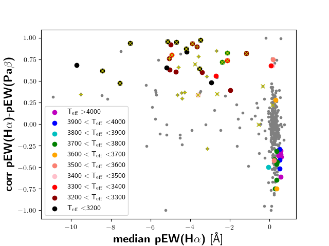
Figure 5: Pearson correlation coefficient $r$ between pEW(H$\alpha$) and pEW(Pa$\beta$) shown as a function of $\mu$(pEW(H$\alpha$)). $T_{\rm eff}$ is colour coded as shown in the legend for stars with a significant Pearson correlation (p $<$ 0.005). Stars with automatically or visually found flares (see Sect. 4.2.1) are marked with crosses and plusses, respectively.

4.2 Flaring activity found in H$\alpha$ and the Paschen lines

4.2.1 Overview

Applying the automatic flare search described in Sect. 3.2, we found 357 H$\alpha$ flares in 153 stars, and 46 Pa$\beta$ flares in 30 stars. We summarize these and all the numbers in this Section in Table 4. We examined all Pa$\beta$ flares by eye and removed 11 for which we found airglow to remain a problem. The other stars all show the Pa$\beta$ line in emission. This excludes confusion with high amplitude rotational modulation, since Pa$\beta$ emission certainly involves high pressure, see also the discussion in Sect. 4.2.3. For these stars we automatically detect 15 stars with 24 Pa$\gamma$ flares and 15 stars with 24 Pa$\delta$ flares. These are not the same, though. While for most flares with Pa$\gamma$ emission, Pa$\delta$ emission is also detected, there are six flares, where no Pa$\delta$ was detected. There are another six flares, where Pa$\delta$ was detected despite no Pa$\gamma$ emission. For these latter six flares the Pa$\delta$ detection is correct and Pa$\gamma$ was not detected due to noise in some spectra of the three affected stars, which enlarges the MAD incorrectly and hinders the automatic Pa$\gamma$ detection. Therefore we manually correct the number of Pa$\gamma$ flares to 30 flares in 18 stars. As a typical example of the outcome of the automatic search, we show in Fig. 6, the M3.5 star J07319+362N / BL Lyn. Both, the Pa$\beta$ and the Pa$\gamma$ lines can be seen in broad emission exceeding 5 Å. Other spectral features in the region are still imprinted on the broad emission lines. The (about) Gaussian shape of these lines is revealed by spectral subtraction of the quiescent spectrum (see Sect. 4.2.4).

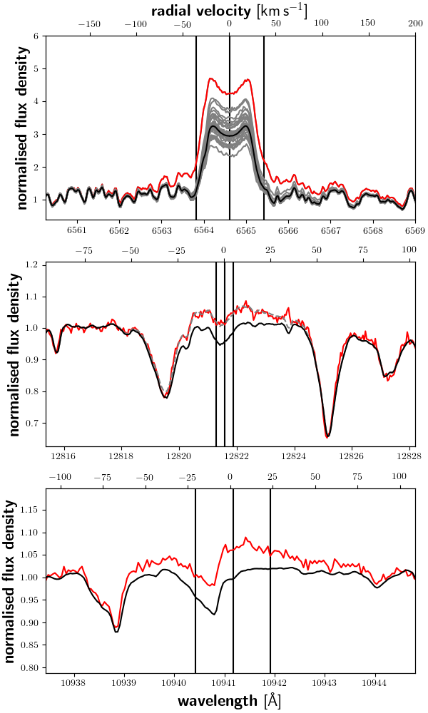
Figure 6: Typical example of flaring activity: the M3.5 V star J07319+362N / BL Lyn. Top: The H$\alpha$ line. Middle: The Pa$\beta$ line. Bottom: The Pa$\gamma$ line. Shown are all spectra of the star in grey (only for H$\alpha$ for clarity), and the median spectrum in black, while the flare spectrum is shown in red. For the Pa$\beta$ line we also show as grey dashed line a Gaussian fit of the flare excess flux density. The vertical lines denote the central wavelength of the respective line and the integration ranges of the pEWs. During flares showing Pa$\beta$ emission, the integration range for the Paschen lines as well as the H$\alpha$ line is usually much too small and can only be used for identification of these flares. In the shown example the full width at the line footpoints exceeds 5 Å  for all three shown lines. For more details, see Sects. 3.1 and 4.2.4

An additional visual inspection of the stars with automatic Pa$\beta$ flare detections yielded another six small Pa$\beta$ flares in four of the stars. Therefore, especially lower amplitude Pa$\beta$ flares may be missed by the automatic detection, and we therefore screened our whole sample also by eye. Thus, we identified 12 additional stars with 16 small Pa$\beta$ flares. We show an example spectrum of a visually found Pa$\beta$ flare in Fig. 16. Generally, these visually found flares are comparable in strength to the smallest flares found by the automatic detection, and the reasons why they were missed are manifold. One star, for instance, shows a large red asymmetry, which shifts the Pa$\beta$ emission out of the integration range. In other cases, the low number of spectra, large ranges of variability, and airglow or a combination thereof confound the search. This altogether leaves us with 32 stars showing 57 Pa$\beta$ flares in comparison to 153 stars showing 357 H$\alpha$ flares. Since our flare classification relies on relative variation based on the MAD of the time series, we show in Fig. 7 also the absolute deviation of the flare related pEW(Pa$\beta$) measurements compared to the median of pEW(Pa$\beta$). We caution that these values are systematically underestimated, since our pEW integration range is not broad enoug to cover the whole line during the flare. Nevertheless, flares with $\Delta$pEW(Pa$\beta$)$>0.03$ Å  are typically detected automatically, while for smaller flares a non-detection by the search algorithm gets more probable. Furthermore, we note that some of the detected Paschen flares have been touched upon in the literature in the context of studies of other lines (Fuhrmeister et al., 2018, 2020), but no detailed discussion of the specific properties of the Paschen lines was provided there.

Table 4: Summary of found flares.

method	no. of	no. of	no. of	no. of
	Pa$\beta$	Pa$\gamma$	Pa$\delta$	H$\alpha$ flaresa
	flaresa	flaresa	flaresa
automatically	46 (30)	29 (20)	27 (17)	357 (153)
after vis. exclusion
of false positives	35 (20)	24 (15)	24 (15)
after correction for
noise in Pa$\gamma$		30 (18)
additionally visually
found flares	6 (4)b
add. vis. found
flares (whole sample)	16 (12)
total	57 (32)	30 (18)	24 (15)	357 (153)

^a The number of stars in which these flares are detected is given in parenthesis.
^b In the stars with automatically Pa$\beta$ flare detection

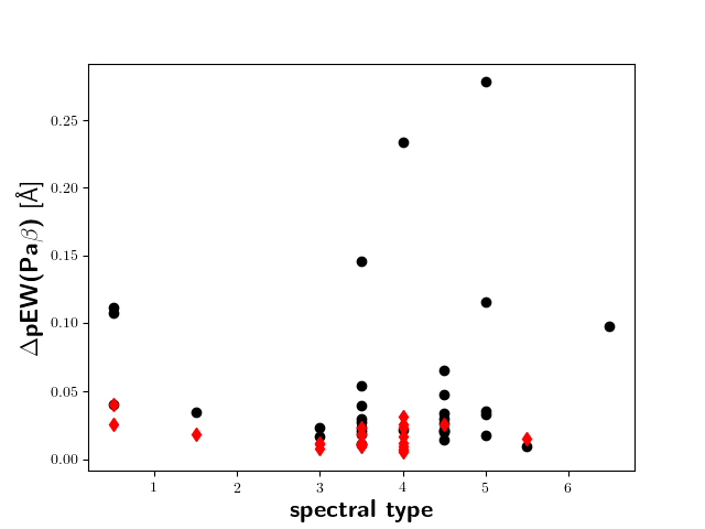
Figure 7: Deviation of the flare related pEW(Pa$\beta$) from the median of the pEW(Pa$\beta$) of the respective time series for the automatically detected flares (black dots) and the visually found flares (red diamonds). We caution that $\Delta$pEW is systematically understimated, since the integration width is not broad enough to cover the flaring line.

4.2.2 Statistical properties of the Pa$\beta$ flares

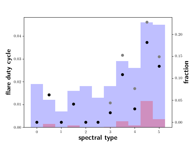
Figure 8: Flare duty cycle (flare time fraction, left y-axis) of H$\alpha$ (blue bars) and Pa$\beta$ flares (red bars) for automatically detected flares along with fractions of stars per spectral subtype (right y-axis) with automatically detected Pa$\beta$ flares (black dots) and all Pa$\beta$ flares (i. e. including visually found flares; grey dots). The fractions of flaring stars for spectral types M0.5, M1.5, and M3.0 each correspond to a single star with a flare detection.

The accumulated exposure time of all spectra considered here is 213.02 days. Comparison with the total exposure time for spectra with automatically detected H$\alpha$ flares leads to a “flare duty cycle” (Hilton et al., 2010) of $2.26$ %. In contrast, the flare duty cycle for automatically detected Pa$\beta$ flares, with all cases of airglow contamination excluded by visual inspection, is only $0.19$ %, about an order of magnitude smaller.

In Fig. 8, we show the flare duty cycle as a function of spectral subtype for automatically detected H$\alpha$ and Pa$\beta$ flares, which increases toward later type stars for both lines. For H$\alpha$ flares, such an increase was already described by Hilton et al. (2010), who found, however, lower duty cycles of 0.02 % for early M stars and 3 % for late M dwarfs in time resolved spectra of the Sloan digital sky survey. We ascribe these different numbers to the different sensitivities and flare detection methods.

Additionally, we show in Fig. 8 the fraction of Pa$\beta$ flare stars as a function of the spectral subtype. The detected Pa$\beta$ flares are clearly concentrated on stars of later spectral types, since only three stars of type M3.0 V and earlier show Pa$\beta$ flares, while the remaining 17 stars with automatically detected Pa$\beta$ flares are of spectral type M3.5 V and later.

Moreover, all but three stars with detected Pa$\beta$ flares clearly show H$\alpha$ in emission. The three stars with H$\alpha$ absorption are J11476+786/GJ 445, J02070+496 / G 173$-$037, and J23351$-$023 / GJ 1286, out of which the latter two are in a transition state, where H$\alpha$ is neither in clear absorption nor emission. We show the flaring spectra of all of these three stars in Figs. 17, 18, and 19.

We also compare the flare duty cycle of all active stars, which we found to be 4.7 % for H$\alpha$ and 1.0 % for Pa$\beta$, while for the inactive stars it is 2.2 % for H$\alpha$ and 0.03 % for Pa$\beta$. These numbers are comparable to the values for mid-type M dwarfs and early-type M dwarfs, since there are very few early-type M dwarfs among the active stars, while the mid-type M dwarfs have many active stars among them. Moreover, we compute the flare duty cycle only considering the stars flaring in H$\alpha$. Then the flare duty cycle becomes 4.0 % for H$\alpha$ and 0.3 % for Pa$\beta$.

4.2.3 Stark broadening in H$\alpha$ for Pa$\beta$ flares

Of the spectra exhibiting Pa$\beta$ emission, the vast majority shows relatively symmetric H$\alpha$ line broadening. In their analysis of line asymmetries, Fuhrmeister et al. (2018) reported that red asymmetries occur frequently, blue asymmetries are more rarely observed, and symmetric line broadening is the most rarely observed variant, which is only about half as frequent as red asymmetries. Therefore, we consider a chance finding unlikely and conclude that Pa$\beta$ emission is likely coupled to the occurrence of symmetric broadening. Like other authors such as Kowalski et al. (2017) and Wu et al. (2022), we consider Stark (pressure) broadening the most plausible explanation for the rather symmetric line profiles, which may alternatively be attributed to turbulent broadening or an observational time integration effect, caused by the blurring of a blue and a red asymmetry during the exposure.

Stark broadening is a consequence of high pressure in the chromosphere and, therefore, is expected to be associated with material showing larger collision rates, which lead to a larger population of higher hydrogen excitation levels. Consequently, we attribute the Pa$\beta$ line emission during flares to high pressures in the chromosphere and lower transition region. Notably, flares with comparable or even higher amplitudes in H$\alpha$ but no line broadening lead to Paschen line emission as exemplified by the case shown in Fig. 9, where the higher amplitude flare marked in blue does not show H$\alpha$ broadening and also no enhancement of the flux in the Paschen lines. If anything, marginal excess absorption may be present in Pa$\beta$ during this flare. We caution, nevertheless, that Stark broadening of the H$\alpha$ line does not necessarily lead to Paschen line emission. A case in point was presented by Paulson et al. (2006), who reported on Stark broadening of the Balmer lines during a flare on the M4.0 M dwarf Barnard’s star, but did not detect Paschen line emission, although they covered Pa$\delta$ and higher.

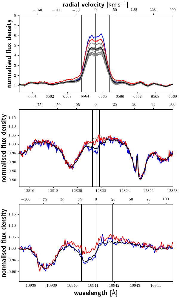
Figure 9: Same as Fig. 6 but for the M4.5 V star J07558+833/GJ 1101. Two flares are marked as red and blue spectra, but only one leading to Pa line emission.

4.2.4 H$\alpha$ and Pa$\beta$ line profiles during flares

Since the pEW(Pa$\beta$) is measured using a narrow integration band (see Table 1), it captures only a fraction of the flux if the line is broad. Likewise, the H$\alpha$ line also exceeds the integration width used to obtain its pEW during many of the observed flares. Therefore, the pEW values do not fully characterise the strengths of broad lines.

To obtain a better understanding of the line profiles during flares, we first obtained excess spectra by subtracting the median spectrum from the flaring spectrum and, subsequently, fitted the resulting lines using Gaussians. Specifically, we used a narrow and a broad Gaussian component for the H$\alpha$ line as we did in Fuhrmeister et al. (2018) and a single Gaussian component for the Pa$\beta$ line. We list the best-fit parameters of our model for each flare in Table 6 for the automatically detected flares and in Table 7 for all flares found by visual inspection.

The two-Gaussian model reproduces the spectral line shape of H$\alpha$ fairly well. In particular, the two Gaussians can account for mutual shifts of the broad and narrow component, which is a measure of the line asymmetries. For the Pa$\beta$ line, we used a single Gaussian model, which is appropriate in most cases. There are eight Pa$\beta$ flares, where the fit of the excess flux in Pa$\beta$ was not adequate. Six of these are visually found flares, where a combination of low amplitudes and high width prevents a good fit. For some of the visually found flares also the broad component of H$\alpha$ cannot be fit for similar reasons. Additionally, there are a few examples where a single Gaussian does not seem to be a suitable model for the Pa$\beta$ line profile; these are marked in the Tables 6 and 7.

With these fits we proceeded to investigate the correlation behaviour between the H$\alpha$ and Pa$\beta$ line properties. We found that the strength of the narrow H$\alpha$ component is not correlated with that of the Pa$\beta$ line (Pearson’s $r=0.23$, $p=0.11$). Neither is the total strength of the narrow and broad H$\alpha$ components correlated with that of Pa$\beta$ ($r=0.38$, $p=0.007$). However, the strength of the broad H$\alpha$ component is correlated with that of the Pa$\beta$ line (Pearson’s $r=0.54$ and $p=7.7\cdot 10^{-5}$). Likewise, there are correlations between the width of the broad H$\alpha$ component and that of the Pa$\beta$ line ($r=0.57$ and $p=2.2\cdot 10^{-5}$) and the shift of the broad component of H$\alpha$ and the line shift of Pa$\beta$ ($r=0.51$ and $p=0.0002$). This clearly shows that the broad component of H$\alpha$ and the Pa$\beta$ emission are intimately related during flares and that the emission originates most probably from the same material.

From the Gaussian fits also the luminosity of Pa$\beta$  $L_{\mathrm{\mbox{Pa$\beta$}}}$ can be computed using PHOENIX photospheric models (Husser et al., 2013) for $T_{\mathrm{eff}}$ and $\log g$ and the radius of the respective star (Schweitzer et al., 2019). Using luminosities by Cifuentes et al. (2020) this can be converted into $\log L_{\mathrm{\mbox{Pa$\beta$}}}/L_{\mathrm{bol}}$. We list these values in Tables 6 and 7. Values of $\log L_{\mathrm{\mbox{Pa$\beta$}}}/L_{\mathrm{bol}}$ range from -4.03 to -8.16 but mostly concentrating between -5.5 and -6.5. We caution that these values strongly rely on theoretical assumptions and may therefore have large systematic errors.

4.2.5 Asymmetries in Pa$\beta$ flares

H$\alpha$ often exhibits asymmetric line profiles during flares, which can manifest either as blue or red wing emission with various velocity shifts and amplitudes (for asymmetries during flares on M dwarfs see Fuhrmeister et al. (2018), and references therein; for the Sun see for example Berlicki (2007)). Asymmetric H$\alpha$ line spectra during flares are usually attributed to mass motions. Specifically, blue asymmetries are thought to be caused by chromospheric evaporation during flare onsets (Li et al., 2022) or prominence eruption with possible coronal mass ejections (Honda et al., 2018; Notsu et al., 2021). The origin of the red asymmetries is less certain and may, indeed, vary depending on whether the asymmetry is observed during the impulsive or the decay phase of the flare. While red asymmetries may be caused by chromospheric condensations, mainly expected to happen in the impulsive phase, in the decay phase they may be caused by coronal rain (Wu et al., 2022) or are associated with post flare loops (Namizaki et al., 2023).

Looking at the Pa$\beta$ line fits, we selected all spectra showing a shift of more than 15 km s${}^{-1}\,(=0.65$ Å) and found two blue asymmetries and one red asymmetry among the automatically detected flares and additionally three red asymmetries among the visually found flares. Although these are small numbers, there seem to be more red than blue asymmetries, in agreement with what Fuhrmeister et al. (2018) found for H$\alpha$ asymmetries. This seems to indicate again, that the shifted Pa$\beta$ and H$\alpha$ emission originate in the same regions. The low number of spectra with shifted Pa$\beta$ emission (compared to H$\alpha$) seem to indicate, that the pressure is usually not high enough in these regions to produce a measureable amount of Pa$\beta$ emission.

Out of the six detected Pa$\beta$ asymmetries we discuss here the two blue asymmetries and the largest red asymmetry in more detail. While the latter belongs to J01352$-$072 / Barta 161 12, the two blue asymmetries occured on J01033+623 / V388 Cas and J22012+283 / V374 Peg. For all three examples, the Pa$\beta$ lines show large shifts and the line profiles are consistent with only the shifted material showing emission. Therefore, we compared the line shifts (in velocity space) of the broad H$\alpha$ component to the line shift of the Pa$\beta$ component. For J01033+623 / V388 Cas, both are shifted about $-30$ km s^-1 compared to the respective line centre. For J22012+283 / V374 Peg, we find a velocity of $-8.7$ km s^-1 for the broad component of H$\alpha$ and $-16.4$ km s^-1 for Pa$\beta$. For J01352$-$072 / Barta 161 12, we find $147.9$ km s^-1 for H$\alpha$ and $46.7$ km s^-1 for Pa$\beta$. Given that the fit of very broad lines typically produces larger uncertainties on the central wavelength, we consider the velocity shifts for the first two stars to be in agreement. In the case of the red asymmetry, where the difference is about $100$ km s^-1, the broad H$\alpha$ profile may actually be composed of more than one component, which is not accounted for in the modelling and could, thus, explain the difference. We show all three examples in Figs. 10 and 11.

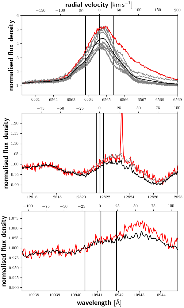
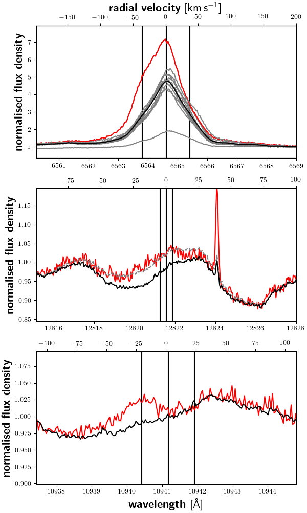
Figure 10: Same as in Fig. 6 but for the M4.0 V star J01352$-$072 / Barta 161 12 (left; not automatically found) and for the M4.0 V star J22012+283 / V374 Peg (right). Both stars are fast rotators with vsini = 59.8 and 36.9 km s^-1, respectively. Both stars display large asymmetries in their H$\alpha$ lines and line shifts in the Pa$\beta$ line.

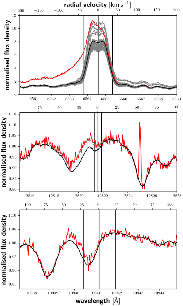
Figure 11: Same as in Fig. 10 but for the M5.0 V star J01033+623 / V388 Cas. The star is a moderately fast rotator with vsini = 10.5 km s^-1. Again, the line shift in Pa$\beta$ corresponds to an asymmetry in the H$\alpha$ line.

There are more example of asymmetric H$\alpha$ line shapes in the spectra of the stars, which exhibit Pa$\beta$ flares at some point during the time series. However, in these instances usually no Pa$\beta$ emission is detectable at all, neither at the nominal wavelength nor at a shift. In these cases, the densities in the moving material are likely too low to produce Pa$\beta$ emission.

4.2.6 Higher Paschen series lines

We visually screened the spectra with detected flares also for lines higher up in the Paschen series. For seven stars, we could find Pa 10 (at 9017.8 Å), Pa 13 (at 8667.40 Å), and Pa 14 (at 8600.75 Å) unambigiously. Pa 13, Pa 15 (at 8547.73 Å), and Pa 16 (at 8504.83 Å) are blended with the wings of the Ca ii IRT at 8500.35, 8544.44, and 8664.52 Å. Pa 17 (at 8469.59 Å) is blended with two Ti i absorption lines at 8469.474 and 8470.797 Å. These Paschen lines are therefore hard to detect, especially next to the broad and highly variable Ca ii IRT lines, which during flares usually show strong emission. We show the two flare spectra of J20451$-$313 / AU Mic and the Pa 14 lines in Fig. 12 and the Pa 14 line of J13536+776 / RX J1353.6+7737 as second example in Fig. 20. We list all stars with detections of Pa 10 or higher in Table 5.

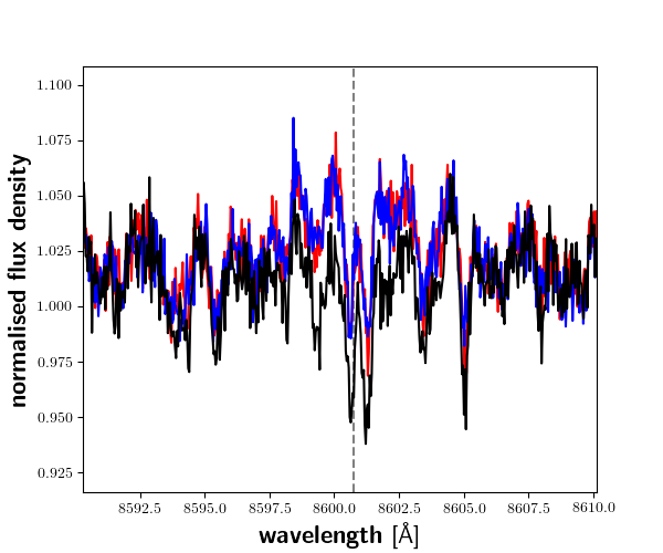
Figure 12: Pa 14 line for the M0.5 V star J20451$-$313 / AU Mic.

These higher Paschen lines have the potential to trace the gas conditions in the chromosphere. A detailed chromospheric modelling with a stellar atmosphere code would yield the best results. This was done for example using PHOENIX (Hauschildt et al., 1999) by Hintz et al. (2020) for the He i infrared triplet. Such a modelling is beyond the scope of this paper and therefore we stick here to a much easier and simpler analysis using the highest observed line, which was also used by Paulson et al. (2006) for a flare on Barnard’s star using hydrogen Balmer lines. The method of a pressure estimate using the highest resolved line is described in Kurochka & Maslennikova (1970). For the flares, where we detected only Pa 10 as highest line, we argue that we are sensitivity limited. Therefore, our highest resolved Paschen line is Pa 13 or Pa 14. Since for these high pressures broadening by the Doppler effect plays a minor role, the Stark effect dominates the broadening, which leads to a merging of the lines. Using Equ. 9 from Kurochka & Maslennikova (1970) leads to $\log n_{e}\leqslant 14.0$. This value compares well with the one found by Paulson et al. (2006) using the same method. It agrees also with the electron pressure found for the higher chromosphere by detailed flare modelling for a flare on CN Leo (Fuhrmeister et al., 2010).

Table 5: Flares with Pa lines higher than Pa 9 detected.

Karmn	JD	highest line
J08298+267	2459177.625451389	Pa 10
J09161+018	2457712.658923611	Pa 10
J11474+667	2457762.5463541667	Pa 13
J13536+776	2458678.4093055557	Pa 14
J15218+209	2457950.498854167	Pa 10
J20451$-$313	2458679.526851852	Pa 14∗
J20451$-$313	2458679.531608796	Pa 14∗
J22468+443	2457633.4671527776	Pa 13

Notes: ^∗: These are consecutive spectra discussed in Sect. 4.2.7.

4.2.7 Consecutive Paschen line flares

There are three Paschen line flares with two consecutive spectra: one flare on YZ Cet and two flares on AU Mic. In the case of YZ Cet, the two spectra were taken about one hour apart. For the flares on AU Mic, the temporal offsets are only 7 min and 14 min. The observed evolution is diverse. For the YZ Cet flare, the combined H$\alpha$ flux of the narrow and broad component decayed by only ten percent within an hour, the Pa$\beta$ line flux approximately halved in the same time. For the first AU Mic flare, the H$\alpha$ emission decayed by about 15 percent in 7 minutes while the Pa$\beta$ emission stayed constant. During the second flare, the H$\alpha$ emission decayed by about 80 percent in 14 minutes, while the Pa$\beta$ emission dropped by about 95 percent. Although the sample is small and the sampling sparse, we conclude tentatively that the Pa$\beta$ emission during flares likely decays as fast as or faster than the H$\alpha$ emission, but not significantly more slowly.

4.2.8 Outstanding examples of Pa$\beta$ line flares

Among the identified Pa$\beta$ flares, there are a number of exceptional examples. We present here the stars with the largest Pa$\beta$ amplitude in our fit (see Table 6). There are six flares with an amplitude larger than 1.0 Å  belonging to four stars. All four stars have rotational periods of less than 15 days and have generally high activity levels.

The star exhibiting the flare with the overall largest amplitude is the M5.0 V star J11474+667 / 1RXS J114728.8+664405, which shows two Pa$\beta$ flares, with also the second flare having a considerable amplitude. We show the two flaring spectra in Fig. 13.

The star with the second highest amplitude is the young M0.5 V star J20451$-$313 / AU Mic, which has three out of four automatically detected flares among the large amplitude flares. This is also the star of earliest subtype exhibiting a Pa$\beta$ flare and all three large Pa$\beta$ flares of this star have the three broadest Pa$\beta$ lines found. We show the flaring spectra in Fig. 14.

Also J22468+443 / EV Lac is an exceptional star. It has one flare among the large Pa$\beta$ flares and another three automatically detected Pa$\beta$ flares. Considering the three additional manually identified Pa$\beta$ flares, it is the star with the largest number of Pa$\beta$ flares found (followed by J20451$-$313 / AU Mic). We show five (out of seven) flaring spectra of various strength in Fig. 21. The weakest of these flares shows Pa$\beta$ emission, but no detectable Pa$\gamma$ emission while all other exhibit notable Pa$\gamma$ emission.

The last star with a large amplitude Pa$\beta$ flare is the M4.0 V star J13536+776 / RX J1353.6+7737. The spectra are shown in Fig. 22. J13536+776 / RX J1353.6+7737 displays a second Pa$\beta$ flare, which is quite a small one and cannot be fitted properly.

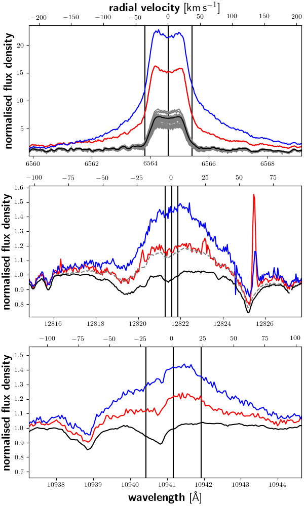
Figure 13: Same as in Fig. 6 but for Pa$\beta$ flares on the M5.0 V star J11474+667 / 1RXS J114728.8+664405. Each coloured spectrum corresponds to one Pa$\beta$ flare.

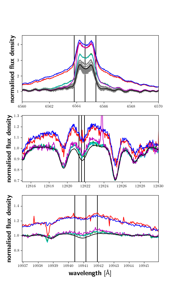
Figure 14: Same as in Fig. 6 but for Pa$\beta$ flares on the M0.5 V star J20451$-$313 / AU Mic. Each coloured spectrum corresponds to one Pa$\beta$ flare.

5 Summary and conclusions

In our study we analysed the Paschen lines, which are purely of chromospheric origin, in a sample of 360 M dwarfs, which provide together more than 19 000 CARMENES spectra. We specifically used the pEW(H$\alpha$) and pEW(Pa$\beta$) to characterise the behaviour of the Pa$\beta$ line in non-flaring state along the M dwarf spectral sequence. We found, that on average the Pa$\beta$ line becomes more shallow for later spectral types until about spectral type M3.5; for even later spectral types the line re-deepens. Comparing the pEWs of H$\alpha$ and Pa$\beta$ showed, that for inactive stars with H$\alpha$ in absorption in a certain $T_{\rm eff}$ range, the median(pEW(H$\alpha$)) per star is anti-correlated to the median(pEW(Pa$\beta$)). Only our hottest ($T_{\rm eff}>4000$ K) and our coolest ($T_{\rm eff}<3200$ K) temperature interval showed no correlation. For the active stars with H$\alpha$ in emission, there is in contrast only one $T_{\rm eff}$ interval, where a fair correlation between median(pEW(H$\alpha$)) and median(pEW(Pa$\beta$)) could be found. Nevertheless, for time series measurements of individual stars with H$\alpha$ in emission we often found correlations between pEW(H$\alpha$) and pEW(Pa$\beta$). On the other hand, for time series measurements of pEW(H$\alpha$) and pEW(Pa$\beta$) we found an anti-correlation for many stars with H$\alpha$ in absorption. For both cases – looking at the median values of the stars for comparing the stellar sample and also for looking at time series of individual stars – we caution, that there are no stars with H$\alpha$ in emission for $T_{\rm eff}>3400$K.

Regarding the flaring activity of the sample stars, we found 357 H$\alpha$ flares in 153 stars in comparison to 30 (57) Pa$\beta$ flares in 18 (32) stars with the number in brackets including flares found only by visual inspection. Out of the automatically found Pa$\beta$ flares, 86% and 69 % also show Pa $\gamma$ and Pa $\delta$ in emission. Even higher Pa lines could be found unambigously up to Pa 14 for three flares (9%). The detection of even higher Pa lines is hampered by their blending with the Ca ii IRT or other stronger absorption lines. Since our pEW integration width is chosen mainly to identify flares for further characterization we applied Gaussian fitting to the Pa$\beta$ line. We demonstrate the quality of the Gaussian fit of the flare excess flux density by showing some of these fits in Figs. 6, 9, 10, 11, and 13.

Both, H$\alpha$ and Pa$\beta$ flares are more often found in later spectral types (75% of H$\alpha$ flares and 90% of Pa$\beta$ flares are in stars with spectral type of M3.0 V or later). The ’flare duty cycle’ (as a measure for the time fraction the star spends flaring) also increases for later spectral types, as was found for H$\alpha$ already by Hilton et al. (2010). Moreover, the stars with Pa$\beta$ flares nearly all show H$\alpha$ in emission; only two show H$\alpha$ in a transition state from absorption to emission and one star shows weak H$\alpha$ absorption outside the flares. Therefore, not surprisingly, the stars with the most exceptional flares in amplitude, number and width (which we show in Figs 13, 14, 21 and 22) are well known very active stars as J22468+443 / EV Lac or J20451$-$313 / AU Mic. Additionally, we found some examples of asymmetries in the Pa$\beta$ lines during flares, clearly more often associated with red asymmetries, than with blue ones.

Even more interestingly, Pa$\beta$ emission during flares seems to be coupled to high densities, because almost all cases of Pa$\beta$ flaring occur, when H$\alpha$ exhibits symmetric broadening, which is indicative of Stark broadening (Kowalski et al., 2017) and therefore high densities. Higher amplitude flares without Stark broadening typically do not lead to Pa$\beta$ emission, but Stark broadening in H$\alpha$ also need not to necessarily lead to Pa$\beta$ emission. As an indication of the strong coupling between the broad (Stark) component of the H$\alpha$ line and the Pa$\beta$ emission, we found a correlation between amplitude, width and shift of these. This sensitivity to chromospheric densities of the Pa lines deserves further investigation. For this purpose, dense time series of spectra covering a Pa$\beta$ flare are needed. We identified here a number of promising candidates for such a project. These stars seem to show Pa$\beta$ flares more often than the majority of M dwarfs. Such flare observations would allow to investigate, during which flare stage the Pa$\beta$ emission starts and if there is a time lag to the reaction of H$\alpha$ like seen for other chromospheric lines in flare studies. Together with dedicated chromospheric flare modelling this would lead to a better understanding of the density variation during a flare.

Appendix A Comparison to PHOENIX models

Here we compare the spectral wavelength range around the Pa$\beta$ line of the M0.5 V star J02222+478 / BD+47 612 and the M5.0 V star J18165+048 / G 140-051 (both also shown in Fig. 1) to PHOENIX purely photospheric models from the library of Husser et al. (2013). PHOENIX is a stellar atmosphere code (Hauschildt et al. 1999), which is widely used to compute photospheric stellar models and their synthesised stellar spectra and has been applied to CARMENES spectra to establish stellar parameters (Passegger et al. 2018; Schweitzer et al. 2019; Cifuentes et al. 2020; Marfil et al. 2021). We use a model with $T_{\rm eff}$=3900 K for the M0.5 star, a model with $T_{\rm eff}$=3200 K for the M5.0 star and $\log g$=5.0 in both cases. Marfil et al. (2021) listed $T_{\rm eff}=3894\pm$11 K and 3240$\pm$36 K and $\log g=4.99\pm$0.09 and 4.97$\pm$0.13, for the two stars, respectively. In Fig. 15 the generally good resemblance for both spectra can be seen. Although there are some weaker lines in the PHOENIX spectra which are not seen in the observed spectra and vice versa, the stronger atomic lines match quite well. However, the Pa$\beta$ line is not present in the PHOENIX spectra, making it evident, that it is a purely chromospheric line.

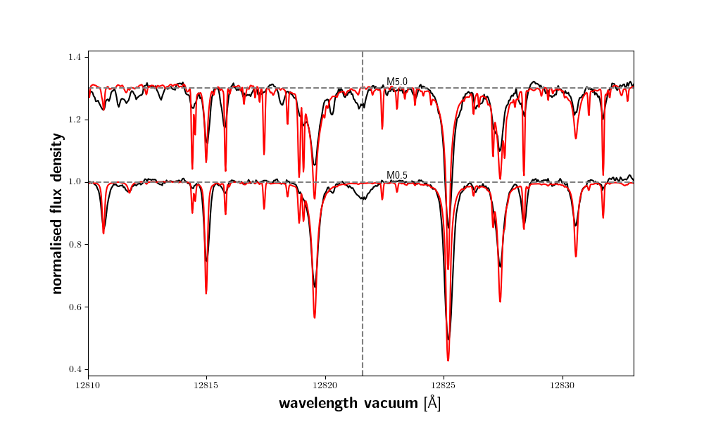
Figure 15: Spectral comparison to PHOENIX photospheric models for Pa$\beta$. Shown are the normalized spectra of the M0.5 V star J02222+478 / BD+47 612 and the M5.0 V star J18165+048 / G 140-051 from Fig. 1 as black solid line with an offset indicated by the grey dashed line. In red PHOENIX photospheric comparison spectra are shown. The vertical dashed line marks the position of the Pa$\beta$ line.

Appendix B Further examples of Pa$\beta$ line flares

We show here further examples of Pa$\beta$ line flares. In Fig. 16 we show an example of a flare not found by our automatic detection, but only by visual inspection. In Figs. 17, 18, and 19 we show the flare spectra for the three stars with H$\alpha$ not in clear emission. We show a further example of the Pa 14 line in Fig. 20. In Figs.  21, and 22 we show the outstanding flares, which we described in Sect. 4.2.8.

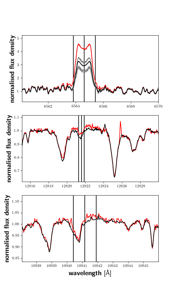
Figure 16: Same as in Fig. 6 but for a Pa$\beta$ flare not found automatically for the M4.0 V star J12428+418 / G 123-055. There are only few spectra available for the star and the variation is high, which prevents the program to automatically detect the relatively small flare.

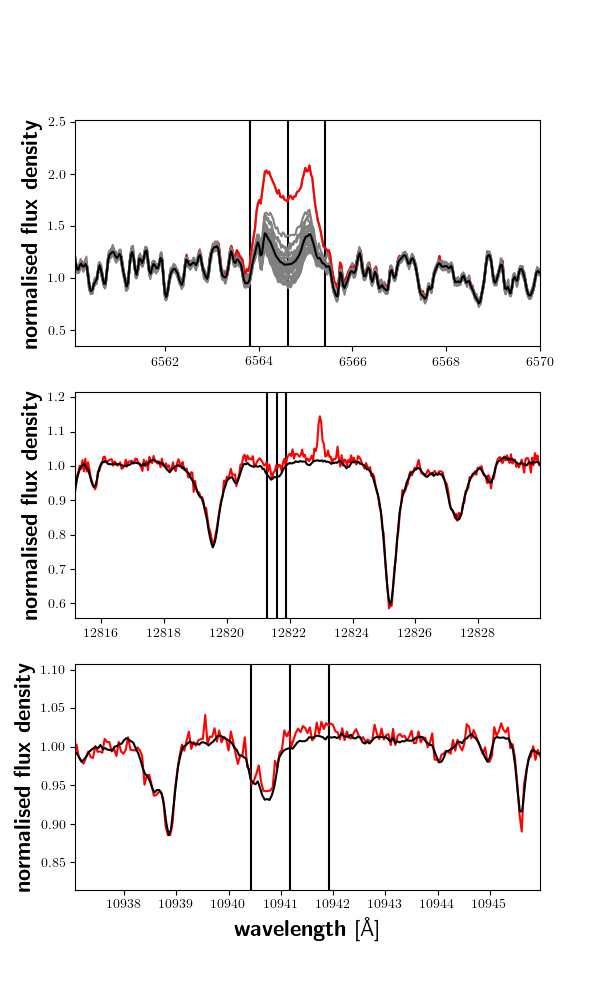
Figure 17: Same as in Fig. 6 but for a Pa$\beta$ flare for the M3.5 V star J02070+496 / G 173-037, which has H$\alpha$ in a transition state between absorption and emission.

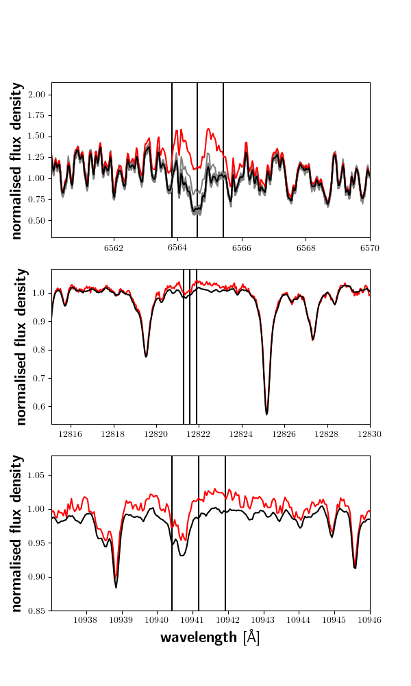
Figure 18: Same as in Fig. 6 but for a Pa$\beta$ flare for the M3.5 V star J11476+786 / GJ 445, which has H$\alpha$ in weak absorption.

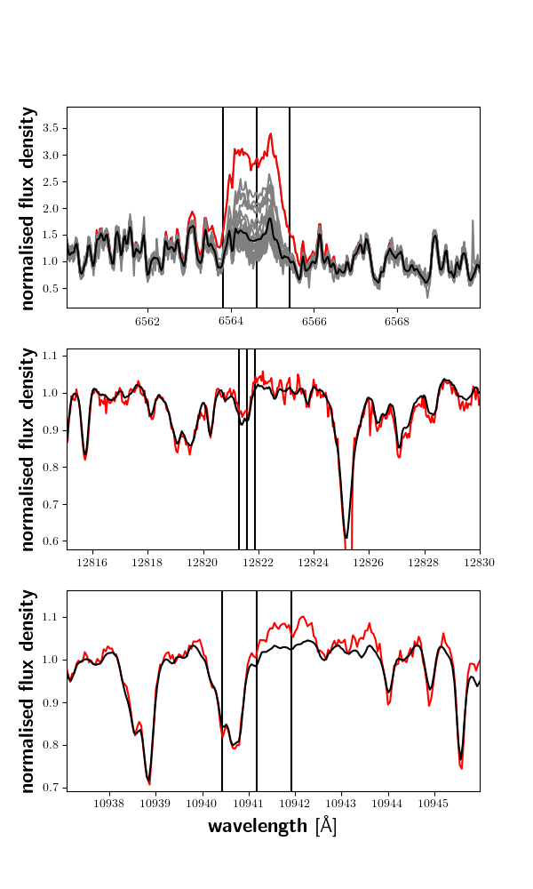
Figure 19: Same as in Fig. 6 but for a Pa$\beta$ flare for the M5.5 V star J23351$-$023 / GJ 1286, which has H$\alpha$ in a transition state between absorption and emission.

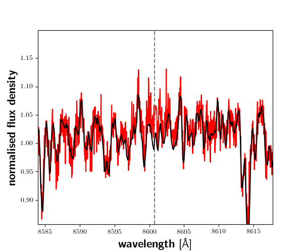
Figure 20: Pa 14 line for the M4.0 V star J13536+776 / RX J1353.6+7737.

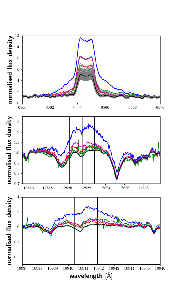
Figure 21: Same as in Fig. 6 but for Pa$\beta$ flares on the M3.5 V J22468+443 / EV Lac. Each coloured spectrum corresponds to one Pa$\beta$ flare. The weakest flare is marked in cyan and has no Pa$\gamma$ emission any more.

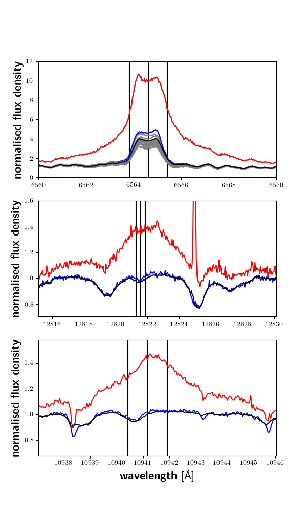
Figure 22: Same as in Fig. 6 but for Pa$\beta$ flares on the M4.0 V star J13536+776 / RX J1353.6+7737. Each coloured spectrum corresponds to one Pa$\beta$ flare.

Appendix C Gaussian fitting of the H$\alpha$ and Pa$\beta$ lines affected by flaring

The fitting parameters of the Gaussian line fitting of the H$\alpha$ and Pa$\beta$ lines, which are affected by flaring, can be found in the Tables 6 and 7 for the automatically and manually found flares, respetively. H$\alpha$ is fitted with a broad and a narrow Gaussian component, while we fit the Pa$\beta$ line with only one Gaussian component as is appropriate for most of the lines. Nevertheless, for some lines no good fit could be established.

Table 6: Gaussian fitting parameters for the H$\alpha$ and Pa$\beta$ line for automatically detected Pa$\beta$ flares.

Karmn	Name	Spec.	JD	$\lambda_{\rm c}$	Area	$\sigma$	$\lambda_{\rm c}$	Area	$\sigma$	$\lambda_{\rm c}$	Area	$\sigma$	log($L_{\mathrm{\mbox{Pa$\beta$}}}/L_{\mathrm{bol}}$)	$\Delta$pEW(Pa$\beta$)	shown in
		type	-2450000
			[day]	[Å]	[Å]	[Å]	[Å]	[Å]	[Å]	[Å]	[Å]	[Å]		[Å]	Fig.
J01019+541	G 218-020	M5.0 V	7761.311	6564.70	7.40	0.59	6565.16	3.1	2.6	12822.1	0.18	1.90	-6.64	0.035
J01033+623	V388 Cas	M5.0 V	7814.315	6563.87	5.66	0.75	6561.48	5.02	1.98	12820.20	0.12	1.05	-5.76	0.017	11
J01125$-$169	YZ Cet	M4.5 V	7959.673	6564.60	1.42	0.60	6565.70	0.55	1.57	…	…	…	…	0.014
J01125$-$169	YZ Cet	M4.5 V	8451.355	6564.61	2.99	0.55	6564.71	0.54	2.00	12821.50	0.12	1.12	-6.02	0.022
J01125$-$169	YZ Cet	M4.5 V	8474.265	6564.61	1.48	0.64	6564.55	2.13	2.81	12821.50	0.12	1.38	-6.02	0.021
J01125$-$169	YZ Cet	M4.5 V	8487.277	6564.63	3.65	0.64	6566.72	0.46	0.84	12821.50	0.10	1.07	-6.10	0.020
J01125$-$169	YZ Cet	M4.5 V	8493.305	6564.59	7.47	0.47	6564.62	2.36	1.71	12821.60	0.20	0.97	-5.80	0.047
J01125$-$169	YZ Cet	M4.5 V	8493.348	6564.60	6.14	0.46	6565.24	2.61	1.56	12821.60	0.09	0.67	-6.14	0.030
J02070+496	G 173-037	M3.5 V	8499.444	6564.62	0.90	0.53	6566.40	0.06	1.4	12822.30	0.17	1.80	-6.44	0.011	17
J07319+362N	BL Lyn	M3.5 V	7449.384	6564.59	2.23	0.73	6565.61	1.49	2.10	12821.60	0.21	1.40	-6.94	0.039	6
J07446+035	YZ CMi	M4.5 V	7788.475	6564.56	2.72	0.89	6564.21	5.00	4.14	12821.60	0.75	3.20	-4.29	0.034
J08298+267	DX Cnc	M6.5 V	9177.625	6564.70	30.0	0.52	6565.07	10.37	1.57	12821.60+	0.39	0.97	-4.03	0.098
J10196+198	AD Leo	M3.0 V	8209.469	6564.62	1.92	0.60	6566.83	0.15	0.92	12821.30	0.07	1.08	-8.16	0.017
J10196+198	AD Leo	M3.0 V	9727.355	6564.63	2.09	0.60	6565.39	0.37	1.88	12821.90	0.19	2.04	-7.73	0.023
J11474+667	1RXS J11472+66a	M5.0 V	7762.546	6564.60	13.58	0.72	6564.33	15.83	3.70	12821.60+	0.95	2.05	-5.99	0.116	13
J11474+667	1RXS J11472+66a	M5.0 V	8852.717	6564.61	22.02	0.75	6565.28	25.0	2.36	12821.60+	2.20	1.90	-5.62	0.278	13
J11476+786	GJ 445	M3.5 V	8845.663	6564.61	0.72	0.64	6564.71	0.58	2.58	12821.80	0.10	2.08	-6.14	0.011	18
J13536+776	RX J1353.6+7737	M4.0 V	8678.409	6564.69	10.28	0.86	6565.03	14.56	3.11	12822.20+	2.14	2.19	-4.25	0.234	22
J13536+776	RX J1353.6+7737	M4.0 V	8877.716*	6564.57	1.17	0.52	…	…	…	…	…	…	…	0.012	22
J15218+209	OT Ser	M1.5 V	7752.704*	6564.64	0.46	1.14	6564.54	1.27	4.08	12821.60	0.15	1.79	-5.09	0.018
J15218+209	OT Ser	M1.5 V	7950.498	6564.62	1.37	0.76	6564.86	1.12	2.37	12821.60	0.39	2.18	-4.69	0.034
J18075$-$159	GJ 1224	M4.5 V	8700.383	6564.62	7.11	0.61	6565.35	1.55	1.96	12821.70	0.38	1.55	-6.10	0.065
J18482+076	G 141-036	M5.0 V	7631.455	6564.55	5.02	0.70	6564.93	3.15	1.94	12821.60	0.18	1.30	-5.81	0.033
J18498$-$238	V1216 Sgr	M3.5 V	8033.285	6564.56	0.70	0.48	…	…	…	…	…	…	…	0.023
J18498$-$238	V1216 Sgr	M3.5 V	8264.646	6564.63	1.02	0.57	6564.66	0.38	1.91	12821.60	0.09	1.58	-6.52	0.020
J18498$-$238	V1216 Sgr	M3.5 V	8300.556	6564.65	4.98	0.56	6564.92	1.70	1.76	12821.60	0.20	1.60	-6.18	0.029
J20451$-$313	AU Mic	M0.5 V	8679.526	6564.67	4.87	1.93	6564.53	5.88	5.78	12821.60	1.73	4.06	-5.13	0.107	14
J20451$-$313	AU Mic	M0.5 V	8679.531	6564.69	2.94	1.60	6564.56	6.31	3.96	12821.60	1.77	4.12	-5.13	0.112	14
J20451$-$313	AU Mic	M0.5 V	8680.522	6564.72	2.53	1.43	6564.41	7.79	3.70	12821.50	2.18	4.48	-5.04	0.040	14
J20451$-$313	AU Mic	M0.5 V	8680.532	6564.91	0.47	0.60	6564.57	1.53	1.49	12821.40	0.12	1.42	-6.30	0.026	14
J20451$-$313	AU Mic	M0.5 V	9161.271*	6564.87	0.46	0.59	6564.61	1.47	1.48	12821.60	0.10	1.18	-6.37	0.040
J22012+283	V374 Peg	M4.0 V	7754.323	6564.24	3.72	0.62	6564.43	1.53	2.65	12820.90	0.22	2.32	-6.06	0.022	10
J22231$-$176	LP 820-012	M4.5 V	7586.616	6564.63	2.30	0.65	6564.98	3.93	1.72	12821.90	0.12	1.34	-6.77	0.026
J22468+443	EV Lac	M3.5 V	7626.537*	6564.59	1.74	0.55	…	…	…	…	…	…	…	0.011
J22468+443	EV Lac	M3.5 V	7632.628	6564.57	2.42	0.72	6563.81	2.35	1.97	12821.60	0.22	1.93	-6.01	0.027	21
J22468+443	EV Lac	M3.5 V	7633.467	6564.61	7.67	0.68	6565.07	9.92	1.75	12821.60	1.16	1.83	-5.29	0.146	21
J22468+443	EV Lac	M3.5 V	7647.373*	6564.72	0.51	0.72	6565.36	1.29	3.35	12821.50	0.10	1.07	-6.35	0.018
J22468+443	EV Lac	M3.5 V	7650.536	6564.59	4.38	0.59	6566.30	2.81	1.67	12821.60	0.10	1.03	-6.35	0.017	21
J22468+443	EV Lac	M3.5 V	7931.662*	6564.63	1.66	0.68	6565.26	0.44	1.84	12821.60	0.18	1.97	-6.10	0.023	21
J22468+443	EV Lac	M3.5 V	8032.429	6564.55	4.98	0.62	6565.20	1.46	1.96	12821.50	0.33	1.27	-5.83	0.054	21
J23351$-$023	GJ 1286	M5.5 V	8080.358	6564.61	2.27	0.57	6563.87	0.41	2.28	12821.70	0.03	0.50	-6.65	0.009	19

Notes: ^∗ Flare detected by eye,^a full designation 1RXS J114728.8+664405,^b full designation 2MASS J07471385+5020386, ⁺ the Pa$\beta$ line is not described well by one Gaussian.

Table 7: Gaussian fitting parameters for the H$\alpha$ and Pa$\beta$ line for visually found Pa$\beta$ flares.

Karmn	Name	Spec.	JD	$\lambda_{\rm c}$	Area	$\sigma$	$\lambda_{\rm c}$	Area	$\sigma$	$\lambda_{\rm c}$	Area	$\sigma$	log($L_{\mathrm{\mbox{Pa$\beta$}}}/L_{\mathrm{bol}}$)	$\Delta$pEW(Pa$\beta$)	shown in
		type	-2450000
			[day]	[Å]	[Å]	[Å]	[Å]	[Å]	[Å]	[Å]	[Å]	[Å]		[Å]	Fig.
J01352$-$072	Barta 161 12	M4.0 V	7735.340	6565.77	4.41	1.64	6567.86	0.85	1.94	12823.60	0.18	2.14	-6.12	0.009	10
J02088+494	G 173-039	M3.5 V	7691.528	6564.99	1.75	0.64	…	…	…	12822.50	0.08	1.32	-5.20	0.009
J02088+494	G 173-039	M3.5 V	7987.588	6564.91	1.16	0.67	6565.25	0.94	1.81	12822.40	0.16	3.34	-4.90	0.012
J03473$-$019	G 80-021	M3.0 V	7677.596	6564.61	0.92	0.57	…	…	…	12821.70	0.06	0.57	-5.54	0.012
J03473$-$019	G 80-021	M3.0 V	7766.314	6564.66	0.81	0.85	…	…	…	…	…	…	…	0.008
J07033+346	LP 255-011	M4.0 V	8857.411	6564.61	1.90	0.61	6564.71	1.97	3.08	12821.60	0.15	1.40	-6.22	0.026
J07472+503	2MASS J0747+502b	M4.0 V	8882.442	…	…	…	…	…	…	…	…	…	…	0.007
J07558+833	GJ 1101	M4.5 V	8041.580	6564.53	1.15	0.64	6564.42	1.19	2.96	12821.60	0.06	0.40	-6.00	0.026	9
J09161+018	RX J0916.1+0153	M4.0 V	7712.658	6564.70	0.99	1.70	6565.64	1.04	5.36	12821.30	0.05	0.81	-6.22	0.031
J11055+435	WX UMa	M5.5 V	9748.384	6564.57	40.00	0.52	6565.54	29.87	1.62	…	…	…	…	0.015
J12156+526	StKM2-809	M4.0 V	7449.654	…	…	…	…	…	…	…	…	…	…	0.005
J12156+526	StKM2-809	M4.0 V	7558.430	…	…	…	…	…	…	…	…	…	…	0.023
J12156+526	StKM2-809	M4.0 V	7752.752	…	…	…	…	…	…	…	…	…	…	0.007
J12428+418	G 123-055	M4.0 V	7754.751	6564.60	2.05	0.58	…	…	…	12821.30	0.07	1.01	-6.65	0.017	16
J16570$-$043	LP 686-027	M3.5 V	7822.700	6564.74	1.72	0.63	6564.10	1.30	1.94	12821.60	0.10	1.07	-7.15	0.018
J22518+317	GT Peg	M3.0 V	7762.276	6564.51	2.23	0.61	6565.89	1.14	1.64	12822.20	0.16	2.46	-5.06	0.011

Notes: ^∗ Flare detected by eye,^a full designation 1RXS J114728.8+664405,^b full designation 2MASS J07471385+5020386