Exceptional set estimate through Brascamp-Lieb inequality

Abstract.

Fix integers $1\leq k<n$, and numbers $a,s$ satisfying $0<s<\min\{k,a\}$. The problem of exceptional set estimate is to determine

$$T(a,s):=\sup_{A\subset\mathbb{R}^{n}\ \textup{dim}A=a}\textup{dim}(\{V\in G(k,n):\textup{dim}(\pi_{V}(A))<s\}).$$

In this paper, we prove a new upper bound for $T(a,s)$ by using Brascamp-Lieb inequality. As one of the corollaries, we obtain the estimate

$$T(a,\frac{k}{n}a)\leq k(n-k)-\min\{k,n-k\},$$

which improves a previous result $T(a,\frac{k}{n}a)\leq k(n-k)-1$ of He.

By constructing examples, we can determine the explicit value of $T(a,s)$ for certain $(a,s)$:

When $k\leq\frac{n}{2}$, $\beta\in(0,1]$ and $\gamma\in(\beta,\frac{k}{n}(1+\beta)]$, we have

$$T(1+\beta,\gamma)=k(n-k)-k.$$

When $k\geq\frac{n}{2}$, $\beta\in(0,1]$ and $\gamma\in(\beta,(1-\frac{k}{n})+\frac{k}{n}\beta]$, we have

$$T(n-1+\beta,k-1+\gamma)=k(n-k)-(n-k).$$

1. Introduction

Let $G(k,n)$ be the set of $m$-dimensional subspaces in $\mathbb{R}^{n}$. For $V\in G(k,n)$, define $\pi_{V}:\mathbb{R}^{n}\rightarrow V$ to be the orthogonal projection onto $V$. Throughout the paper, we use $\dim X$ to denote the Hausdorff dimension of the set $X$.

There is a classical result proved by Marstrand [11], who showed that if $A$ is a Borel set in $\mathbb{R}^{2}$, then the projection of $A$ onto almost every line through the origin has Hausdorff dimension $\min\{1,\dim A\}$. This was generalized to higher dimensions by Mattila [12], who showed that if $A$ is a Borel set in $\mathbb{R}^{n}$, then the projection of $A$ onto almost every $k$-dimensional plane through the origin has Hausdorff dimension $\min\{k,\dim A\}$.

There is a finer question known as the exceptional set estimate. It is formulated as follows. Fix integers $1\leq k<n$. For $a,s$ satisfying $0<s<\min\{k,a\}$, find

(1) $$T(a,s):=\sup_{A\subset\mathbb{R}^{n}\ \textup{dim}A=a}\textup{dim}(\{V\in G(k,n):\textup{dim}(\pi_{V}(A))<s\}).$$

To avoid the measurability issue, we assume the set $A$ is Borel throughout the paper. We remark that $T(a,s)$ also depends on another two parameters $k,n$, but since $k,n$ are fixed, we just drop them from the notation for simplicity.

We call the set

(2) $$E_{s}(A):=\{V\in G(k,n):\textup{dim}(\pi_{V}(A))<s\}$$

the exceptional set. Roughly speaking, the exceptional set is the set of directions where the projection is small. We call $T(a,s)$ the dimension of the exceptional set. Of course, we trivially have $T(a,s)\leq\dim(G(k,n))=k(n-k)$. Here are some nontrivial results on the upper bound of $T(a,s)$.

1. $T(a,s)\leq k(n-k)+s-k$.

2. $T(a,s)\leq\max\{k(n-k)+s-a,0\}.$

3. $T(a,\frac{k}{n}a)\leq k(n-k)-1$.

The estimate (i) was first proved by Kaufman in $\mathbb{R}^{2}$ (see [9]), and proved by Mattila in higher dimensions (see [12]). For the the estimate (ii), it was originally obtained by Falconer (see [3]) in a slightly different formulation. Peres-Schlag also proved the result (see [16]). The estimate (iii) was obtained by He (see [8]). We remark that estimate (iii) beats estimate (i) and (ii) if $k=1,a\in(0,1+\frac{1}{n-1})$ or $k=n-1,a\in(n-1-\frac{1}{n-1},n)$.

In the special case $n=2,k=1$, there were some work by Bourgain [1], Orponen and Shmerkin [15], [14]. Shortly after this paper, this special case was completely resolved by Ren and Wang [17]. They proved that $T(a,s)=\max\{0,2s-a\}$ when $n=2,k=1$.

In this paper, we will explore a new type of the exceptional set estimate, and as one of the result, we can improve (iii).

1.1. Statement of the main result

We fix two integers $1\leq k<n$ throughout this paper. The first theorem is an improvement over the estimate (iii).

Theorem 1.

Suppose $T(a,s)$ is defined in (1). We have

(3) $$T(a,\frac{k}{n}a)\leq k(n-k)-\min\{k,n-k\}.$$

We would like to compare the estimate of $T(a,\frac{k}{n}a)$ given by Theorem 1 with that given by (i) and (ii).

When $k\leq n/2$, Theorem 1 gives $T(a,\frac{k}{n}a)\leq k(n-k)-k$. This automatically beats (i). And it beats (ii) in the range $a\in(0,\frac{nk}{n-k})$.

When $k\geq\frac{n}{2}$, Theorem 1 gives $T(a,\frac{k}{n}a)\leq k(n-k)-(n-k)$. It beats (i) if $a>\frac{(2k-n)n}{k}$, and it beats (ii) if $a<n$. Therefore, it beats both (i) and (ii) in the range $a\in(\frac{(2k-n)n}{k},n)$.

To prove Theorem 1, we will prove a more technical theorem. To handle the numerology, we need to set up some notation.

Lemma 2.

Let $0\leq m\leq n,1\leq k,l\leq n$ be integers. Let $L\in G(l,n)$. We have

$$\dim(\{V\in G(k,n):\dim(\pi_{L}(V))\leq m\})=$$

(7) $$\left\{\begin{array}[]{lr}0&m<\max\{0,l+k-n\}\\ k(n-k)-(k-m)(l-m)&\max\{0,l+k-n\}\leq m\leq\min\{l,k\}\\ k(n-k)&m>\min\{l,k\}\end{array}\right.$$

Proof.

Since $\dim(\pi_{L}(V))\geq\max\{0,l+k-n\}$, we have

$$\dim(\{V\in G(k,n):\dim(\pi_{L}(V))\leq m\})=0$$

for $m<\max\{0,l+k-n\}$.

Since $\dim(\pi_{L}(V))\leq\min\{l,k\}$, we have

$$\dim(\{V\in G(k,n):\dim(\pi_{L}(V))\leq m\})=k(n-k)$$

for $m>\min\{l,k\}$.

It remains to consider the case when $\max\{0,l+k-n\}\leq m\leq\min\{l,k\}$. First by Lemma 35, we have $\dim(\pi_{L}(V))=\dim(\pi_{V}(L))$. We are going to apply Lemma 36 with $W=L$ and the roles of $l$ and $m$ switched. We can verify the conditions of Lemma 36 are satisfied: $n-k\geq l-m$, $m\leq k,l$. Therefore,

(8) $$\dim(\{V\in G(k,n):\dim(\pi_{L}(V))\leq m\})=d(k-m,n-l)+d(m,n-(k-m)).$$

Here, $d(k,n)=k(n-k)$. We can calculate

$$\dim(\{V\in G(k,n):\dim(\pi_{L}(V))\leq m\})=k(n-k)-(k-m)(l-m).$$

∎

Definition 3 (Definition of $E(m,l)$).

We define $E(m,l)$ to be the number in (7). We remark that $E(m,l)$ also depends on $n,k$, but $n,k$ are fixed throughout the paper so we drop them from the notation for simplicity.

Definition 4 (Definition of $m(t,l)$).

For $0\leq t<k(n-k)$ and integer $1\leq l\leq n$, we define $m(t,l)$ to be the smallest non-negative integer so that

$$E(m(t,l),l)>t.$$

By (7), we see $0\leq m(t,l)\leq\min\{l,k\}+1$. We also see that $m(\lfloor t\rfloor,l)=m(t,l)$, since $E(m,l)\in\mathbb{Z}$.

Now, we state our technical theorem.

Theorem 5.

Fix integers $1\leq k<n$. For $0<s<\min\{k,a\}$ and $A\subset\mathbb{R}^{n}$ with $\dim A=a$, define

$$E_{s}(A):=\{V\in G(k,n):\dim(\pi_{V}(A))<s\}.$$

If $s,t$ satisfy

(9) $$s=\sup_{1\leq p\leq\infty}\inf_{l\in\mathbb{Z}\cap[0,n]}\bigg{(}\frac{a-l}{p}+m(t,l)\bigg{)},$$

then

$$\dim(E_{s}(A))\leq t.$$

Remark 6.

The relationship between $s$ and $t$ in (9) has a somewhat weird expression in terms of $\sup$ and $\inf$, because we will apply Brascamp-Lieb inequality during the proof, and the Brascamp-Lieb constant has this form (see (71)).

It seems hard to find an explicit way to express the right hand side of (9) (without using $\sup$, $\inf$). In this paper, we only calculate a special case $s=\frac{k}{n}a$ which gives Theorem 1. It is conceivable that we may obtain some other interesting exceptional set estimates by carefully analyzing (9).

In Section 6, we will find the lower bound of $T(a,s)$ by constructing examples. Together with Theorem 1, we will see for certain range of $(a,s)$, the upper bound and lower bound of $T(a,s)$ are the same, which gives the exact value of $T(a,s)$. This is the following theorem.

Theorem 7.

When $k\leq\frac{n}{2}$, $\beta\in(0,1]$ and $\gamma\in(\beta,\frac{k}{n}(1+\beta)]$, we have

$$T(1+\beta,\gamma)=k(n-k)-k.$$

When $k\geq\frac{n}{2}$, $\beta\in(0,1]$ and $\gamma\in(\beta,(1-\frac{k}{n})+\frac{k}{n}\beta]$, we have

$$T(n-1+\beta,k-1+\gamma)=k(n-k)-(n-k).$$

Remark 8.

From Theorem 7, we see that Theorem 1 is sharp for $a\in(1,2]$ if $k\leq\frac{n}{2}$, and for $a\in(n-1,n]$ if $k\geq\frac{n}{2}$,

Here is the structure of the paper. In Section 2, we prove Theorem 1 using Theorem 5. In Section 3, we give a heuristic proof of Theorem 5. In Section 4 and 5, we prove Theorem 5. In Section 6, we discuss the lower bound of $T(a,s)$ and prove Theorem 7.

Acknowledgement. The author would like to thank Prof. Larry Guth for many helpful discussions. The author would also like to thank referees for useful suggestions.

2. Proof of Theorem 1

Proof of Theorem 1 using Theorem 5.

We set

$$u=\min\{k,n-k\},\ t=k(n-k)-u,\ s=\sup_{1\leq p\leq\infty}\inf_{l\in\mathbb{Z}\cap[0,n]}\bigg{(}\frac{a-l}{p}+m(t,l)\bigg{)}.$$

Theorem 5 implies that

$$T(a,s)\leq t.$$

To prove Theorem 1, it suffices to show

(10) $$\frac{k}{n}a\leq\sup_{1\leq p\leq\infty}\inf_{l\in\mathbb{Z}\cap[0,n]}\bigg{(}\frac{a-l}{p}+m(t,l)\bigg{)}.$$

By choosing $p=\frac{n}{k}$, it is further reduced to

(11) $$\frac{k}{n}a\leq\inf_{l\in\mathbb{Z}\cap[0,n]}\bigg{(}\frac{(a-l)k}{n}+m(t,l)\bigg{)}.$$

By the definition of $u$, we have

(12) $$k\in\{u,n-u\},\ n\geq 2u.$$

We will find an explicit expression for $m(t,l)$. Recall the definition of $m(t,l)$ in Definition 4. $m=m(t,l)$ is the smallest non-negative integer satisfying

$$k(n-k)-(k-m)(l-m)>t,$$

or equivalently,

$$m^{2}-(k+l)m+kl+t-k(n-k)<0.$$

We obtain that

$$m=\sup\{0,\lfloor\frac{k+l-\sqrt{(k-l)^{2}+4(k(n-k)-t)}}{2}\rfloor+1\}.$$

Plugging $t=k(n-k)-u$, we get

(13) $$m=\sup\{0,\lfloor\frac{k+l-\sqrt{(k-l)^{2}+4u}}{2}\rfloor+1\}.$$

To prove (11), we just need to prove for any $0\leq l\leq n$,

$$\frac{k}{n}a\leq\frac{(a-l)k}{n}+\lfloor\frac{k+l-\sqrt{(k-l)^{2}+4u}}{2}\rfloor+1.$$

Equivalently,

(14) $$\frac{lk}{n}\leq\lfloor\frac{k+l-\sqrt{(k-l)^{2}+4u}}{2}\rfloor+1.$$

We discuss two cases.

Case 1: $0\leq l\leq k$ We write $l=k-\mu$ with $\mu\geq 0$. Then the right hand side of (14) is

$$\lfloor\frac{-\mu-\sqrt{\mu^{2}+4u}}{2}\rfloor+k+1.$$

Let $\alpha$ be the biggest integer such that $\alpha<\frac{\mu+\sqrt{\mu^{2}+4u}}{2}$, or in other words, $\alpha=-\lfloor\frac{-\mu-\sqrt{\mu^{2}+4u}}{2}\rfloor-1$. Then (14) boils down to

(15) $$(k-\mu)k\leq n(k-\alpha).$$

There are two subcases.

When $u\leq\mu$, then $\alpha<\frac{\mu+\sqrt{\mu^{2}+4u}}{2}\leq\frac{2\mu+2}{2}$, so $\alpha\leq\mu$. We see (15) holds since $n>k$.

When $u\geq\mu+1$, we just need to verify (15) at two endpoints $k=u,k=n-u$. For $k=u$, (15) becomes $(u-\mu)u\leq n(u-\alpha)$. Using the bound $n\geq 2u$, we just need to show $u+\mu\geq 2\alpha$. Noting $\mu^{2}+4u\leq(u+1)^{2}$, we have $\alpha<\frac{\mu+u+1}{2}$, and hence $\alpha\leq\frac{\mu+u}{2}$. For $k=n-u$, (15) becomes $(n-u-\mu)(n-u)\leq n(n-u-\alpha)$, which is equivalent to $u(u+\mu)\leq n(u+\mu-\alpha)$. Using the bound $n\geq 2u$, it boils down to $u+\mu\geq 2\alpha$ which has been proved.

Case 2: $k\leq l\leq n$ We write $l=k+\mu$ with $\mu\geq 0$. Then the right hand side of (14) is

$$\lfloor\frac{\mu-\sqrt{\mu^{2}+4u}}{2}\rfloor+k+1.$$

Let $\alpha$ be the biggest integer such that $\alpha<\frac{\sqrt{\mu^{2}+4u}-\mu}{2}$, or in other words, $\alpha=-\lfloor\frac{\mu-\sqrt{\mu^{2}+4u}}{2}\rfloor-1$. Then (14) boils down to

(16) $$(k+\mu)k\leq n(k-\alpha).$$

There are two subcases.

When $u\leq\mu$, then $\alpha<\frac{\sqrt{\mu^{2}+4u}-\mu}{2}\leq\frac{\mu+2-\mu}{2}$, so $\alpha\leq 0$. We see (16) holds since $n\geq l=k+\mu$.

When $u\geq\mu+1$, we just need to verify (16) at two endpoints $k=u,k=n-u$. For $k=u$, (16) becomes $(u+\mu)u\leq n(u-\alpha)$. Using the bound $n\geq 2u$, we just need to show $u-\mu\geq 2\alpha$. Noting $\mu^{2}+4u\leq(u+1)^{2}$, we have $\alpha<\frac{u+1-\mu}{2}$, and hence $\alpha\leq\frac{u-\mu}{2}$. For $k=n-u$, (16) becomes $(n-u+\mu)(n-u)\leq n(n-u-\alpha)$, which is equivalent to $u(u-\mu)\leq n(u-\mu-\alpha)$. Using the bound $n\geq 2u$, it boils down to $u-\mu\geq 2\alpha$ which has been proved.

∎

3. A heuristic proof of Theorem 5

The main idea in the proof of Theorem 5 is as follows. Suppose there is a set $A$ satisfying the condition in Theorem 5 such that

$$\dim(E_{s}(A))=\tau>t,$$

then we will derive a contradiction.

We consider the following heuristic setting. $A$ is a disjoint union of $\delta$-balls with cardinality $\delta^{-a}$. Our exceptional set $E$ is a $\delta$-separated subset of $G(k,n)$ with cardinality $\delta^{-\tau}$. We also assume $E$ satisfies the $(\delta,\tau)$-condition:

(17) $$\#(E\cap Q_{r})\leq(r/\delta)^{\tau},$$

for any $Q_{r}\subset G(k,n)$ being a ball of radius $r$. The condition that $\dim(\pi_{V}(A))<s$ is characterized in the following way. For each $V\in E$, we have a set of $(n-k)$-dimensional $\delta$-slabs $\mathbb{T}_{V}=\{T\}$ orthogonal to $V$. In other words, each $T\in\mathbb{T}_{V}$ is a rectangle of dimensions $\delta\times\dots\times\delta\times 1\times\dots\times 1$ (with $n-k$ many $1$’s), and the longest $n-k$ directions are orthogonal to $V$. We also assume $A\subset\bigcup_{T\in\mathbb{T}_{V}}T$ and $\#\mathbb{T}_{V}\leq\delta^{-s+\varepsilon_{0}}$. Under these conditions, one is able to deduce some relationships among the parameters $n,k,a,s,t$. We consider the integral

(18) $$\int_{A}(\sum_{V\in E}\sum_{T\in\mathbb{T}_{V}}1_{T})^{p},$$

where $1\leq p\leq\infty$ is to be determined later. Since $A\subset\bigcup_{T\in\mathbb{T}_{V}}T$, a straightforward observation gives

$$\int_{A}(\sum_{V\in E}\sum_{T\in\mathbb{T}_{V}}1_{T})^{p}\sim|A|(\#E)^{p}\sim\delta^{n-a-\tau p}.$$

On the other hand, we will also obtain an upper bound for the integral. Obtaining an upper bound for the integral is more complicated. Let us first take a look at a single $\delta$-ball $B_{\delta}\subset A$. By our assumption, for each $V\in E$, there is a $T\in\mathbb{T}_{V}$ such that $T\cap B_{\delta}\neq\emptyset$. Let $K$ be a scale such that $\delta\ll K^{-1}\ll 1$, and we partition $G(k,n)$ into $K^{-1}$-balls $\mathcal{Q}=\{Q\}$ (here $K^{-1}$-ball means ball of radius $K^{-1}$). Denote the number $J=\lfloor K^{\tau}/2\rfloor$. The key observation is the following inequality.

(19) $$\delta^{-\tau}=\#E\lesssim K^{O(1)}\sum_{Q_{1},\dots,Q_{J}\in\mathcal{Q}}\bigg{(}\prod_{j=1}^{J}\#(Q_{j}\cap E)\bigg{)}^{1/J}.$$

Here, $Q_{1},\dots,Q_{J}$ are different.

We give a proof for (19). Label the balls $Q_{1},Q_{2},\dots,Q_{J},\dots$ in $\mathcal{Q}$ so that $\#(Q_{1}\cap E)\geq\#(Q_{2}\cap E)\geq\dots\geq\#(Q_{J}\cap E)\geq\dots$. We just need to prove $\#(Q_{J}\cap E)\gtrsim K^{-O(1)}\#E$. By (17), $\sum_{j=1}^{J}\#(Q_{j}\cap E)\leq J/(K\delta)^{\tau}\leq\#E/2$. Therefore,

$$\#(Q_{J}\cap E)\geq\frac{1}{\#\mathcal{Q}}\sum_{j\geq J+1}\#(Q_{j}\cap E)\geq\frac{1}{\#\mathcal{Q}}\#E/2\gtrsim K^{-O(1)}\#E.$$

By (19), we can bound the integral (18) by the multilinear form

(20) $$\int_{A}(\sum_{V\in E}\sum_{T\in\mathbb{T}_{V}}1_{T})^{p}\lesssim K^{O(1)}\sum_{Q_{1},\dots,Q_{J}\in\mathcal{Q}}\int\prod_{j=1}^{J}\bigg{(}\sum_{V\in Q_{j}\cap E}\sum_{T\in\mathbb{T}_{V}}1_{T}\bigg{)}^{p/J}.$$

The transversality property of these $J$ patches allows us to obtain a nice upper bound. The main tool we use to handle this $J$-linear integral is the Brascamp-Lieb inequality. In the end, we will check the numerology and see the contradiction if $\tau>t$.

Let us work on a very easy case when $n=2,k=1$. We give a heuristic proof for the estimate

$$\dim(E_{a/2}(A))=0.$$

We just follow the argument as above. We will choose $p=2$.

Suppose by contradiction that $\dim(E_{a/2}(A))>0$. Then there exists $\varepsilon_{0}>0$ such that $\dim(E_{a/2-\varepsilon_{0}}(A))=\tau>0$. On the one hand,

$$\int_{A}(\sum_{V\in E}\sum_{T\in\mathbb{T}_{V}}1_{T})^{2}\sim\delta^{2-a-2\tau}.$$

For the upper bound, we notice that $J=\lfloor K^{\tau}/2\rfloor\geq 2$ (if $K$ is large), so we could just use the bilinear integral as an upper bound:

$$\int_{A}(\sum_{V\in E}\sum_{T\in\mathbb{T}_{V}}1_{T})^{2}\lesssim\int\bigg{(}\sum_{V\in Q_{1}\cap E}\sum_{T\in\mathbb{T}_{V}}1_{T}\bigg{)}\bigg{(}\sum_{V\in Q_{2}\cap E}\sum_{T\in\mathbb{T}_{V}}1_{T}\bigg{)}\lesssim\delta^{2}(\#E\delta^{-a/2+\varepsilon_{0}})^{2},$$

where $Q_{1},Q_{2}$ are two arcs of $S^{1}$ with distance $\sim 1$ from each other. Note that $\#E=\delta^{-\tau}$. Combining the two estimates gives $1\lesssim\delta^{2\varepsilon_{0}}$ which is a contradiction.

For the proof of general $n$ and $k$, our argument is similar. The full details will be given in the next section.

4. The proof of Theorem 5

4.1. Preliminary

We recall some properties of affine Grassmannians from [5, Section 1.2].

Let $G(k,n)$ be the set of $k$-dimensional subspaces in $\mathbb{R}^{n}$. For every $k$-plane $V$, we can uniquely write it as

$$V=\textup{dir}(V)+x_{V},$$

where $\textup{dir}(V)\in G(k,n)$ and $x_{V}\in V^{\perp}$. $\textup{dir}(V)$ refers to the direction of $V$, as can be seen that $\textup{dir}(V)=\textup{dir}(V^{\prime})\Leftrightarrow V\parallel V^{\prime}$.

In this paper, we use $A(k,n)$ to denote the set of $k$-planes $V$ such that $x_{V}\in B^{n}(0,1/2)$. ($B^{n}(0,1/2)$ is the ball of radius $1/2$ centered at the origin in $\mathbb{R}^{n}$.)

$$A(k,n)=\{V:V\textup{~{}is~{}a~{}}k\textup{~{}dimensional~{}plane~{}},x_{V}\in B^{n}(0,1/2)\}.$$

Usually $A(k,n)$ denotes all the $k$-planes in other references, but for our purpose we only care about those $V$ that lie near the origin.

Next, we discuss the metrics on $G(k,n)$ and $A(k,n)$. For $V_{1},V_{2}\in G(k,n)$, we define

$$d(V_{1},V_{2})=\|\pi_{V_{1}}-\pi_{V_{2}}\|.$$

Here, $\pi_{V_{1}}:\mathbb{R}^{n}\rightarrow V_{1}$ is the orthogonal projection. We have another characterization for this metric. Define $\rho(V_{1},V_{2})$ to be the smallest number $\rho$ such that $B^{n}(0,1)\cap V_{1}\subset N_{\rho}(V_{2})$. We have the comparability of $d(\cdot,\cdot)$ and $\rho(\cdot,\cdot)$.

Lemma 9.

There exists a constant $C>0$ (depending on $k,n$) such that

$$\rho(V_{1},V_{2})\leq d(V_{1},V_{2})\leq C\rho(V_{1},V_{2}).$$

Proof.

Suppose $B^{n}(0,1)\cap V_{1}\subset N_{\rho}(V_{2})$, then for any $v\in\mathbb{R}^{n}$, we have

$$|\pi_{V_{1}}(v)-\pi_{V_{2}}(v)|\lesssim\rho|v|,$$

which implies $d(V_{1},V_{2})\lesssim\rho$. On the other hand, if for any $|v|\leq 1$ we have

$$|\pi_{V_{1}}(v)-\pi_{V_{2}}(v)|\leq d|v|,$$

then we obtain that $\pi_{V_{1}}(v)\subset N_{d}(V_{2})$. Letting $v$ ranging over $B^{n}(0,1)\cap V_{1}$, we get $B^{n}(0,1)\cap V_{1}\subset N_{d}(V_{2})$, which means $\rho(V_{1},V_{2})\leq d$. ∎

We can also define the metric on $A(k,n)$ given by

(21) $$d(V,V^{\prime})=d(\textup{dir}(V),\textup{dir}(V^{\prime}))+|x_{V}-x_{V^{\prime}}|.$$

Here, we still use $d$ to denote the metric on $A(k,n)$ and it will not make any confusion.

Similarly, for $V,V^{\prime}\in A(k,n)$ we can define $\rho(V,V^{\prime})$ to be the smallest number $\rho$ such that $B^{n}(0,1)\cap V\subset N_{\rho}(V^{\prime})$. We also have the following lemma. We left the proof to the interested readers.

Lemma 10.

There exists a constant $C>0$ (depending on $k,n$) such that for $V,V^{\prime}\in A(k,n)$,

$$C^{-1}d(V,V^{\prime})\leq\rho(V,V^{\prime})\leq Cd(V,V^{\prime}).$$

Definition 11.

For $V\in A(k,n)$ and $0<r<1$, we define

$$V_{r}:=N_{r}(V)\cap B^{n}(0,1).$$

We see that $V_{r}$ is morally a slab of dimensions $\underbrace{r\times\dots\times r}_{n-k\textup{~{}times}}\times\underbrace{1\times\dots\times 1}_{k\textup{~{}times}}$. We usually call $V_{r}$ a $k$-dimensional $r$-slab. When $k$ is already clear, we simply call $V_{r}$ an $r$-slab. If $W$ is a convex set such that $C^{-1}W\subset V_{r}\subset CW$, then we also call $W$ an $r$-slab. Here, the constant $C$ will be a fixed large constant.

Definition 12.

We say two $r$-slabs $V_{r}$ and $V^{\prime}_{r}$ are comparable if $C^{-1}V_{r}\subset V^{\prime}_{r}\subset CV_{r}$. We say they are essentially distinct if they are not comparable.

In this paper, we will also consider the balls and $\delta$-neighborhood in $A(k,n)$. Recall that we use $B_{r}(x)$ to denote the ball in $\mathbb{R}^{n}$ of radius $r$ centered at $x$. To distinguish the ambient space, we will use letter $Q$ to denote the balls in $A(k,n)$. For $V\in A(k,n)$, we use $Q_{r}(V)$ to denote the ball in $A(k,n)$ of radius $r$ centered at $V$. More precisely,

$$Q_{r}(V_{0}):=\{V\in A(k,n):d(V,V_{0})\leq r\}.$$

For a subset $X\subset A(k,n)$, we use the fancy letter $\mathcal{N}$ to denote the neighborhood in $A(k,n)$:

$$\mathcal{N}_{r}(X):=\{V\in A(k,n):d(V,X)\leq r\}.$$

Here, $d(V,X)=\inf_{V^{\prime}\in X}d(V,V^{\prime})$.

Next, we briefly recall how to define the Hausdorff dimension for subsets of a metric space. Let $(M,d)$ be a metric space. For $X\subset M$, we denote the $s$-dimensional Hausdorff measure of $X$ under the metric $d$ to be $\mathcal{H}^{s}(X;d)$. We see that if $d^{\prime}$ is another metric on $M$ such that $d(\cdot,\cdot)\sim d^{\prime}(\cdot,\cdot)$, then $\mathcal{H}^{s}(X;d)\sim\mathcal{H}^{s}(X;d^{\prime})$. It make sense to define the Hausdorff dimension of $X$ which is independent of the choice of comparable metrics:

$$\dim X:=\sup\{s:\mathcal{H}^{s}(X;d)>0\}.$$

4.2. $\delta$-discretization

Definition 13.

For a number $\delta>0$ and any set $X$ (in a metric space), we use $|X|_{\delta}$ to denote the maximal number of $\delta$-separated points in $X$.

Definition 14 ($(\delta,s)$-set).

Let $\delta,s>0$. For $A\subset\mathbb{R}^{n}$, we say $A$ is a $(\delta,s,C)$-set if $A$ is $\delta$-separated and satisfies the following estimate:

$$\#(A\cap B_{r}(x))\leq C(r/\delta)^{s}$$

for any $x\in\mathbb{R}^{n}$ and $r\geq\delta$. For the purpose of this paper, the constant $C$ is not important, so we simply say $A$ is a $(\delta,s)$-set if it satisfies

$$\#(A\cap B_{r}(x))\lesssim(r/\delta)^{s}.$$

Remark 15.

Throughout the rest of this paper, We will use $\#E$ to denote the cardinality of a set $E$ and $\lvert\cdot\rvert$ to denote the measure of a region.

We state two lemmas:

Lemma 16.

Let $\delta,s>0$ and let $B\subset\mathbb{R}^{n}$ be any set with $\mathcal{H}^{s}_{\infty}(B)=:\kappa>0$. Then, there exists a $(\delta,s)$-set $P\subset B$ with $\#P\gtrsim\kappa\delta^{-s}$.

Proof.

See [4] Lemma 3.13. ∎

Lemma 17.

Fix $a>0$. Let $\nu$ be a probability measure satisfying $\nu(B_{r})\leq Cr^{a}$ for any $B_{r}$ being a ball of radius $r$. If $A$ is a set satisfying $\nu(A)\geq\kappa$ ($\kappa>0$), then for any $\delta>0$ there exists a subset $F\subset A$ such that $F$ is a $(\delta,a)$-set and $\#F\gtrsim\kappa C^{-1}\delta^{-a}$.

Proof.

By the previous lemma, we just need to show $\mathcal{H}^{a}_{\infty}(A)\gtrsim\kappa C^{-1}$. We just check it by definition. For any covering $\{B\}$ of $A$, we have

$$\kappa\leq\sum_{B}\nu(B)\leq C\sum_{B}r(B)^{a}.$$

Ranging over all the covering of $A$ and taking infimum, we get

$$\kappa C^{-1}\lesssim\mathcal{H}^{a}_{\infty}(A).$$

∎

A key step in the proof of Theorem 5 is the following estimate.

Proposition 18.

Let $0<\tau\leq k(n-k),0<\sigma\leq k$. For any $\gamma\in(0,\frac{1}{10})$, there exists $\delta_{0}(\gamma)>0$ depending on $\gamma$ such that for any $\delta<\delta_{0}(\gamma)$, the following is true.

Suppose $E\subset G(k,n)$ is a $(\delta,\tau)$-set with $\#E\gtrsim|\log\delta|^{-2}\delta^{-\tau}$. Suppose for any $V\in E$, there is a set of $(n-k)$-dimensional $\delta$-slabs $\mathbb{T}_{V}$. Each $T\in\mathbb{T}_{V}$ lies in $B^{n}(0,1)$ which has dimensions

$$\underbrace{\delta\times\delta\times\dots\times\delta}_{k\text{~{}times}}\times\underbrace{1\times 1\times\dots\times 1}_{n-k\text{~{}times}}$$

such that the $1\times\dots\times 1$-side is orthogonal to $V$, and

(22) $$\#\mathbb{T}_{V}\leq\delta^{-\sigma}.$$

Let $W=\sqcup B_{\delta}\subset B^{n}(0,1)$ be a disjoint union of $\delta$-balls such that for any $B_{\delta}\subset W$,

(23) $$\#\bigg{\{}V\in E:B_{\delta}\cap\bigcup_{T\in\mathbb{T}_{V}}T\neq\emptyset\bigg{\}}\geq|\log\delta|^{-3}\#E.$$

For $1\leq p<\infty$, set $\lambda_{p}:=\sup_{l\in\mathbb{Z}\cap[0,n]}(l-p\cdot m(t,l))$ (recalling $m(t,l)$ in Definition (4)). We have

(24) $$\int_{W}\Big{(}\sum_{V\in E}\sum_{T\in\mathbb{T}_{V}}1_{T}\Big{)}^{p}\leq C_{\gamma,p}\delta^{-\gamma}\delta^{n}\delta^{-\lambda_{p}}(\delta^{-\sigma-\tau})^{p}.$$

We will prove Theorem 5 assuming Proposition 18, and then come back to the proof of Proposition 18. Before starting the proof, we state a very useful lemma. We use the following notation. Fix a dimension $m$. For any $\delta=2^{-k}$ ($k\in\mathbb{N}^{+}$), let $\mathcal{D}_{\delta}$ denote the lattice $\delta$-cubes in $[0,1]^{m}$.

Lemma 19.

Suppose $X\subset[0,1]^{m}$ with $\dim X<s$. Then for any $\varepsilon>0$, there exist dyadic cubes $\mathcal{C}_{2^{-k}}\subset\mathcal{D}_{2^{-k}}$ $(k>0)$ so that

1. $X\subset\bigcup_{k>0}\bigcup_{D\in\mathcal{C}_{2^{-k}}}D,$

2. $\sum_{k>0}\sum_{D\in\mathcal{C}_{2^{-k}}}r(D)^{s}\leq\varepsilon$,

3. $\mathcal{C}_{2^{-k}}$ satisfies the $s$-dimensional condition: For $l<k$ and any $D\in\mathcal{D}_{2^{-l}}$, we have $\#\{D^{\prime}\in\mathcal{C}_{2^{-k}}:D^{\prime}\subset D\}\leq 2^{(k-l)s}$.

Proof.

See [6] Lemma 2. ∎

Remark 20.

Besides $[0,1]^{m}$, this Lemma also works for other compact metric spaces, for example $\mathbb{S}^{m}$ and $G(k,m)$, which we will use throughout the rest of the paper.

Proof of Theorem 5.

Fix $p\in[1,\infty)$. Let $s$ be given by

$$s=\inf_{l\in\mathbb{Z}\cap[0,n]}\bigg{(}\frac{a-l}{p}+m(t,l)\bigg{)}.$$

Our goal is to prove

(25) $$\dim(E_{s}(A))\leq t.$$

If this is true, then we also obtain (25) for

$$s=\sup_{1\leq p\leq\infty}\inf_{l\in\mathbb{Z}\cap[0,n]}\bigg{(}\frac{a-l}{p}+m(t,l)\bigg{)}$$

by a limiting argument.

By a standard argument, we may assume $A\subset B^{n}(0,1)$. We will do a series of reductions. Noting that

$$E_{s}(A)=\bigcup_{\sigma<s,\sigma\in\mathbb{Q}}E_{\sigma}(A)$$

which is a countable union, we just need to prove

(26) $$\dim(E_{\sigma}(A))\leq t$$

for any $\sigma<s$.

We choose $\alpha<\dim(A),\tau<\dim(E_{\sigma}(A))$. By Frostman’s lemma there exists a probability measure $\nu_{A}$ supported on $A$ satisfying $\nu_{A}(B_{r})\leq C_{A,\alpha}r^{\alpha}$ for any $B_{r}$ being a ball of radius $r$. There exists a probability measure $\nu_{E}$ supported on $E_{\sigma}(A)\subset G(k,n)$ satisfying $\nu_{E}(Q_{r})\leq C_{E_{\sigma}(A),\tau}r^{\tau}$ for any $Q_{r}$ being a ball of radius $r$ in $G(k,n)$. Since our sets $A,E_{\sigma}(A)$, and numbers $\alpha,\tau$ are fixed, we may simply write the Frostman’s condition as

(27) $$\nu_{A}(B_{r})\lesssim r^{\alpha},\ \ \nu_{E}(Q_{r})\lesssim r^{\tau}.$$

Here the implicit constants depend on $A,E_{\sigma}(A),\alpha,\tau$. We will later introduce two scales $0<\delta\ll K^{-1}\ll 1$, and what important here is that the implicit constants never depend on $K^{-1},\delta$.

We only need to prove

$$\tau\leq t,$$

as we can send $\tau\rightarrow\dim(E_{\sigma}(A))$, which gives (26). If this is not true, then there exists $\varepsilon_{1}>0$ such that

(28) $$\tau>2\varepsilon_{1}+t.$$

We may make $\varepsilon_{1}$ smaller so that

(29) $$s>2\varepsilon_{1}+\sigma.$$

We will derive a contradiction.

Now we start the $\delta$-discretization. Fix a $V\in E_{\sigma}(A)$. By definition, we have $\dim(\pi_{V}(A))<\sigma$. We also fix a small number $\epsilon_{\circ}$ which we will later send to $0$. By Lemma 19, we can find a covering of $\pi_{V}(A)$ by dyadic cubes $\mathbb{D}_{V}=\{D\}$, each of which has side-length $2^{-j}$ for some integer $j>|\log_{2}\epsilon_{\circ}|$. $\mathbb{D}_{V}$ also satisfies the following property. Define $\mathbb{D}_{V,j}:=\{D\in\mathbb{D}_{V}:r(D)=2^{-j}\}$. Then we have:

(30) $$\sum_{D\in\mathbb{D}_{V}}r(D)^{s}<1,$$

and for each $j$ and $r$-ball $B_{r}\subset V$, we have

(31) $$\#\{D\in\mathbb{D}_{V,j}:D\subset B_{r}\}\leq\left(\frac{r}{2^{-j}}\right)^{\sigma}.$$

After finding such a $\mathbb{D}_{V}$, we can define a set of $\delta$-slabs by lifting $\mathbb{D}_{V}$ using the map $\pi_{V}$. More precisely, we define the set of slabs $\mathbb{T}_{V,j}:=\{\pi^{-1}_{V}(D):D\in\mathbb{D}_{V,j}\}\cap B^{n}(0,2)$, $\mathbb{T}_{V}=\bigcup_{j}\mathbb{T}_{V,j}$. Each slab in $\mathbb{T}_{V,j}$ roughly has dimensions

$$\underbrace{2^{-j}\times 2^{-j}\times\dots\times 2^{-j}}_{k\text{~{}times}}\times\underbrace{1\times 1\times\dots\times 1}_{n-k\text{~{}times}}$$

such that the $1\times\dots\times 1$-side is orthogonal to $V$. We will use $T$ to denote the slabs in $\mathbb{T}_{V,j}$. One easily sees that $A\subset\bigcup_{T\in\mathbb{T}_{V}}T$. By pigeonholing, there exists an integer $j(V)>|\log_{2}\epsilon_{\circ}|$ such that

(32) $$\nu_{A}(A\cap(\bigcup_{T\in\mathbb{T}_{V,j(V)}}T))\geq\frac{1}{10j(V)^{2}}\nu_{A}(A)=\frac{1}{10j(V)^{2}}.$$

For each $j>|\log_{2}\epsilon_{\circ}|$, define $E_{\sigma,j}(A):=\{V\in E_{\sigma}(A):j(V)=j\}$. Then we obtain a partition of $E_{\sigma}(A)$:

$$E_{\sigma}(A)=\bigsqcup_{j}E_{\sigma,j}(A).$$

By pigeonholing again, there exists $j$ such that

(33) $$\nu_{E}(E_{\sigma,j}(A))\geq\frac{1}{10j^{2}}.$$

In the rest of the proof, we fix this $j$. We also set $\delta=2^{-j}$. We remark that $\delta\leq\epsilon_{\circ}$. Therefore, we can make $\delta\rightarrow 0$ by letting $\epsilon_{\circ}\rightarrow 0$.

By Lemma 17, there exists a $(\delta,\tau)$-set $E\subset E_{\sigma,j}(A)$ with cardinality

(34) $$\#E\gtrsim|\log\delta|^{-2}\delta^{-\tau}.$$

Next, we consider the set $S:=\{(x,V)\in A\times E:x\in\bigcup_{T\in\mathbb{T}_{V,j}}T\}$. We also use $\mu$ to denote the counting measure on $E$. Define the sections of $S$:

$$S_{x}=\{V\in E:(x,V)\in S\},\ \ \ S_{V}:=\{x\in A:(x,V)\in S\}.$$

By (32) and Fubini, we have

(35) $$(\nu_{A}\times\mu)(S)=\sum_{V\in E}\nu_{A}(S_{V})\geq\frac{1}{10j^{2}}\#E.$$

This implies

(36) $$(\nu_{A}\times\mu)\bigg{(}\Big{\{}(x,V)\in S:\mu(S_{x})\geq\frac{1}{20j^{2}}\#E\Big{\}}\bigg{)}\geq\frac{1}{20j^{2}}\#E,$$

since

(37) $$(\nu_{A}\times\mu)\bigg{(}\Big{\{}(x,V)\in S:\mu(S_{x})\leq\frac{1}{20j^{2}}\#E\Big{\}}\bigg{)}\leq\frac{1}{20j^{2}}\#E.$$

By (36), we have

(38) $$\nu_{A}\bigg{(}\Big{\{}x\in A:\mu(S_{x})\geq\frac{1}{20j^{2}}\#E\Big{\}}\bigg{)}\geq\frac{1}{20j^{2}}.$$

Recall $\delta=2^{-j}$. By (38) and Lemma 17, we can find a $\delta$-separated set $H\subset\{x\in A:\#S_{x}\geq\frac{1}{20j^{2}}\#E\}$ with cardinality

(39) $$\#H\gtrsim|\log\delta|^{-2}\delta^{-\alpha}.$$

For simplicity, we will omit the subscript $j$ and use $\mathbb{T}_{V}$ to denote $\mathbb{T}_{V,j}$ which is a set of $(n-k)$-dimensional $\delta$-slabs that are orthogonal to $V$. Also by (31),

(40) $$\#\mathbb{T}_{V}\leq\delta^{-\sigma}.$$

Now we focus on the estimate of the integral

$$\int_{N_{\delta}(H)}\Big{(}\sum_{V\in E}\sum_{T\in\mathbb{T}_{V}}1_{T}\Big{)}^{p}.$$

The lower bound is easy. By the definition of $H$, we see that for any $x\in H$, there are $\gtrsim|\log\delta|^{-2}\#E$ many slabs from $\cup_{V\in E}\mathbb{T}_{V}$ that intersect $x$. In other words,

$$\sum_{V\in E}\sum_{T\in\mathbb{T}_{V}}1_{T}(x)\gtrsim|\log\delta|^{-2}\#E.$$

Therefore, we get the lower bound

(41) $$\int_{N_{\delta}(H)}\Big{(}\sum_{V\in E}\sum_{T\in\mathbb{T}_{V}}1_{T}\Big{)}^{p}\gtrsim|\log\delta|^{-2p}\delta^{n}\#H\#E^{p}.$$

Next, we use Proposition 18 to obtain an upper bound. Noting that $H$ is $\delta$-separated, $N_{\delta}(H)$ is a disjoint union of $\delta$-balls. We let the $W$ in Proposition 18 to be $N_{\delta}(H)$. We can also check the other conditions in Proposition 18 are satisfied. Therefore, we obtain

(42) $$\int_{N_{\delta}(H)}\Big{(}\sum_{V\in E}\sum_{T\in\mathbb{T}_{V}}1_{T}\Big{)}^{p}\leq C_{\gamma,p}\delta^{-\gamma}\delta^{n}\delta^{-\lambda_{p}}(\delta^{-\sigma-\tau})^{p}.$$

Comparing with the lower bound (41), we obtain

(43) $$\delta^{n}\delta^{-\alpha}\delta^{-\tau p}\lesssim_{\gamma,p}\delta^{-\gamma}|\log\delta|^{O(1)}\delta^{n}\delta^{-\lambda_{p}}(\delta^{-\sigma-\tau})^{p},$$

where $\lambda_{p}=\sup_{l\in\mathbb{Z}\cap[0,n]}(l-p\cdot m(t,l)).$ Letting $\delta\rightarrow 0$ and then $\gamma\rightarrow 0$ gives that

(44) $$\sigma\geq\frac{\alpha-\lambda_{p}}{p}.$$

On the other hand, by our choice of $\sigma$,

(45) $$\sigma<s-2\varepsilon_{1}=\inf_{l\in\mathbb{Z}\cap[0,n]}(\frac{a-l}{p}+m(t,l))-2\varepsilon_{1}.$$

Combining with (44), we obtain

(46) $$\inf_{l\in\mathbb{Z}\cap[0,n]}(\frac{\alpha-l}{p}+m(t,l))<\inf_{l\in\mathbb{Z}\cap[0,n]}(\frac{a-l}{p}+m(t,l))-2\varepsilon_{1}.$$

This gives a contradiction by letting $\alpha\rightarrow a$.

∎

5. Proof of Proposition 18

We have

(47) $$\int_{W}\Big{(}\sum_{V\in E}\sum_{T\in\mathbb{T}_{V}}1_{T}\Big{)}^{p}\lesssim\delta^{n}\sum_{B_{\delta}\subset W}\#\{T\in\cup_{V\in E}\mathbb{T}_{V}:B_{\delta}\cap T\neq\emptyset\}^{p}.$$

For $B_{\delta}\subset W$, we define the set

(48) $$E(B_{\delta}):=\{V\in E:B_{\delta}\cap\bigcap_{T\in\mathbb{T}_{V}}T\neq\emptyset\}.$$

Since for each $B_{\delta}$ and $V\in E$, there are $\lesssim 1$ tubes in $\mathbb{T}_{V}$ that intersect $B_{\delta}$, we have

$$\#\{T\in\cup_{V\in E}\mathbb{T}_{V}:B_{\delta}\cap T\neq\emptyset\}\lesssim\#E(B_{\delta}).$$

By the condition of $W$, we have

$$\#E(B_{\delta})\gtrsim|\log\delta|^{-3}\delta^{-\tau}.$$

We can bound (47) by

(49) $$\int_{W}\Big{(}\sum_{V\in E}\sum_{T\in\mathbb{T}_{V}}1_{T}\Big{)}^{p}\lesssim\delta^{n}\sum_{B_{\delta}\subset W}\#E(B_{\delta})^{p}.$$

Fix a $B_{\delta}\subset W$. We will do the broad-narrow argument for the set $E(B_{\delta})$.

Fix a large dyadic number $K\gg 1$ which is to be determined later. (Logically, $K$ is chosen before $\delta$ and $\delta\ll K^{-1}$.) For integers $r\in\mathbb{N}$, we choose $\mathcal{Q}_{K^{-r}}=\{Q_{K^{-r}}\}$ to be a set of $K^{-r}$-balls that form a partition of $G(k,n)$. (Since $G(k,n)$ is locally diffeomorphic to $[0,1]^{k(n-k)}$, the $K^{-r}$-cubes in the partition of $[0,1]^{k(n-k)}$ gives the partition of $\mathcal{Q}_{K^{-r}}$.) For $r<r^{\prime}$ and $Q_{K^{-r}}\in\mathcal{Q}_{K^{-r}}$, we denote

$$\mathcal{Q}_{K^{-r^{\prime}}}(Q_{K^{-r}}):=\{Q\in\mathcal{Q}_{K^{-r^{\prime}}}:Q\subset Q_{K^{-r}}\}.$$

From now on, we use $M,d$ to denote the integers that satisfy

(50) $$M\sim\log\log\delta^{-1},\ d=\lfloor K^{\tau-\varepsilon}\rfloor.$$

We have the following lemma.

Lemma 21.

Fix $0<\varepsilon<\frac{1}{100}$. Suppose $E\subset G(k,n)$ is a $(\delta,\tau)$-set with $\#E\geq|\log\delta|^{-3}\delta^{-\tau}$. If $K$ is large enough depending on $\varepsilon$, and $\delta$ is small enough depending on $K$, then there exists an integer $r\leq M$ such that the following is true. There exists $Q_{K^{-r+1}}\in\mathcal{Q}_{K^{-r+1}}$ such that

(51) $$\#\bigg{\{}Q_{K^{-r}}\in\mathcal{Q}_{K^{-r}}(Q_{K^{-r+1}}):\#(E\cap Q_{K^{-r}})\geq\delta^{-\tau+\varepsilon}\bigg{\}}\geq d.$$

To prove Lemma 21, we just need to prove the following lemma, which has more complicated numerology but is easier for induction.

Lemma 22.

Fix $0<\varepsilon<\frac{1}{100}$. Suppose $E\subset G(k,n)$ is a $(\delta,\tau)$-set with $\#E\geq|\log\delta|^{-3}\delta^{-\tau}$. If $K$ is large enough depending on $\varepsilon$, then there exists an integer $r\lesssim\log\log\delta^{-1}$ such that the following is true. There exists $Q_{K^{-r+1}}\in\mathcal{Q}_{K^{-r+1}}$ such that

(52) $$\begin{split}\#\bigg{\{}&Q_{K^{-r}}\in\mathcal{Q}_{K^{-r}}(Q_{K^{-r+1}}):\\ &\#(E\cap Q_{K^{-r}})\geq K^{-n^{4}}|\log\delta|^{-3}K^{\varepsilon(r-1)}2^{-r+1}(K^{r-1}\delta)^{-\tau}\bigg{\}}\geq K^{\tau-\varepsilon}.\end{split}$$

Proof of Lemma 22.

We show that if (52) fails for $1,\dots,r_{0}$, then there exists $Q_{K^{-r_{0}}}\in\mathcal{Q}_{K^{-r_{0}}}$ such that

(53) $$\#(E\cap Q_{K^{-r_{0}}})\geq|\log\delta|^{-3}K^{\varepsilon r_{0}}2^{-r_{0}}(K^{r_{0}}\delta)^{-\tau}.$$

For $0\leq r\leq r_{0}$, we will inductively find $Q_{K^{-r}}\in\mathcal{Q}_{K^{-r}}$ so that

(54) $$\#(E\cap Q_{K^{-r}})\geq|\log\delta|^{-3}K^{\varepsilon r}2^{-r}(K^{r}\delta)^{-\tau}.$$

When $r=0$, noting $\mathcal{Q}_{0}=G(k,n)$, (54) holds by the assumption. Suppose we have done (54) for $r-1$, so there exists $Q_{K^{-r+1}}$ such that

(55) $$\#(E\cap Q_{K^{-r+1}})\geq|\log\delta|^{-3}K^{\varepsilon(r-1)}2^{-r+1}(K^{r-1}\delta)^{-\tau}.$$

Fix this $Q_{K^{-r+1}}$. For simplicity, we define the significant balls at scales $K^{-r}$ contained in $Q_{K^{-r+1}}$ as follows.

$$\mathcal{S}_{K^{-r}}:=$$

$$\bigg{\{}Q_{K^{-r}}\in\mathcal{Q}_{K^{-r}}(Q_{-r+1}):\#(E\cap Q_{K^{-r}})\geq K^{-n^{4}}|\log\delta|^{-3}K^{\varepsilon(r-1)}2^{-r+1}(K^{r-1}\delta)^{-\tau}\bigg{\}}.$$

We also let

$$\mathcal{S}^{c}_{K^{-r}}:=\mathcal{Q}_{K^{-r}}(Q_{K^{-r+1}})\setminus\mathcal{S}_{K^{-r}}.$$

The reason we call them significant balls is that the cardinality $\#(E\cap Q_{K^{-r}})$ almost reaches the Frostman upper bound: $\#(E\cap Q_{K^{-r}})\lesssim(K^{r}\delta)^{-\tau}$.

We have

(56) $$\#(E\cap Q_{K^{-r+1}})=\sum_{Q_{K^{-r}}\in\mathcal{S}_{K^{-r}}}\#(E\cap Q_{K^{-r}})+\sum_{Q_{K^{-r}}\in\mathcal{S}^{c}_{K^{-r}}}\#(E\cap Q_{K^{-r}})=:I+II.$$

Since by the assumption (52) fails, we have

(57) $$I\leq\#\mathcal{S}_{K^{-1}}\max_{Q_{K^{-r}}}\#(E\cap Q_{K^{-r}})\leq K^{\tau-\varepsilon}\max_{Q_{K^{-r}}}\#(E\cap Q_{K^{-r}}).$$

We also have the estimate for $II$.

(58) $$II \leq\#\mathcal{Q}_{K^{-r}}(Q_{K^{-r+1}})K^{-n^{4}}|\log\delta|^{-2}K^{\varepsilon(r-1)}2^{-r+1}(K^{r-1}\delta)^{-\tau}$$

$$\leq\frac{1}{2}|\log\delta|^{-3}K^{\varepsilon(r-1)}2^{-r+1}(K^{r-1}\delta)^{-\tau},$$

if $K>10$.

Plugging (57), (58) into (56) and noting (55), we obtain

(59) $$\frac{1}{2}|\log\delta|^{-3}K^{\varepsilon(r-1)}2^{-r+1}(K^{r-1}\delta)^{-\tau}\leq K^{\tau-\varepsilon}\max_{Q_{K^{-r}}}\#(E\cap Q_{K^{-r}}).$$

In other words, there exists $Q_{K^{-r}}\in\mathcal{Q}_{K^{-r}}$ such that

$$\#(E\cap Q_{K^{-r}})\geq|\log\delta|^{-2}K^{\varepsilon r}2^{-r}(K^{r}\delta)^{-\tau}.$$

This finishes the proof of (54).

Now, we finish the proof of lemma. If (52) fails for all $r\lesssim\log\log\delta^{-1}$, then by (54) and noting $E$ is a $(\delta,\tau)$-set, we have

(60) $$(K^{r}\delta)^{-\tau}\gtrsim|\log\delta|^{-2}K^{\varepsilon r}2^{-r}(K^{r}\delta)^{-\tau},$$

for some $r\sim\log\log\delta^{-1}$ which gives a contradiction, provided $\frac{K^{\varepsilon}}{2}\gg 1$. ∎

The following is the broad estimate.

Lemma 23.

Fix $0<\varepsilon<\frac{1}{100}$. Suppose $E(B_{\delta})\subset G(k,n)$ is a $(\delta,\tau)$-set with $\#E(B_{\delta})\geq|\log\delta|^{-3}\delta^{-\tau}$. If $K$ is large enough depending on $\varepsilon$, and $\delta$ is small enough depending on $K$, then we have

(61) $$\#E(B_{\delta})\lesssim_{\varepsilon}\delta^{-\varepsilon}\sum_{r=1}^{M}\sum_{Q_{K^{-r+1}}\in\mathcal{Q}_{K^{-r+1}}}\sum_{U_{1},\dots,U_{d}\in\mathcal{Q}_{K^{-r}}(Q_{K^{-r+1}})}\prod_{i=1}^{d}\#(E(B_{\delta})\cap U_{i})^{\frac{1}{d}}.$$

Here in the $3$rd summation, $U_{1},\dots,U_{d}$ are different.

Remark 24.

We explain why it is called the broad estimate. We first observe that the number of terms in the summation on the RHS of (61) is $\leq MC_{K}$ ($C_{K}$ is some large constant depending on $K$), which is negligible compared to $\delta^{-\varepsilon}$ if $K$ is a fixed large constant. (Recall $M$ in (50).) Therefore, we may assume one term on the RHS dominates the LHS. In other words, there exist patches $U_{1},\dots,U_{d}$ in $G(k,n)$ such that

$$\#E(B_{\delta})\lessapprox\prod_{i=1}^{d}\#(E(B_{\delta})\cap U_{i})^{\frac{1}{d}}.$$

It is equivalent to

$$\#E(B_{\delta})\lessapprox\#(E(B_{\delta})\cap U_{i}),$$

for $i=1,\dots,d$. This shows that $E(B_{\delta})$ is not concentrated in a single patch $U_{i}$, but instead has a significant portion in a “broad” range of patches $\{U_{i}\}_{i=1}^{d}$.

Proof of Lemma 23.

Apply Lemma 21 to the set $E=E(B_{\delta})$. There exists an integer $r\leq M$, $Q_{K^{-r+1}}\in\mathcal{Q}_{K^{-r+1}}$, and $U_{1},\dots,U_{d}\in\mathcal{Q}_{K^{-r}}(Q_{K^{-r+1}})$ such that

(62) $$\#(E(B_{\delta})\cap U_{i})\geq\delta^{-\tau+\varepsilon}$$

for $i=1,\dots,d$. Since $E(B_{\delta})$ is a $(\delta,\tau)$-set, we have $\#E(B_{\delta})\lesssim\delta^{-\tau}$. Therefore, we obtain

$$\#E(B_{\delta})\lesssim\delta^{-\varepsilon}\prod_{i=1}^{d}\#(E(B_{\delta})\cap U_{i})^{\frac{1}{d}},$$

which finishes the proof of (61). ∎

Plugging to (49), we obtain

(63) $$\begin{split}&\int_{W}\Big{(}\sum_{V\in E}\sum_{T\in\mathbb{T}_{V}}1_{T}\Big{)}^{p}\\ &\lesssim_{\varepsilon}\delta^{-\varepsilon}\sum_{r=1}^{M}\sum_{Q\in\mathcal{Q}_{K^{-r+1}}}\sum_{U_{1},\dots,U_{d}\in\mathcal{Q}_{K^{-r}}(Q)}\sum_{B_{\delta}\subset W}\delta^{n}\prod_{i=1}^{d}\#(E(B_{\delta})\cap U_{i})^{\frac{p}{d}}\\ &\lesssim\delta^{-\varepsilon}\sum_{r=1}^{M}\sum_{Q\in\mathcal{Q}_{K^{-r+1}}}\sum_{U_{1},\dots,U_{d}\in\mathcal{Q}_{K^{-r}}(Q)}\int_{B^{n}(0,1)}\prod_{i=1}^{d}(\sum_{V\in E\cap U_{i}}\sum_{T\in\mathbb{T}_{V}}1_{T})^{\frac{p}{d}}.\end{split}$$

In the first inequality, we use the fact that the number of summands is $\leq MC_{K}$ which can be controlled by $\delta^{-\varepsilon}$. In the last inequality, we use the fact that $1_{T}$ is locally constant on $\delta$-balls for $T\in\mathbb{T}_{V}$.

5.1. Rescaling

We will discuss the rescaling in this subsection. While the notation may be complicated, the geometry behind it is simple. In this subsection, our notation is: we use letter $V$ for a point in $G(k,n)$, i.e., a $k$-dimensional plane, while letter $U$ for some small ball in $G(k,n)$.

Fix a $Q\in\mathcal{Q}_{K^{-r+1}}$ and $U_{1},\dots,U_{d}\in\mathcal{Q}_{K^{-r}}(Q)$. We will write

(64) $$\int_{B^{n}(0,1)}\prod_{i=1}^{d}(\sum_{V\in E\cap U_{i}}\sum_{T\in\mathbb{T}_{V}}1_{T})^{\frac{p}{d}}$$

in a rescaled version.

Let $V^{\circ}\in G(k,n)$ be the center of $Q$. In other words, $Q=Q_{K^{-r+1}}(V^{\circ})$. Let $(V^{\circ})^{\perp}_{K^{-r+1}}$ be the $K^{-r+1}$-neighborhood of $(V^{\circ})^{\perp}$ that is truncated in $B^{n}(0,1)$ (see Definition 11). Then $(V^{\circ})^{\perp}_{K^{-r+1}}$ is roughly a rectangle of dimensions

$$\underbrace{K^{-r+1}\times K^{-r+1}\times\dots\times K^{-r+1}}_{k\text{~{}times}}\times\underbrace{1\times 1\times\dots\times 1}_{n-k\text{~{}times}}.$$

For any $V\in Q$, by Lemma 10, we have $V\cap B^{n}(0,1)\subset CV^{\circ}_{K^{-r+1}}$. Therefore, any $T\in\mathbb{T}_{V}$ appeared in (64) is contained in a translation of $C(V^{\circ})^{\perp}_{K^{-r+1}}$.

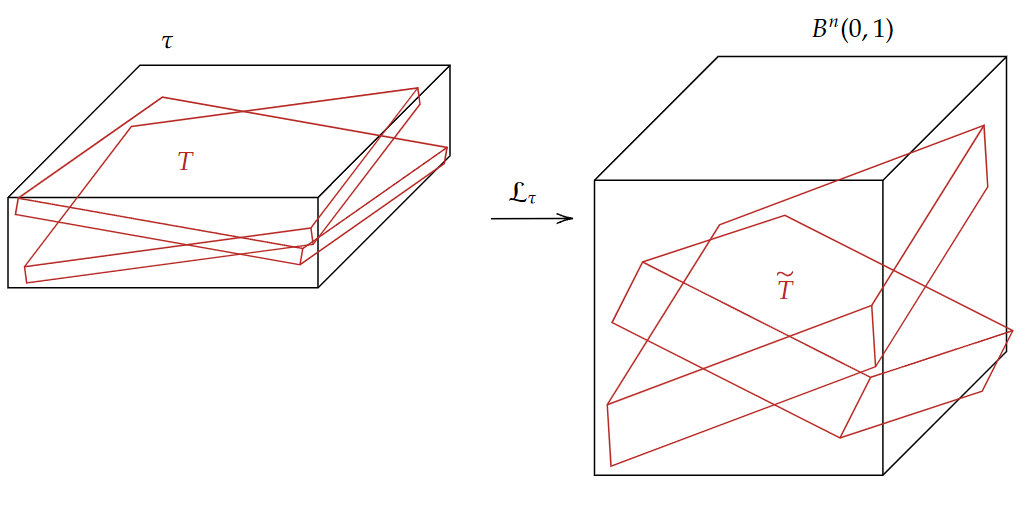
Figure 1. Rescaling

To estimate (64), we will first partition the integration domain. We partition $B^{n}(0,1)$ into slabs denoted by $\mathcal{T}=\{\tau\}$. Here each $\tau$ is a translation of $(V^{\circ})^{\perp}_{K^{-r+1}}$, and $\#\mathcal{T}\sim(K^{r-1})^{k}$. Since for each fixed $T\in\mathbb{T}_{V}$, there exists a $\tau\in\mathcal{T}$ such that $T\subset C\tau$ for some constant $C$. Therefore,

(65) $$\#\{\tau\in\mathcal{T}:T\cap\tau\neq\emptyset\}\lesssim 1.$$

We have

(66) $$\int_{B^{n}(0,1)}\prod_{i=1}^{d}(\sum_{V\in E\cap U_{i}}\sum_{T\in\mathbb{T}_{V}}1_{T})^{\frac{p}{d}}=\sum_{\tau}\int_{\tau}\prod_{i=1}^{d}(\sum_{V\in E\cap U_{i}}\sum_{T\in\mathbb{T}_{V},T\cap\tau\neq\emptyset}1_{T})^{\frac{p}{d}}.$$

Next, we will do the rescaling for each $\tau$. We first translate $\tau$ to the origin and do $K^{r-1}$-dilation in the orthogonal directions of $\tau$, so that $\tau$ roughly becomes $B^{n}(0,1)$. We denote this rescaling map by $\mathcal{L}_{\tau}=\mathcal{L}\circ T_{\tau}$, where $T_{\tau}$ is the translation and $\mathcal{L}$ is the dilation. After the rescaling, we see that each $T$ such that $T\cap\tau\neq\emptyset$ becomes a $\delta K^{r-1}\times\dots\times\delta K^{r-1}\times 1\times\dots\times 1$-slab contained in $B^{n}(0,1)$. We define them to be $\widetilde{T}$. See Figure 1. Taking into consideration of the rescaling factor, we have

(67) $$\int_{\tau}\prod_{i=1}^{d}(\sum_{V\in E\cap U_{i}}\sum_{T\in\mathbb{T}_{V},T\cap\tau\neq\emptyset}1_{T})^{\frac{p}{d}}=K^{-(r-1)(n-k)}\int_{B^{n}(0,1)}\prod_{i=1}^{d}(\sum_{V\in E\cap U_{i}}\sum_{T\in\mathbb{T}_{V},T\cap\tau\neq\emptyset}1_{\widetilde{T}})^{\frac{p}{d}}.$$

We want to rewrite the right hand side. Note that if $T\in\mathbb{T}_{V}$, then the core of $T$ is orthogonal to $V$, and hence parallel to $V^{\perp}$. Therefore, after the rescaling, the core of $\widetilde{T}$ is parallel to $\mathcal{L}(V^{\perp})$, and hence orthogonal to $(\mathcal{L}(V^{\perp}))^{\perp}$. This motivates us to define the following map

$$\begin{split}\mathcal{L}^{*}:G(k,n)\rightarrow G(k,n)\\ \mathcal{L}^{*}(V)=(\mathcal{L}(V^{\perp}))^{\perp}.\end{split}$$

We see that if $T\in\mathbb{T}_{V}$, then the core of $\widetilde{T}$ is orthogonal to $\mathcal{L}^{*}(V)$.

Next, we note that under the map $\mathcal{L}^{*}$, the $K^{-r}$-ball $U_{i}$ in $G(k,n)$ becomes an $O(K^{-1})$-ball which we denote by

$$\widetilde{U}_{i}:=\mathcal{L}^{*}(U_{i})=\{\mathcal{L}^{*}(V):V\in U_{i}\}.$$

Actually, one can verify that if $U_{i}=Q_{K^{-r}}(V_{i})$, then $\widetilde{U}_{i}$ is morally an $O(K^{-1})$-ball centered at $\mathcal{L}^{*}(V_{i})$. We briefly explain the reason: Since taking orthogonal complement gives an identification between $G(k,n)$ and $G(n-k,n)$, we can view $\{V^{\perp}:V\in U_{i}\}$ as a $K^{-r}$-ball in $G(n-k,n)$ centered at $V_{i}^{\perp}$; Then by Lemma 10, we see that $\{\mathcal{L}(V^{\perp}):V\in U_{i}\}$ is morally an $O(K^{-1})$-ball centered at $\mathcal{L}(V_{i}^{\perp})$; Finally by taking the orthogonal complement back, we see that $\widetilde{U}_{i}=\{(\mathcal{L}(V^{\perp}))^{\perp}:V\in U_{i}\}$ is morally an $O(K^{-1})$-ball centered at $\mathcal{L}^{*}(V_{i})$.

For $\widetilde{V}\in\widetilde{U}_{i}$, there is a $V\in U_{i}$ such that $\mathcal{L}^{*}(V)=\widetilde{V}$. Define

(68) $$\widetilde{\mathbb{T}}_{\widetilde{V},\tau}:=\{\widetilde{T}:T\in\mathbb{T}_{V},T\cap\tau\neq\emptyset\}.$$

By (65), we have

(69) $$\sum_{\tau}\#\widetilde{\mathbb{T}}_{\widetilde{V},\tau}\lesssim\#\mathbb{T}_{V}.$$

Now we can rewrite (67) as

(70) $$\int_{\tau}\prod_{i=1}^{d}(\sum_{V\in E\cap U_{i}}\sum_{T\in\mathbb{T}_{V},T\cap\tau\neq\emptyset}1_{T})^{\frac{p}{d}}=K^{-(r-1)(n-k)}\int_{B^{n}(0,1)}\prod_{i=1}^{d}(\sum_{\widetilde{V}\in\mathcal{L}^{*}(E\cap U_{i})}\sum_{\widetilde{T}\in\widetilde{\mathbb{T}}_{\widetilde{V},\tau}}1_{\widetilde{T}})^{\frac{p}{d}}.$$

The reason we do the rescaling is to use Brascamp-Lieb inequality at scale $K^{-1}$, as can be seen on the right hand side of (70) that $\mathcal{L}^{*}(E\cap U_{i})$ is contained in a $O(K^{-1})$-ball in $G(k,n)$. We will talk about it in the next subsection.

5.2. Brascamp-Lieb inequality

The version of Brascamp-Lieb inequality we are going to use is due to Maldague. See Theorem 2 in [10].

Theorem 25 (Maldague).

Let $W_{j}\in G(k,n)$ for $j=1,\dots,J$. Fix $p\in[1,J]$. Define

(71) $$\textup{BL}(\{W_{j}\}_{j=1}^{J},p):=\sup_{L\leq\mathbb{R}^{n}}(\dim L-\frac{p}{J}\sum_{j=1}^{J}\dim\pi_{W_{j}}(L)).$$

Here, $L\leq\mathbb{R}^{n}$ means $L$ is a subspace of $\mathbb{R}^{n}$, and $\pi_{W_{j}}:\mathbb{R}^{n}\rightarrow W_{j}$ is the orthogonal projection.

There exists $\nu>0$ depending on $\{W_{j}\}_{j=1}^{J}$, so that the following is true. For any $\varepsilon>0$ and for any $\mathcal{V}_{j}=\{V_{j}\}\subset A(n-k,n)\ (j=1,\dots,J)$ being sets of $(n-k)$-planes, such that each $V_{j}\in\mathcal{V}_{j}$ is orthogonal to some $W\in Q_{\nu}(W_{j})\subset G(k,n)$, we have

(72) $$\int_{[-1,1]^{n}}\prod_{j=1}^{J}\bigg{(}\sum_{V_{j}\in\mathcal{V}_{j}}1_{V_{j,\delta}}\bigg{)}^{\frac{p}{J}}\lesssim\delta^{n-\varepsilon}\delta^{-\textup{BL}(\{W_{j}\}_{j=1}^{J},p)}\prod_{j=1}^{J}\bigg{(}\#\mathcal{V}_{j}\bigg{)}^{\frac{p}{J}}.$$

By a compactness argument, we deduce the following result.

Theorem 26.

Let $\mathcal{W}_{j}\subset G(k,n)$ be a compact set for $j=1,\dots,J$. Fix $p\in[1,\infty)$. Define

(73) $$\textup{BL}(\{\mathcal{W}_{j}\}_{j=1}^{J},p):=\sup_{W_{1}\in\mathcal{W}_{1},\dots,W_{J}\in\mathcal{W}_{J}}\textup{BL}(\{W_{j}\}_{j=1}^{J},p).$$

Fix any $\varepsilon>0$. Then for any $\mathcal{V}_{j}=\{V_{j}\}\subset A(n-k,n)\ (j=1,\dots,J)$ being sets of $(n-k)$-planes, such that each $V_{j}\in\mathcal{V}_{j}$ is orthogonal to some $W\in\mathcal{W}_{j}$, we have

(74) $$\int_{[-1,1]^{n}}\prod_{j=1}^{J}\bigg{(}\sum_{V_{j}\in\mathcal{V}_{j}}1_{V_{j,\delta}}\bigg{)}^{\frac{p}{J}}\leq C(\{\mathcal{W}_{j}\},p,\varepsilon)\cdot\delta^{n-\varepsilon}\delta^{-\textup{BL}((\mathcal{W}_{j})_{j=1}^{J},p)}\prod_{j=1}^{J}\bigg{(}\#\mathcal{V}_{j}\bigg{)}^{\frac{p}{J}}.$$

We briefly explain how to use compactness argument to deduce Theorem 26 from Theorem 25. For any $\vec{W}=(W_{1},\dots,W_{J})\in\mathcal{W}_{1}\times\dots\times\mathcal{W}_{J}$, we use Theorem 25 to find a small number $\nu$, so that (74) is true when all the slabs are in $\nu$-neighborhood of $W_{j}^{\perp}$. In other words, there exists a $O(\nu)$-neighborhood of $(W_{1},\dots,W_{J})$, for which we call $B(\vec{W})$, so that (74) is true when all the slabs are in $B(\vec{W})$. Then we use the compactness of $\mathcal{W}_{1}\times\dots\times\mathcal{W}_{J}$ to find a finite covering using $B(\vec{W})$. Using this finite covering and splitting the LHS of (74) by triangle inequality, the proof of (74) is not hard.

We continue the estimate of (67). We recall (70) here:

(75) $$\int_{\tau}\prod_{i=1}^{d}(\sum_{V\in E\cap U_{i}}\sum_{T\in\mathbb{T}_{V},T\cap\tau\neq\emptyset}1_{T})^{\frac{p}{d}}=K^{-(r-1)(n-k)}\int_{B^{n}(0,1)}\prod_{i=1}^{d}(\sum_{\widetilde{V}\in\mathcal{L}^{*}(E\cap U_{i})}\sum_{\widetilde{T}\in\widetilde{\mathbb{T}}_{\widetilde{V},\tau}}1_{\widetilde{T}})^{\frac{p}{d}}.$$

Note that for each $i$, $\mathcal{L}^{*}(E\cap U_{i})\subset\mathcal{L}^{*}(U_{i})=\widetilde{U}_{i}$ is an $O(K^{-1})$-ball. Applying Theorem 26 with $J=d$, $\mathcal{W}_{i}=\widetilde{U}_{i}$, $\{V_{i,\delta}\}=\bigcup_{\widetilde{V}\in\mathcal{L}^{*}(E\cap U_{i})}\mathbb{T}_{\widetilde{V},\tau}$, we obtain

(76) $$\begin{split}\int_{B^{n}(0,1)}\prod_{i=1}^{d}(\sum_{\widetilde{V}\in\mathcal{L}^{*}(E\cap U_{i})}\sum_{\widetilde{T}\in\widetilde{\mathbb{T}}_{\widetilde{V},\tau}}1_{\widetilde{T}})^{\frac{p}{d}}&\leq C_{K}\delta^{n-\varepsilon^{2}}\delta^{-\textup{BL}}\prod_{j=1}^{d}(\sum_{\widetilde{V}\in\mathcal{L}^{*}(E\cap U_{i})}\#\widetilde{\mathbb{T}}_{\widetilde{V},\tau})^{\frac{p}{d}}\\ &\leq C_{K}\delta^{n-\varepsilon^{2}}\delta^{-\textup{BL}}(\sum_{\widetilde{V}\in\mathcal{L}^{*}(E)}\#\widetilde{\mathbb{T}}_{\widetilde{V},\tau})^{p}\end{split}$$

Here,

(77) $$\textup{BL}=\sup_{V_{1}\in\widetilde{U}_{1},\dots,V_{d}\in\widetilde{U}_{d}}\sup_{L\leq\mathbb{R}^{n}}(\dim L-\frac{p}{d}\sum_{j=1}^{d}\dim\pi_{V_{j}}(L)).$$

Combining (66), (67), (70), (76), and noting that we just bound the non-important factor $K^{-(r-1)(n-k)}$ in (70) by $1$, we obtain

(78) $$\begin{split}\int_{B^{n}(0,1)}\prod_{i=1}^{d}(\sum_{V\in E\cap U_{i}}\sum_{T\in\mathbb{T}_{V}}1_{T})^{\frac{p}{d}}&\leq C_{K}\delta^{n-\varepsilon^{2}}\delta^{-\textup{BL}}\sum_{\tau}(\sum_{\widetilde{V}\in\mathcal{L}^{*}(E)}\#\widetilde{\mathbb{T}}_{\widetilde{V},\tau})^{p}\\ &\leq C_{K}\delta^{n-\varepsilon^{2}}\delta^{-\textup{BL}}(\sum_{\tau}\sum_{\widetilde{V}\in\mathcal{L}^{*}(E)}\#\widetilde{\mathbb{T}}_{\widetilde{V},\tau})^{p}\\ (\textup{by~{}}\eqref{sumTV})&\lesssim C_{K}\delta^{n-\varepsilon^{2}}\delta^{-\textup{BL}}(\sum_{V\in E}\#\mathbb{T}_{V})^{p}\end{split}$$

Next, we consider the quantity BL. Fix $L\in G(l,n)$. Recalling the definition of $m(t,l)$ in Definition 4, we have

(79) $$E(m(t,l)-1,l)\leq t.$$

Noting that $E(m,l)$ is given by (7). For $L\in G(l,n)$, we have

(80) $$\dim(\{V\in G(k,n):\dim(\pi_{L}(V))\leq m(t,l)-1\})=E(m(t,l)-1,l)\leq t.$$

This means that

(81) $$\mathcal{M}_{L}:=\{V\in G(k,n):\dim(\pi_{L}(V))\leq m(t,l)-1\}$$

is at most a $t$-dimensional submanifold of $G(k,n)$. We also remark that for different $L\in G(l,n)$, the submanifolds (81) are isometric by symmetry. Noting that $\widetilde{U}_{i}$ ($1\leq i\leq d$) are disjoint $K^{-1}$-balls in $G(k,n)$, we have

(82) $$\#\{\widetilde{U}_{i}:1\leq i\leq d,\widetilde{U}_{i}\cap\mathcal{M}_{L}\neq\emptyset\}\lesssim K^{t}\leq K^{\tau-2\varepsilon}.$$

The last inequality is from (28). Returning to (77), we see that for any $V_{i}\in\widetilde{U}_{i}$ $(1\leq i\leq d)$ and $L\in G(l,n)$, there are more than $d-CK^{\tau-2\varepsilon}$ many $\widetilde{U}_{i}$ such that $\dim(\pi_{L}(V_{i}))\geq m(t,l)$, where $C$ is a constant. Also recall that $d=\lfloor K^{\tau-\varepsilon}\rfloor$. As a result, we have

(83) $$\begin{split}\textup{BL}&\leq\sup_{l\in\mathbb{Z}\cap[0,n]}(l-\frac{p}{d}(d-CK^{\tau-2\varepsilon})m(t,l))\\ &\leq\sup_{l\in\mathbb{Z}\cap[0,n]}(l-p(1-2CK^{-\varepsilon})m(t,l))\\ &\leq\sup_{l\in\mathbb{Z}\cap[0,n]}(l-p\cdot m(t,l))+\varepsilon\\ &=\lambda_{p}+\varepsilon,\end{split}$$

if $K$ is large enough.

Combining (63) and (78), and noting that there are $\lesssim\delta^{-\varepsilon}$ terms on the RHS of (63), we obtain

(84) $$\int_{W}\Big{(}\sum_{V\in E}\sum_{T\in\mathbb{T}_{V}}1_{T}\Big{)}^{p}\lesssim_{\varepsilon,p}\delta^{-O(\varepsilon)}\delta^{n}\delta^{-\lambda_{p}}(\delta^{-\sigma-\tau})^{p}.$$

Renaming $O(\varepsilon)$ to be $\gamma$ will give (24).

6. Lower bounds for $T(a,s)$

In this section, we prove some lower bounds for $T(a,s)$ (see (1)). For each pair $(a,s)$, we will construct an example $A\subset\mathbb{R}^{n}$ and calculate the dimension of the exceptional set

$$\dim(\{V\in G(k,n):\dim(\pi_{V}(A))<s\}).$$

We remark that in the setting of finite field, examples were built for some specific pairs $(a,s)$ in [2].

We first recall the theorem of Ren and Wang [17]:

Theorem 27.

Let $A\subset\mathbb{R}^{2}$ with $\dim(A)=a$. For $\theta\in G(1,\mathbb{R}^{2})$, let $\pi_{\theta}:\mathbb{R}^{2}\rightarrow\theta$ be the orthogonal projection onto line $\theta$. For $0<s<\max\{1,a\}$, define $E_{s}(A):=\{\theta:\dim(\pi_{\theta}(A))<s\}$. Then

(85) $$\dim(E_{s}(A))\leq\max\{0,2s-a\}.$$

For our purpose, we are interested in the sharp example $A\subset\mathbb{R}^{2}$ for which (85) holds with “$\leq$” replaced by “$=$”. Actually, there exists $\boldsymbol{A}_{s,a}\subset\mathbb{R}^{2}$ with $\dim(\boldsymbol{A}_{s,a})=a$ such that $\boldsymbol{E}_{s,a}:=E_{s}(\boldsymbol{A}_{s,a})$ has Hausdorff dimension $\geq 2s-a$. For this example, see Section 5.4 in [13]. We would like to formally state it as a proposition.

Proposition 28.

For $0<a<2$, $\frac{a}{2}\leq s<\min\{1,a\}$. There exists a set $\boldsymbol{A}_{s,a}\subset\mathbb{R}^{2}$ with $\dim(\boldsymbol{A}_{s,a})=a$ such that

(86) $$\boldsymbol{E}_{s,a}:=\{\theta\in G(1,2):\dim(\pi_{\theta}(\boldsymbol{A}_{s,a}))<s\}$$

has Hausdorff dimension $2s-a$.

The sets $\boldsymbol{A}_{s,a}$ and $\boldsymbol{E}_{s,a}$ will serve as building blocks when we construct examples for all $n$. We would like to spend some time explaining a construction of $\boldsymbol{A}_{s,a}$ and $\boldsymbol{E}_{s,a}$ in the finite setting. It is exactly the sharp example of the Szemerédi-Trotter theorem.

Example 29.

Let $N$ be a large number. We assume $2s\geq a$. Consider a set of lines $\mathcal{L}=\{l_{k,m}:|k|\leq N^{2s-a},|m|\leq 10N^{s}\}$ in $\mathbb{R}^{2}$. Here, $k$ and $m$ are integers and $l_{k,m}$ is given by

$$l_{k.m}:y=kx+m.$$

We see that $\mathcal{L}$ consists of lines from $\sim N^{2s-a}$ many directions, and in each of these directions there are $\sim N^{s}$ many lines. We denote these directions by $E$, and for $\theta\in E$, let $\mathcal{L}_{\theta}$ be the lines in $\mathcal{L}$ that are in direction $\theta$.

Consider the set $A:=\{(x,y)\in\mathbb{Z}^{2}:|x|\leq N^{a-s},|y|\leq N^{s}\}$. For any $|k|\leq N^{2s-a}$, we see that any $(x,y)\in A$ satisfies $|y-kx|\leq 10N^{s}$. This means that for any direction $\theta\in E$, $A$ is covered by $\mathcal{L}_{\theta}$. Therefore we have for each $\theta\in E$,

$$\#\pi_{\theta}(A)\leq\#\mathcal{L}_{\theta}\lesssim N^{s}.$$

We obtain the following estimate:

$$\#\{\theta:\#\pi_{\theta}(A)\lesssim N^{s}\}\geq\#E\sim N^{2s-a}.$$

Such $A$ and $E$ are like the discrete analogue of $\boldsymbol{A}_{s,a}$ and $\boldsymbol{E}_{s,a}$.

6.1. Examples in $\mathbb{R}^{3}$

To give more insight, we first focus on the projection to lines and planes in $\mathbb{R}^{3}$. In other words, we consider the case $n=3$, $k=1$ or $2$.

Example 30 (Projections to lines in $\mathbb{R}^{3}$).

1. When $a\leq 1$, let $A$ be contained in the $x_{3}$-axis. We see that for any line $\ell$ that is parallel to the $(x_{1},x_{2})$-plane, the projection of $A$ onto $\ell$ has dimension $0(<s)$. Therefore $\dim(E_{s}(A))\geq 1$.

2. Consider the case $1<a\leq 2$.

   $\bullet$ When $\frac{a-1}{2}<s<a-1$, we choose $A=\boldsymbol{A}_{s,a-1}\times\mathbb{R}$. This looks like the left picture in Figure 2. We only look at those directions $\theta$ that are parallel to the $(x_{1},x_{2})$-plane. This is just the problem in $\mathbb{R}^{2}$. We see that $E_{s}(A)\supset\mathbf{E}_{s,a-1}$, so

   $$\dim(E_{s}(A))\geq\max\{0,2s-(a-1)\}=\max\{0,1+2s-a\}.$$

   $\bullet$ When $a-1<s<1$, we choose $A=A^{\prime}\times\mathbb{R}$, where $A^{\prime}\subset\mathbb{R}^{2}$ is any set with $\dim(A^{\prime})=a-1$. We see that if $\theta$ is parallel to the $(x_{1},x_{2})$-plane, then $\pi_{\theta}(A)=\pi_{\theta}(A^{\prime})$ has dimension less than $\dim(A^{\prime})=a-1<s$. Therefore,

   $$\dim(E_{s}(A))\geq 1.$$

3. Consider the case $2<a\leq 3$. When $\frac{a-1}{2}<s<1$, we choose $A=\boldsymbol{A}_{s,a-1}\times\mathbb{R}$ (then $\dim(A)=\dim(\boldsymbol{A}_{s,a-1})+\dim(\mathbb{R})=a$). We only look at those directions $\theta$ that are parallel to the $(x_{1},x_{2})$-plane. This is just the problem in $\mathbb{R}^{2}$. We see that $E_{s}(A)\supset\boldsymbol{E}_{s,a-1}$, so

   $$\dim(E_{s}(A))\geq\max\{0,2s-(a-1)\}=\max\{0,1+2s-a\}.$$

Figure 2. Projection to planes

Example 31 (Projections to planes in $\mathbb{R}^{3}$).

1. When $a\leq 1$, let $A=\boldsymbol{A}_{s,a}\times\{0\}$. For $\theta\in S^{2}$, we use $V_{\theta}$ to denote the plane orthogonal to $\theta$. We only look at the projection of $A$ to those $V_{\theta}$ where $\theta$ is parallel to the $(x_{1},x_{2})$-plane. This exactly becomes a projection-to-line problem in $\mathbb{R}^{2}$, so we have that $\dim(E_{s}(A))\geq\dim(\boldsymbol{E}_{s,a})\geq\max\{0,2s-a\}$.

2. Consider the case $1<a\leq 2$.

   $\bullet$ When $s\leq 1$, we use the same example as in the last paragraph.

   $\bullet$ When $1<s\leq\frac{a+1}{2}$, we choose $A$ to be a subset of $\mathbb{R}^{2}\times\{0\}$. Then for those $\theta$ parallel to $(x_{1},x_{2})$-axis, the projection of $A$ onto $V_{\theta}$ is contained in the line $(\mathbb{R}^{2}\times\{0\})\cap V_{\theta}$ which has dimension $\leq 1<s$. This means that these $V_{\theta}$ are in the exceptional set. So, $\dim(E_{s}(A))\geq 1$.

   $\bullet$ When $\frac{a+1}{2}<s<a$, we choose $A=\boldsymbol{A}_{s-1,a-1}\times\mathbb{R}$ (see Figure 2). For a direction $\theta$ that is parallel to the $(x_{1},x_{2})$-plane, we use $\ell_{\theta}$ to denote the line contained in $\mathbb{R}^{2}\times\{0\}$ that is orthogonal to $\theta$, i.e., $\ell_{\theta}=V_{\theta}\cap(\mathbb{R}^{2}\times\{0\})$. Suppose $\ell_{\theta}$ is in $\boldsymbol{E}_{s-1,a-1}$, i.e., $\dim(\pi_{\ell_{\theta}}(\boldsymbol{A}_{s-1,a-1}))<s-1$. Then noting that $\pi_{V_{\theta}}(\boldsymbol{A}_{s-1,a-1}\times\mathbb{R})=\pi_{\ell_{\theta}}(\boldsymbol{A}_{s-1,a-1})\times\mathbb{R}$, we have $\dim(\pi_{V_{\theta}}(A))=\dim(\pi_{\ell_{\theta}}(\boldsymbol{A}_{s-1,a-1}))+1<s$. On the right hand side of Figure 2, we draw a bunch of planes that contain $\ell_{\theta}$ but not contain the $x_{3}$-axis. We can view these planes as

   (87) $$\mathbb{R}\mathbb{P}^{1}\setminus\{*\},$$

   where $*$ corresponds to the $(x_{1},x_{2})$-plane. The geometric observation is that the projection of $A$ onto these planes are the same, and hence has dimension $<s$. We see that

   $$\dim(E_{s}(A)) \geq\dim(\boldsymbol{E}_{s-1,a-1}\times(\mathbb{R}\mathbb{P}^{1}\setminus\{*\}))$$

   $$=\dim(\boldsymbol{E}_{s-1,a-1})+\dim(\mathbb{R}\mathbb{P}^{1}\setminus\{*\})$$

   $$\geq 2(s-1)-(a-1)+1=2s-a.$$

   We used that $\dim(\boldsymbol{E}_{s-1,a-1})\geq\max\{0,2(s-1)-(a-1)\}=2(s-1)-(a-1)$ since $\frac{a+1}{2}<s$.

3. Consider the case $2<a\leq 3$.

   $\bullet$ When $a-1<s<\frac{a+1}{2}$, we choose $A$ to be contained in $\mathbb{R}^{2}\times I$, where $I\subset\mathbb{R}$ has dimension $a-2$. Then for those $\theta$ parallel to $(x_{1},x_{2})$-axis, the projection of $A$ onto $V_{\theta}$ is contained in $\ell_{\theta}\times I$ which has dimension $\leq 1+a-2=a-1<s$. This means that these $V_{\theta}$ are in the exceptional set. So, $\dim(E_{s}(A))\geq 1$.

   $\bullet$ When $\frac{a+1}{2}<s<2$, we just use the same example $A=\boldsymbol{A}_{s-1,a-1}\times\mathbb{R}$ as above to get the lower bound $\dim(E_{s}(A))\geq 2s-a$.

We summarize our examples as follows.

Proposition 32 (Projections to lines in $\mathbb{R}^{3}$).

Consider the projection to lines in $\mathbb{R}^{3}$, so $E_{s}(A)$ is given by (2) with $k=1,n=3$. We have

1. When $a\leq 1:$ $T(a,s)\geq 1$;

2. When $1<a\leq 2:$

   $$T(a,s)\geq\begin{cases}0&s\leq\frac{a-1}{2}\\ 1+2s-a&\frac{a-1}{2}<s\leq a-1\\ 1&a-1<s<1\end{cases}$$

3. When $2<a\leq 3:$

   $$T(a,s)\geq\begin{cases}0&s\leq\frac{a-1}{2}\\ 1+2s-a&\frac{a-1}{2}<s<1\end{cases}$$

Proposition 33 (Projections to planes in $\mathbb{R}^{3}$).

Consider the projection to planes in $\mathbb{R}^{3}$, so $E_{s}(A)$ is given by (2) with $k=2,n=3$. We have

1. When $a\leq 1:$ $T(a,s)\geq\max\{0,2s-a\}$;

2. When $1<a\leq 2:$

   $$T(a,s)\geq\begin{cases}0&s\leq\frac{a}{2}\\ 2s-a&\frac{a}{2}<s\leq 1\\ 1&1<s\leq\frac{a+1}{2}\\ 2s-a&\frac{a+1}{2}<s<a\end{cases}$$

3. When $2<a\leq 3:$

   $$T(a,s)\geq\begin{cases}0&s\leq a-1\\ 1&a-1<s\leq\frac{a+1}{2}\\ 2s-a&\frac{a+1}{2}<s<2\end{cases}$$

Remark 34.

To construct analogous examples in higher dimensions, we can play the same trick. For example, choose $A=\boldsymbol{A}_{s^{\prime},a^{\prime}}\times\mathbb{R}^{l}$, or $I\times\mathbb{R}^{l^{\prime}}$. Then we may find the lower bound of $T(a,s)$ are of forms $m+2s-a$, or $m^{\prime}$, for some integers $m,m^{\prime}$. We will talk about the examples in higher dimensions in the next subsection.

6.2. Examples in higher dimensions

We discuss the examples of the exceptional sets in higher dimensions. There will be four types of the examples. We will use $d(m,n)$ to denote $\dim(G(m,n))$, namely $d(m,n)=m(n-m)$. We first list some well known facts.

Lemma 35.

Suppose $V,W\subset\mathbb{R}^{n}$ are two subspaces. Then

$$\dim(\pi_{V}(W))=\dim(\pi_{W}(V)),$$

and

$$\dim(\pi_{V}(W))=\dim(W)-\dim(W\cap V^{\perp}).$$

Proof.

Since the linear map $\pi_{V}:W\rightarrow V$ has kernel $W\cap V^{\perp}$, we have

$$\dim(\pi_{V}(W))=\dim(W)-\dim(W\cap V^{\perp}).$$

To prove the first equality, we note

$$\dim(\pi_{V}(W)) =\dim(W)-\dim(W\cap V^{\perp})$$

$$=\dim W-\bigg{(}n-\dim\big{(}(W\cap V^{\perp})^{\perp}\big{)}\bigg{)}$$

$$=\dim W-n+\dim(W^{\perp}+V)$$

$$=\dim W-n+\dim W^{\perp}+\dim V-\dim(W^{\perp}\cap V)$$

$$=\dim V-\dim(V\cap W^{\perp})$$

$$=\dim(\pi_{W}(V)).$$

∎

Lemma 36.

Let $0\leq l\leq n$, $1\leq k,m\leq n$ be integers satisfying $n-k\geq m-l$ and $l\leq k,m$. If $W\in G(m,n)$, then

$$\dim\{V\in G(k,n):\dim(\pi_{V}(W))\leq l\}=d(k-l,n-m)+d(l,n-(k-l)).$$

Proof.

By Lemma 35, we have

$$\{V\in G(k,n):\dim(\pi_{V}(W))\leq l\} =\{V\in G(k,n):\dim(V\cap W^{\perp})\geq k-l\},$$

By condition $l\leq k$, we see $\dim(V\cap W^{\perp})\geq k-l$ makes sense. Actually, $\{V\in G(k,n):\dim(V\cap W^{\perp})\geq k-l\}$ is a Schubert cycle whose dimension is not hard to calculate (see [7] Chapter 1, Section 5). Here, we provide a sketch of proof. The condition $n-k\geq m-l$ says that $\dim(W^{\perp})\geq k-l$. The condition $l\leq m$ yields that generic $V\in G(k,n)$ satisfies $\dim(V\cap W^{\perp})=\dim(V)+\dim(W^{\perp})-n=k+n-m-n\leq k-l$ (imagine the generic case is when $V$ and $W^{\perp}$ are as transverse as possible). Therefore, generic $V\in\{V\in G(k,n):\dim(V\cap W^{\perp})\geq k-l\}$ will satisfy $\dim(V\cap W^{\perp})=k-l$. It is equivalent to calculate the dimension of

$$\{V\in G(k,n):\dim(V\cap W^{\perp})=k-l\}.$$

Note that we can identify $V$ with $(v_{1},\dots,v_{k})$, where $\{v_{i}\}_{i=1}^{k}$ are orthonormal basis of $V$. We first choose $v_{1},\dots,v_{k-l}\in W^{\perp}$, which is equivalent to choosing an $(k-l)$-plane in $W^{\perp}$. It gives $d(k-l,n-m)$-dimensional choices. Next, we choose $v_{k-l+1},\dots,v_{k}$ from $\textup{span}\{v_{1},\dots,v_{k-l}\}^{\perp}$, which gives $d(l,n-(k-l))$-dimensional choices. Adding together, gives the dimension $d(k-l,n-m)+d(l,n-(k-l))$. ∎

We state the key result.

Proposition 37.

Fix $0<k<n$. For $A\subset\mathbb{R}^{n}$, define

$$E_{s}(A):=\{V\in G(k,n):\dim(\pi_{V}(A))<s\}.$$

For $0<a<n$ and $0<s\leq\min\{k,a\}$, define

$$T(a,s):=\sup_{\dim(A)=a}\dim(E_{s}(A)).$$

Then we have the following lower bound for $T(a,s)$. We write $a=m+\beta,s=l+\gamma$ where $m,l\in\mathbb{N}$ and $\beta,\gamma\in(0,1]$.

1. Type 1: $1\leq m\leq n+l-k,\gamma>\frac{\beta+1}{2}$

   (88) $$T(m+\beta,l+\gamma) \geq d(k-l,n-m)+d(l,n-(k-l))+2\gamma-(\beta+1)$$

   $$=k(n-k)-(m-l)(k-l)+2\gamma-(\beta+1).$$

2. Type 2: $m\leq n+l-k,\gamma>\beta$

   (89) $$T(m+\beta,l+\gamma) \geq d(k-l,n-m)+d(l,n-(k-l))$$

   $$=k(n-k)-(m-l)(k-l).$$

3. Type 3: $m\leq n+l-k-1,\gamma>\frac{\beta}{2}$

   (90) $$T(m+\beta,l+\gamma) \geq d(k-l,n-m-1)+d(l,n-(k-l))+2\gamma-\beta$$

   $$=k(n-k)-(m+1-l)(k-l)+2\gamma-\beta.$$

4. Type 4: $1\leq l,m\leq n+l-k-1$

   (91) $$T(m+\beta,l+\gamma) \geq d(k-(l-1),n-m)+d(l-1,n-(k-l+1))$$

   $$=k(n-k)-(m-l+1)(k-l+1).$$

Proof.

Type 2: When $n-m\geq k-l,\gamma>\beta$, then

(92) $$T(m+\beta,l+\gamma)\geq d(k-l,n-m)+d(l,n-(k-l))=k(n-k)-(m-l)(k-l).$$

We choose $A=\mathbb{R}^{m}\times I\times\{\underbrace{(0,\dots,0)}_{(n-m-1)\times 0}\}$, where $I\subset\mathbb{R}$ has Hausdorff dimension $\beta$. For simplicity, we just write $A=\mathbb{R}^{m}\times I$. We want to find those $V\in G(k,n)$ such that $\dim(\pi_{V}(A))<l+\gamma$. We note that if $V$ satisfies $\dim(\pi_{V}(\mathbb{R}^{m}))\leq l$, then $\dim(\pi_{V}(\mathbb{R}^{m}\times I))\leq l+\beta<l+\gamma$, which means $V\in E_{s}(A)$. This shows that

$$E_{s}(A)\supset\{V\in G(k,n):\dim(\pi_{V}(\mathbb{R}^{m}))\leq l\}.$$

By Lemma 36, the right hand side has dimension $d(k-l,n-m)+d(l,n-(k-l))$. This gives (92).

Type 3: When $n-m-1\geq k-l,\gamma>\frac{\beta}{2}$, then

(93) $$T(m+\beta,l+\gamma) \geq d(k-l,n-m-1)+d(l,n-(k-l))+2\gamma-\beta$$

$$=k(n-k)-(m+1-l)(k-l)+2\gamma-\beta.$$

We choose $A=\boldsymbol{A}_{\gamma,\beta}\times\mathbb{R}^{m}\times\{\underbrace{(0,\dots,0)}_{(n-m-2)\times 0}\}$. Recall that $\boldsymbol{A}_{\gamma,\beta}\subset\mathbb{R}^{2}$ is the example discussed in Proposition 28. We will use $\mathbb{R}^{2}$ to denote $\mathbb{R}^{2}\times\{\underbrace{(0,\dots,0)}_{(n-2)\times 0}\}$. We use $\mathbb{R}^{m}$ to denote $\{(0,0)\}\times\mathbb{R}^{m}\times\{(0,\dots,0)\}$. For each direction $\theta$ parallel to $\mathbb{R}^{2}$, we use $\ell_{\theta}$ to denote the line parallel to $\mathbb{R}^{2}$ but orthogonal to $\theta$. We define

$$\mathcal{U}_{\theta}=\{V\in G(k,n):\dim(\pi_{V}(\mathbb{R}\theta\oplus\mathbb{R}^{m}))\leq l,\dim(\pi_{V}(\mathbb{R}^{m}))=l,\dim(\pi_{V}(\mathbb{R}^{2}\times\mathbb{R}^{m}))=l+1\},$$

$$\mathcal{V}_{\theta}=\{V\in G(k,n):\dim(\pi_{V}(\mathbb{R}\theta\oplus\mathbb{R}^{m}))\leq l\},$$

$$\mathcal{W}_{\theta}=\{V\in\mathcal{V}_{\theta}:\dim(\pi_{V}(\mathbb{R}^{m}))\leq l-1\}\cup\{V\in\mathcal{V}_{\theta}:\dim(\pi_{V}(\mathbb{R}^{2}\times\mathbb{R}^{m})\leq l\}.$$

It is not hard to see $\mathcal{U}_{\theta}=\mathcal{V}_{\theta}\setminus\mathcal{W}_{\theta}$. To get some intuition on these sets, we suggest readers to look back at (87). $\mathcal{U}_{\theta},\mathcal{V}_{\theta}$ and $\mathcal{W}_{\theta}$ are higher dimensional analog of $\mathbb{R}\mathbb{P}^{1}\setminus\{*\},\mathbb{R}\mathbb{P}^{1}$ and $\{*\}$.

Let $\mathbf{E}_{\gamma,\beta}=\{\theta\in S^{1}:\dim(\pi_{l_{\theta}}(\boldsymbol{A}_{\gamma,\beta}))<\gamma\}$. We claim that if $\theta\in\mathbf{E}_{\gamma,\beta}$, then $\mathcal{V}_{\theta}\subset E_{l+\gamma}(A)$. In other words, any $V\in\mathcal{V}_{\theta}$ satisfies $\dim(\pi_{V}(A))<l+\gamma$. We first note that $\boldsymbol{A}_{\gamma,\beta}\subset\pi_{l_{\theta}}(\boldsymbol{A}_{\gamma,\beta})+\mathbb{R}\theta$, so

$$A=\boldsymbol{A}_{\gamma,\beta}\times\mathbb{R}^{m}\subset(\pi_{l_{\theta}}(\boldsymbol{A}_{\gamma,\beta})+\mathbb{R}\theta)\times\mathbb{R}^{m}=\pi_{l_{\theta}}(\boldsymbol{A}_{\gamma,\beta})+(\mathbb{R}\theta\oplus\mathbb{R}^{m}).$$

Therefore,

$$\dim(\pi_{V}(A))\leq\dim(\pi_{l_{\theta}}(\boldsymbol{A}_{\gamma,\beta}))+\dim(\pi_{V}(\mathbb{R}\theta\oplus\mathbb{R}^{m}))<\gamma+l.$$

We see that $E_{l+\gamma}(A)\supset\bigcup_{\theta\in\mathbf{E}_{\gamma,\beta}}\mathcal{V}_{\theta}.$ $\mathcal{V}_{\theta}$ may intersect with each other, so we delete a tiny portion $\mathcal{W}_{\theta}$ from $\mathcal{V}_{\theta}$, so that the remaining part $\mathcal{U}_{\theta}=\mathcal{V}_{\theta}\setminus\mathcal{W}_{\theta}$ are disjoint with each other. Then we have

$$E_{l+\gamma}(A)\supset\bigsqcup_{\theta\in\mathbf{E}_{\gamma,\beta}}\mathcal{U}_{\theta}.$$

To make the argument precise, we first apply Lemma 36 to see

$$\dim(\mathcal{V}_{\theta})=d(k-l,n-m-1)+d(l,n-(k-l))=k(n-k)-(m+1-l)(k-l).$$

To calculate $\dim(\mathcal{W}_{\theta})$, we apply Lemma 36 again to see

$$\dim(\{V\in G(k,n):\dim(\pi_{V}(\mathbb{R}^{m}))\leq l-1\})=k(n-k)-(m-l+1)(k-l+1),$$

and

$$\dim(\{V\in G(k,n):\dim(\pi_{V}(\mathbb{R}^{2}\times\mathbb{R}^{m}))\leq l\})=k(n-k)-(m+2-l)(k-l).$$

Therefore, $\dim(\mathcal{W}_{\theta})<\dim(\mathcal{V}_{\theta})$ and hence

$$\dim(\mathcal{U}_{\theta})=\dim(\mathcal{V}_{\theta})=d(k-l,n-m-1)+d(l,n-(k-l)).$$

Next we show $\mathcal{U}_{\theta}\cap\mathcal{U}_{\theta^{\prime}}=\emptyset$ for $\theta\neq\theta^{\prime}$. By contradiction, suppose $V\in\mathcal{U}_{\theta}\cap\mathcal{U}_{\theta^{\prime}}$. By definition, $V$ satisfies

$$\dim(\pi_{V}(\mathbb{R}\theta\oplus\mathbb{R}^{m}))\leq l,$$

$$\dim(\pi_{V}(\mathbb{R}\theta^{\prime}\oplus\mathbb{R}^{m}))\leq l,$$

$$\dim(\pi_{V}(\mathbb{R}^{m}))=l,$$

$$\dim(\pi_{V}(\mathbb{R}^{2}\times\mathbb{R}^{m}))=l+1.$$

The first and third conditions imply $\pi_{V}(\mathbb{R}\theta)\subset\pi_{V}(\mathbb{R}^{m})$. Similarly, the second and third conditions imply $\pi_{V}(\mathbb{R}\theta^{\prime})\subset\pi_{V}(\mathbb{R}^{m})$. Noting that $\textup{span}\{\mathbb{R}\theta,\mathbb{R}\theta^{\prime}\}=\mathbb{R}^{2}$, we have

$$\pi_{V}(\mathbb{R}^{2}\times\mathbb{R}^{m})\subset\pi_{V}(\mathbb{R}^{m}),$$

which has dimension $=l$, contradicting the fourth condition.

We have shown that $E_{l+\gamma}(A)\supset\bigsqcup_{\theta\in\mathbf{E}_{\gamma,\beta}}\mathcal{U}_{\theta}$, which has dimension $\dim(\mathbf{E}_{\gamma,\beta})+\dim(\mathcal{U}_{\theta})$

$$=2\gamma-\beta+d(k-l,n-m-1)+d(l,n-(k-l)).$$

This gives (93).

Type 1 : When $m\geq 1,n-m\geq k-l,\gamma>\frac{\beta+1}{2}$, then

(94) $$T(m+\beta,l+\gamma) \geq d(k-l,n-m)+d(l,n-(k-l))+2\gamma-(\beta+1)$$

(95) $$=k(n-k)-(m-l)(k-l)+2\gamma-(\beta+1).$$

The trick is to write $T(m+\beta,l+\gamma)=T((m-1)+(\beta+1),l+\gamma)$ and then apply Type 2 construction. We will choose

$$A=\boldsymbol{A}_{\gamma,\beta+1}\times\mathbb{R}^{m-1}\times\{(0,\dots,0)\}.$$

It will give the bound (94).

Type 4 : When $l\geq 1,n-m\geq k-l+1$, then

(96) $$T(m+\beta,l+\gamma) \geq d(k-(l-1),n-m)+d(l-1,n-(k-l+1))$$

$$=k(n-k)-(m-l+1)(k-l+1).$$

The idea is to apply Type 1 construction. Note that here we do not have the condition $\gamma>\beta$, so we cannot directly apply Type 1. The trick is to write

$$T(m+\beta,l+\gamma)\geq T(m+\beta,(l-1)+1).$$

Now our new $l$ becomes $l-1$, and our new $\gamma$ becomes $1$. We apply Type 1, and obtain (96). ∎

Given $a=m+\beta,s=l+\gamma$, we compare the lower bounds of these four types and see that

$${\bf Type\ 1}\geq{\bf Type\ 2}\geq{\bf Type\ 3}\geq{\bf Type\ 4}.$$

Therefore, the strategy to find the lower bound of $T(a,s)$ is by testing the requirement of Type 1, Type 2,… one by one, and use the lower bound as soon as the requirement is satisfied. If neither requirement is satisfied, then we only expect the trivial lower bound $T(a,s)\geq 0$.

For our application in Theorem 7, we only use Type 2 example.

6.3. Proof of Theorem 7

We will use Type 2 bound in Proposition 37. We consider the case $k\leq\frac{n}{2}$. Suppose $\beta\in(0,1],\gamma\in(\beta,\frac{k}{n}(1+\beta)]$. By Theorem 1, we have

(97) $$T(1+\beta,\gamma)\leq T(1+\beta,\frac{k}{n}(1+\beta))\leq k(n-k)-k.$$

To obtain a lower bound, we use Type 2. We choose $m=1,l=0$, so $a=1+\beta$ and $s=\gamma$. We can verify the condition that $m\leq n+l-k,\gamma>\beta$. Therefore, we obtain

(98) $$T(1+\beta,\gamma)\geq k(n-k)-k.$$

This finishes the proof that

(99) $$T(1+\beta,\gamma)=k(n-k)-k.$$

Next, we consider the case $k\geq\frac{n}{2}$. Suppose $\beta\in(0,1],\gamma\in(\beta,(1-\frac{k}{n})+\frac{k}{n}\beta]$. By Theorem 1, we have

(100) $$T(n-1+\beta,k-1+\gamma)\leq T(n-1+\beta,\frac{k}{n}(n-1+\beta))\leq k(n-k)-(n-k).$$

To obtain a lower bound, we use Type 2. We choose $m=n-1,l=k-1$, so $a=n-1+\beta$ and $s=k-1+\gamma$. We can verify the condition that $m\leq n+l-k,\gamma>\beta$. Therefore, we obtain

(101) $$T(n-1+\beta,k-1+\gamma)\geq k(n-k)-(n-k).$$

This finishes the proof that

(102) $$T(n-1+\beta,k-1+\gamma)=k(n-k)-(n-k).$$

References

- [1] J. Bourgain. The discretized sum-product and projection theorems. J. Anal. Math., 112(1):193–236, 2010.
- [2] P. Bright and S. Gan. Exceptional set estimates in finite fields. arXiv preprint arXiv:2302.13193, 2023.
- [3] K. Falconer. Hausdorff dimension and the exceptional set of projections. Mathematika, 29(1):109–115, 1982.
- [4] K. Fässler and T. Orponen. On restricted families of projections in . Proc. Lond. Math. Soc., 109(2):353–381, 2014.
- [5] S. Gan. Hausdorff dimension of unions of -planes. arXiv preprint arXiv:2305.14544, 2023.
- [6] S. Gan, S. Guo, L. Guth, T. L. Harris, D. Maldague, and H. Wang. On restricted projections to planes in . arXiv preprint, 2022.
- [7] P. Griffiths and J. Harris. Principles of algebraic geometry. John Wiley & Sons, 2014.
- [8] W. He. Orthogonal projections of discretized sets. J. Fractal Geom., 7(3):271–317, 2020.
- [9] R. Kaufman. On hausdorff dimension of projections. Mathematika, 15(2):153–155, 1968.
- [10] D. Maldague. Regularized Brascamp–Lieb inequalities and an application. Q. J. Math., 73(1):311–331, 2022.
- [11] J. M. Marstrand. Some fundamental geometrical properties of plane sets of fractional dimensions. Proc. Lond. Math. Soc., 3(1):257–302, 1954.
- [12] P. Mattila. Hausdorff dimension, orthogonal projections and intersections with planes. Ann. Acad. Sci. Fenn. Ser. AI Math, 1(2):227–244, 1975.
- [13] P. Mattila. Fourier analysis and Hausdorff dimension, volume 150. Cambridge University Press, 2015.
- [14] T. Orponen and P. Shmerkin. On the Hausdorff dimension of Furstenberg sets and orthogonal projections in the plane. arXiv preprint arXiv:2106.03338, 2021.
- [15] T. Orponen and P. Shmerkin. Projections, Furstenberg sets, and the ABC sum-product problem. arXiv preprint arXiv:2301.10199, 2023.
- [16] Y. Peres and W. Schlag. Smoothness of projections, Bernoulli convolutions, and the dimension of exceptions. Duke Math. J., 2000.
- [17] K. Ren and H. Wang. Furstenberg sets estimate in the plane. arXiv preprint arXiv:2308.08819, 2023.